Dynamics of a collection of active particles on a two-dimensional periodic undulated surface

Abstract

We study the dynamics of circular disk shaped active particles (AP) on a two dimensional periodic undulated surface. Each particle has an internal energy mechanism which is modeled by an active friction force and it is controlled by an activity parameter $v_{0}$. It acts as negative friction if the speed of the particle is smaller than $v_{0}$ and normal friction otherwise. Surface undulation is modeled by the periodic undulation of fixed amplitude and wavelength. The dynamics of the particle is studied for different activities and surface undulations (SU). Three types of particle dynamic is observed on varying activity and SU: confined, early time subdiffusion to diffusion and super diffusion to late time diffusion. An effective equilibirum is established by showing the Green-Kubo relation between the effective diffusivity and the velocity auto-correlation function for all activities and small SU.

I Introduction

In last few decades, active systems have become a subject of great interest sriramannulrev ; marchettirmp ; romanczuk ; bechinger due to their unusual properties in comparison to the system at thermal equilibrium. Examples start from systems of micron scale like, bacterial colonies dell up to a few meters like fish school fishschool , bird flock flock etc. and also artificial microparticles like Janus particles filly ; tailleur ; cates2015 ; cates2013 . Each constituent in these systems takes energy from their surroundings, and convert the energy into persistent motion which leads to nonequilibrium behaviour. Interestingly, the collective behaviour and phase separation is observed, even in the absence of any external drive sriramannulrev ; marchettirmp ; prithasoftmatter ; tonertu5 ; tonertupre2018 .
A special class of active particles (AP), active Janus particles (AJP) are symmetrical in shape and hence do not have any alignment interaction filly ; cates2013 . One of the interesting features they exhibit is motility induced phase separation (MIPS) filly ; redner ; wittkowski ; Palacci2013 ; prltwo2018 ; prr2020 .
AP also show interesting properties when kept in different environment Buttinoni2013 . A recent study using mesoscale hydrodynamic simulation found that the E.Coli bacteria can sense surface slip at the nanoscale and hence can be used as biosensor biosensor1 . Also, the study of udit , consider the motion of the chemically driven active colloid moving on the top of two dimensional crystalline surface. It shows that the active colloid experiences competition between hindered and enhanced diffusion due to periodic surface and activity respectively. In other study by confiningpotential it is reported that the motion of the AP does not depend on the propulsion mechanism, but it is very much influenced by the underlying surface properties.
A variety of theoretical and numerical studies are performed to study the effect of a single and a collection of AP in different kinds of periodic, confined, and random medium or obstacles Palacci2013 ; Paoluzzi2014 ; biosensor ; Pattanayak2019 ; Ray2014 ; Kmmel2013 ; maggi2016 ; Peruani2018 . In some cases the presence of periodic obstacles can produce directional transport Pattanayak2019 ; confinedmotion , trapping sood ; trapping , and can be used for sorting different kinds of AP bechinger .
Most of the theoretical understanding of AP is performed, where at each time step particle takes a constant step (self-propulsion speed). But in natural systems, particle can have varrying self propulsion speed. It depends on its activity, inter-particle, particle-medium interactions, and the thermal noise.
The origin of activity can be due to an internal energy mechanism energydepot , and it is modeled through an active friction force. The active friction force acts like negative friction and enhances the particle motion when it is moving slowly and suppresses the motion when the dynamics become fast activefriction . Previously it used to understand the dynamics of cells in crowded environments and called as Schienbein Gruler (SG) friction udoerdmann .

In this work, we study the dynamics of a collection of AP moving on a two-dimensional undulated surface with the active friction or SG friction. The active friction is controlled by an activity parameter $v_{0}$. For $v_{0}=0$, friction is like normal friction. Surface undulation SU is controlled by a dimensionless parameter (SU) $\bar{h}$. The system is studied for different activity and SU. On the flat surface the dynamics of particle is like a persistent random walk (PRW) randomwalk2 , and shows a crossover from early time ballistic to late time diffusion. Whereas on the undulated surface, we find three distinct dynamics: for small activity particle remains confined in one of the minima of the surface. For moderate activity, particle remains stuck in a surface minimum for small time and randomly jumps from one minimum to another. Hence late time dynamics is diffusion with an intermediate subdiffusion. For larger activity, waiting time in different minima is small and particle shows the usual ballistic to diffusive motion. The Green-Kubo relation is found between the effective diffusivity and velocity auto-correlation function (VACF) for the range of system parameters.

Our article is divided in the following sections: In section II, we give the detailed description of our model. Section III discusses about the results of numerical simulation of the system. In section III.1, we establish a relation between effective diffusivity calculated from the particles mean square displacement and VACF. In the last section IV we conclude our result and discuss about the future directions of our study.

II Model

Our system consists of $N$ number of circular active particles (AP) of radius $a_{1}$, moving on a two-dimensional substrate of dimension $320a_{1}\times 320a_{1}$. Substrate has periodic ups and downs of wavelength $l=10a_{1}$. Hence we call it undulated surface. Each particle on the surface, is defined by its position $\textbf{r}_{i}(t)$ and velocity $\textbf{{v}}_{i}(t)$ at time $t$. Activity of the particle is modeled by an active friction term which is controlled by an activity parameter $v_{0}$. Active friction arises due to an internal energy mechanism of the particle energydepot . It acts like a negative friction if the magnitude of particle velocity is smaller than $v_{0}$ and normal friction otherwise. This type of friction is used to model the dynamics of cells in crowded enviournment franke ; gruler ; rapp ; gruler2 , and it is called as Schienbein and Gruler (SG) friction sg . Particles also interact through a soft repulsive interaction. Hence, the equation of motion describing the dynamics of the particle involves (i) the active friction force, (ii) soft repulsive interaction among the particles, (iii) the interaction between the particle and the substrate and (iv) the thermal noise. Langevin’s equation of motion governing the dynamics of the particle is given by.

$$\frac{d\textbf{v}_{i}(t)}{dt}=\frac{1}{m}\bigg{[}-\gamma\bigg{(}1-\frac{v_{0}}{v_{i}}\bigg{)}\textbf{v}_{i}-{\sum\limits_{j\neq i}{\bf F}_{ij}}-{{\bm{\mathcal{F}}}_{i}\bigg{]}+{\sqrt{2D}}\bm{\xi}_{i}(t)}$$ (1)

and the position is updated by

$$\frac{d\textbf{r}_{i}(t)}{dt}=\textbf{v}_{i}(t)$$ (2)

here, the mass of the particle $m$ and friction coefficient $\gamma$ is taken as $1$. The ratio of the two defines the inertial time scale $\tau=(\gamma/m)$. The first term on the right hand side of equation 1 is the active friction force, which acts like normal friction when magnitude of particle velocity ${v}_{i}=\sqrt{v_{x_{i}}^{2}+v_{y_{i}}^{2}}$ $>$ $v_{0}$ and enhances the dynamics if ${v}_{i}\textless v_{0}$. Hence $\l_{p}=v_{0}\gamma/m$, is the persistent length or the run length, is the typical distance travelled by the particle before it changes its velocity on the flat surface. We defined the dimensionless activity $\bar{v_{0}}=\frac{v_{0}\gamma}{ma_{1}}$. The second term, the force ${\bf F}_{ij}$ is the soft repulsive interaction among the particle. It is obtained from the binary soft repulsive pair potential $V(r_{ij})=\frac{1}{2}k(r_{ij}-2a_{1})^{2}$, where $r_{ij}=|{\bf r}_{j}-{\bf r}_{i}|$ is the distance between particle $i$ and $j$. The ratio of the strength of the interaction and the mass, $(k/m)^{-1/2}$ defined the elastic time scale. The summation runs over all the particles. The force ${\bf F}_{ij}$ is non-zero if, $r_{ij}\leq 2a_{1}$, else it is zero. Further, the interaction force due to the undulated surface is given by ${\bm{\mathcal{F}}}=-{\bm{\nabla}U(r_{i})}$, $U(r_{i})=hsin(\frac{2\pi x_{i}}{l})sin(\frac{2\pi y_{i}}{l})$ where ${\bf r}_{i}=(x_{i},y_{i})$ is the position of the $i^{th}$ particle on the flat surface. Although, surface has minima and maxima out of the plane, but we consider motion of the particle always in the plane and surface is modeled such that the speed of the particle increases (decreases) as it moves towards (away) to minima (maxima) and vice versa. We define the dimensionless surface undulation, which is the ratio of surface interaction force with particle interaction force $\bar{h}=\frac{hm}{l^{2}k}$. The last term is the random thermal noise present due to medium. It is the Gaussian random force with mean zero and correlation

$$<{\xi}_{il}(t){\xi}_{jm}(t^{\prime})>=\delta_{lm}\delta_{ij}\delta\left(t-t^{\prime}\right)$$ (3)

$l$ and $m=1,2$ are the indices for the coordinates in two-dimensions, $i$ and $j$ are the particle index. $D$ is the strength of the noise noise . If the system is in thermal equilibrium then $D$ can be fixed by the temperature of the medium. But no such constraint is imposed in active system and $D$ can be chosen as an independent parameter. In our present study, we fix $D=0.045$ to keep the nosie term small. The control parameters in our model are dimensionless activity $\bar{v_{0}}$ and dimensionless surface interaction $\bar{h}$. The inetraction among the particle is fixed $k=1.0$. The characteristics of the system are studied for two independent parameters $\bar{v_{0}}$ and $\bar{h}$, both changes from $0$ to $10$ and $0$ to $1$ respectively. We also compared the results for the two extreme limits of $k$, non-interacting $(k=0)$ and strongly interacting $(k=100)$, when the dimensionaless $\bar{h}$ becomes $>>1$ and $<<1$ respectively. We also studied the large friction $\gamma=100$ limit, when model can be mapped to overdamped motion of active Brownian particles.
We study the dynamics and the steady state of the particles moving on the surface, numerically integrating the two update Eqs. 2 and 1 using velocity Verlet algorithm velocityverlet ; velocityverlet1 for the particle position and velocity. The numerical integration is performed by choosing the time step $dt=0.005$. We start with random initial positions and velocity directions of all the particles. Once the update of above two equations is done for all $N$ particles, it is counted as one simulation step. We perform the simulation for total simulation time up to $5\times 10^{6}$. All the physical quantities are calculated after waiting for the steady state time upto $10^{5}$ and averaged over $20-50$ independent realisations. Simulation is performed for $N=11000$ active particles, hence packing fraction of particle density on the flat surface is $\frac{N\pi a_{1}^{2}}{L^{2}}=0.31$.

III Results

We first characterise the dynamics of particles for different activities. Starting from the random positions and velocities, the particle dynamics is characterised by calculating the mean square displacement (MSD), defined as $\Delta(t)=\large\langle|{\bf r}(t+t_{0})-{\bf r}(t_{0})|^{2}\large\rangle$, where $<..>$, implies average over many random initial conditions. $t_{0}=1.0$ is the a fixed refrence time, the typical cross over time from ballistic to diffusive motion on the flat surface for zero activity $v_{0}=0.0$. The Fig. 1(a-d) shows the plot of MSD, $\Delta(t)$ ${\it vs}.$ time $t$ for flat $\bar{h}=0$ and undulated surface $\bar{h}=0.1$, $0.5$ and $1.0$ respectively.
We first describe the dynamics on the flat surface $\bar{h}=0.0$. The early time dynamics of particle is ballistic with $\Delta(t)\simeq t^{2}$ and as time progresses it shows a crossover to diffusion, $\Delta(t)\simeq t$.

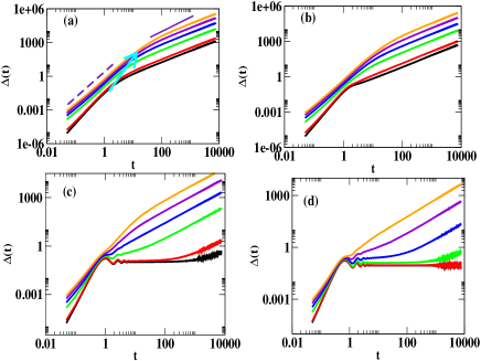
Figure 1: (color online) Plot of MSD, $\Delta(t)$ vs. time $t$ on $\log-\log$ scale, for $\bar{h}=0.0$(a), $\bar{h}=0.1$ (b), $\bar{h}=0.5$ (c),$\bar{h}=1.0$ (d),for the activity $\bar{v_{0}}$=( 0.0 black, 1.0 red, 4.0 green, 6.0 blue, 8.0 violet, 10.0 orange, lines respectively). The dashed and solid lines in (a) have slope 2 and 1 respectively. The arrow shows the increasing crossover time on increasing $\bar{v_{0}}$.

The crossover time increases on increasing $\bar{v_{0}}$. The active nature of particle leads to enhanced persistent motion. Hence MSD can be compared with the result from persistent random walk (PRW) randomwalk , where $\Delta(t)=2d{D_{eff}}t[1-\exp(\frac{-t}{t_{c}})]$, where $t_{c}$ is the crossover time, $D_{eff}$ is the effective diffusivity and $d=2$ is the dimensionality of space. The $t_{c}$ and $D_{eff}$ obtained by fitting the data for MSD with PRW. When we turn on the SU, for $\bar{v_{0}}\geq 8$, dynamics remains ballistic for small time and then it shows a smooth crossover to diffusive behaviour, as shown in Fig. 1(b). But as we increase SU or for fixed SU decrease $\bar{v_{0}}$, MSD shows a plateau for intermediate times, as shown in Fig. 1(c-d). The extend of the plateau increases on increasing SU and decreasing $\bar{v_{0}}$ and for large $\bar{h}\gtrsim 0.8$ and small $\bar{v_{0}}\lesssim 1$, the extend of plateau present for very long time and particle is eventually confined. In Fig.2 (a-b) we plot the scaled MSD, $\frac{\Delta(t)}{4D_{eff}t_{c}}$ vs. scaled time $\frac{t}{t_{c}}$. Data shows the excellent scaling for the flat surface Fig. 2(a), which confirms that on the flat surface, for all values of $\bar{v_{0}}$, the dynamics of particle is like PRW. As shown in Fig. 2(b), motion on the undulated surface shows deviation from scaling, which is due to the transient arrest of particle in surface minima for small $\bar{v_{0}}$. The inset of Fig. 2(b) shows the zoomed plot of deviation from scaling. When two particles are stuck in the same surface minimum, then there is a competition between the activity and repulsion among the particles. and the both encourages the particles to come out. Hence the time spent in a surface minimum or length of the plateau increases on decreasing $\bar{v_{0}}$ and increasing $\bar{h}$. Interaction enhances the particle dynamcis for a fixed activity $\bar{v_{0}}$.

We describe the particle dynamics in simple manner using real space snapshots of a single particle trajectory for fixed $\gamma=1.0$ and $k=1$, in Fig. 3(I-III). Fig. 3(b) shows the cartoon of part of surface. The dark and bright colors show the surface minima and maxima respectively.

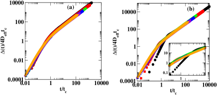
Figure 2: (color online) Plot of the scaled MSD, $\frac{\Delta(t)}{4D_{eff}t_{c}}$ vs. scaled time $\frac{t}{t_{c}}$ on $\log-\log$ scale, for different $\bar{h}=0.0$ (a),$\bar{h}=0.1$ (b) for the same activities as in Fig. 1(a). (b) (inset) shows the zoomed plot near crossover time $t_{c}$.

For small values of $\bar{v_{0}}\lesssim 1.0$ and $\bar{h}\gtrsim 0.8$, initially, (early time $\sim$ first few steps) motion of particle is ballistic but soon it jumps into one of the minima and stays there (snapshot of particle position for $\bar{h}=1.0,$ and $\bar{v_{0}}=0.0$, as shown in Fig. 3(I). Although, soft repulsive interaction among the particles will be maximum, when more than one particle sit in a minima but they do not come out due to small activity. Hence, MSD remains flat for the late time (as shown in Fig.1(d) (black circles). Increasing $\bar{v_{0}}$, leads to partial trapping of the particle in the minima and particle starts moving from one minima to another after some transient time, as shown in snapshot Fig.3(II) is for $\bar{h}=1.0$ and $\bar{v_{0}}=7.0$. So, after an intermediate time (plateau region) , MSD starts growing linearly with time. Snapshot in Fig. 3(III) for $\bar{h}=1.0$ and $\bar{v_{0}}=10.0$. It shows the, particle’s frequent jumps from one minimum to another.

We further investigate the dynamics of particle by extracting the dynamic MSD exponent $\beta(t)$, defined by $\Delta(t)\sim t^{\beta(t)}$, hence $\beta(t)$ can be obtained by assuming MSD, $\Delta(t)\sim t^{\beta(t)}$. Hence $\Delta(10t)\sim(10t)^{\beta(t)}$, hence $\beta(t)$ can be obtained from the ratio of logarithmic (base 10) of two MSD’s,

$$\beta(t)=\frac{log_{10}[\Delta(10t)]}{log_{10}[\Delta(t)]}$$ (4)

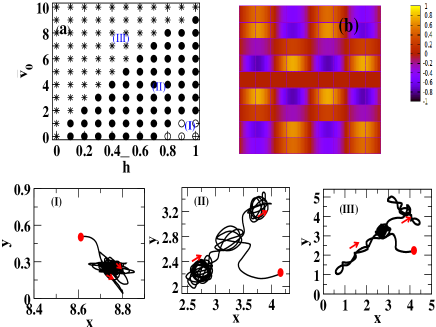
Figure 3: (color online) (a) Phase diagram in the ($\bar{v_{0}}$, $\bar{h}$) plane, region I (open circle), region II (filled circles) and region III (stars), three different phases (C), (SbD) and (SpD) respectively on the linear-linear scale. (b) Cartoon of a part of the surface. The bright blue color and bright yellow color show the location of minima and maxima respectively and color bar shows the height of the surface. (I-III) shows the trajectory of a single particle for parameters $(\bar{v_{0}},\bar{h})$ = $(0.0,1.0),(7,1.0),(10.0,1.0)$ where particle is in three different regions (I)-(III) respectively. For all (I-III) ($t=6000$) time duration of particle trajectory is same and red dot is the location of particle at the start of the trajectory, arrow shows the direction of trajectory after every 2000 times.

Fig. 4(a-d) shows the plot of $\beta(t)$ vs. $t$ for flat and undulated surfaces, $\bar{h}$= $0,0.1,0.2$ and $1.0$ respectively. For all $\bar{v_{0}}$, late time value of $\beta$ either $0$ (confinement) or $1$ (diffusion). Approach to the late time dynamic, depends upon the SU and activity. On the flat surface $\bar{h}=0$, for all activity and greatest $\bar{h}=1.0$, for large $\bar{v_{0}}\geq 10.0$, approach is always through an early time superdiffusion $\beta>1$ to late time diffusion $\beta=1$, but for moderate $\bar{v_{0}}<10.0$, approach to $\beta=1$ is through an intermediate subdiffusive regime, where $\beta<1$. Also for very small activity and large SU ($\bar{v_{0}}\lesssim 1$ and $\bar{h}\gtrsim 0.8$), motion is confined in one of the surface minimum. Hence, the dynamics of particle is of three types: (i) late time confinement $\beta(t)=0$ (C), (ii) approach to diffusion $\beta(t)=1$ from intermediate subdiffusion $\beta(t)<1$ (SbD) and (iii) Initial superdiffusion $\beta(t)>1$ to late time diffusion $\beta(t)=1$ (SpD). Hence for sufficiently large activity $\bar{v_{0}}\gtrsim 1$, the asymptotic dynamics of particle moving on undulated surface is always diffusive, only route to the steady state is different.
We also compared the results for large friction coefficient, when model can be compared with the overdamped dynamics of ABP on undulated surface. We find much slower dynamics for the large friction limit $\gamma=100$ as shown in 5(a-b). We also compared the results for non-interacting $k=0$ and large interaction $k=100$ in Fig. 5(a), where dynamics can be similar to particle moving on strong surface and flat surface respectively. Hence effective dynamics becomes slower and enhanced for the two extreme cases as shown in Fig. 5(b).
Further, we propose that, the underlying surface acts like a medium with an effective temperature, in which particles are moving. To confirm this we compare the effective diffusivities from MSD with the velocity auto-correlation function VACF, $C(t)=<{\bf v}_{i}(t+t_{0})\cdot{\bf v}_{i}(t_{0})>$ using Green-Kubo (GK) relation gk ; gk1 . To our surprise we find that for flat as well as moderate $\bar{h}\lesssim 0.2$, the GK relation is satisfied for all values of $\bar{v_{0}}\in(0,10.0)$. Details of our study we discuss next.

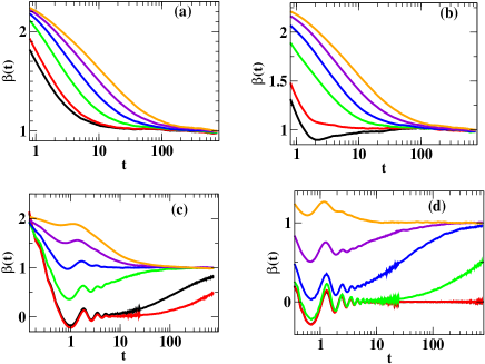
Figure 4: (color online) (a-d) Plot of the dynamic MSD exponent $\beta(t)$ vs. time $t$ on $\log-linear$ scale, for different $\bar{h}$ and $\bar{v_{0}}$ same as in Fig. 1(a).

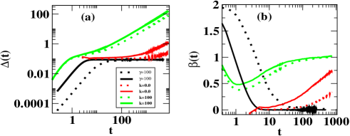
Figure 5: (color online) Plot of the MSD (a), $\beta(t)$ vs. time $t$ on $\log-linear$ scale for plot (a) in (b), different value of $k$ and $\gamma$, dotted and solid line repectively for $\bar{v_{0}}=0.0,1.0$ .

III.1 Green-Kubo relation

Table 1: Comparison of diffusivity from MSD and VACF

$\bar{v_{0}}$	$\Delta D_{eff}(\bar{h}=0.0)$	$\Delta\mathcal{D}(\bar{h}=0.0)$	$\Delta D_{eff}(\bar{h}=0.1)$	$\Delta\mathcal{D}(\bar{h}=0.1)$	$\Delta D_{eff}(\bar{h}=0.2)$	$\Delta\mathcal{D}(\bar{h}=0.2)$
1	0.811$\pm$0.002	0.82$\pm$0.0046	1.12$\pm$0.006	1.09$\pm$0.003	1.90$\pm$0.006	1.86$\pm$0.006
2	2.25$\pm$0.008	2.45$\pm$0.008	3.37$\pm$0.0028	3.63$\pm$0.015	6.41$\pm$0.006	5.95$\pm$0.009
3	5.27$\pm$0.019	5.51$\pm$0.013	7.87$\pm$0.008	7.90$\pm$0.01	17.06$\pm$0.001	15.08$\pm$0.004
4	11.09$\pm$0.03	11.41$\pm$0.028	14$\pm$0.015	16.27$\pm$0.017	37.7$\pm$0.004	34.65$\pm$0.01
6	36.69$\pm$0.013	40$\pm$0.064	63.37$\pm$0.05	63.18$\pm$0.02	169.96$\pm$0.019	154.21$\pm$0.041
8	113.18$\pm$0.09	113.51$\pm$0.065	210.25$\pm$0.25	206.36$\pm$0.38	650.61$\pm$0.12	593.78$\pm$0.05
10	266.90$\pm$0.34	265.31$\pm$0.39	551$\pm$0.19	530$\pm$0.26	2011.9$\pm$0.25	1857.26$\pm$0.2

We first measure the VACF for the flat and different SUs. The VACF decays exponentially to zero on the flat surface, $C(t)=C_{0}(\exp(-t/\tau)$, where $C_{0}$ is the correlation for $t=0$ and $\tau$ is the decay time and it increases with increasing activity. On undulated surface, after the initial exponential decay, the VACF oscillates about zero. The oscillations are due to periodic trapping and untrapping of particle due to finite depth of the surface. We estimate the decay time $\tau$ from the exponential decay. In Fig. 6 (a-b) we plot the scaled VACF, $C(t)/C_{0}$ vs. scaled time $t/\tau$ for flat surface and for $\bar{h}=0.1$. Data shows nice scaling collapse for all $\bar{v_{0}}$ on the flat surface. But on the undulated surface, it deviates at late times, due to periodic oscillations in VACF. Now we assume an effective equilibrium and calculate the diffusivity $\mathcal{D}(\bar{v_{0}},\bar{h})$ by the late time $\lim_{t\rightarrow\infty}\frac{\int_{0}^{t}(<v(t^{\prime})v(0)>)dt^{\prime}}{d}$, where $d$ is dimensionality of the space. We further compare it with the effective diffusivity calculated from MSD, $D_{eff}(\bar{v_{0}},\bar{h})=lim_{t\rightarrow\infty}\frac{\Delta(t)}{2dt}$.

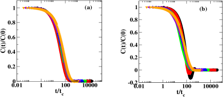
Figure 6: (color on line) Plot of the scaled VACF for (a) $\bar{h}=0.0$ and (b) $\bar{h}=0.1$, on the log-linear scale. The other parameters are same as in Fig. 2.

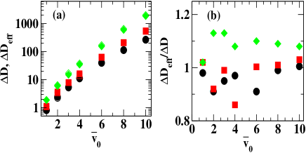
Figure 7: (color online) Comparison plot of the two relative diffusivities from MSD and VACF, $\Delta D_{eff}$ and $\Delta\mathcal{D}$ respectively with respect to $\bar{v_{0}}$. Open and filled symbols are for $\Delta D_{eff}$ and $\Delta\mathcal{D}$ respectively. The three symbols (circles, squares and diamonds) are for three different $\bar{h}=0.0$ and $\bar{h}=0.1$ and $\bar{h}=0.2$ respectively. Plot (b) shows $\Delta D_{eff}$/$\Delta\mathcal{D}$ ratio of diffusivities from MSD and VACF. Error bars are of the order of symbol size.

Fig. 7 shows the plot of the comparison between the two relative diffusivities from MSD and VACF on the linear-log scale, $\Delta D_{eff}=\frac{(D_{eff}(\bar{h},\bar{v_{0}})-D_{eff}(\bar{h},0))}{D_{eff}(\bar{h},0)}$ and $\Delta\mathcal{D}=\frac{(\mathcal{D}(\bar{h},\bar{v_{0}})-\mathcal{D}(\bar{h},0))}{\mathcal{D}(\bar{h},0)}$ vs. $\bar{v_{0}}$ respectively, for three different $\bar{h}=0,0.1$ and $0.2$. The $D_{eff}(\bar{h},0)/\mathcal{D}(\bar{h},0)$ is the diffusivity for zero $v_{0}$ or for passive system. It is larger on the flat surface and decreases on increasing $\bar{h}$. In the table 1 we list the two relative diffusivities for flat $\bar{h}=0.0$ and undulated surface $\bar{h}=0.1$ and $0.2$. On the flat surface the two relative diffusivities shows good match and hence GK relation is satisfied. On the undulated surface, for smaller $\bar{v_{0}}$, data shows good match for all $\bar{v_{0}}$ and $\bar{h}$. Hence for small $\bar{v_{0}}$ and $\bar{h}$ an effective equilibrium is found in this nonequilibirum system. Fig. 7(b) shows the comparison (ratio) plot of the two relative diffusivities form MSD and VACF. As it is very clear for all $\bar{v_{0}}$, data for ratio fluctuates around 1, and approach to 1, for larger $\bar{v_{0}}$. Any deviation we find is due to partial trapping of particle in surface. For small $\bar{v_{0}}$, time spend in trapped state or plateau is longer hence more deviation from GK relation. Hence in such active system an effective equilibrium can be establsihed with respect to relative diffusivity as in corresponding passive system.

IV Discussion

We have studied the dynamics and steady state of a collection of AP moving on a two-dimensional periodically undulated surface. The activity of the particle is present due to an internal energy mechanism, which introduces an active friction sg , which enhances the particle motion when it slows down and suppresses the motion when it tries to accelerate. The activity $\bar{v_{0}}$ and SU $\bar{h}$ are the two control parameters of the system. On the flat surface, $\bar{h}=0$, dynamics of the particle is like PRW with initial ballistic to late time crossover to diffusion. The crossover time increases by increasing $\bar{v_{0}}$. On the undulated surface we find a systematic deviation from PRW and particle shows the transient arrest in different surface minima. Due to this, the MSD shows a plateau for small $\bar{v_{0}}$ and larger $\bar{h}$. The particle shows the three types of motion: (i) confined (C), (ii) from initial subdiffusion to late time diffusion (SbD) and (iii) initial superdiffusion to late time diffusion (SpD). We draw a phase diagram in the plane of ($\bar{v_{0}}$, $\bar{h}$). Hence final state and route to the late time dynamics of the particle very much depend on its activity and surface characteristics.
Although the system is highly nonequilibrium, we find that for moderate $\bar{h}\lesssim 0.2$ the Green-Kubo relation is satisfied between the effective diffusivity and velocity auto-correlation function.
Our study provides a phase diagram for AP moving under active friction. For finite activity the late time dynamics is diffusive, but route to diffusion is different and depends on surface characteristics and activity. Whereas on the flat surface motion is always like PRW. Hence our study provide the characteristics of AP moving on periodic surface. Our work shows that different types of motion can be generated by tuning the surface and particle interaction. Hence these results can be used for various technological and pharmaceutical applications of AP.
The current study is limited for the periodic surface, it will be interesting to find the behaviour of particles on the surface with random maxima and minima which is present in many biological systems biological .

Acknowledgement
We thank Paramshivay supercomputing center facility at I.I.T.(BHU) Varanasi. VS thanks DST INSPIRE(INDIA) for the research fellowship. S. M. thanks DST,SERB(INDIA),project no. ECR/2017/000659 for partial financial support.
Author contribution statement VS and SM designed the project. VS and SM developed the numerical code, and VS executed it. VS and SM contributed equally. VS, SM and SD contributed in analysing the result and preparing the manuscript.

References

- (1) S. Ramaswamy, Annu. Rev. Condens. Matter Phys.,1,323(2010).
- (2) M. C. Marchetti, J. F. Joanny, S. Ramaswamy, T. B. Liverpool, J. Prost, Madan Rao, R. Aditi Simha, Rev. Mod. Phys.,85, 1143(2013).
- (3) P. Romanczuk, M. Bär, W. Ebeling, B. Lindner, L. Schimansky-Geier, Eur. Phys. J. ST,1 202(2012).
- (4) C. Bechinger, R. D. Leonardo,H. Lowen, C. Reichhardt, G. Volpe,G. Volpe, Rev. Mod. Phys.,88, 045006(2016).
- (5) D.Dell’Arciprete, M. L. Blow, A.T. Brown, F.D.C. Farrell, J.S.Lintuvuori, F.F.McVey, D. Marenduzzo, W.C.K. Poon, Nature Communications,9, 4190(2018).
- (6) E. Rauch, M. Millonas, D. Chialvo,Phys. Lett. A,207, 185(1995).
- (7) A. Cavagna, I. Giardina ,Annual Review of Condensed Matter Physics, 5, 183-207(2014).
- (8) Y. Fily,M. C. Marchetti, Phys. Rev. Lett.,108, 235702(2012).
- (9) J. Tailleur, M. E. Cates, Phys. Rev. Lett., 100, 218103 (2008).
- (10) M. E. Cates, J. Tailleur, Annu. Rev. Condens. Matter Phys., 6, 219(2015).
- (11) M. E. Cates, J. Tailleur, EPL (Europhysics Letters), 101, 2(2013).
- (12) I. Buttinoni, J. Bialké, F. Kümmel, H. Löwen, C. Bechinger, T. Speck, Phys. Rev. Lett. 110, 238301 (2013)
- (13) J. Hu, A. Wysocki, R. G. Winkler, G. Gompper,Scientific Reports, 5,9586 (2015)
- (14) J. Palacci, S. Sacanna, A.P. Steinberg, D. J. Pine, P. M. Chaikin, Science 339, 936 (2013)
- (15) M. Paoluzzi, R. Di Leonardo, L Angelani, J. Phys. Condens. Matter 26 375101 (2014)
- (16) P. Dolai, A. Simha, S. Mishra, Soft Matter,14, 6137-6145(2018).
- (17) J. Toner, Y. Tu, Phys. Rev. Lett.,75 4326(1995).
- (18) J. Toner, N. Guttenberg, Y. Tu, Phys. Rev. E, 98, 062604(2018).
- (19) G. S. Redner, M. F. Hagan, A. Baskaran, Phys. Rev. Lett., 110, 055701(2013).
- (20) R. Wittkowski, A. Tiribocchi, J. Stenhammar, R. Allen, D. Marenduzzo, M. E. Cates, Nat. Comm., 5, 4351(2014).
- (21) P. Digregorio, D. Levis, A. Suma, L. F. Cugliandolo, G. Gonnella I. Pagonabarraga, Phys. Rev. Lett. 121 098003, (2018).
- (22) M. Paoluzzi, C. Maggi, A.Crisanti, Phys. Rev. R. 2 023207,(2020).
- (23) M. Mijalkov, A. McDaniel, J. Wehr, G. Volpe, Phys. Rev. X,6, 011008(2016).
- (24) U. Choudhury, A. V Straube, P. Fischer, J. G Gibbs, F. Hofling, New Journal of Physics, 19, 125010(2017).
- (25) M Pelton, K Ladavac, D G Grier, Phys. Rev. E, 70, 031108(2004).
- (26) S. Pattanayak, R. Das, M. Kumar, S. Mishra, The European Physical Journal E, 42 62(2019).
- (27) X. Ao, P. K. Ghosh, Y. Li, G. Schmid, P. Hänggi, F. Marchesoni, EPL (Europhys. Lett.),109, 10003(2015).
- (28) D. Ray, C. Reichhardt, C. J. Olson Reichhardt, Phys. Rev. E, 90, 013019(2014).
- (29) F. Kmmel, B. t. Hagen, R. Wittkowski, I. Buttinoni, R. Eichhorn, G. Volpe, H. Lowen, C. Bechinger, Phys. Rev. Lett., 110, 198302(2013).
- (30) C. Maggi, J. Simmchen, F. Saglimbeni, J. Katuri, M. Di- palo, F. De Angelis, S. Sanchez, R. Di Leonardo, 2016, Small, 12, 446–451.
- (31) N. Kumar, R.K. Gupta, H. Soni, S. Ramaswamy, A.K. Sood Phys. Rev. E, 99 ,032605(2019).
- (32) A. Kaiser, H. H. Wensink, H. Löwen, Phys. Rev. Lett., 108, 268307(2012).
- (33) W. Ebeling, E. Gudowska, A. Fiasconaro, Acta Physica Polonica B, 39,1251(2008).
- (34) F. Schweitzer, W. Ebeling, B. Tilch, Phys. Rev. E, 64, 021110(2001).
- (35) U. Erdmann, W. Ebeling, L. Schimansky-Geier, F. Schweitzer,Euro. Phys. J. B, 15, 105-113(2000).
- (36) F. Peruani, I. S. Aranson, Phys. Rev. Lett. 120 238101(2018)
- (37) J. Masoliver, K. Lindenberg, G. H. Weiss, Physica A, 157 (2), 891–898(1989).
- (38) K. Franke, H. Gruler, Europ. Biophys. J., 18, 335(1990).
- (39) H. Gruler, B. Bültmann, Blood Cells, 10, 61-77(1984).
- (40) . A. d. Boisfleury-Chevance, B. Rapp, H. Gruler, Blood Cells, 15, 315-33(1989).
- (41) H. Gruler, R. Nuccitelli, Cell Mot. Cytoskel, 19, 121(1991).
- (42) M. Schienbein, H. Gruler, Bulletin of Mathematical Biology, 55,585–608(1993).
- (43) G.E.Uhlenbeck, L.S.Ornstein, Physical Review, 36, 823(1930).
- (44) W. C. Swope, H. C. Andersen J. Chem. Phys., 76, 637(1982).
- (45) N. S.Martys, R. D. Mountain, Phys. Rev. E, 59,3733(1999).
- (46) M. Zeitz, K. Wolff, H. Stark, Eur. Phys. J. E,40, 23(2017).
- (47) M. S. Green, J. Chem. Phys., 22, 398(1954).
- (48) R. Kubo, M. Yokota, S Nakajima, J. Phys. Soc. Jpn., 12, 1203-1211(1957).
- (49) C. Battle, C. P. Broedersz, N. Fakhri,V. F. Geyer, J. Howard, C. F. Schmidt, F. C. MacKintosh, Science, 352,604-607(2016).