Abstract

The aim of this analysis was to determine whether or not the given error bars truly represented the dispersion of values in a historical compilation of two cosmological parameters: the amplitude of mass fluctuations ($\sigma_{8}$) and Hubble’s constant ($H_{0}$) parameters in the standard cosmological model. For this analysis, a chi-squared test was executed on a compiled list of past measurements. It was found through analysis of the chi-squared ($\chi^{2}$) values of the data that for $\sigma_{8}$ (60 data points measured between 1993 and 2019 and $\chi^{2}$ between 182.4 and 189.0) the associated probability Q is extremely low, with $Q=1.6\times 10^{-15}$ for the weighted average and $Q=8.8\times 10^{-15}$ for the best linear fit of the data. This was also the case for the $\chi^{2}$ values of $H_{0}$ (163 data points measured between 1976 and 2019 and $\chi^{2}$ between 480.1 and 575.7), where $Q=1.8\times 10^{-33}$ for the linear fit of the data and $Q=1.0\times 10^{-47}$ for the weighted average of the data. The general conclusion was that the statistical error bars associated with the observed parameter measurements have been underestimated or the systematic errors were not properly taken into account in at least 20% of the measurements. The fact that the underestimation of error bars for $H_{0}$ is so common might explain the apparent 4.4$\sigma$ discrepancy formally known today as the Hubble tension.

xx 1 5 Received: date; Accepted: date; Published: date yes A Chi-Squared Analysis of the Measurements of Two Cosmological Parameters Over Time Timothy Faerber ¹ and Martín López-Corredoira ^2,3,* Timothy Faerber and Martín López-Corredoira Correspondence: fuego.templado@gmail.com

1 Introduction

1.1 The Standard Cosmological Model

The standard cosmological model is a model that aims to describe the evolution and structure of the Universe that we live in. This theoretical model accounts for our Universe’s beginning through inflation caused by the Big Bang all the way up to the present-day dark energy dominated Universe ($\sim$70%). In addition to explaining the evolution and current state of the Universe, the standard cosmological model can be interpreted to predict the Universe’s fate. The standard cosmological model consists of 12 parameters (Croft and Dailey, 2015): $\Omega_{M}$ is the ratio of the current matter density to the critical density, $\Omega_{\Lambda}$ is the cosmological constant as a fraction of the critical density, $H_{0}$ is Hubble’s constant, $\sigma_{8}$ is the amplitude of mass fluctuations, $\Omega_{b}$ is the baryon density as a fraction of the critical density, $n$ is the primordial spectral index, $\beta$ is the redshift distortion, $m_{v}$ is the neutrino mass, $\Gamma$ is $\Omega_{m}H_{0}/100$ kms^-1Mpc^-1, $\Omega_{m}^{0.6}\sigma_{8}$ is a combination of two other parameters that is useful in some peculiar velocity and lensing measurements, $\Omega_{k}$ is the curvature, and $w_{0}$ is the equation of state for the dark energy parameter (Croft and Dailey, 2015). For this study, the two parameters in question are $\sigma_{8}$ and $H_{0}$.

1.2 Amplitude of Mass Fluctuations ($\sigma_{8}$)

The amplitude of mass fluctuations ($\sigma_{8}$) is a parameter in the standard cosmological model that is concerned with the respective distributions of mass and light in the Universe (Fan et al., 1997). This is of interest to cosmologists because if $\sigma_{8}\simeq 1$, the implication is an "unbiased" Universe in which mass and light are evenly distributed in a sphere of radius $R$ = 8 $h^{-1}$ Mpc, whereas if $\sigma_{8}\simeq 0.5$, the result would be a "biased" Universe in which mass is distributed more extensively than light in a sphere of radius $R$ = 8 h^-1 Mpc (Fan et al., 1997). It is important for cosmologists to study and understand the distribution tendencies of mass and light in the Universe through $\sigma_{8}$ because large-scale differences in distribution of matter and energy in the present-day Universe tell us about density fluctuations in the early Universe on the cluster mass scale of $R$ = 8 h^-1 Mpc (Fan et al., 1997).

1.3 Hubble’s Constant ($H_{0}$)

Hubble’s constant ($H_{0}$), like the amplitude of mass fluctuations, is a parameter in the standard cosmological model.

$H_{0}$ is the slope of the line in the Hubble–Lemaître Law, relating the recession velocity of a galaxy to the distance that it is from an observer. A representation of this law can be seen in Figure 1, obtained from Paturel et al. (2017). In other words, $H_{0}$ relates to the expansion of the Universe on cosmic scales and is named after Edwin Hubble who discovered it in 1929 when he realized that galaxies’ velocities away from an observer are directly proportional to their distance from that observer, except for cases of peculiar velocities (Kragh and Smith, 2003). In recent years however, credit has also been given to Georges Lemaître jointly with Hubble for the discovery of this relationship (Elizalde, 2019). The parameter is measured in km s^-1 Mpc^-1 and describes the velocity with which a galaxy of distance $d$ from an observer is moving radially away from that observer. Since the Universe is so large, these recession velocities in the form of redshift ($z$) are used to describe the distances to far away galaxies rather than units of length. Knowing the exact value of $H_{0}$ is important to cosmologists, as $H_{0}$ can also be used to roughly calculate the age of the Universe.

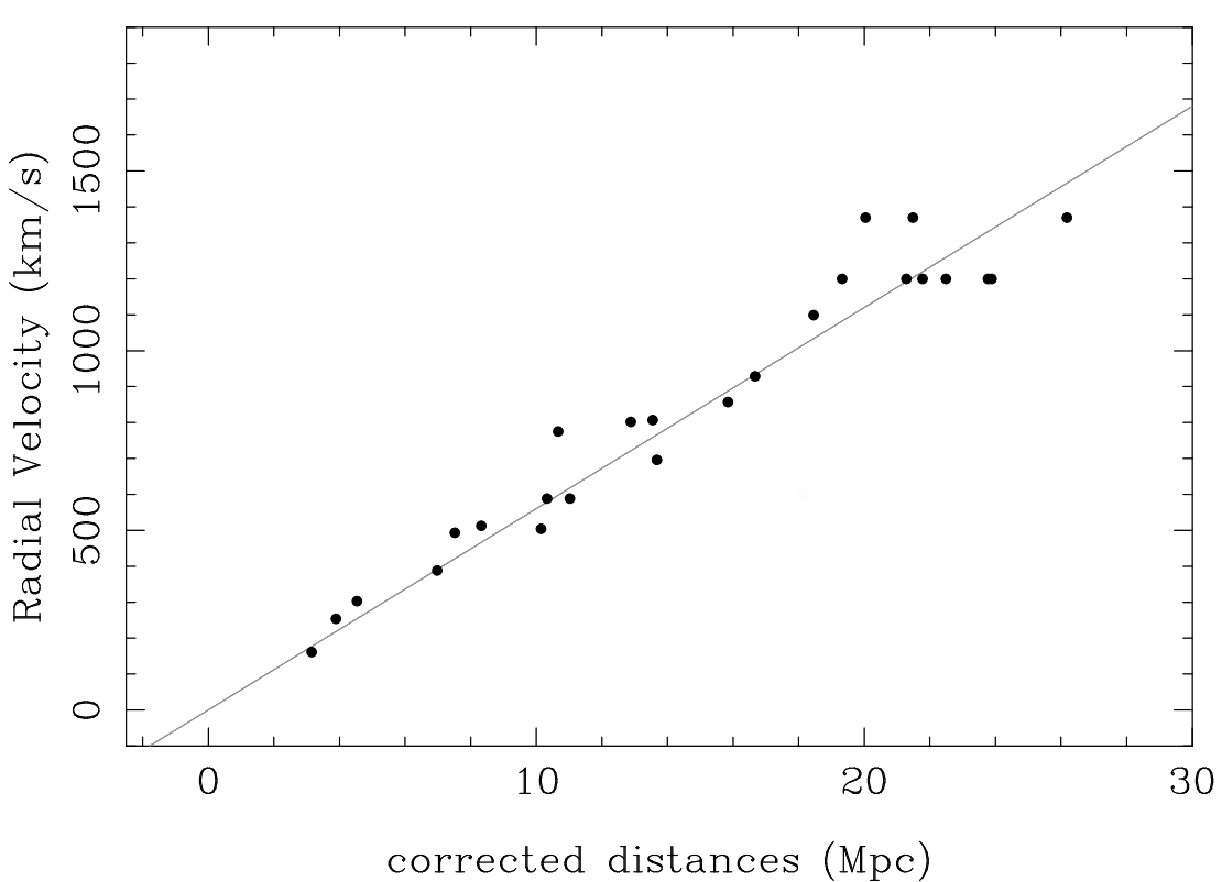
Figure 1: The Hubble–Lemaître Law (Elizalde, 2019) representing radial recession velocity vs. distance from observer.

1.4 Values and Errors

The first step in the process of determining the best observed values for the amplitude of mass fluctuations parameter ($\sigma_{8}$) and Hubble’s constant ($H_{0}$) was to compile a list of several tens of measurements of these parameters. For this specific project, 60 values were compiled for $\sigma_{8}$ between the years of 1993 and 2019 and 163 values were compiled for $H_{0}$ between the years of 1976 and 2019. In addition to the values themselves, we were interested in a few other details about the measurements, namely, the years that those measurements were made in and the sizes of the error bars corresponding to the observed values. A list of all 60 observed measurements for $\sigma_{8}$ 163 observed values for $H_{0}$ can be found in Tables 2 and 7, respectively, in the Appendix. For $H_{0}$ values (units throughout this paper in km s¹ Mpc^-1) between 1990 and 2010; all of the values stem from Croft and Dailey (2015). These tables include the observed values along with their years of observation, sizes of error, and references to source articles. All of the referenced papers were found using the Astrophysics Data System (https://ui.adsabs.harvard.edu/), or from the tables in Croft and Dailey (2015). For the statistical analysis of this data, a simplifying assumption was made that each observed measurement is independent of the other observed measurements, eliminating the need for a covariance term. It should also be noted that the given error bars account for all statistical effects.

2 Statistical Analysis

2.1 Chi-Squared Test

In order to analyze the trends in our datasets when viewed in scatter plots (see Figures 2 and 3), a good statistical test is a chi-squared test. We used a chi-squared test to examine the probabilities of the deviations and determine whether the simplifying assumption made that the measurements were independent of one another was correct.

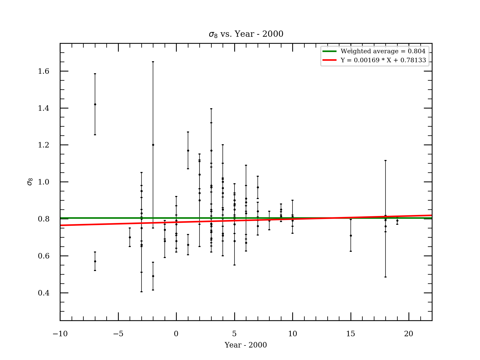
Figure 2: Data of $\sigma_{8}$ vs. time (year—2000) data, weighted average, and best linear fit.

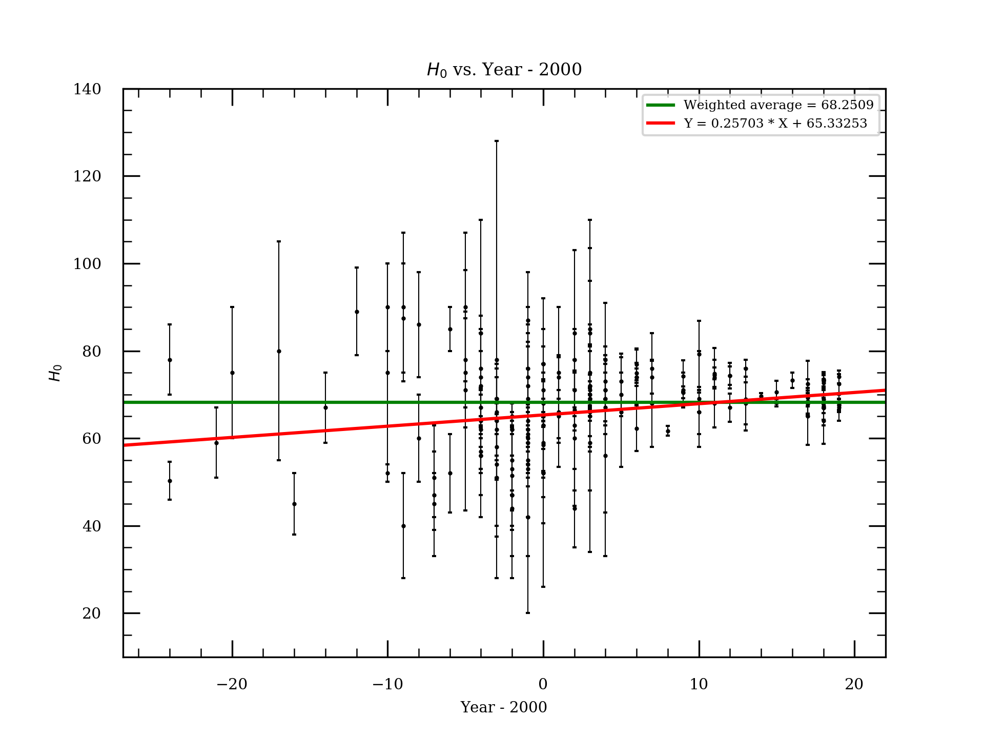
Figure 3: Data of $H_{0}$ vs. time (year—2000) data, weighted average, and best linear fit.

The chi-squared value of a set of data gives the likelihood that the trend observed in the data occurred due to chance, and is also known as a "goodness of fit" test (Plackett, 1983). The chi-squared value of a dataset is given by the following expression:

$$\chi^{2}=\sum_{i=1}^{N}\frac{(x_{n,i}-x_{t,i})^{2}}{\sigma^{2}_{i}},$$ (1)

where in the case of our dataset $x_{n,i}$ is the observed value for the parameter, $x_{t,i}$ is the theoretical value for the parameter (weighted average or linear fit), $\sigma^{2}_{i}$ is the variance of the observed parameter value, and $N$ is the number of points. The term for covariance term is absent from this expression due to the simplifying expression made that all of the observed measurements are independent of one another. This independence of data is precisely the hypothesis we want to test. If the data were not independent, we would have to add a term for covariance to Equation (1). In any case, non-independency of our data would make the spread of the points lower than is indicated by the error bars, making the probability $Q$ (see Section 2.3) of higher deviations even lower, and thus number of points to reject in order to have a distribution compatible to the error bars even larger. Therefore, our simplified approach can be considered a conservative calculation.

This calculation was carried out twice, first using the weighted average $\sigma_{8}$ and $H_{0}$ values as the theoretical values ($x_{t}$), and then again using the best fit values from a linear fit designed to minimize the value of $\chi^{2}$ as $x_{t}$. Lines representing both the weighted average of the dataset (blue) and the best fit for the dataset (red) that were used to calculate chi-squared can be seen with the data points in Figures 2 and 3. The weighted averages ($\lambda_{w}$) of the parameters in question were calculated by weighting each point by the variance of that value, as shown below, where $\sigma^{2}_{i}$ is the variance of data point $i$:

$$\lambda_{w}=\frac{\sum_{i=1}^{n}\frac{x_{i}}{\sigma^{2}_{i}}}{\sum_{i=1}^{n}\frac{1}{\sigma^{2}_{i}}}$$ (2)

For $\sigma_{8}$, $\lambda_{w}\approx 0.8038$ and for $H_{0}$, $\lambda_{w}\approx 69.3815$. Substituting these weighted averages in for $x_{t}$ in Equation (1) gives $\chi^{2}\approx 189.037$ for $\sigma_{8}$ and $\chi^{2}\approx 575.655$ for $H_{0}$.

In order to find the linear fit of the form:

$$Y=A+B\times X$$ (3)

where $Y$ is the theoretical value for the parameter being analyzed and $X$ is the year of that measurement minus 2000. A program was written in Python that minimizes $\chi^{2}$. When replacing $Y$ from Equation (4) for $x_{t}$ in Equation (1), we found that $\chi^{2}\approx 182.4$ for $\sigma_{8}$ and $\chi^{2}\approx 480.1$ for $H_{0}$. In order to calculate the error bars for the parameters A and B, a program was written in Python to estimate the range of values for $\sigma_{8}$ and $H_{0}$ with an error of 1$\sigma$ added. The 1$\sigma$ error (68% C.L.) was obtained by adding the value of $2.3\left(\frac{\chi^{2}}{n}\right)$ to the minimum of $\chi^{2}$ values of 182.4 ($\sigma_{8}$) and 480.1 ($H_{0}$) in accordance to the process followed in Avni (1976), where $n$ is the number of degrees of freedom and the second factor was added to account for either under or overestimation of the error bars. For our $\sigma_{8}$ values, this process resulted in an A value of $0.781\pm 0.012$ and a $B$ value of $(1.7\pm 0.8)\times 10^{-3}$. With these values for $A$ and $B$, the function of the linear fit for $\sigma_{8}$ becomes:

$$Y=0.781+(1.7\times 10^{-3})\times X$$ (4)

For the $H_{0}$ values, this process resulted in an $A$ value of $65.3\pm 0.6$ and a $B$ value of $0.26\pm 0.04$, making the function of the linear fit for $H_{0}$:

$$Y=65.3+0.26\times X$$ (5)

as can be seen in Figures 2 and 3, represented by the red line.

2.2 Reduced Chi-Squared

In order to account for the degrees of freedom in the data, a reduced chi-squared test was used to test the goodness of fit for both the weighted average and best fit values. Reduced chi-squared is commonly used for several purposes in astronomy, namely, model comparison and error estimation (Andrae et al., 2010). The reduced chi-squared value of a dataset is simply the chi-squared value divided by the degrees of freedom ($n$) of that dataset, as shown in the following relation:

$$\chi^{2}_{n}=\frac{\chi^{2}}{n}$$ (6)

In the case of this analysis, for the weighted average calculations there were 59 degrees of freedom for $\sigma_{8}$ and 162 degrees of freedom for $H_{0}$ (one free parameter). For the linear fit calculations there were 58 degrees of freedom for $\sigma_{8}$ and 161 degrees of freedom for $H_{0}$ (two free parameters). When applying the $\chi^{2}$ value calculated using the weighted average of the dataset to Equation (5), we get a reduced chi-squared (or, chi-squared per degree of freedom) of 3.20 for $\sigma_{8}$ and a reduced chi-squared value of 3.55 for $H_{0}$. Likewise, the reduced chi-squared value obtained from the best fit function meant to minimize reduced chi-squared is 3.04 for $\sigma_{8}$ and is 2.95 for $H_{0}$, both of which, in accordance to theory, are less than those calculated using the weighted average (0.16 difference for $\sigma_{8}$ and 0.60 for $H_{0}$).

2.3 Statistical Significance, Q

The probability that a calculated $\chi^{2}$ value for a dataset with $n$ degrees of freedom is due to chance is represented by $Q$ and is given by the following expression:

$$Q_{\chi^{2},n}=[2^{d/2}\Gamma(\frac{d}{2})]^{-1}\int_{\chi^{2}}^{\infty}(t)^{\frac{d}{2}-1}e^{\frac{-t}{2}}dt$$ (7)

where $\Gamma_{x}$ is given by:

$$\Gamma_{x}=\int_{0}^{\infty}t^{x-1}e^{-t}dt$$ (8)

and is known as the generalization of the factorial function to real and complex arguments (Gronau, 2003). In order to determine which values should be removed as bad values, all values were ranked based on their contributions to $\chi^{2}$ by increasing value of [$x-$ (best fit $x$)]/(error of $x$) and then again by [$x-$ (weighted average $x$)]/(error of $x$), where x is the observed value for the parameter in question. Values with the largest contribution to $\chi^{2}$ (bad values) were removed first.

2.3.1 Amplitude of Mass Fluctuations

For the value of $\chi^{2}$ calculated using the weighted average of $\sigma_{8}$ ($n=59,\chi^{2}\approx 189.0$), the probability that the observed trend is due to chance is $Q=1.6\times 10^{-15}$. In order to reach a value for $Q$ that is statistically significant ($Q\geq 0.05$), 14 bad values must be removed from the data ($n=45,\chi^{2}\approx 58.1548$), producing a value for $Q$ of 0.0902. For the value of $\chi^{2}$ calculated using the best fit function designed to minimize $\chi^{2}$ ($n=58,\chi^{2}\approx 182.4$), $Q=8.8\times 10^{-15}$. In order to reach a statistically significant value for $Q$, 10 bad values must be removed from the data ($n=48,\chi^{2}\approx 61.0$), producing a value for $Q$ of 0.099. With this last subsample of 50 points, the best linear fit of $\sigma_{8}$ returned an $A$ value of $0.787\pm 0.008$ and a $B$ value of $(1.1\pm 0.5)\times 10^{-3}$; see Figure 4.

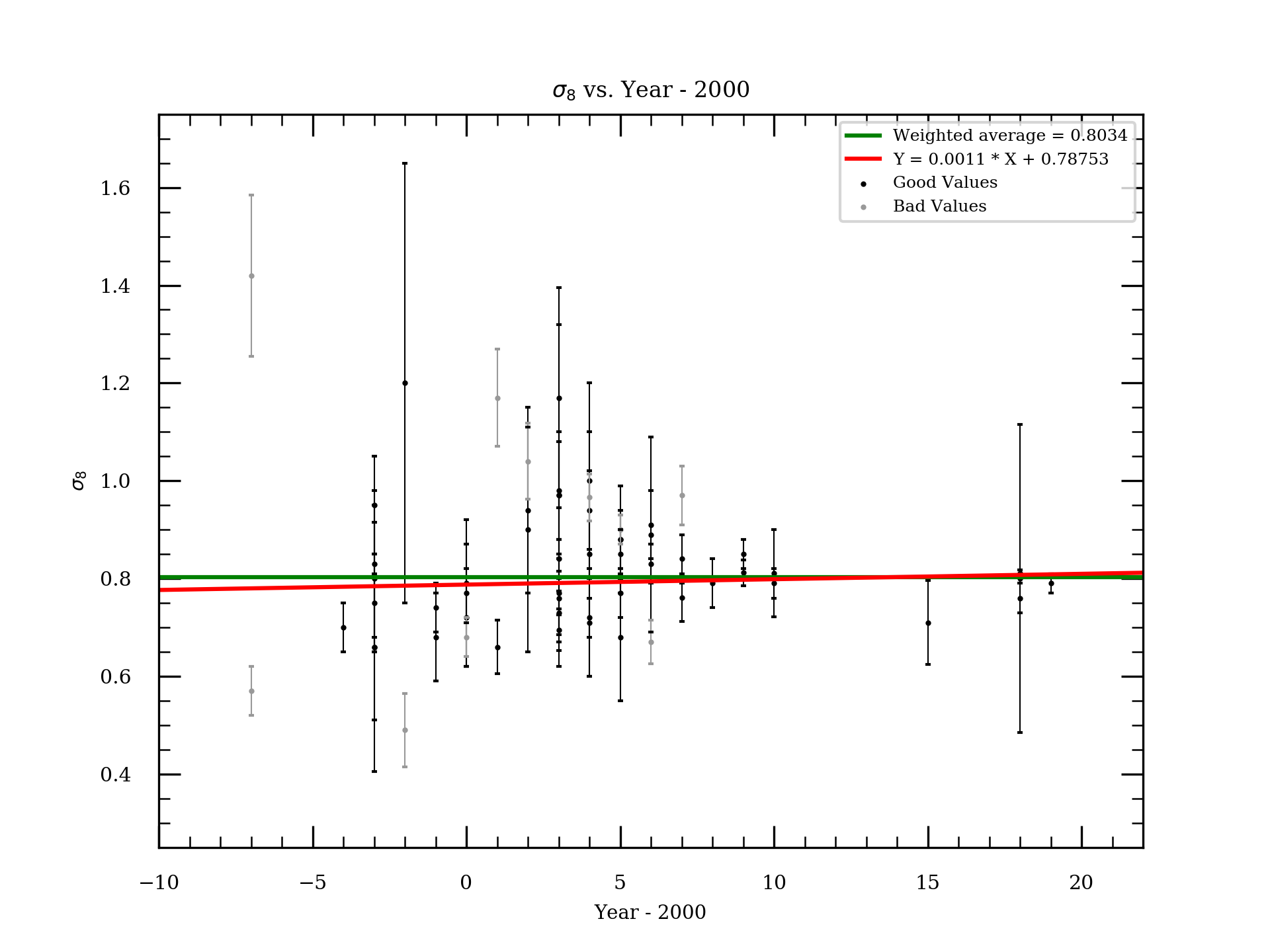
Figure 4: Data of $\sigma_{8}$ vs. time (year—2000) separating the $N=50$ good values that make the $\chi^{2}$ linear fit compatible with the error bars, and the rest of the points ($N=10$) plotted as bad values. Here, we only used the good values for the weighted average and best linear fit.

2.3.2 Hubble’s Constant

For the value of $\chi^{2}$ calculated using the weighted average of $H_{0}$ ($n=162,\chi^{2}\approx 575.655$), the probability that the observed trend is due to chance is $Q=1.0\times 10^{-47}$. In order to reach a value for $Q$ that is statistically significant ($Q\geq 0.05$), 36 bad values must be removed from the data ($n=125,\chi^{2}\approx 152.5541$), producing a value for $Q$ of 0.0538. For the value of $\chi^{2}$ ($n=161,\chi^{2}\approx 480.1$) calculated using the best fit function designed to minimize $\chi^{2}$, $Q=1.8\times 10^{-33}$. In order to reach a statistically significant value for $Q$, 24 bad values must be removed ($n=137,\chi^{2}\approx 164.1$), producing a value for $Q$ of 0.057. With this last subsample of 139 points, the best linear fit of $H_{0}$ returned an $A$ value of $65.9\pm 0.4$ and a $B$ value of $0.277^{+0.032}_{-0.034}$; see Figure 5.

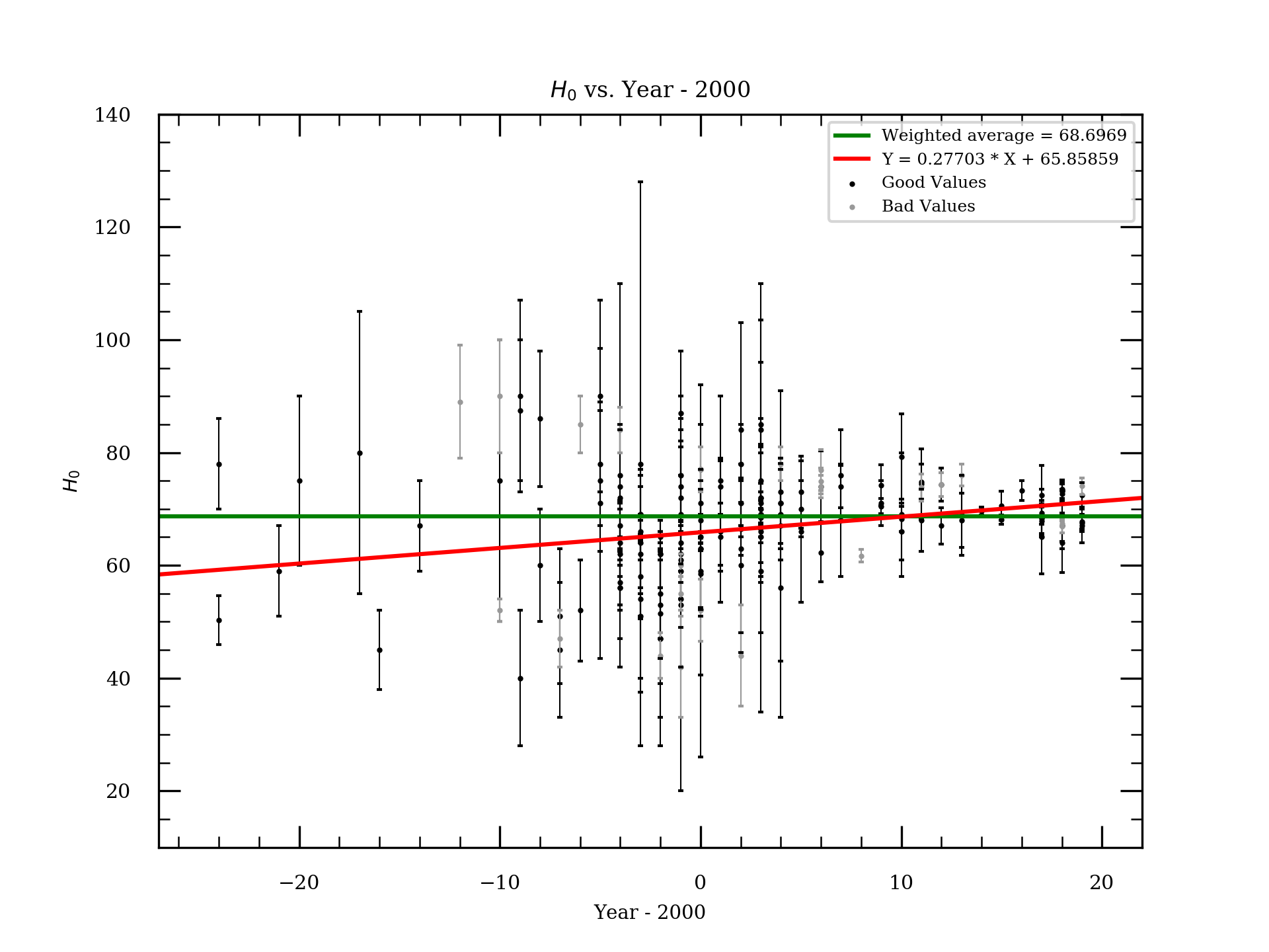
Figure 5: Data of $H_{0}$ vs. time (year—2000) separating the $N=139$ good values that make the $\chi^{2}$ linear fit compatible with the error bars, and the rest of the points ($N=24$) plotted as bad values. Here, we only use the good values for the weighted average and best linear fit.

The non-zero value of $B$ is very significant; however, the error of $B$ may be non-Gaussian and we cannot directly interpret this as significant evolution. The correlation factor of $H_{0}$ with time is $c=0.027\pm 0.013$, a $2\sigma$ significant correlation.

3 Conclusions and Discussion

The original $Q$ values for both the weighted average and best fit calculations of the probability of the data for both parameters are extremely low before the removal of bad values. Even though this is the case, a rather large discrepancy can be seen in how many bad values need removing to reach a statistically significant dataset ($Q\geq 0.05$). For the $\sigma_{8}$ values, to attain statistical significance, the weighted average calculation needs 14 bad values removed, whereas the best fit calculation needs only 10 bad values removed. For the $H_{0}$ values, to attain statistical significance, the weighted average calculation requires 36 bad values be removed, whereas the best fit calculation only needs 24 bad values removed. With the studies of both parameters ending in the aforementioned conclusions, it is reasonable to conclude that the linear fit with time (year—2000) on the $x-$axis and measurements of the parameters in question ($\sigma_{8}$ and $H_{0}$) on the $y-$axis is a better estimation of the data than the weighted averaged of the data weighted with the inverse square proportion of the error of each value in question, a linear fit is a better estimate of the data than the weighted average.

For $H_{0}$, we observed a slight growing trend (at 2-$\sigma$ level) in the value of the measurements in the last 43 years, although the interpretation of this upward trend as a random fluctuation is not excluded.

In addition to the increasing precision of measurements, it is concluded from this analysis that the error bars of the observed parameters have been largely underestimated in at least 20% of the measurements, or the systematic errors of the observation techniques were not fully considered. It should also be stated that, due to the simplifying assumption about the covariance of each observed measurement, 20% of the error bars being underestimated is a conservative percentage (in reality, it is a minimum of 20% the measurements). In the light of the analysis carried out in this paper, one would not be surprised to find cases like the 4.4$\sigma$ discrepancy seen between the best measurement using Supernovae Ia in Riess et al. (2019) of $H_{0}$ = $74.03\pm 1.42$ km s^-1 Mpc^-1 and the value derived from cosmic microwave background radiation of $H_{0}$ = $67.4\pm 0.5$ km s^-1 Mpc^-1. It is likely that the underestimation of error bars for $H_{0}$ in many measurements contributes to the apparent 4.4$\sigma$ discrepancy formally known as the Hubble tension.

Conceptualization, T.F. and M.L.-C.; methodology, M.L.-C.; software, T.F.; formal analysis, T.F.; writing—original draft preparation, T.F.; writing—review and editing, M.L.-C.; supervision, M.L.-C. All authors have read and agreed to the published version of the manuscript.

MLC was supported by the grant PGC-2018-102249-B-100 of the Spanish Ministry of Economy and Competitiveness (MINECO).

Appendix A Tables of Data

Table 1: $\sigma_{8}$ data.

Date	$\sigma_{8}$	$\pm$	Reference
1993	0.57	0.05	White et al. (1993)
1993	1.415	0.165	White et al. (1993)
1996	0.7	0.05	Taylor and Hamilton (1996)
1997	0.75	0.1	Carlberg et al. (1997)
1997	0.95	0.1	Carlberg et al. (1997)
1997	0.8	0.15	Shimasaku (1997)
1997	0.66	$+0.22$ $-0.08$	Henry (1997)
1997	0.66	$+0.34$ $-0.17$	Henry (1997)
1997	0.83	0.15	Fan et al. (1997)
1998	1.2	$+0.5$ $-0.4$	Bahcall and Fan (1998)
1998	0.49	$+0.08$ $-0.07$	Robinson et al. (1998)
1999	0.68	0.09	Einasto et al. (1999)
1999	0.74	0.05	Bridle et al. (1999)
2000	0.72	0.1	Henry (2000)
2000	0.77	0.15	Henry (2000)
2000	0.79	0.08	Matsubara et al. (2000)
2000	0.68	0.04	McDonald et al. (2000)
2001	1.17	0.1	Bridle et al. (2001)
2001	0.66	$+0.06$ $-0.05$	Borgani et al. (2001)
2002	0.94	0.17	Refregier et al. (2002)
2002	1.04	0.104	Evrard et al. (2002)

Table 2: Cont.

Date	$\sigma_{8}$	$\pm$	Reference
2002	1.04	0.078	Komatsu and Seljak (2002)
2002	0.9	$+0.3$ $-0.2$	Bahcall et al. (2002)
2003	0.76	0.09	Melchiorri et al. (2003)
2003	0.98	0.1	Bahcall and Bode (2003)
2003	0.73	$+0.06$ $-0.03$	Brown et al. (2003)
2003	1.17	$+0.25$ $-0.2$	Slosar et al. (2003)
2003	0.77	$+0.05$ $-0.04$	Pierpaoli et al. (2003)
2003	0.695	0.042	Allen et al. (2003)
2003	0.84	0.04	Spergel et al. (2003)
2003	0.97	0.13	Bacon et al. (2003)
2003	0.97	0.35	Hamana et al. (2003)
2004	0.966	0.048	Pope et al. (2004)
2004	0.71	0.11	Heymans et al. (2004)
2004	0.72	0.04	Voevodkin and Vikhlinin (2004)
2004	0.85	$+0.38$ $-0.12$	Łokas et al. (2004)
2004	0.94	0.08	Łokas et al. (2004)
2004	1.0	0.2	Chang et al. (2004)
2005	0.90	0.03	Seljak et al. (2005a)
2005	0.88	0.06	Seljak et al. (2005b)
2005	0.68	0.13	Heymans et al. (2005)
2005	0.85	0.05	Pike and Hudson (2005)
2005	0.88	$+0.12$ $-0.10$	Gaztanaga et al. (2005)
2006	0.89	0.2	Eke et al. (2006)
2006	0.77	0.05	Sanchez et al. (2006)
2006	0.91	0.07	Viel and Haehnelt (2006)
2006	0.67	$+0.04$ $-0.05$	Dahle (2006)
2007	0.761	$+0.049$ $-0.048$	Spergel et al. (2007)
2007	0.84	0.05	Benjamin et al. (2007)
2007	0.97	0.06	Harker et al. (2007)
2008	0.79	0.05	Ross et al. (2008)
2009	0.85	$+0.04$ $-0.02$	Henry et al. (2009)
2009	0.812	0.026	Komatsu et al. (2009)
2010	0.79	0.03	Mantz et al. (2010)
2010	0.811	0.089	Hilbert and White (2010)
2014	0.83	0.04	Mantz et al. (2014)
2015	0.710	0.086	Gil-Marín et al. (2015)
2018	0.811	0.006	Aghanim et al. (2018)
2018	0.76	0.03	Salvati et al. (2018)
2018	0.80	0.31	Corasaniti et al. (2018)
2019	0.786	0.02	Kreisch et al. (2019)

Table 3: $\sigma_{8}$ data.

Date	$H_{0}$ (km s-1 Mpc-1)	$\pm$	Reference
1976	78	8	Jaakkola and Le Denmat (1976)
1976	50.3	4.3	Sandage and Tammann (1976)
1979	59	8	Visvanathan and Griersmith (1979)
1980	75	15	Stenning and Hartwick (1980)
1983	80	25	Rubin and Thonnard (1983)
1984	45	7	Jõeveer (1984)
1986	67	8	Gondhalekar et al. (1986)
1988	89	10	Melnick et al. (1988)
1990	90	10	Croft and Dailey (2015)
1990	75	25	Croft and Dailey (2015)
1990	52	2	Croft and Dailey (2015)
1991	90	17	Croft and Dailey (2015)
1991	87.5	12.5	Croft and Dailey (2015)
1991	40	12	Croft and Dailey (2015)
1992	86	12	Croft and Dailey (2015)
1992	60	10	Croft and Dailey (2015)
1993	51	12	Croft and Dailey (2015)
1993	47	5	Croft and Dailey (2015)
1993	45	12	Croft and Dailey (2015)
1994	85	5	Croft and Dailey (2015)
1994	52	9	Croft and Dailey (2015)
1995	93	1	Croft and Dailey (2015)
1995	90	17	Croft and Dailey (2015)
1995	78	11	Croft and Dailey (2015)
1995	75	12.5	Croft and Dailey (2015)
1995	71	27.5	Croft and Dailey (2015)
1996	84	4	Croft and Dailey (2015)
1996	76	34	Croft and Dailey (2015)
1996	74	11	Croft and Dailey (2015)
1996	72	12	Croft and Dailey (2015)
1996	67	4.5	Croft and Dailey (2015)
1996	64	6	Croft and Dailey (2015)
1996	62	9	Croft and Dailey (2015)
1996	57	4	Croft and Dailey (2015)
1996	56	4	Croft and Dailey (2015)
1996	56	9	Croft and Dailey (2015)
1997	78	50	Croft and Dailey (2015)
1997	69	5	Croft and Dailey (2015)
1997	69	8	Croft and Dailey (2015)
1997	66	10	Croft and Dailey (2015)
1997	64	13	Croft and Dailey (2015)

Table 4: Cont.

Date	$H_{0}$ (km s-1 Mpc-1)	$\pm$	Reference
1997	62	7	Croft and Dailey (2015)
1997	58	7.5	Croft and Dailey (2015)
1997	54	14	Croft and Dailey (2015)
1997	51	13.5	Croft and Dailey (2015)
1998	65	1	Croft and Dailey (2015)
1998	62	6	Croft and Dailey (2015)
1998	62	6	Croft and Dailey (2015)
1998	55	8	Croft and Dailey (2015)
1998	53	9.5	Croft and Dailey (2015)
1998	51.5	12.5	Croft and Dailey (2015)
1998	47	19	Croft and Dailey (2015)
1998	47	14	Croft and Dailey (2015)
1998	44	4	Croft and Dailey (2015)
1999	87	11	Croft and Dailey (2015)
1999	76	14	Croft and Dailey (2015)
1999	74	8	Croft and Dailey (2015)
1999	72	9	Croft and Dailey (2015)
1999	69	15	Croft and Dailey (2015)
1999	64	3.75	Croft and Dailey (2015)
1999	62	5	Croft and Dailey (2015)
1999	61	7	Croft and Dailey (2015)
1999	60	2	Croft and Dailey (2015)
1999	59	17	Croft and Dailey (2015)
1999	55	3	Croft and Dailey (2015)
1999	54	5	Croft and Dailey (2015)
1999	53	33	Croft and Dailey (2015)
1999	42	9	Croft and Dailey (2015)
2000	77	8	Croft and Dailey (2015)
2000	77	4	Croft and Dailey (2015)
2000	71	6	Croft and Dailey (2015)
2000	68	5.4	Croft and Dailey (2015)
2000	65	1	Croft and Dailey (2015)
2000	63	10.5	Croft and Dailey (2015)
2000	63	12	Croft and Dailey (2015)
2000	59	33	Croft and Dailey (2015)
2000	58.5	6.3	Croft and Dailey (2015)
2000	52.2	11.65	Croft and Dailey (2015)
2000	52	5.5	Croft and Dailey (2015)
2001	75	15	Croft and Dailey (2015)
2001	74	5	Croft and Dailey (2015)

Table 5: Cont.

Date	$H_{0}$ (km s-1 Mpc-1)	$\pm$	Reference
2001	66	12.5	Croft and Dailey (2015)
2001	65	6	Croft and Dailey (2015)
2002	84	19	Croft and Dailey (2015)
2002	78	7	Croft and Dailey (2015)
2002	71	4	Croft and Dailey (2015)
2002	66.5	4.7	Croft and Dailey (2015)
2002	63	15	Croft and Dailey (2015)
2002	60	15.5	Croft and Dailey (2015)
2002	44	9	Croft and Dailey (2015)
2003	85	18.5	Croft and Dailey (2015)
2003	84	26	Croft and Dailey (2015)
2003	75	6.5	Croft and Dailey (2015)
2003	72	14	Croft and Dailey (2015)
2003	72	8	Croft and Dailey (2015)
2003	71	3.5	Croft and Dailey (2015)
2003	70	3	Croft and Dailey (2015)
2003	69	12	Croft and Dailey (2015)
2003	69	4	Croft and Dailey (2015)
2003	68.4	1.7	Croft and Dailey (2015)
2003	66	5.5	Croft and Dailey (2015)
2003	65	31	Croft and Dailey (2015)
2003	59	11	Croft and Dailey (2015)
2004	78	3	Croft and Dailey (2015)
2004	73	4.025	Croft and Dailey (2015)
2004	71	8	Croft and Dailey (2015)
2004	71	7.1	Croft and Dailey (2015)
2004	69	8	Croft and Dailey (2015)
2004	67	24	Croft and Dailey (2015)
2004	56	23	Croft and Dailey (2015)
2005	73	6.4	Croft and Dailey (2015)
2005	70	5	Croft and Dailey (2015)
2005	66	12.5	Croft and Dailey (2015)
2006	76.9	3.65	Croft and Dailey (2015)
2006	74.92	2.28	Croft and Dailey (2015)
2006	74	2	Croft and Dailey (2015)
2006	74	6.3	Croft and Dailey (2015)
2006	62.3	5.2	Croft and Dailey (2015)
2007	76	8	Croft and Dailey (2015)
2007	74	3.75	Croft and Dailey (2015)
2007	68	10	Croft and Dailey (2015)

Table 6: Cont.

Date	$H_{0}$ (km s-1 Mpc-1)	$\pm$	Reference
2008	61.7	1.15	Croft and Dailey (2015)
2009	74.2	3.6	Croft and Dailey (2015)
2009	71	4	Croft and Dailey (2015)
2009	70.5	1.3	Croft and Dailey (2015)
2010	79.3	7.6	Croft and Dailey (2015)
2010	69	11	Croft and Dailey (2015)
2010	68.2	2.2	Croft and Dailey (2015)
2010	66	5	Croft and Dailey (2015)
2011	73.8	2.4	Riess et al. (2011)
2011	74.8	3.1	Riess et al. (2011)
2011	74.4	6.25	Riess et al. (2011)
2011	68	5.5	Chen and Ratra (2011)
2012	74.3	2.9	Chávez et al. (2012)
2012	67	3.2	Beutler et al. (2011)
2012	74.3	2.1	Freedman et al. (2012)
2013	68	4.8	Braatz et al. (2012)
2013	68.9	7.1	Reid et al. (2013)
2013	76	1.9	Fiorentino et al. (2013)
2014	69.6	0.7	Bennett et al. (2014)
2015	70.6	2.6	Rigault et al. (2015)
2015	68.11	0.86	Cheng and Huang (2015)
2016	73.24	1.74	Riess et al. (2016)
2017	68.3	+2.7 $-$2.6	Chen et al. (2017)
2017	68.4	+2.9 $-$3.3	Chen et al. (2017)
2017	65	+6.5 $-$6.6	Chen et al. (2017)
2017	67.9	2.4	Chen et al. (2017)
2017	72.5	+2.5 $-$8	Bethapudi and Desai (2017)
2017	69.3	4.2	Braatz et al. (2017)
2018	66.98	1.18	Addison et al. (2018)
2018	64	+9 $-$11	Vega-Ferrero et al. (2018)
2018	73.48	1.66	Riess et al. (2018)
2018	67	4	Yu et al. (2018)
2018	72.72	1.67	Feeney et al. (2018)
2018	73.15	1.78	Feeney et al. (2018)
2018	68.9	+4.7 $-$4.6	Hotokezaka et al. (2019)
2018	73.3	1.7	Follin and Knox (2018)
2018	67.4	0.5	Chen et al. (2018)

Table 7: Cont.

Date	$H_{0}$ (km s-1 Mpc-1)	$\pm$	Reference
2018	73.24	1.74	Chen et al. (2018)
2019	67	3	Kozmanyan et al. (2019)
2019	72.5	+2.1 $-$2.3	Birrer et al. (2019)
2019	67.5	+1.4 $-$1.5	Domínguez et al. (2019)
2019	74.03	1.42	Riess et al. (2019)
2019	67.8	1.3	Macaulay et al. (2019)

References

References

- Croft and Dailey (2015) Croft, R.A.; Dailey, M. On the measurement of cosmological parameters. Quaterly Phys. Rev. 2015, 1, 1-14. [arXiv, arXiv:1112.3108].
- Fan et al. (1997) Fan, X.; Bahcall, N.A.; Cen, R. Determining the amplitude of mass fluctuations in the universe. Astrophys. J. Lett. 1997, 490, L123.
- Paturel et al. (2017) Paturel, G.; Teerikorpi, P.; Baryshev, Y. Hubble Law: Measure and Interpretation. Found. Phys. 2017, 47, 1208–1228, doi:\changeurlcolorblack10.1007/s10701-017-0093-4.
- Kragh and Smith (2003) Kragh, H.; Smith, R.W. Who discovered the expanding universe? Hist. Sci. 2003, 41, 141–162.
- Elizalde (2019) Elizalde, E. Reasons in Favor of a Hubble-Lemaître-Slipher’s (HLS) Law. Symmetry 2019, 11, 35.
- Plackett (1983) Plackett, R.L. Karl Pearson and the chi-squared test. Int. Stat. Rev. 1983, 51, 59–72.
- Avni (1976) Avni, Y. Energy spectra of X-ray clusters of galaxies. Astrophys. J. 1976, 210, 642–646.
- Andrae et al. (2010) Andrae, R.; Schulze-Hartung, T.; Melchior, P. Dos and don’ts of reduced chi-squared. arXiv 2010, arXiv:1012.3754.
- Gronau (2003) Gronau, D. Why is the gamma function so as it is. Teach. Math. Comput. Sci. 2003, 1, 43–53.
- Riess et al. (2019) Riess, A.G.; Casertano, S.; Yuan, W.; Macri, L.M.; Scolnic, D. Large Magellanic Cloud Cepheid Standards Provide a 1% Foundation for the Determination of the Hubble Constant and Stronger Evidence for Physics beyond LambdaCDM. arXiv 2019, arXiv:1903.07603.
- White et al. (1993) White, S.D.; Efstathiou, G.; Frenk, C. The amplitude of mass fluctuations in the universe. Mon. Not. R. Astron. Soc. 1993, 262, 1023–1028.
- Taylor and Hamilton (1996) Taylor, A.; Hamilton, A. Non-linear cosmological power spectra in real and redshift space. Mon. Not. R. Astron. Soc. 1996, 282, 767–778.
- Carlberg et al. (1997) Carlberg, R.; Yee, H.; Lin, H.; Shepherd, C.; Gravel, P.; Ellingson, E.; Morris, S.; Schade, D.; Hesser, J.; Hutchings, J.; et al. The CNOC Cluster Survey: Omega, sigma_8, Phi (L, z) Results, and Prospects for Lambda Measurement. In Ringberg Workshop on Large-Scale Structure, D. Hamilton (ed.), Kluwer, Amsterdam, 1998, p. 135.
- Shimasaku (1997) Shimasaku, K. Measuring the density fluctuation from the cluster gas mass function. Astrophys. J. 1997, 489, 501.
- Henry (1997) Henry, J.P. A measurement of the density parameter derived from the evolution of cluster X-ray temperatures. Astrophys. J. Lett. 1997, 489, L1.
- Bahcall and Fan (1998) Bahcall, N.A.; Fan, X. The most massive distant clusters: Determining and 8. Astrophys. J. 1998, 504, 1.
- Robinson et al. (1998) Robinson, J.; Gawiser, E.; Silk, J. A simultaneous constraint on the amplitude and gaussianity of mass fluctuations in the universe. arXiv 1998, arXiv:astro-ph/9805181.
- Einasto et al. (1999) Einasto, J.; Einasto, M.; Tago, E.; Müller, V.; Knebe, A.; Cen, R.; Starobinsky, A.; Atrio-Barandela, F. Steps toward the power spectrum of matter. II. The biasing correction with 8 normalization. Astrophys. J. 1999, 519, 456.
- Bridle et al. (1999) Bridle, S.; Eke, V.; Lahav, O.; Lasenby, A.; Hobson, M.; Cole, S.; Frenk, C.; Henry, J. Cosmological parameters from cluster abundances, cosmic microwave background and IRAS. Mon. Not. R. Astron. Soc. 1999, 310, 565–570.
- Henry (2000) Henry, J.P. Measuring cosmological parameters from the evolution of cluster X-ray temperatures. Astrophys. J. 2000, 534, 565.
- Matsubara et al. (2000) Matsubara, T.; Szalay, A.S.; Landy, S.D. Cosmological parameters from the eigenmode analysis of the las campanas redshift survey. Astrophys. J. Lett. 2000, 535, L1.
- McDonald et al. (2000) McDonald, P.; Miralda-Escude, J.; Rauch, M.; Sargent, W.L.; Barlow, T.A.; Cen, R.; Ostriker, J.P. The observed probability distribution function, power spectrum, and correlation function of the transmitted flux in the Ly forest. Astrophys. J. 2000, 543, 1.
- Bridle et al. (2001) Bridle, S.L.; Zehavi, I.; Dekel, A.; Lahav, O.; Hobson, M.P.; Lasenby, A.N. Cosmological parameters from velocities, cosmic microwave background and supernovae. Mon. Not. R. Astron. Soc. 2001, 321, 333–340, doi:\changeurlcolorblack10.1046/j.1365-8711.2001.04009.x.
- Borgani et al. (2001) Borgani, S.; Rosati, P.; Tozzi, P.; Stanford, S.; Eisenhardt, P.R.; Lidman, C.; Holden, B.; Della Ceca, R.; Norman, C.; Squires, G. Measuring with the rosat deep cluster survey. Astrophys. J. 2001, 561, 13.
- Refregier et al. (2002) Refregier, A.; Rhodes, J.; Groth, E.J. Cosmic shear and power spectrum normalization with the hubble space telescope. Astrophys. J. Lett. 2002, 572, L131.
- Evrard et al. (2002) Evrard, A.E.; MacFarland, T.; Couchman, H.; Colberg, J.; Yoshida, N.; White, S.; Jenkins, A.; Frenk, C.; Pearce, F.; Peacock, J.; et al. Galaxy clusters in hubble volume simulations: Cosmological constraints from sky survey populations. Astrophys. J. 2002, 573, 7.
- Komatsu and Seljak (2002) Komatsu, E.; Seljak, U. The Sunyaev–Zel’dovich angular power spectrum as a probe of cosmological parameters. Mon. Not. R. Astron. Soc. 2002, 336, 1256–1270.
- Bahcall et al. (2002) Bahcall, N.; Dong, F.; Bode, P.; Kim, R.; Annis, J.; McKay, T.A.; Hansen, S.; Gunn, J.; Ostriker, J.P.; Postman, M.; et al. The cluster mass function and cosmological implications. Bull. Am. Astron. Soc. 2002, 34,1142.
- Melchiorri et al. (2003) Melchiorri, A.; Bode, P.; Bahcall, N.A.; Silk, J. Cosmological constraints from a combined analysis of the cluster mass function and microwave background anisotropies. Astrophys. J. Lett. 2003, 586, L1.
- Bahcall and Bode (2003) Bahcall, N.A.; Bode, P. The Amplitude of mass fluctuations. Astrophys. J. Lett. 2003, 588, L1.
- Brown et al. (2003) Brown, M.L.; Taylor, A.N.; Bacon, D.J.; Gray, M.E.; Dye, S.; Meisenheimer, K.; Wolf, C. The shear power spectrum from the COMBO-17 survey. Mon. Not. R. Astron. Soc. 2003, 341, 100–118.
- Slosar et al. (2003) Slosar, A.; Carreira, P.; Cleary, K.; Davies, R.D.; Davis, R.J.; Dickinson, C.; Genova-Santos, R.; Grainge, K.; Gutierrez, C.M.; Hafez, Y.A.; et al. Cosmological parameter estimation and Bayesian model comparison using Very Small Array data. Mon. Not. R. Astron. Soc. 2003, 341, L29–L34.
- Pierpaoli et al. (2003) Pierpaoli, E.; Borgani, S.; Scott, D.; White, M. On determining the cluster abundance normalization. Mon. Not. R. Astron. Soc. 2003, 342, 163–175.
- Allen et al. (2003) Allen, S.; Schmidt, R.; Fabian, A.; Ebeling, H. Cosmological constraints from the local X-ray luminosity function of the most X-ray-luminous galaxy clusters. Mon. Not. R. Astron. Soc. 2003, 342, 287–298.
- Spergel et al. (2003) Spergel, D.N.; Verde, L.; Peiris, H.V.; Komatsu, E.; Nolta, M.; Bennett, C.; Halpern, M.; Hinshaw, G.; Jarosik, N.; Kogut, A.; et al. First-year Wilkinson Microwave Anisotropy Probe (WMAP)* observations: determination of cosmological parameters. Astrophys. J. Suppl. Ser. 2003, 148, 175.
- Bacon et al. (2003) Bacon, D.J.; Massey, R.J.; Refregier, A.R.; Ellis, R.S. Joint cosmic shear measurements with the keck and william herschel telescopes. Mon. Not. R. Astron. Soc. 2003, 344, 673–685.
- Hamana et al. (2003) Hamana, T.; Miyazaki, S.; Shimasaku, K.; Furusawa, H.; Doi, M.; Hamabe, M.; Imi, K.; Kimura, M.; Komiyama, Y.; Nakata, F.; et al. Cosmic Shear Statistics in the Suprime-Cam 2.1 Square Degree Field: Constraints on m and 8. Astrophys. J. 2003, 597, 98–110, doi:\changeurlcolorblack10.1086/378348.
- Pope et al. (2004) Pope, A.C.; Matsubara, T.; Szalay, A.S.; Blanton, M.R.; Eisenstein, D.J.; Gray, J.; Jain, B.; Bahcall, N.A.; Brinkmann, J.; Budavari, T.; et al. Cosmological parameters from eigenmode analysis of sloan digital sky survey galaxy redshifts. Astrophys. J. 2004, 607, 655.
- Heymans et al. (2004) Heymans, C.; Brown, M.; Heavens, A.; Meisenheimer, K.; Taylor, A.; Wolf, C. Weak lensing with COMBO-17: Estimation and removal of intrinsic alignments. Mon. Not. R. Astron. Soc. 2004, 347, 895–908.
- Voevodkin and Vikhlinin (2004) Voevodkin, A.; Vikhlinin, A. Constraining amplitude and slope of the mass fluctuation spectrum using a cluster baryon mass function. Astrophys. J. 2004, 601, 610.
- Łokas et al. (2004) Łokas, E.L.; Bode, P.; Hoffman, Y. Cluster mass functions in the quintessential universe. Mon. Not. R. Astron. Soc. 2004, 349, 595–602.
- Chang et al. (2004) Chang, T.C.; Refregier, A.; Helfand, D.J. Weak lensing by large-scale structure with the FIRST radio survey. Astrophys. J. 2004, 617, 794.
- Seljak et al. (2005a) Seljak, U.; Makarov, A.; McDonald, P.; Anderson, S.F.; Bahcall, N.A.; Brinkmann, J.; Burles, S.; Cen, R.; Doi, M.; Gunn, J.E.; et al. Cosmological parameter analysis including SDSS Ly forest and galaxy bias: Constraints on the primordial spectrum of fluctuations, neutrino mass, and dark energy. Phys. Rev. D 2005, 71, 103515.
- Seljak et al. (2005b) Seljak, U.; Makarov, A.; Mandelbaum, R.; Hirata, C.M.; Padmanabhan, N.; McDonald, P.; Blanton, M.R.; Tegmark, M.; Bahcall, N.A.; Brinkmann, J. SDSS galaxy bias from halo mass-bias relation and its cosmological implications. Phys. Rev. D 2005, 71, 043511.
- Heymans et al. (2005) Heymans, C.; Brown, M.L.; Barden, M.; Caldwell, J.A.; Jahnke, K.; Peng, C.Y.; Rix, H.W.; Taylor, A.; Beckwith, S.V.; Bell, E.F.; et al. Cosmological weak lensing with the HST GEMS survey. Mon. Not. R. Astron. Soc. 2005, 361, 160–176.
- Pike and Hudson (2005) Pike, R.; Hudson, M.J. Cosmological parameters from the comparison of the 2MASS gravity field with peculiar velocity surveys. Astrophys. J. 2005, 635, 11.
- Gaztanaga et al. (2005) Gaztanaga, E.; Norberg, P.; Baugh, C.; Croton, D. Statistical analysis of galaxy surveys—II. The three-point galaxy correlation function measured from the 2dFGRS. Mon. Not. R. Astron. Soc. 2005, 364, 620–634.
- Eke et al. (2006) Eke, V.R.; Baugh, C.M.; Cole, S.; Frenk, C.S.; Navarro, J.F. Galaxy groups in the 2dF Galaxy Redshift Survey: The number density of groups. Mon. Not. R. Astron. Soc. 2006, 370, 1147–1158.
- Sanchez et al. (2006) Sanchez, A.G.; Baugh, C.; Percival, W.; Peacock, J.; Padilla, N.; Cole, S.; Frenk, C.; Norberg, P. Cosmological parameters from CMB measurements and the final 2dFGRS power spectrum. Mon. Not. Roy. Astron. Soc. 2006, 366, 189.
- Viel and Haehnelt (2006) Viel, M.; Haehnelt, M.G. Cosmological and astrophysical parameters from the Sloan Digital Sky Survey flux power spectrum and hydrodynamical simulations of the Lyman forest. Mon. Not. R. Astron. Soc. 2006, 365, 231–244.
- Dahle (2006) Dahle, H. The cluster mass function from weak gravitational lensing. Astrophys. J. 2006, 653, 954.
- Spergel et al. (2007) Spergel, D.N.; Bean, R.; Doré, O.; Nolta, M.; Bennett, C.; Dunkley, J.; Hinshaw, G.; Jarosik, N.E.; Komatsu, E.; Page, L.; et al. Three-year Wilkinson Microwave Anisotropy Probe (WMAP) observations: implications for cosmology. Astrophys. J. Suppl. Ser. 2007, 170, 377.
- Benjamin et al. (2007) Benjamin, J.; Heymans, C.; Semboloni, E.; Van Waerbeke, L.; Hoekstra, H.; Erben, T.; Gladders, M.D.; Hetterscheidt, M.; Mellier, Y.; Yee, H. Cosmological constraints from the 100-deg2 weak-lensing survey. Mon. Not. R. Astron. Soc. 2007, 381, 702–712.
- Harker et al. (2007) Harker, G.; Cole, S.; Jenkins, A. Constraints on 8 from galaxy clustering in N-body simulations and semi-analytic models. Mon. Not. R. Astron. Soc. 2007, 382, 1503–1515.
- Ross et al. (2008) Ross, A.J.; Brunner, R.J.; Myers, A.D. Normalization of the matter power spectrum via higher order angular correlations of luminous red galaxies. Astrophys. J. 2008, 682, 737.
- Henry et al. (2009) Henry, J.P.; Evrard, A.E.; Hoekstra, H.; Babul, A.; Mahdavi, A. The X-ray cluster normalization of the matter power spectrum. Astrophys. J. 2009, 691, 1307.
- Komatsu et al. (2009) Komatsu, E.; Dunkley, J.; Nolta, M.; Bennett, C.; Gold, B.; Hinshaw, G.; Jarosik, N.; Larson, D.; Limon, M.; Page, L.; et al. Five-year wilkinson microwave anisotropy probe* observations: cosmological interpretation. Astrophys. J. Suppl. Ser. 2009, 180, 330.
- Mantz et al. (2010) Mantz, A.; Allen, S.W.; Rapetti, D.; Ebeling, H. The observed growth of massive galaxy clusters–I. Statistical methods and cosmological constraints. Mon. Not. R. Astron. Soc. 2010, 406, 1759–1772.
- Hilbert and White (2010) Hilbert, S.; White, S.D. Abundances, masses and weak-lensing mass profiles of galaxy clusters as a function of richness and luminosity in CDM cosmologies. Mon. Not. R. Astron. Soc. 2010, 404, 486–501.
- Mantz et al. (2014) Mantz, A.B.; Von der Linden, A.; Allen, S.W.; Applegate, D.E.; Kelly, P.L.; Morris, R.G.; Rapetti, D.A.; Schmidt, R.W.; Adhikari, S.; Allen, M.T.; et al. Weighing the giants–IV. Cosmology and neutrino mass. Mon. Not. R. Astron. Soc. 2014, 446, 2205–2225.
- Gil-Marín et al. (2015) Gil-Marín, H.; Verde, L.; Norena, J.; Cuesta, A.J.; Samushia, L.; Percival, W.J.; Wagner, C.; Manera, M.; Schneider, D.P. The power spectrum and bispectrum of SDSS DR11 BOSS galaxies–II. Cosmological interpretation. Mon. Not. R. Astron. Soc. 2015, 452, 1914–1921.
- Aghanim et al. (2018) Aghanim, N.; Akrami, Y.; Ashdown, M.; Aumont, J.; Baccigalupi, C.; Ballardini, M.; Banday, A.; Barreiro, R.; Bartolo, N.; Basak, S.; et al. Planck 2018 results. VI. Cosmological parameters. arXiv 2018, arXiv:1807.06209.
- Salvati et al. (2018) Salvati, L.; Douspis, M.; Aghanim, N. Constraints from thermal Sunyaev-Zel’dovich cluster counts and power spectrum combined with CMB. Astron. Astrophys. 2018, 614, A13.
- Corasaniti et al. (2018) Corasaniti, P.; Ettori, S.; Rasera, Y.; Sereno, M.; Amodeo, S.; Breton, M.A.; Ghirardini, V.; Eckert, D. Probing Cosmology with Dark Matter Halo Sparsity Using X-ray Cluster Mass Measurements. Astrophys. J. 2018, 862, 40.
- Kreisch et al. (2019) Kreisch, C.D.; Cyr-Racine, F.Y.; Doré, O. The Neutrino Puzzle: Anomalies, Interactions, and Cosmological Tensions. arXiv 2019, arXiv:1902.00534.
- Jaakkola and Le Denmat (1976) Jaakkola, T.; Le Denmat, G. Remarks on the low value obtained for the Hubble constant. Mon. Not. R. Astron. Soc. 1976, 176, 307–313.
- Sandage and Tammann (1976) Sandage, A.; Tammann, G. Steps toward the Hubble constant. VII-Distances to NGC 2403, M101, and the Virgo cluster using 21 centimeter line widths compared with optical methods: The global value of H sub 0. Astrophys. J. 1976, 210, 7–24.
- Visvanathan and Griersmith (1979) Visvanathan, N.; Griersmith, D. Distance to the Virgo I cluster and the value of the Hubble constant. Astrophys. J. 1979, 230, 1–10.
- Stenning and Hartwick (1980) Stenning, M.; Hartwick, F. The local value of the Hubble constant from luminosity classification of SB galaxies. Astron. J. 1980, 85, 101–116.
- Rubin and Thonnard (1983) Rubin, V.C.; Thonnard, N. A new method for evaluating the Hubble constant. Highlights Astron. 1983, 6, 288–288.
- Jõeveer (1984) Jõeveer, M. The type I supernovae absolute magnitude brightness decline rate relation and the Hubble constant. Publ. Tartu Astrofiz. Obs. 1984, 50, 327–334.
- Gondhalekar et al. (1986) Gondhalekar, P.; Wilson, R.; Dupree, A.; Burke, B. Ultraviolet light curve of the double quasar QO957+ 561, A, B and determination of the Hubble constant. In New Insights in Astrophysics 8 Years of UV Astronomy with IUE, E.J. Rolfe (ed.). European Space Agency, Paris, 1986., p. 715.
- Melnick et al. (1988) Melnick, J.; Terlevich, R.; Moles, M. Giant H II regions as distance indicators–II. Application to H II galaxies and the value of the Hubble constant. Mon. Not. R. Astron. Soc. 1988, 235, 297–313.
- Riess et al. (2011) Riess, A.G.; Macri, L.; Casertano, S.; Lampeitl, H.; Ferguson, H.C.; Filippenko, A.V.; Jha, S.W.; Li, W.; Chornock, R. A 3% solution: Determination of the Hubble constant with the Hubble Space Telescope and Wide Field Camera 3. Astrophys. J. 2011, 730, 119.
- Chen and Ratra (2011) Chen, G.; Ratra, B. Median statistics and the Hubble constant. Publ. Astron. Soc. Pac. 2011, 123, 1127.
- Chávez et al. (2012) Chávez, R.; Terlevich, E.; Terlevich, R.; Plionis, M.; Bresolin, F.; Basilakos, S.; Melnick, J. Determining the Hubble constant using giant extragalactic H II regions and H II galaxies. Mon. Not. R. Astron. Soc. Lett. 2012, 425, L56–L60.
- Beutler et al. (2011) Beutler, F.; Blake, C.; Colless, M.; Jones, D.H.; Staveley-Smith, L.; Campbell, L.; Parker, Q.; Saunders, W.; Watson, F. The 6dF Galaxy Survey: Baryon acoustic oscillations and the local Hubble constant. Mon. Not. R. Astron. Soc. 2011, 416, 3017–3032.
- Freedman et al. (2012) Freedman, W.L.; Madore, B.F.; Scowcroft, V.; Burns, C.; Monson, A.; Persson, S.E.; Seibert, M.; Rigby, J. Carnegie Hubble program: A mid-infrared calibration of the Hubble constant. Astrophys. J. 2012, 758, 24.
- Braatz et al. (2012) Braatz, J.; Reid, M.; Kuo, C.Y.; Impellizzeri, V.; Condon, J.; Henkel, C.; Lo, K.; Greene, J.; Gao, F.; Zhao, W. Measuring the Hubble constant with observations of water-vapor megamasers. Proc. Int. Astron. Union 2012, 8, 255–261.
- Reid et al. (2013) Reid, M.; Braatz, J.; Condon, J.; Lo, K.; Kuo, C.; Impellizzeri, C.; Henkel, C. The megamaser cosmology project. IV. A direct measurement of the Hubble constant from UGC 3789. Astrophys. J. 2013, 767, 154.
- Fiorentino et al. (2013) Fiorentino, G.; Musella, I.; Marconi, M. Cepheid theoretical models and observations in HST/WFC3 filters: The effect on the Hubble constant H0. Mon. Not. R. Astron. Soc. 2013, 434, 2866–2876.
- Bennett et al. (2014) Bennett, C.; Larson, D.; Weiland, J.; Hinshaw, G. The 1% concordance Hubble constant. Astrophys. J. 2014, 794, 135.
- Rigault et al. (2015) Rigault, M.; Aldering, G.; Kowalski, M.; Copin, Y.; Antilogus, P.; Aragon, C.; Bailey, S.; Baltay, C.; Baugh, D.; Bongard, S.; et al. Confirmation of a star formation bias in type Ia supernova distances and its effect on the measurement of the Hubble constant. Astrophys. J. 2015, 802, 20.
- Cheng and Huang (2015) Cheng, C.; Huang, Q. An accurate determination of the Hubble constant from baryon acoustic oscillation datasets. Sci. China Phys. Mech. Astron. 2015, 58, 599801.
- Riess et al. (2016) Riess, A.G.; Macri, L.M.; Hoffmann, S.L.; Scolnic, D.; Casertano, S.; Filippenko, A.V.; Tucker, B.E.; Reid, M.J.; Jones, D.O.; Silverman, J.M.; et al. A 2.4% determination of the local value of the Hubble constant. Astrophys. J. 2016, 826, 56.
- Chen et al. (2017) Chen, Y.; Kumar, S.; Ratra, B. Determining the Hubble constant from Hubble parameter measurements. Astrophys. J. 2017, 835, 86.
- Bethapudi and Desai (2017) Bethapudi, S.; Desai, S. Median statistics estimates of Hubble and Newton’s constants. Eur. Phys. J. Plus 2017, 132, 78.
- Braatz et al. (2017) Braatz, J.; Condon, J.; Henkel, C.; Greene, J.; Lo, F.; Reid, M.; Pesce, D.; Gao, F.; Impellizzeri, V.; Kuo, C.Y.; et al. A Measurement of the Hubble Constant by the Megamaser Cosmology Project. Proc. Int. Astron. Union 2017, 13, 86–91.
- Addison et al. (2018) Addison, G.; Watts, D.; Bennett, C.; Halpern, M.; Hinshaw, G.; Weiland, J. Elucidating CDM: Impact of baryon acoustic oscillation measurements on the Hubble constant discrepancy. Astrophys. J. 2018, 853, 119.
- Vega-Ferrero et al. (2018) Vega-Ferrero, J.; Diego, J.M.; Miranda, V.; Bernstein, G. The Hubble Constant from SN Refsdal. Astrophys. J. Lett. 2018, 853, L31.
- Riess et al. (2018) Riess, A.G.; Casertano, S.; Yuan, W.; Macri, L.; Anderson, J.; MacKenty, J.W.; Bowers, J.B.; Clubb, K.I.; Filippenko, A.V.; Jones, D.O.; et al. New parallaxes of galactic cepheids from spatially scanning the hubble space telescope: Implications for the hubble constant. Astrophys. J. 2018, 855, 136.
- Yu et al. (2018) Yu, H.; Ratra, B.; Wang, F.Y. Hubble parameter and Baryon Acoustic Oscillation measurement constraints on the Hubble constant, the deviation from the spatially flat CDM model, the deceleration–acceleration transition redshift, and spatial curvature. Astrophys. J. 2018, 856, 3.
- Feeney et al. (2018) Feeney, S.M.; Mortlock, D.J.; Dalmasso, N. Clarifying the Hubble constant tension with a Bayesian hierarchical model of the local distance ladder. Mon. Not. R. Astron. Soc. 2018, 476, 3861–3882.
- Hotokezaka et al. (2019) Hotokezaka, K.; Nakar, E.; Gottlieb, O.; Nissanke, S.; Masuda, K.; Hallinan, G.; Mooley, K.P.; Deller, A.T. A Hubble constant measurement from superluminal motion of the jet in GW170817. Nat. Astron. 2019, 3, 940–944, doi:\changeurlcolorblack10.1038/s41550-019-0820-1.
- Follin and Knox (2018) Follin, B.; Knox, L. Insensitivity of the distance ladder Hubble constant determination to Cepheid calibration modelling choices. Mon. Not. R. Astron. Soc. 2018, 477, 4534–4542.
- Chen et al. (2018) Chen, H.Y.; Fishbach, M.; Holz, D.E. A two per cent Hubble constant measurement from standard sirens within five years. Nature 2018, 562, 545.
- Kozmanyan et al. (2019) Kozmanyan, A.; Bourdin, H.; Mazzotta, P.; Rasia, E.; Sereno, M. Deriving the Hubble constant using Planck and XMM-Newton observations of galaxy clusters. Astron. Astrophys. 2019, 621, A34.
- Birrer et al. (2019) Birrer, S.; Treu, T.; Rusu, C.; Bonvin, V.; Fassnacht, C.; Chan, J.; Agnello, A.; Shajib, A.; Chen, G.C.; Auger, M.; et al. H0LiCOW–IX. Cosmographic analysis of the doubly imaged quasar SDSS 1206+ 4332 and a new measurement of the Hubble constant. Mon. Not. R. Astron. Soc. 2019, 484, 4726–4753.
- Domínguez et al. (2019) Domínguez, A.; Wojtak, R.; Finke, J.; Ajello, M.; Helgason, K.; Prada, F.; Desai, A.; Paliya, V.; Marcotulli, L.; Hartmann, D.H. A New Measurement of the Hubble Constant and Matter Content of the Universe Using Extragalactic Background Light -Ray Attenuation. arXiv 2019, arXiv:1903.12097.
- Macaulay et al. (2019) Macaulay, E.; Nichol, R.; Bacon, D.; Brout, D.; Davis, T.; Zhang, B.; Bassett, B.A.; Scolnic, D.; Möller, A.; D’Andrea, C.; et al. First cosmological results using Type Ia supernovae from the Dark Energy Survey: Measurement of the Hubble constant. Mon. Not. R. Astron. Soc. 2019, 486, 2184–2196.