SynDistNet: Self-Supervised Monocular Fisheye Camera Distance Estimation
Synergized with Semantic Segmentation for Autonomous Driving

Abstract

State-of-the-art self-supervised learning approaches for monocular depth estimation usually suffer from scale ambiguity. They do not generalize well when applied on distance estimation for complex projection models such as in fisheye and omnidirectional cameras. This paper introduces a novel multi-task learning strategy to improve self-supervised monocular distance estimation on fisheye and pinhole camera images. Our contribution to this work is threefold: Firstly, we introduce a novel distance estimation network architecture using a self-attention based encoder coupled with robust semantic feature guidance to the decoder that can be trained in a one-stage fashion. Secondly, we integrate a generalized robust loss function, which improves performance significantly while removing the need for hyperparameter tuning with the reprojection loss. Finally, we reduce the artifacts caused by dynamic objects violating static world assumptions using a semantic masking strategy. We significantly improve upon the RMSE of previous work on fisheye by 25% reduction in RMSE. As there is little work on fisheye cameras, we evaluated the proposed method on KITTI using a pinhole model. We achieved state-of-the-art performance among self-supervised methods without requiring an external scale estimation.

1 Introduction

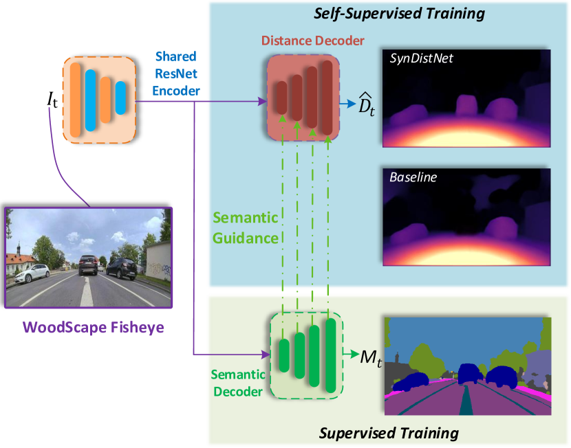
Figure 1: Overview over the joint prediction of distance $\hat{D}_{t}$ and semantic segmentation $M_{t}$ from a single input image $I_{t}$. Compared to previous approaches, our semantically guided distance estimation produces sharper depth edges and reasonable distance estimates for dynamic objects.

Depth estimation plays a vital role in 3D geometry perception of a scene in various application domains such as virtual reality and autonomous driving. As LiDAR-based depth perception is sparse and costly, image-based methods are of significant interest in perception systems regarding coverage density and redundancy. Here, current state-of-the-art approaches do rely on neural networks [16, 68], which can even be trained in an entirely self-supervised fashion from sequential images [74], giving a clear advantage in terms of applicability to arbitrary data domains over supervised approaches.

While most academic works focus on pinhole cameras [74, 18, 37, 20], many real-world applications rely on more advanced camera geometries as, e.g., fisheye camera images. There is little work on visual perception tasks on fisheye cameras [53, 63, 32, 13, 51, 54]. With this observation, in this paper, we present our proposed improvements not only on pinhole camera images but also on fisheye camera images (cf. Ravi Kumar et al. [31, 46]). We show that our self-supervised distance estimation (a generalization of depth estimation) works for both considered camera geometries. Our first contribution in that sense is the novel application of a general and robust loss function proposed by [2] to the task of self-supervised distance estimation, which replaces the de facto standard of an $L_{1}$ loss function used in previous approaches [5, 20, 22, 46, 31].

As the distance predictions are still imperfect due to the monocular cues such as occlusion, blur, haze, and different lighting conditions and the dynamic objects during the self-supervised optimizations between consecutive frames. Many approaches consider different scene understanding modalities, such as segmentation [38, 23, 45] or optical flow [65, 8] within multi-task learning to guide and improve the distance estimation. As optical flow is usually also predicted in a self-supervised fashion [35] it is therefore subject to similar limitations as the self-supervised distance estimation, which is why we focus on the joint learning of self-supervised distance estimation and semantic segmentation.

In this context, we propose a novel architecture for the joint learning of self-supervised distance estimation and semantic segmentation, which introduces a significant change compared to earlier works [23]. We first propose the novel application of self-attention layers in the ResNet encoder used for distance estimation. We also employ pixel adaptive convolutions within the decoder for robust semantic feature guidance, as proposed by [23]. However, we train the semantic segmentation simultaneously, which introduces a more favorable one-stage training than other approaches relying on pre-trained models [5, 6, 23, 38].

As depicted in Fig. 1, dynamic objects induce a lot of unfavorable artifacts and hinder the photometric loss during the training, which results in infinite distance predictions, e.g., due to their violation of the static world assumption. Therefore, we use the segmentation masks to apply a simple semantic masking technique, based on the temporal consistency of consecutive frames, which delivers significantly improved results, e.g., concerning the infinite depth problem of objects, moving at the same speed as the ego-camera. Previous approaches [36, 45, 65] did predict these motion masks only implicitly as part of the projection model and therefore were limited to the projection model’s fidelity.

Our contributions are the following: Firstly, we introduce a novel architecture for the learning of self-supervised distance estimation synergized with semantic segmentation. Secondly, we improve the self-supervised distance estimation by a general and robust loss function. Thirdly, we propose a solution for the dynamic object impact on self-supervised distance estimation by using semantic-guidance. We show the effectiveness of our approach both on pinhole and fisheye camera datasets and present state-of-the-art results for both image types.

2 Related Work

In this section, we first provide an overview of self-supervised depth/distance estimation approaches. Afterward, we discuss their combination with other tasks in multi-task learning settings and particular methods utilizing semantic guidance.

Self-Supervised Depth Estimation Garg et al. [18], and Zhou et al. [74] showed that it is possible to train networks in a self-supervised fashion by modeling depth as part of a geometric projection between stereo images and sequential images, respectively. The initial concept has been extended by considering improved loss functions [1, 19, 37, 20], the application of generative adversarial networks (GANs) [1, 12, 43] or generated proxy labels from traditional stereo algorithms [50], or synthetic data [4]. Other approaches proposed to use specialized architectures for self-supervised depth estimation [22, 57, 73], they apply teacher-student learning [42] to use test-time refinement strategies [5, 6], to employ recurrent neural networks [60, 69], or to predict the camera parameters [21] to enable training across images from different cameras.

A recent approach by Ravi Kumar et al. [31, 46] presents a successful proof of concept for the application of self-supervised depth estimation methods on the task of distance estimation from fish-eye camera images, which is used as a baseline during this work. Recent approaches also investigated the application of self-supervised depth estimation to $360^{\circ}$ images [58, 25]. However, apart from these works, the application of self-supervised depth estimation to more advanced geometries, such as fish-eye camera images, has not been investigated extensively, yet.

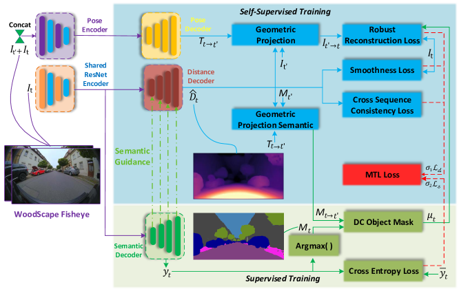
Figure 2: Overview of our proposed framework for the joint prediction of distance and semantic segmentation. The upper part (blue blocks) describes the single steps for the depth estimation, while the green blocks describe the single steps needed for the prediction of the semantic segmentation. Both tasks are optimized inside a multi-task network by using the weighted total loss described in Eq. 8.

Multi-Task Learning In contrast to letting a network predict one single task, it is also possible to train a network to predict several tasks at once, which has been shown to improve tasks such as, e.g., semantic segmentation, [29, 30, 48, 10, 11], domain adaptation [3, 40, 72], instance segmentation: [28] and depth estimation [14, 26, 59]. While initial works did weigh losses [14] or gradients [17] by an empirical factor, current approaches can estimate this scale factor automatically [26, 9]. We adopt the uncertainty-based task weighting of Kendall et al. [26].

Many recent approaches aim to integrate optical flow into the self-supervised depth estimation training, as this additional task can also be trained in a self-supervised fashion [35, 47]. In these approaches, both tasks are predicted simultaneously. Then losses are applied to enforce cross-task consistency [34, 36, 61, 65], to enforce known geometric constraints [8, 45], or to induce a modified reconstruction of the warped image [8, 66]. Although the typical approach is to compensate using optical flow, we propose an alternative method to use semantic segmentation instead for two reasons. Firstly, semantic segmentation is a mature and common task in autonomous driving, which can be leveraged. Second of all, optical flow is computationally more complex and harder to validate because of difficulties in obtaining ground truth.

Semantically-Guided Depth Estimation Several recent approaches also used semantic or instance segmentation techniques to identify moving objects and handle them accordingly inside the photometric loss [5, 6, 38, 56, 23]. To this end, the segmentation masks are either given as an additional input to the network [38, 23] or used to predict poses for each object separately between two consecutive frames [5, 6, 56] and apply a separate rigid transformation for each object. Avoiding an unfavorable two-step (pre)training procedure, other approaches in [7, 39, 64, 75] train both tasks in one multi-task network simultaneously, improving the performance by cross-task guidance between these two facets of scene understanding. Moreover, the segmentation masks can be projected between frames to enforce semantic consistency [7, 64], or the edges can be enforced to appear in similar regions in both predictions [7, 75]. In this work, we propose to use this warping to discover frames with moving objects and learn their depth from these frames by applying a simple semantic masking technique. We also propose a novel self-attention-based encoder and semantic features guidance to the decoder using pixel-adaptive convolutions as in [23]. We can apply a one-stage training by this simple change, removing the need to pretrain a semantic segmentation network.

3 Multi-Task Learning Framework

In this section, we describe our framework for the multi-task learning of distance estimation and semantic segmentation. We first state how we train the tasks individually and how they are trained in a synergized fashion.

3.1 Self-Supervised Distance Estimation Baseline

Our self-supervised depth and distance estimation is developed within a self-supervised monocular structure-from-motion (SfM) framework which requires two networks aiming at learning:

1. a monocular depth/distance model $g_{D}:I_{t}\to\hat{D}_{t}$ predicting a scale-ambiguous depth or distance (the equivalent of depth for general image geometries) $\hat{D}_{t}=g_{D}(I_{t}(ij))$ per pixel $ij$ in the target image $I_{t}$; and

2. an ego-motion predictor $g_{T}:(I_{t},I_{t^{\prime}})\to T_{t\to t^{\prime}}$ predicting a set of 6 degrees of freedom which implement a rigid transformation $T_{t\rightarrow t^{\prime}}\in\text{SE(3)}$, between the target image $I_{t}$ and the set of reference images $I_{t^{\prime}}$. Typically, $t^{\prime}\in\{t+1,t-1\}$, i.e. the frames $I_{t-1}$ and $I_{t+1}$ are used as reference images, although using a larger window is possible.

In the following part, we will describe our different loss contributions in the context of fisheye camera images.

Total Self-Supervised Objective Loss View synthesis is performed by incorporating the projection functions from FisheyeDistanceNet [31], and the same protocols are used to train the distance and pose estimation networks simultaneously. Our self-supervised objective loss consists of a reconstruction matching term $\mathcal{L}_{r}$ that is calculated between the reconstructed $\hat{I}_{t^{\prime}\to t}$ and original $I_{t}$ target images, and an inverse depth or distance regularization term $\mathcal{L}_{s}$ introduced in [19] that ensures edge-aware smoothing in the distance estimates $\hat{D}_{t}$. Finally, we apply a cross-sequence distance consistency loss $\mathcal{L}_{dc}$ derived from the chain of frames in the training sequence and the scale recovery technique from [31]. The final objective loss $\mathcal{L}_{tot}$ is averaged per pixel, scale and image batch, and is defined as:

$$\mathcal{L}_{tot}=\mathcal{L}_{r}(I_{t},\hat{I}_{t^{\prime}\to t})+\beta~{}\mathcal{L}_{s}(\hat{D}_{t})+\gamma~{}\mathcal{L}_{dc}(\hat{D}_{t},\hat{D}_{t^{\prime}})$$ (1)

where $\beta$ and $\gamma$ are weight terms between the distance regularization $\mathcal{L}_{s}$ and the cross-sequence distance consistency $\mathcal{L}_{dc}$ losses, respectively.

Image Reconstruction Loss Most state-of-the-art self-supervised depth estimation methods use heuristic loss functions. However, the optimal choice of a loss function is not well defined theoretically. In this section, we emphasize the need for exploration of a better photometric loss function and explore a more generic robust loss function.

Following previous works [31, 19, 20, 71, 22], the image reconstruction loss between the target image $I_{t}$ and the reconstructed target image $\hat{I}_{t^{\prime}\to t}$ is calculated using the $L_{1}$ pixel-wise loss term combined with Structural Similarity (SSIM) [62]

$$\tilde{\mathcal{L}}_{r}(I_{t},\hat{I}_{t^{\prime}\to t}) =\omega~{}\frac{1-\text{SSIM}(I_{t},\hat{I}_{t^{\prime}\to t})}{2}$$

$$\quad+(1-\omega)~{}\left\|(I_{t}-\hat{I}_{t^{\prime}\to t})\right\|$$ (2)

where $\omega=0.85$ is a weighting factor between both loss terms. The final per-pixel minimum reconstruction loss $\mathcal{L}_{r}$ [20] is then calculated over all the source images

$$\mathcal{L}_{r} =\min_{t^{\prime}\in\{t+1,t-1\}}\tilde{\mathcal{L}}_{r}(I_{t},\hat{I}_{t^{\prime}\to t})$$ (3)

We also incorporate the insights introduced in [20], namely auto-masking, which mitigates the impact of static pixels by removing those with unchanging appearance between frames and inverse depth map upsampling which helps to removes texture-copy artifacts and holes in low-texture regions.

3.2 Semantic Segmentation Baseline

We define semantic segmentation as the task of assigning a pixel-wise label mask $M_{t}$ to an input image $I_{t}$, i.e. the same input as for distance estimation from a single image. Each pixel gets assigned a class label $s\in\mathcal{S}=\left\{1,2,...,S\right\}$ from the set of classes $\mathcal{S}$. In a supervised way, the network predicts a posterior probability $Y_{t}$ that a pixel belongs to a class $s\in\mathcal{S}$, which is then compared to the one-hot encoded ground truth labels $\overline{Y}_{t}$ inside the cross-entropy loss

$$\mathcal{L}_{ce}=-\sum_{s\in\mathcal{S}}\overline{Y}_{t,s}\cdot\log\left(Y_{t,s}\right)$$ (4)

the final segmentation mask $M_{t}$ is then obtained by applying a pixel-wise $\operatorname{argmax}$ operation on the posterior probabilities $Y_{t,s}$. Note that we also use unrectified fisheye camera images, for which the segmentation task can however still be applied as shown in this work.

(a)

(b)

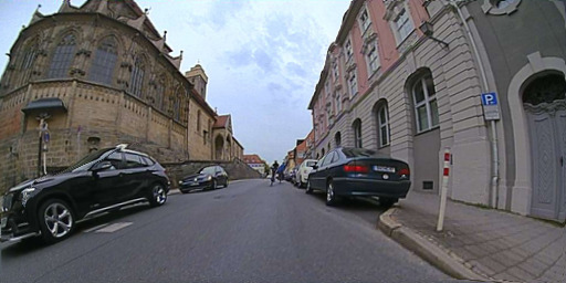
(c)

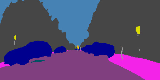
(d)

(e)

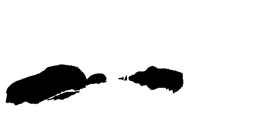
(f)

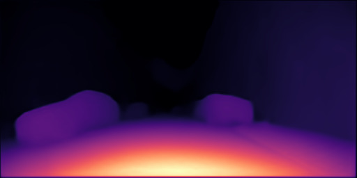
(g)

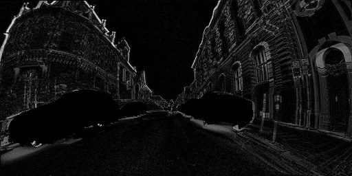
(h)

Figure 3: Application of our semantic masking methods, to handle potentially dynamic objects. The dynamic objects inside the segmentation masks from consecutive frames in (b) and (d) are accumulated to a dynamic object mask, which is used to mask the photometric error (e), as shown in (h).

3.3 Robust Reconstruction Loss for Distance Estimation

Towards developing a more robust loss function, we introduce the common notion of a per-pixel regression $\rho$ in the context of depth estimation, which is given by

$$\rho\left(\xi\right)=\rho\left(\hat{I}_{t^{\prime}\to t}-I_{t}\right)$$ (5)

while this general loss function can be implemented by a simple $L_{1}$ loss as in the second term of Eq. 3.1, recently, a general and more robust loss function is proposed by Barron [2], which we use to replace the $L_{1}$ term in Eq. 3.1. This function is a generalization of many common losses such as the $L_{1}$, $L_{2}$, Geman-McClure, Welsch/Leclerc, Cauchy/Lorentzian and Charbonnier loss functions. In this loss, robustness is introduced as a continuous parameter and it can be optimized within the loss function to improve the performance of regression tasks. This robust loss function $\rho_{\mathrm{rob}}$ is given by:

$$\rho_{\mathrm{rob}}\left(\xi\right)=\frac{\lvert\alpha-2\rvert}{\alpha}\left(\left({\frac{\left(\nicefrac{{\xi}}{{c}}\right)^{2}}{\lvert\alpha-2\rvert}}+1\right)^{\nicefrac{{\alpha}}{{2}}}-1\right)$$ (6)

The free parameters $\alpha$, and $c$ in this loss can be automatically adapted to the particular problem via a data-driven optimization, as described in [2].

3.4 Dealing With Dynamic Objects

Typically, the assumed static world model for projections between image frames is violated by the appearance of dynamic objects. Thereby, we use the segmentation masks to exclude moving potentially dynamic objects while non-moving dynamic object should still contribute.

In order to implement this, we aim at defining a pixel-wise mask $\mu_{t}$, which contains a $0$, if a pixel belongs to a dynamic object from the current frame $I_{t}$, or to a wrongfully projected dynamic object from the reconstructed frames $\hat{I}_{t^{\prime}\to t}$, and a $1$ otherwise. For calculation of the mask, we start by predicting a semantic segmentation mask $M_{t}$ which corresponds to image $I_{t}$ and also segmentation masks $M_{t^{\prime}}$ for all images $I_{t^{\prime}}$. Then we use the same projections as for the images and warp the segmentation masks (using nearest neighbour instead of bilinear sampling), yielding projected segmentation masks $M_{t^{\prime}\to t}$. Then, also defining the set of dynamic object classes $\mathcal{S}_{\mathrm{DC}}\subset\mathcal{S}$ we can define $\mu_{t}$ by its pixel-wise elements at pixel location $ij$:

$$\!\!\mu_{t,ij}=\!\left\{\begin{array}[]{l}1,\;M_{t,ij}\notin\mathcal{S}_{\mathrm{DC}}\;\land\;M_{t^{\prime}\rightarrow t,ij}\notin\mathcal{S}_{\mathrm{DC}}\\ 0,\;\mathrm{else}\\ \end{array}\right.$$ (7)

The mask is then applied pixel-wise on the reconstruction loss defined in Eq. 3.1, in order to mask out dynamic objects. However, as we only want to mask out moving DC-objects, we detect them using the consistency of the target segmentation mask and the projected segmentation mask to judge whether dynamic objects are moving between consecutive frames (e.g., we intend to learn the depth of dynamic objects from parking cars, but not from driving ones). With this measure, we apply the dynamic object mask $\mu_{t}$ only to an imposed fraction $\epsilon$ of images, in which the objects are detected as mostly moving.

3.5 Joint Optimization

We incorporate the task weighting approach by Kendall et al. [26]; we weigh our distance estimation and semantic segmentation loss terms for multi-task learning, which enforces homoscedastic (task) uncertainty. It is proven to be effective in weighing the losses from Eq. 1 and Eq. 4 by:

$$\frac{1}{2\sigma_{1}^{2}}\mathcal{L}_{tot}+\frac{1}{2\sigma_{2}^{2}}\mathcal{L}_{ce}+\log(1+\sigma_{1})+\log(1+\sigma_{2})$$ (8)

Homoscedastic uncertainty does not change with varying input data and is task-specific. We, therefore, learn this uncertainty and use it to down weigh each task. Increasing the noise parameter $\sigma$ reduces the weight for the respective task. Furthermore, $\sigma$ is a learnable parameter; the objective optimizes a more substantial uncertainty that should lead to a smaller contribution of the task’s loss to the total loss. In this case, the different scales from the distance and semantic segmentation are weighed accordingly. The noise parameter $\sigma_{1}$ tied to distance estimation is quite low compared to $\sigma_{2}$ of semantic segmentation, and the convergence occurs accordingly. Higher homoscedastic uncertainty leads to a lower impact of the task’s network weight update. It is important to note that this technique is not limited to the joint learning of distance estimation and semantic segmentation, but can also be applied to more tasks and arbitrary camera geometries.

4 Network Architecture

In this section, we will describe our novel architecture for self-supervised distance estimation utilizing semantic guidance. The baseline from [31] used deformable convolutions to model the fisheye geometry to incorporate the distortion and improve the distance estimation accuracy. In this work, we introduce a self-attention based encoder to handle the view synthesis and a semantically guided decoder, which can be trained in a one-stage fashion.

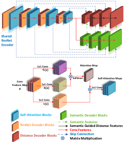
Figure 4: Visualization of our proposed network architecture to semantically guide the depth estimation. We utilize a self-attention based encoder and a semantically guided decoder using pixel-adaptive convolutions.

4.1 Self-Attention Encoder

Previous depth estimation networks [20, 74] use normal convolutions for capturing the local information in an image, but the convolutions’ receptive field is relatively small. Inspired by [44], who took self-attention in CNNs even further by using stand-alone self-attention blocks instead of only enhancing convolutional layers. The authors present a self-attention layer which may replace convolution while reducing the number of parameters. Similar to a convolution, given a pixel $x_{ij}\in\mathbb{R}^{d_{in}}$ inside a feature map, the local region of pixels defined by positions ${ab}\in\mathcal{N}_{k}(ij)$ with spatial extent $k$ centered around $x_{ij}$ are extracted initially which is referred to as a memory block. For every memory block, the single-headed attention for computing the pixel output $z_{ij}\in\mathbb{R}^{d_{out}}$ is then calculated by:

$$z_{ij}=\sum_{\mathclap{ab\in\,\mathcal{N}_{k}(ij)}}\texttt{softmax}_{ab}\left(q_{ij}^{\top}k_{ab}\right)v_{ab}$$ (9)

where $q_{ij}=W_{Q}x_{ij}$ are the queries, keys $k_{ab}=W_{K}x_{ab}$, and values $v_{ab}=W_{V}x_{ab}$ are linear transformations of the pixel in position $ij$ and the neighborhood pixels. The learned transformations are denoted by the matrices W. $\texttt{softmax}_{ab}$ defines a softmax applied to all logits computed in the neighborhood of $ij$. $W_{Q},W_{K},W_{V}\in\mathbb{R}^{d_{out}\times d_{in}}$ are trainable transformation weights. There exists an issue in the above-discussed approach, as there is no positional information encoded in the attention block. Thus the Eq. 9 is invariant to permutations of the individual pixels. For perception tasks, it is typically helpful to consider spatial information in the pixel domain. For example, the detection of a pedestrian is composed of spotting faces and legs in a proper relative localization. The main advantage of using self-attention layers in the encoder is that it induces a synergy between geometric and semantic features for distance estimation and semantic segmentation tasks. In [55] sinusoidal embeddings are used to produce the absolute positional information. Following [44], instead of attention with 2D relative position embeddings, we incorporate relative attention due to their better accuracy for computer vision tasks. The relative distances of the position $ij$ to every neighborhood pixel $(a,b)$ is calculated to obtain the relative embeddings. The calculated distances are split up into row and column distances $r_{a-i}$ and $r_{b-j}$ and the embeddings are concatenated to form $r_{a-i,b-j}$ and multiplied by the query $q_{ij}$ given by:

$$z_{ij}=\sum_{\mathclap{ab\in\,\mathcal{N}_{k}(ij)}}\texttt{softmax}_{ab}\left(q_{ij}^{\top}k_{ab}+q_{ij}^{\top}r_{a-i,b-j}\right)v_{ab}$$ (10)

It ensures the weights calculated by the softmax function are modulated by both the relative distance and content of the key from the query. Instead of focusing on the whole feature map, the attention layer only focuses on the memory block.

4.2 Semantically-Guided Distance Decoder

To address the limitations of regular convolutions, we follow the approaches of [49, 23] in using pixel-adaptive convolutions for semantic guidance inside the distance estimation branch of the multi-task network. By this approach, we can break up the translation invariance of convolutions and incorporate spatially-specific information of the semantic segmentation branch.

To this end, as shown in Figure 4 we extract feature maps at different levels from the semantic segmentation branch of the multi-task network. These semantic feature maps are consequently used to guide the respective pixel-adaptive convolutional layer, following the formulation proposed in [49] to process an input signal $x$ to be convolved:

$$x_{ij}^{\prime}=\sum_{ab\in\mathcal{N}_{k}(i,j)}K(F_{ij},F_{ab})W[r_{a-i,b-j}]x_{ab}+B$$ (11)

where $\mathcal{N}_{k}(i,j)$ defines a $k\times k$ neighbourhood window around the pixel location $ij$ (distance $r_{a-i,b-j}$ between pixel locations), which is used as input to the convolution with weights $W$ (kernel size $k$), bias $B\in\mathbb{R}^{1}$ and kernel $K$, that is used in this case to calculate the correlation between the semantic guidance features $F\in\mathbb{R}^{D}$ from the segmentation network. We follow [23] in using a Gaussian kernel:

$$K(F_{ij},F_{ab})=\exp\left(-\frac{1}{2}(F_{ij}-F_{ab})^{T}\Sigma_{ijab}^{-1}(F_{ij}-F_{ab})\right)$$ (12)

with covariance matrix $\Sigma_{ijab}$ between features $F_{ij}$ and $F_{ab}$, which is chosen as a diagonal matrix $\sigma^{2}\cdot\mathbf{1}^{D}$, where $\sigma$ represents a learnable parameter for each convolutional filter.

In this work, we use pixel-adaptive convolutions to produce semantic-aware distance features, where the fixed information encoded in the semantic network is used to disambiguate geometric representations for the generation of multi-level depth features. Compared to previous approaches [5, 23], we use features from our semantic segmentation branch that is trained simultaneously with the distance estimation branch introducing a more favorable one-stage training.

5 Experimental Evaluation

Model [HTML]00b050 Segmentation (mIOU) [HTML]00b0f0 Distance (RMSE) Segmentation only baseline 76.8 ✗ Distance only baseline ✗ 2.316 MTL baseline 78.3 2.128 MTL with synergy (SynDistNet) 81.5 1.714

Table 1: Multi-task learning (MTL) ablation results on the WoodScape dataset using a ResNet18 encoder.

Network	RL	Self-Attn	SEM	Mask	[HTML]5880abLower is Better				[HTML]e8715bHigher is Better
					[HTML]5880abAbs Rel	[HTML]5880abSq Rel	[HTML]5880abRMSE	[HTML]5880abRMSElog	[HTML]e8715b$\delta<1.25$	[HTML]e8715b$\delta<1.25^{2}$	[HTML]e8715b$\delta<1.25^{3}$
FisheyeDistanceNet [31]	✗	✗	✗	✗	0.152	0.768	2.723	0.210	0.812	0.954	0.974
SynDistNet (ResNet-18)	✓	✗	✗	✗	0.142	0.537	2.316	0.179	0.878	0.971	0.985
	✓	✗	✗	✓	0.133	0.491	2.264	0.168	0.868	0.976	0.988
	✓	✓	✗	✓	0.121	0.429	2.128	0.155	0.875	0.980	0.990
	✓	✓	✓	✗	0.105	0.396	1.976	0.143	0.878	0.982	0.992
	✓	✓	✓	✓	0.076	0.368	1.714	0.127	0.891	0.988	0.994
SynDistNet (ResNet-50)	✓	✗	✗	✗	0.138	0.540	2.279	0.177	0.880	0.973	0.986
	✓	✗	✗	✓	0.127	0.485	2.204	0.166	0.881	0.975	0.989
	✓	✓	✗	✓	0.115	0.413	2.028	0.148	0.876	0.983	0.992
	✓	✓	✓	✗	0.102	0.387	1.856	0.135	0.884	0.985	0.994
	✓	✓	✓	✓	0.068	0.352	1.668	0.121	0.895	0.990	0.996

Table 2: Ablative analysis showing the effect of each of our contributions using the Fisheye WoodScape dataset [67]. The input resolution is $512\times 256$ pixels and distances are capped at $40\,m$. We start with FisheyeDistanceNet [31] baseline and incrementally add robust loss (RL), self-attention based encoder (Self-Attn), semantically-guided decoder (SEM) and dynamic object masking (Mask).

Method	[HTML]5880abAbs Rel	[HTML]5880abSq Rel	[HTML]5880abRMSE	[HTML]5880abRMSElog	[HTML]e8715b$\delta<1.25$	[HTML]e8715b$\delta<1.25^{2}$	[HTML]e8715b$\delta<1.25^{3}$
FisheyeDistanceNet [31]	0.152	0.768	2.723	0.210	0.812	0.954	0.974
SynDistNet fixed $\alpha=1$	0.148	0.642	2.615	0.203	0.824	0.960	0.978
SynDistNet fixed $\alpha=0$	0.151	0.638	2.601	0.205	0.822	0.962	0.981
SynDistNet fixed $\alpha=2$	0.154	0.631	2.532	0.198	0.832	0.965	0.981
SynDistNet adaptive $\alpha\in(0,2)$	0.142	0.537	2.316	0.179	0.878	0.971	0.985

Table 3: Ablation study on different variants of our SynDistNet using the Fisheye WoodScape dataset [67]. We replace the $L_{1}$ loss with several variants of the general loss function varying the parameter $\alpha$ and observe a significant performance improvement.

Table 1 captures the primary goal of this paper, which is to develop a synergistic multi-task network for semantic segmentation and distance estimation tasks. ResNet18 encoder was used in these experiments on the Fisheye WoodScape dataset. Firstly, we formulate single-task baselines for these tasks and build an essential shared encoder multi-task learning (MTL) baseline. The MTL results are slightly better than their respective single-task benchmarks demonstrating that shared encoder features can be learned for diverse tasks wherein segmentation captures semantic features, and distance estimation captures geometric features. The proposed synergized MTL network SynDistNet reduces distance RMSE by $25\%$ and improves segmentation accuracy by $4\%$. We break down these results further using extensive ablation experiments.

Ablation Experiments For our ablation analysis, we consider two variants of ResNet encoder heads. Distance estimation results of these variants are shown in Table 2. Significant improvements in accuracy are obtained with the replacement of $L_{1}$ loss with a generic parameterized loss function. The impact of the mask is incremental in the WoodScape dataset. Still, it poses the potential to solve the infinite depth/distance issue and provides a way to improve the photometric loss. We can see with the addition of our proposed self-attention based encoder coupled with semantic-guidance decoder architecture can consistently improve the performance. Finally, with all our additions we outperform FisheyeDistanceNet [31] for all considered metrics.

	Method	Resolution	[HTML]5880abAbs Rel	[HTML]5880abSq Rel	[HTML]5880abRMSE	[HTML]5880abRMSElog	[HTML]e8715b$\delta<1.25$	[HTML]e8715b$\delta<1.25^{2}$	[HTML]e8715b$\delta<1.25^{3}$
			[HTML]5880ablower is better				[HTML]e8715bhigher is better
[HTML]448BE9KITTI
Original [15]	EPC++ [36]	640 x 192	0.141	1.029	5.350	0.216	0.816	0.941	0.976
	Monodepth2 [20]	640 x 192	0.115	0.903	4.863	0.193	0.877	0.959	0.981
	PackNet-SfM [22]	640 x 192	0.111	0.829	4.788	0.199	0.864	0.954	0.980
	FisheyeDistanceNet [31]	640 x 192	0.117	0.867	4.739	0.190	0.869	0.960	0.982
	UnRectDepthNet [46]	640 x 192	0.107	0.721	4.564	0.178	0.894	0.971	0.986
	SynDistNet	640 x 192	0.109	0.718	4.516	0.180	0.896	0.973	0.986
	Monodepth2 [20]	1024 x 320	0.115	0.882	4.701	0.190	0.879	0.961	0.982
	FisheyeDistanceNet [31]	1024 x 320	0.109	0.788	4.669	0.185	0.889	0.964	0.982
	UnRectDepthNet [46]	1024 x 320	0.103	0.705	4.386	0.164	0.897	0.980	0.989
	SynDistNet	1024 x 320	0.102	0.701	4.347	0.166	0.901	0.980	0.990
Improved [52]	SfMLeaner [74]	416 x 128	0.176	1.532	6.129	0.244	0.758	0.921	0.971
	Vid2Depth [37]	416 x 128	0.134	0.983	5.501	0.203	0.827	0.944	0.981
	DDVO [57]	416 x 128	0.126	0.866	4.932	0.185	0.851	0.958	0.986
	EPC++ [36]	640 x 192	0.120	0.789	4.755	0.177	0.856	0.961	0.987
	Monodepth2 [20]	640 x 192	0.090	0.545	3.942	0.137	0.914	0.983	0.995
	PackNet-SfM [22]	640 x 192	0.078	0.420	3.485	0.121	0.931	0.986	0.996
	UnRectDepthNet [46]	640 x 192	0.081	0.414	3.412	0.117	0.926	0.987	0.996
	SynDistNet	640 x 192	0.076	0.412	3.406	0.115	0.931	0.988	0.996

Table 4: Quantitative performance comparison of our network with other self-supervised monocular methods for depths up to 80 m for KITTI. Original uses raw depth maps as proposed by [15] for evaluation, and Improved uses annotated depth maps from [52]. At test-time, all methods excluding FisheyeDistanceNet, PackNet-SfM and Ours, scale the estimated depths using median ground-truth LiDAR depth.

Raw Input
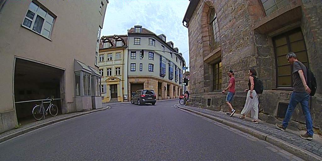
Baseline
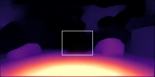
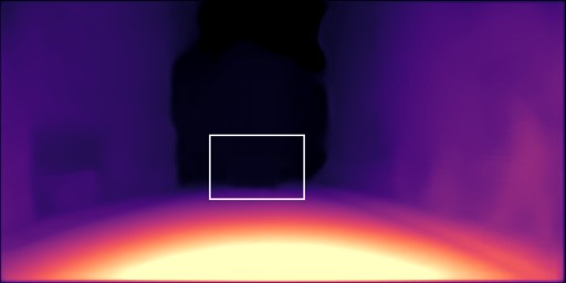
SynDistNet

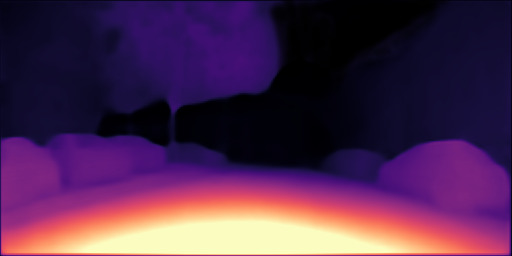
Figure 5: Qualitative result comparison on the Fisheye WoodScape dataset between the baseline model without our contributions and the proposed SynDistNet. Our SynDistNet can recover the distance of dynamic objects (left images) which eventually solves the infinite distance issue. In the 3rd and 4th columns, we can see that semantic guidance helps us to recover the thin structure and resolve the distance of homogeneous areas outputting sharp distance maps on raw fisheye images.

Robust loss function strategy We showcase that adaptive or annealed variants of the robust loss can significantly improve the performance. Compared to [2] we retained the edge smoothness loss from FisheyeDistanceNet [31] as it yielded better results. The fixed scale assumption is matched by setting the loss’s scale $c$ fixed to $0.01$, which also roughly matches the shape of its $L_{1}$ loss. For the fixed scale models in Table 3, we used a constant value for $\alpha$. In the adaptive $\alpha\in(0,2)$ variant, $\alpha$ is made a free parameter and is allowed to be optimized along with the network weights during training. The adaptive plan of action outperforms the fixed strategies, which showcases the importance of allowing the model to regulate the robustness of its loss during training adaptively.

KITTI Evaluation As there is little work on fisheye distance estimation, we evaluate our method on extensively used KITTI dataset using the metrics proposed by Eigen et al. [15] to facilitate comparison. The quantitative results are shown in the Table 4 illustrate that the improved scale-aware self-supervised approach outperforms all the state-of-the-art monocular approaches. More specifically, we improve the baseline FisheyeDistanceNet with the usage of a general and adaptive loss function [2] which is showcased in Table 3 and better architecture. We could not leverage the Cityscapes dataset into our training regime to benchmark our scale-aware framework due to the absence of odometry data. Compared to PackNet-SfM [22], which presumably uses a superior architecture than our ResNet18, where they estimate scale-aware depths with their velocity supervision loss using the ground truth poses for supervision. We only rely on speed and time data captured from the vehicle odometry, which is easier to obtain. Our approach can be easily transferred to the domain of aerial robotics as well. We could achieve higher accuracy than PackNet, which can be seen in Table 4.

6 Conclusion

Geometry and appearance are two crucial cues of scene understanding, e.g., in automotive scenes. In this work, we develop a multi-task learning model to estimate metric distance and semantic segmentation in a synergized manner. Specifically, we leverage the semantic segmentation of potentially moving objects to remove wrongful projected objects inside the view synthesis step. We also propose a novel architecture to semantically guide the distance estimation that is trainable in a one-stage fashion and introduce the application of a robust loss function. Our primary focus is to develop our proposed model for less explored fisheye cameras based on the WoodScape dataset. We demonstrate the effect of each proposed contribution individually and obtain state-of-the-art results on both WoodScape and KITTI datasets for self-supervised distance estimation.

Supplementary Material

1 Additional Method Details

Edge-Aware Distance Smoothness Loss: In order to regularize distance and avoid divergent values in occluded or texture-less low-image gradient areas, we add a geometric smoothing loss. We adopt the edge-aware term similar to [20]. The regularization term is imposed on the inverse distance map. The loss is weighted for each of the image pyramid levels and is decayed by a factor of 2 on each downsampling.

$$\mathcal{L}_{s}(\hat{D}_{t})=|\partial_{u}\hat{D}^{*}_{t}|e^{-|\partial_{u}I_{t}|}+|\partial_{v}\hat{D}^{*}_{t}|e^{-|\partial_{v}I_{t}|}$$ (13)

To discourage shrinking of distance estimates [57], mean-normalized inverse distance of $D_{t}$ is considered, i.e. $\hat{D}^{*}_{t}=\hat{D}^{-1}_{t}/\overline{D}_{t}$, where $\overline{D}_{t}$ denotes the mean of $\hat{D}^{-1}_{t}:=1/\hat{D}_{t}$.

Cross-Sequence Distance Consistency Loss: Following FisheyeDistanceNet [31], we enforce the cross-sequence distance consistency loss (CSDCL) for the training sequence $S$:

$$\mathcal{L}_{dc}=\sum_{t=1}^{N-1}\sum_{t^{\prime}=t+1}^{N}\bigg{(} \sum_{p_{t}}\left|D_{t\to t^{\prime}}\left(p_{t}\right)-\hat{D}_{t\to t^{\prime}}\left(p_{t}\right)\right|$$

$$+ \sum_{p_{t^{\prime}}}\left|D_{t^{\prime}\to t}\left(p_{t^{\prime}}\right)-\hat{D}_{t^{\prime}\to t}\left(p_{t^{\prime}}\right)\right|\bigg{)}$$ (14)

Eq. 1 contains one term for which pixels and point clouds are warped forwards in time (from $t$ to $t^{\prime}$) and one term for which they are warped backwards in time (from $t^{\prime}$ to $t$), where $\hat{D}_{t^{\prime}}$ and $\hat{D}_{t}$ are the estimates of the images $I_{t^{\prime}}$ and $I_{t}$ respectively for each pixel ${{p}_{t}}\in{{I}_{t}}$.

Raw Input
Baseline
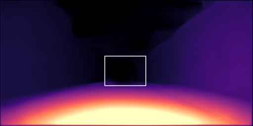
SynDistNet
SynDistNet

Figure 6: Qualitative result comparison on the Fisheye WoodScape dataset between the baseline model without our contributions and the proposed SynDistNet. Our SynDistNet can recover the distance of dynamic objects (left images) which eventually solves the infinite distance issue. In the 3rd and 4th columns, we can see that semantic guidance helps us to obtain curbs and resolve the distance of homogeneous areas outputting sharp distance maps on raw fisheye images. The final row indicates the semantic segmentation predictions.

Additional Considerations: In all the previous works [74, 20, 22], networks are trained to recover inverse depth $g_{d}:p\mapsto g^{-1}_{D}(I_{t}(p))$. A limitation of these approaches is that both depth or distance and pose are estimated up to an unknown scale factor. We incorporate the scale recovery technique from FisheyeDistanceNet [31] and obtain scale-aware depth and distance directly for pinhole and fisheye images. We also incorporate the clipping of the photometric loss values, which improves the optimization process and provides a way to strengthen the photometric error. Additionally, we include the backward sequence training regime, which helps to resolve the unknown distance estimates in the image border.

2 Implementation Details

Raw Input	Zhou [74]	Godard [20]	SynDistNet

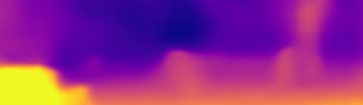
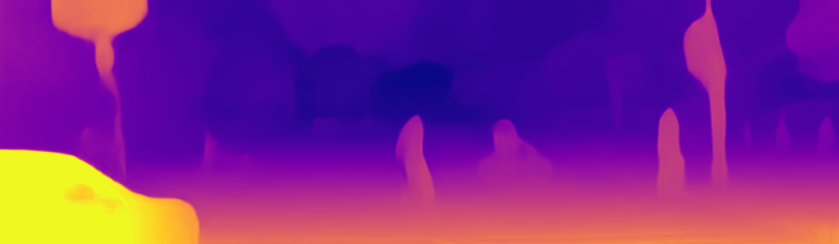
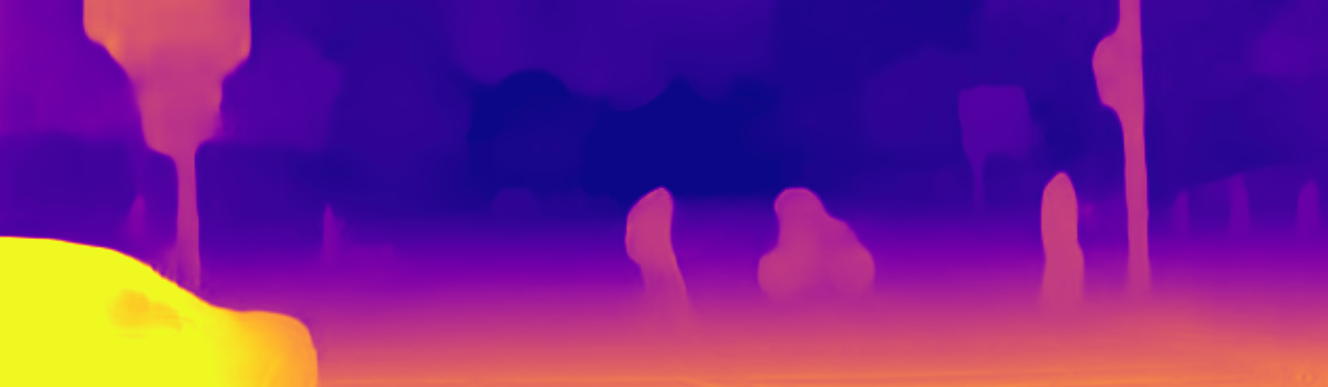
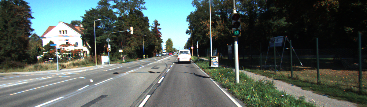
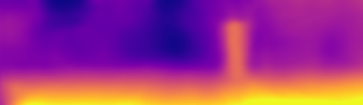
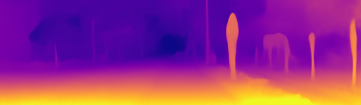
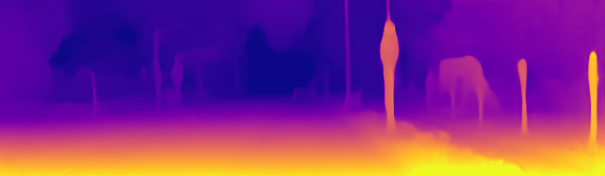
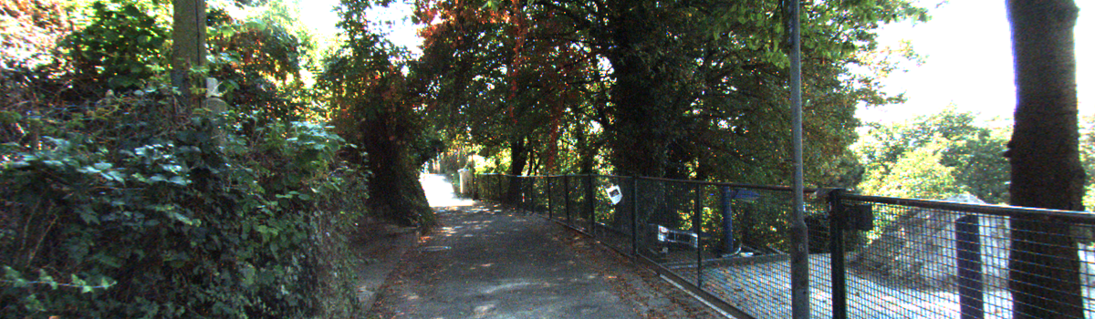
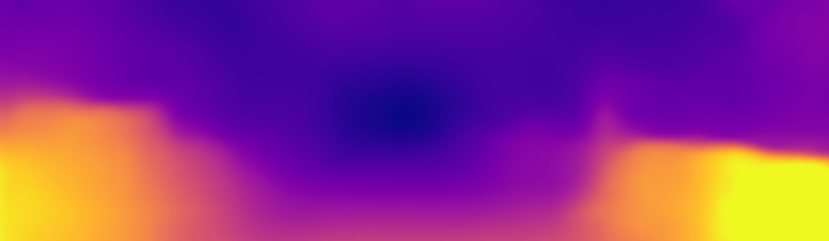
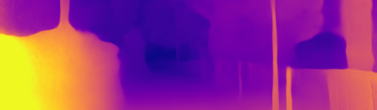
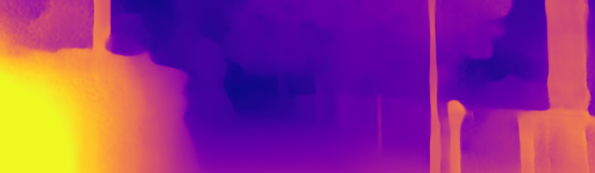
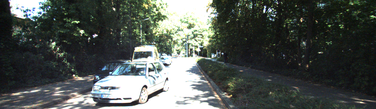
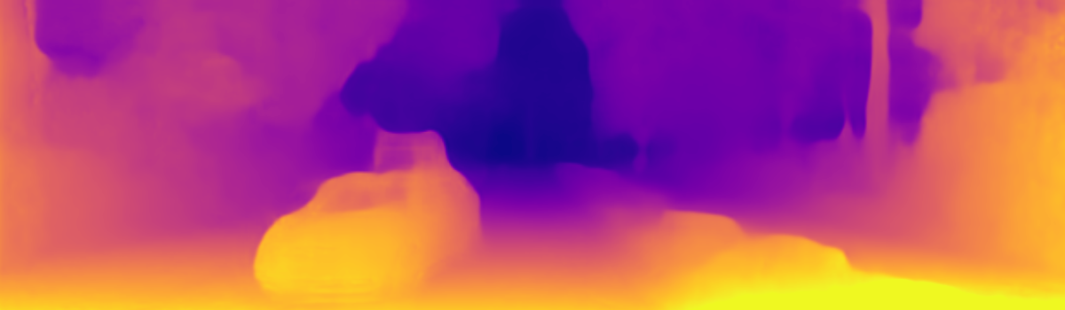
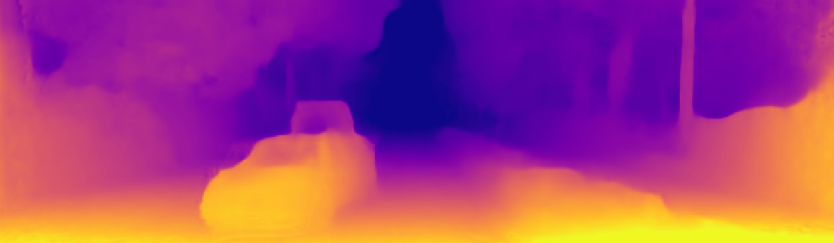
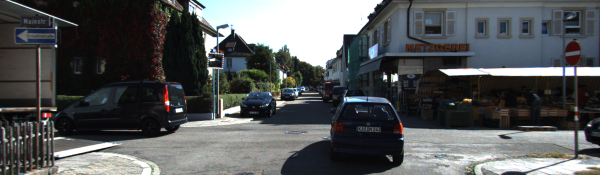
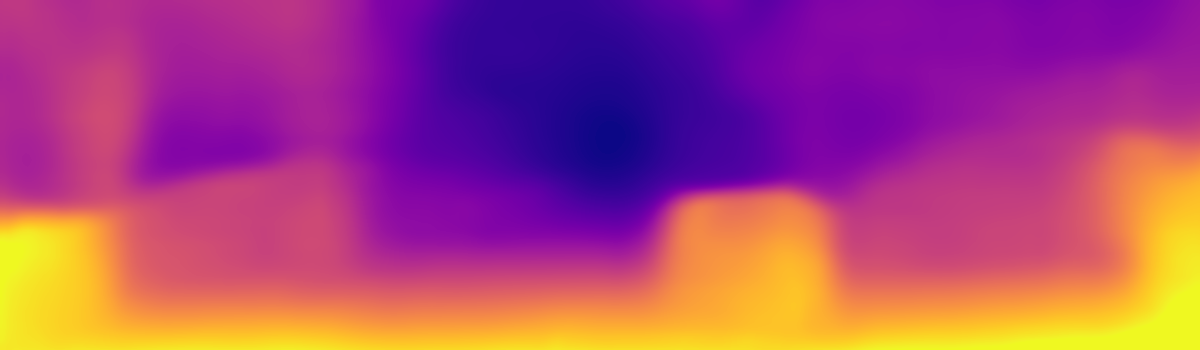
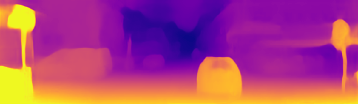
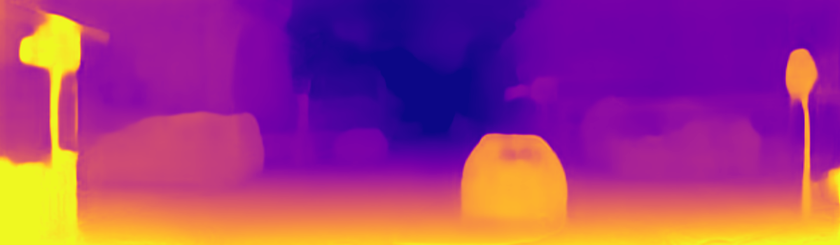
Figure 7: Qualitative results on the KITTI dataset. Our SynDistNet produces sharp depth maps on raw pinhole camera images and can recover the distance of dynamic objects.

Raw Input
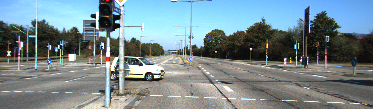
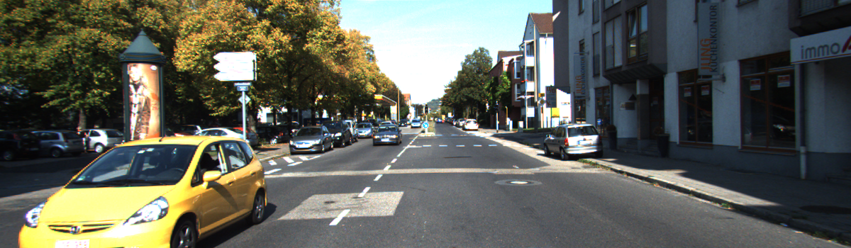
SynDistNet
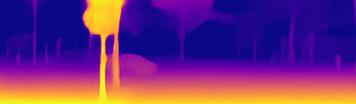
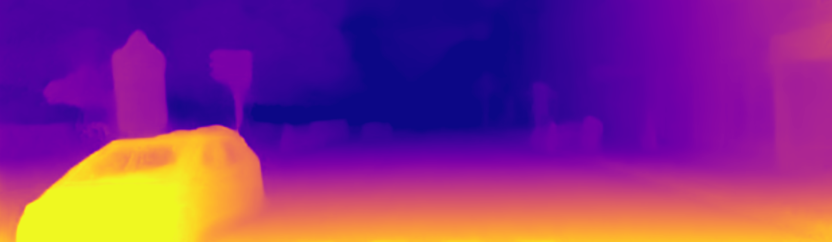
SynDistNet
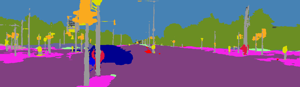
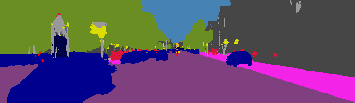
Raw Input
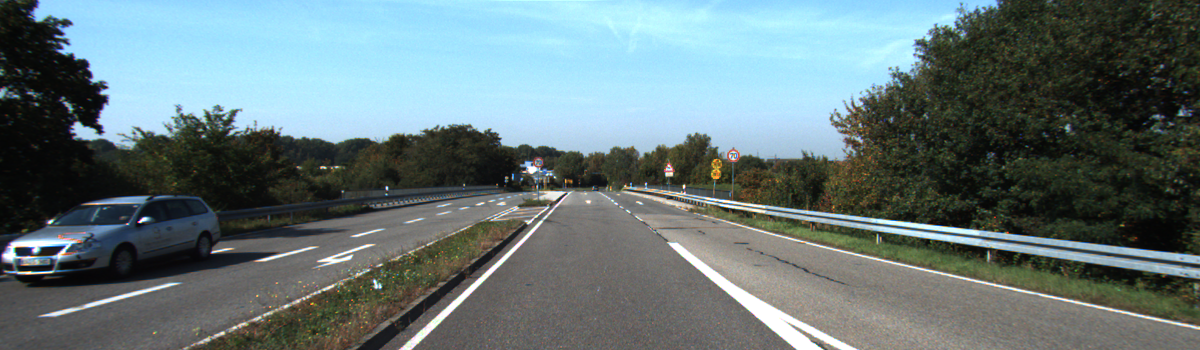
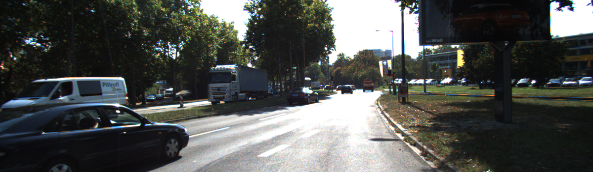
SynDistNet
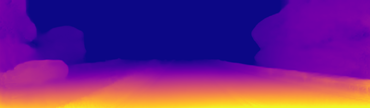
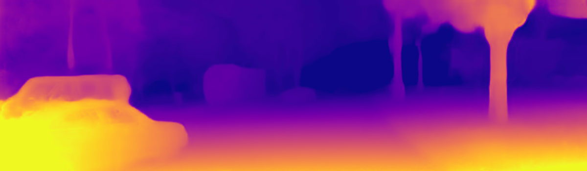
SynDistNet

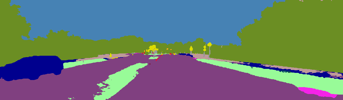
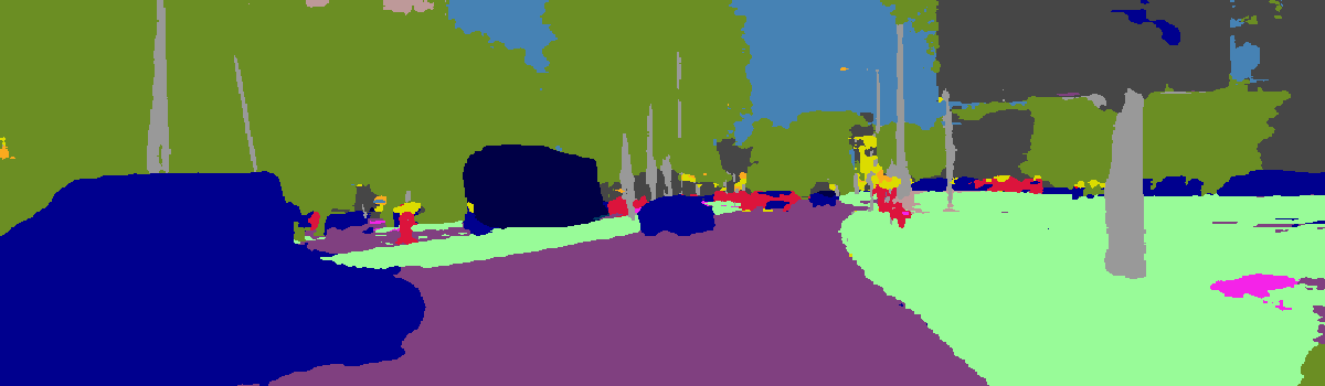
Figure 8: Qualitative results on the KITTI dataset. We showcase depth estimation as well as semantic segmentation outputs on the KITTI dataset using our SynDistNet.

The distance estimation network is mainly based on FisheyeDistanceNet [31], an encoder-decoder network with skip connections. After testing different variants of ResNet family, we chose ResNet18 [24] as the encoder as it provides a high-quality distance prediction, and improvements in higher complexity encoders were incremental. It would also aid in obtaining real-time performance on low-power embedded systems. We also incorporate self-attention layers in the encoder and drop the deformable convolutions used in the baseline model. We could leverage the usage of a more robust loss function over $L_{1}$ to reduce training times on ResNet18 by performing a single-scale image depth prediction than the multi-scale in [31]. The semantic segmentation is trained in a supervised fashion with Cross-Entropy loss and is jointly optimised along with the distance estimation. We use Pytorch [41] and employ Ranger (RAdam [33] + LookAhead [70]) optimizer to minimize the training objective function than the previously employed Adam [27]. RAdam leverages a dynamic rectifier to adjust Adam’s adaptive momentum based on the variance and effectively provides an automated warm-up custom-tailored to the current dataset to ensure a solid start to training. LookAhead ”lessens the need for extensive hyperparameter tuning” while achieving ”faster convergence across different deep learning tasks with minimal computational overhead.” Hence, both provide breakthroughs in different aspects of deep learning optimization, and the combination is highly synergistic, possibly providing the best of both improvements for the results.

We train the model for 17 epochs, with a batch size of 20 on 24GB Titan RTX with an initial learning rate of ${{10}^{-4}}$ for the first 12 epochs, then drop to ${{10}^{-5}}$ for the last 5 epochs. A significant decrease in training time of 8 epochs over the previous training of the model for 25 epochs in FisheyeDistanceNet [31]. The sigmoid output $\sigma$ from the distance decoder is converted to distance with $D={a\cdot\sigma+b}$. For the pinhole model, depth $D=1/({a\cdot\sigma+b})$, where $a$ and $b$ are chosen to constrain $D$ between $0.1$ and $100$ units. The original input resolution of the fisheye image is $1280\times 800$ pixels; we crop it to $1024\times 512$ to remove the vehicle’s bumper, shadow, and other artifacts of the vehicle. Finally, the cropped image is downscaled to $512\times 256$ before feeding to the network. For the pinhole model on KITTI, we use $640\times 192$ pixels as the network input.

3 Qualitative Results

Figure 6 and Figure 8 provides qualitative results of SynDistNet on WoodScape and KITTI test dataset for segmentation and depth estimation tasks respectively. Figure 7 illustrates the qualitative comparison of depth estimation with the recent state of the art methods.

References

- [1] Filippo Aleotti, Fabio Tosi, Matteo Poggi, and Stefano Mattoccia. Generative Adversarial Networks for Unsupervised Monocular Depth Prediction. In Proc. of ECCV - Workshops, 2018.
- [2] Jonathan T. Barron. A General and Adaptive Robust Loss Function. In Proc. of CVPR, 2019.
- [3] Jan-Aike Bolte, Markus Kamp, Antonia Breuer, Silviu Homoceanu, Peter Schlicht, Fabian Huger, Daniel Lipinski, and Tim Fingscheidt. Unsupervised Domain Adaptation to Improve Image Segmentation Quality Both in the Source and Target Domain. In Proc. of CVPR - Workshops, 2019.
- [4] Behzad Bozorgtabar, Mohammad Saeed Rad, Dwarikanath Mahapatra, and Jean-Philippe Thiran. SynDeMo: Synergistic Deep Feature Alignment for Joint Learning of Depth and Ego-Motion. In Proc. of ICCV, 2019.
- [5] Vincent Casser, Soeren Pirk, Reza Mahjourian, and Anelia Angelova. Depth Prediction Without the Sensors: Leveraging Structure for Unsupervised Learning from Monocular Videos. In Proc. of AAAI, 2019.
- [6] Vincent Casser, Soeren Pirk, Reza Mahjourian, and Anelia Angelova. Unsupervised Monocular Depth and Ego-Motion Learning With Structure and Semantics. In Proc. of CVPR - Workshops, 2019.
- [7] Po-Yi Chen, Alexander H. Liu, Yen-Cheng Liu, and Yu-Chiang F. Wang. Towards Scene Understanding: Unsupervised Monocular Depth Estimation With Semantic-Aware Representation. In Proc. of CVPR, 2019.
- [8] Yuhua Chen, Cordelia Schmid, and Cristian Sminchisescu. Self-Supervised Learning With Geometric Constraints in Monocular Video Connecting Flow, Depth, and Camera. In Proc. of ICCV, 2019.
- [9] Zhao Chen, Vijay Badrinarayanan, Chen-Yu Lee, and Andrew Rabinovich. GradNorm: Gradient Normalization for Adaptive Loss Balancing in Deep Multitask Networks. In Proc. of ICML, 2018.
- [10] Sumanth Chennupati, Ganesh Sistu, Senthil Yogamani, and Samir A Rawashdeh. Multinet++: Multi-stream feature aggregation and geometric loss strategy for multi-task learning. In Proceedings of the IEEE Conference on Computer Vision and Pattern Recognition Workshops, 2019.
- [11] Sumanth Chennupati, Ganesh Sistu, Senthil Yogamani, and Samir Rawashdeh. Auxnet: Auxiliary tasks enhanced semantic segmentation for automated driving. In Proceedings of the 14th International Joint Conference on Computer Vision, Imaging and Computer Graphics Theory and Applications (VISAPP), 2019.
- [12] Arun CS Kumar, Suchendra M. Bhandarkar, and Mukta Prasad. Monocular Depth Prediction Using Generative Adversarial Networks. In Proc. of CVPR - Workshops, 2018.
- [13] Ashok Dahal, Jakir Hossen, Chennupati Sumanth, Ganesh Sistu, Kazumi Malhan, Muhammad Amasha, and Senthil Yogamani. Deeptrailerassist: Deep learning based trailer detection, tracking and articulation angle estimation on automotive rear-view camera. In Proceedings of the IEEE International Conference on Computer Vision Workshops, 2019.
- [14] David Eigen and Rob Fergus. Predicting Depth, Surface Normals and Semantic Labels With a Common Multi-Scale Convolutional Architecture. In Proc. of ICCV, 2015.
- [15] David Eigen, Christian Puhrsch, and Rob Fergus. Depth Map Prediction from a Single Image Using a Multi-Scale Deep Network. In Proc. of NIPS, 2014.
- [16] Huan Fu, Mingming Gong, Chaohui Wang, Kayhan Batmanghelich, and Dacheng Tao. Deep Ordinal Regression Network for Monocular Depth Estimation. In Proc. of CVPR, 2018.
- [17] Yaroslav Ganin and Victor Lempitsky. Unsupervised Domain Adaptation by Backpropagation. In Proc. of ICML, 2015.
- [18] Ravi Garg, Vijay Kumar BG, Gustavo Carneiro, and Ian Reid. Unsupervised CNN for Single View Depth Estimation: Geometry to the Rescue. In Proc. of ECCV, 2016.
- [19] Clément Godard, Oisin Mac Aodha, and Gabriel J. Brostow. Unsupervised Monocular Depth Estimation With Left-Right Consistency. In Proc. of CVPR, 2017.
- [20] Clément Godard, Oisin Mac Aodha, Michael Firman, and Gabriel J. Brostow. Digging Into Self-Supervised Monocular Depth Estimation. In Proc. of ICCV, 2019.
- [21] Ariel Gordon, Hanhan Li, Rico Jonschkowski, and Anelia Angelova. Depth from Videos in the Wild: Unsupervised Monocular Depth Learning from Unknown Cameras. In Proc. of ICCV, 2019.
- [22] Vitor Guizilini, Rares Ambrus, Sudeep Pillai, and Adrien Gaidon. 3D Packing for Self-Supervised Monocular Depth Estimation. In Proc. of CVPR, 2020.
- [23] Vitor Guizilini, Rui Hou, Jie Li, Rares Ambrus, and Adrien Gaidon. Semantically-Guided Representation Learning for Self-Supervised Monocular Depth. In Proc. of ICLR, 2020.
- [24] Kaiming He, Xiangyu Zhang, Shaoqing Ren, and Jian Sun. Deep residual learning for image recognition. In Proc. of CVPR, 2016.
- [25] Lei Jin, Yanyu Xu, Jia Zheng, Junfei Zhang, Rui Tang, and Shugong Xu. Geometric Structure Based and Regularized Depth EstimationFrom 360° Indoor Imagery. In Proc. of CVPR, 2020.
- [26] Alex Kendall, Yarin Gal, and Roberto Cipolla. Multi-Task Learning Using Uncertainty to Weigh Losses for Scene Geometry and Semantics. In Proc. of CVPR, 2018.
- [27] Diederik P Kingma and Jimmy Ba. Adam: A method for stochastic optimization. In arXiv preprint arXiv:1412.6980, 2014.
- [28] Alexander Kirillov, Ross Girshick, Kaiming He, and Piotr Dollár. Panoptic Feature Pyramid Networks. In Proc. of CVPR, 2019.
- [29] Marvin Klingner, Andreas Bär, and Tim Fingscheidt. Improved Noise and Attack Robustness for Semantic Segmentation by Using Multi-Task Training with Self-Supervised Depth Estimation. In Proc. of CVPR - Workshops, 2020.
- [30] Marvin Klingner, Jan-Aike Termöhlen, Jonas Mikolajczyk, and Tim Fingscheidt. Self-Supervised Monocular Depth Estimation: Solving the Dynamic Object Problem by Semantic Guidance. In Proc. of ECCV, 2020.
- [31] Varun Ravi Kumar, Sandesh Athni Hiremath, Markus Bach, Stefan Milz, Christian Witt, Clément Pinard, Senthil Yogamani, and Patrick Mäder. Fisheyedistancenet: Self-supervised scale-aware distance estimation using monocular fisheye camera for autonomous driving. In 2020 IEEE International Conference on Robotics and Automation (ICRA), 2020.
- [32] Varun Ravi Kumar, Stefan Milz, Christian Witt, Martin Simon, Karl Amende, Johannes Petzold, Senthil Yogamani, and Timo Pech. Monocular fisheye camera depth estimation using sparse lidar supervision. In 2018 21st International Conference on Intelligent Transportation Systems (ITSC), 2018.
- [33] Liyuan Liu, Haoming Jiang, Pengcheng He, Weizhu Chen, Xiaodong Liu, Jianfeng Gao, and Jiawei Han. On the variance of the adaptive learning rate and beyond. In arXiv preprint arXiv:1908.03265, 2019.
- [34] Liang Liu, Guangyao Zhai, Wenlong Ye, and Yong Liu. Unsupervised Learning of Scene Flow Estimation Fusing With Local Rigidity. In Proc. of IJCAI, 2019.
- [35] Pengpeng Liu, Michael Lyu, Irwin King, and Jia Xu. SelFlow: Self-Supervised Learning of Optical Flow. In Proc. of CVPR, 2019.
- [36] C. Luo, Z. Yang, P. Wang, Y. Wang, W. Xu, R. Nevatia, and A. Yuille. Every pixel counts ++: Joint learning of geometry and motion with 3d holistic understanding. In IEEE Transactions on Pattern Analysis and Machine Intelligence, 2020.
- [37] Reza Mahjourian, Martin Wicke, and Anelia Angelova. Unsupervised Learning of Depth and Ego-Motion from Monocular Video Using 3D Geometric Constraints. In Proc. of CVPR, 2018.
- [38] Yue Meng, Yongxi Lu, Aman Raj, Samuel Sunarjo, Rui Guo, Tara Javidi, Gaurav Bansal, and Dinesh Bharadia. SIGNet: Semantic Instance Aided Unsupervised 3D Geometry Perception. In Proc. of CVPR, 2019.
- [39] Jelena Novosel, Prashanth Viswanath, and Bruno Arsenali. Boosting Semantic Segmentation With Multi-Task Self-Supervised Learning for Autonomous Driving Applications. In Proc. of NeurIPS - Workshops, 2019.
- [40] Matthias Ochs, Adrian Kretz, and Rudolf Mester. SDNet: Semantically Guided Depth Estimation Network. In Proc. of GCPR, 2019.
- [41] Adam Paszke, Sam Gross, Soumith Chintala, Gregory Chanan, Edward Yang, Zachary DeVito, Zeming Lin, Alban Desmaison, Luca Antiga, and Adam Lerer. Automatic differentiation in PyTorch. In NIPS Autodiff Workshop, 2017.
- [42] Andrea Pilzer, Stephane Lathuiliere, Nicu Sebe, and Elisa Ricci. Refine and Distill: Exploiting Cycle-Inconsistency and Knowledge Distillation for Unsupervised Monocular Depth Estimation. In Proc. of CVPR, 2019.
- [43] Andrea Pilzer, Dan Xu, Mihai Puscas, Elisa Ricci, and Nicu Sebe. Unsupervised Adversarial Depth Estimation Using Cycled Generative Networks. In Proc. of 3DV, 2018.
- [44] Prajit Ramachandran, Niki Parmar, Ashish Vaswani, Irwan Bello, Anselm Levskaya, and Jonathon Shlens. Stand-alone self-attention in vision models. In arXiv preprint arXiv:1906.05909, 2019.
- [45] Anurag Ranjan, Varun Jampani, Lukas Balles, Kihwan Kim, Deqing Sun, Jonas Wulff, and Michael J. Black. Competitive Collaboration: Joint Unsupervised Learning of Depth, Camera Motion, Optical Flow and Motion Segmentation. In Proc. of CVPR, 2019.
- [46] Varun Ravi Kumar, Senthil Yogamani, Markus Bach, Christian Witt, Stefan Milz, and Patrick Mader. Unrectdepthnet: Self-supervised monocular depth estimation using a generic framework for handling common camera distortion models. In International Conference on Intelligent Robots and Systems (IROS), 2020.
- [47] Zhe Ren, Junchi Yan, Bingbing Ni, Bin Liu, Xiaokang Yang, and Hongyuan Zha. Unsupervised Deep Learning for Optical Flow Estimation. In Proc. of AAAI, 2017.
- [48] Ganesh Sistu, Isabelle Leang, Sumanth Chennupati, Senthil Yogamani, Ciarán Hughes, Stefan Milz, and Samir Rawashdeh. Neurall: Towards a unified visual perception model for automated driving. In 2019 IEEE Intelligent Transportation Systems Conference (ITSC), 2019.
- [49] Hang Su, Varun Jampani, Deqing Sun, Orazio Gallo, Erik Learned-Miller, and Jan Kautz. Pixel-Adaptive Convolutional Neural Networks. In Proc. of CVPR, 2019.
- [50] Fabio Tosi, Filippo Aleotti, Matteo Poggi, and Stefano Mattoccia. Learning Monocular Depth Estimation Infusing Traditional Stereo Knowledge. In Proc. of CVPR, 2019.
- [51] Nivedita Tripathi, Ganesh Sistu, and Senthil Yogamani. Trained trajectory based automated parking system using visual slam. In arXiv preprint arXiv:2001.02161, 2020.
- [52] Jonas Uhrig, Nick Schneider, Lukas Schneider, Uwe Franke, Thomas Brox, and Andreas Geiger. Sparsity Invariant CNNs. In Proc. of 3DV, 2017.
- [53] Michal Uřičář, Pavel Křížek, Ganesh Sistu, and Senthil Yogamani. Soilingnet: Soiling detection on automotive surround-view cameras. In 2019 IEEE Intelligent Transportation Systems Conference (ITSC), 2019.
- [54] Michal Uricár, Jan Ulicny, Ganesh Sistu, Hazem Rashed, Pavel Krizek, David Hurych, Antonin Vobecky, and Senthil Yogamani. Desoiling dataset: Restoring soiled areas on automotive fisheye cameras. In Proceedings of the IEEE International Conference on Computer Vision Workshops, 2019.
- [55] Ashish Vaswani, Noam Shazeer, Niki Parmar, Jakob Uszkoreit, Llion Jones, Aidan N Gomez, Łukasz Kaiser, and Illia Polosukhin. Attention is all you need. In Proc. of NIPS, 2017.
- [56] Sudheendra Vijayanarasimhan, S. Ricco, C. Schmid, R. Sukthankar, and K. Fragkiadaki. Sfm-net: Learning of structure and motion from video. In ArXiv, 2017.
- [57] Chaoyang Wang, José Miguel Buenaposada, Rui Zhu, and Simon Lucey. Learning Depth From Monocular Videos Using Direct Methods. In Proc. of CVPR, 2018.
- [58] Fu-En Wang, Yu-Hsuan Yeh, Min Sun, Wei-Chen Chiu, and Yi-Hsuan Tsai. BiFuse: Monocular 360° Depth Estimation via Bi-Projection Fusion. In Proc. of CVPR, 2020.
- [59] Lijun Wang, Jianming Zhang, Oliver Wang, Zhe Lin, and Huchuan Lu. SDC-Depth: Semantic Divide-and-Conquer Network for Monocular DepthEstimation. In Proc. of CVPR, 2020.
- [60] Rui Wang, Stephen M. Pizer, and Jan-Michael Frahm. Recurrent Neural Network for (Un-)Supervised Learning of Monocular Video Visual Odometry and Depth. In Proc. of CVPR, 2019.
- [61] Yang Wang, Peng Wang, Zhenheng Yang, Chenxu Luo, Yi Yang, and Wei Xu. UnOS: Unified Unsupervised Optical-Flow and Stereo-Depth Estimation by Watching Videos. In Proc. of CVPR, 2019.
- [62] Zhou Wang, Alan Conrad Bovik, Hamid Rahim Sheikh, and Eero P. Simoncelli. Image Quality Assessment: From Error Visibility to Structural Similarity. In IEEE Trans. on Image Processing. IEEE, 2004.
- [63] Marie Yahiaoui, Hazem Rashed, Letizia Mariotti, Ganesh Sistu, Ian Clancy, Lucie Yahiaoui, Varun Ravi Kumar, and Senthil Yogamani. Fisheyemodnet: Moving object detection on surround-view cameras for autonomous driving. In arXiv preprint arXiv:1908.11789, 2019.
- [64] Guorun Yang, Hengshuang Zhao, Jianping Shi, Zhidong Deng, and Jiaya Jia. SegStereo: Exploiting Semantic Information for Disparity Estimation. In Proc. of ECCV, 2018.
- [65] Zhenheng Yang, Peng Wang, Yang Wang, Wei Xu, and Ram Nevatia. Every Pixel Counts: Unsupervised Geometry Learning With Holistic 3D Motion Understanding. In Proc. of ECCV - Workshops, 2018.
- [66] Zhichao Yin and Jianping Shi. GeoNet: Unsupervised Learning of Dense Depth, Optical Flow and Camera Pose. In Proc. of CVPR, 2018.
- [67] Senthil Yogamani, Ciarán Hughes, Jonathan Horgan, Ganesh Sistu, Padraig Varley, Derek O’Dea, Michal Uricár, Stefan Milz, Martin Simon, Karl Amende, et al. Woodscape: A Multi-Task, Multi-Camera Fisheye Dataset for Autonomous Driving. In Proc. of ICCV, 2019.
- [68] Feihu Zhang, Victor Prisacariu, Ruigang Yang, and Philip H. S. Torr. GA-Net: Guided Aggregation Net for End-to-End Stereo Matching. In Proc. of CVPR, 2019.
- [69] Haokui Zhang, Chunhua Shen, Ying Li, Yuanzhouhan Cao, Yu Liu, and Youliang Yan. Exploiting Temporal Consistency for Real-Time Video Depth Estimation. In Proc. of ICCV, 2019.
- [70] Michael Zhang, James Lucas, Jimmy Ba, and Geoffrey E Hinton. Lookahead optimizer: k steps forward, 1 step back. In Advances in Neural Information Processing Systems, 2019.
- [71] Hang Zhao, Orazio Gallo, Iuri Frosio, and Jan Kautz. Loss functions for image restoration with neural networks. In IEEE Transactions on Computational Imaging. IEEE, 2016.
- [72] Shanshan Zhao, Huan Fu, Mingming Gong, and Dacheng Tao. Geometry-Aware Symmetric Domain Adaptation for Monocular Depth Estimation. In Proc. of CVPR, 2019.
- [73] Junsheng Zhou, Yuwang Wang, Kaihuai Qin, and Wenjun Zeng. Unsupervised High-Resolution Depth Learning From Videos With Dual Networks. In Proc. of ICCV, 2019.
- [74] Tinghui Zhou, Matthew Brown, Noah Snavely, and David G Lowe. Unsupervised learning of depth and ego-motion from video. In Proceedings of the IEEE Conference on Computer Vision and Pattern Recognition, 2017.
- [75] Shengjie Zhu, Garrick Brazil, and Xiaoming Liu. The Edge of Depth: Explicit Constraints between Segmentation and Depth. In Proc. of CVPR, 2020.