Quantifying coherence of quantum measurements

Abstract

In this work we investigate how to quantify the coherence of quantum measurements. First, we establish a resource theoretical framework to address the coherence of measurement and show that any statistical distance can be adopted to define a coherence monotone of measurement. For instance, the relative entropy fulfills all the required properties as a proper monotone. We specifically introduce a coherence monotone of measurement in terms of off-diagonal elements of Positive-Operator-Valued Measure (POVM) components. This quantification provides a lower bound on the robustness of measurement-coherence that has an operational meaning as the maximal advantage over all incoherent measurements in state discrimination tasks. Finally, we propose an experimental scheme to assess our quantification of measurement-coherence and demonstrate it by performing an experiment using a single qubit on IBM Q processor.

, ,

1 Introduction

With the development of quantum technologies, it has been widely perceived that quantum physics can offer enormous advantages in operational tasks. The so-called resource theoretical framework was introduced to systematically investigate which inherent features of quantum physics, e.g., entanglement [1, 2], contextuality [3] and non-Gaussianity [4, 5, 6, 7, 8], allow such advantages (see Ref. [9] for more details). Particularly, quantum coherence is considered as one of the key ingredients that can offer quantum advantages in various forms. Its resource theoretical framework was initially developed for the quantification of coherence in quantum states [10]. This led to extensive investigations of its role in computation [11, 12], thermodynamics [13, 14] and metrology [15, 16]. Furthermore, it was studied how closely quantum coherence is related to other fundamental notions such as entanglement [17], correlations [18] and nonclassicality [19] (see Ref. [20] for more details). These studies naturally stimulated interest on what advantages the coherence in quantum states may provide [21]. More recently, resource theoretical framework was established also for the quantification of coherent operations [22].

Together with coherence in quantum states and its manipulation, coherence in quantum measurement must also be considered as a resource since the quantum nature of measurement is required to access the coherence of quantum states in experiment. If a measurement cannot address coherence of quantum states, its resulting measurement statistics does not provide any information on coherence under investigation [22]. Furthermore, it is essential to understand the characteristics of a measuring device to analyze measurement in various scenarios such as the state-independent contextuality [23, 24, 25], quantum measurement engine [26, 27, 28] and measurement-based quantum computation [29, 30, 31, 32]. It is thus of crucial fundamental importance to study a rigorous quantification of coherence in quantum measurement and its possible experimental characterization. In a related context, the resource theoretical approach for coherent operations was employed in [33]. It considered a quantum measurement as an operation that maps a quantum state to a statistical distribution according to the Gleason’s theorem [34], which was also demonstrated experimentally via detector tomography. On the other hand, the robustness to noise was adopted to quantify coherence of measurement [35], which is in line with the operational characterization of general convex resource theories [35, 36, 37]. However, these quantifications require convex optimization that can be challenging for higher dimensions. From an experimental point of view, an operational assessment of coherence of measurement was also provided in [38] apart from the resource theoretical framework.

In this paper, we establish a resource theoretical framework for the quantification of coherence in quantum measurements and introduce proper monotones by using statistical distance measures. In addition, we introduce a readily computable coherence monotone of measurement which takes into account the off-diagonal elements of each POVM component. We show that this monotone gives a lower bound on the general robustness that is closely related to the maximal advantage over all incoherent measurements in the state discrimination task [35]. Finally, to experimentally assess the coherence of quantum measurement, we apply quantum process tomography in [39] to detector tomography by which we can straightforwardly obtain the off-diagonal elements from its statistical distributions. The key benefit of this approach may be its simplicity and directness as it avoids a computationally demanding post-processing that becomes challenging for high dimensional systems.

2 Preliminaries

Coherence in a quantum state essentially refers to the quantum superposition principle. Whether a quantum state has a superposition nature or not depends on the choice of the basis states to represent the given state. Here we confine ourselves to the cases where an orthonormal basis $\{|i\rangle\}_{i=0}^{d-1}$ is specified in $d$-dimensional Hilbert space $\mathcal{H}_{d}$ such as computational basis and energy basis. We call this an incoherent basis.

In the resource theory of coherence, we say that a state is free, i.e., incoherent, if it corresponds to a statistical mixture of the incoherent basis states $\{|i\rangle\}_{i=0}^{d-1}$. Hence, a state $\rho$ is incoherent if and only if it has the form of

$$\rho=\sum_{i=0}^{d-1}p_{i}|i\rangle\langle i|.$$ (1)

We define the total dephasing operation $\Phi$, which completely destroys coherence of states,

$$\Phi(\rho)=\sum_{i=0}^{d-1}\langle i|\rho|i\rangle|i\rangle\langle i|.$$ (2)

2.1 Classification of quantum measurements

A quantum measurement on $\mathcal{H}_{d}$ is generally described by a Positive-Operator-Valued Measure (POVM), which is a set of positive operators, i.e., $\mathbf{A}=\{A_{a}\}_{a=0}^{n-1}$, satisfying the completeness relation $\sum_{a=0}^{n-1}A_{a}=I_{d}$ with $n$ the number of measurement outcomes. All POVMs on $\mathcal{H}_{d}$ with $n$ outcomes form the convex set $\mathcal{M}(d,n)$ as we define the convex combination of $\mathbf{A},\mathbf{B}\in\mathcal{M}(d,n)$ by $p\mathbf{A}+(1-p)\mathbf{B}=\{pA_{a}+(1-p)B_{a}\}_{a=0}^{n-1}$ with $0\leq p\leq 1.$ We say that a POVM is free if a probability distribution of measurement outcomes is independent of coherence of quantum states. This is defined formally as follows [40]. A POVM $\mathbf{A}\in\mathcal{M}(d,n)$ given by $\{A_{a}\}_{a=0}^{n-1}$ is free, i.e., an incoherent measurement (IM) if and only if

$$\Tr[A_{a}\Phi(\rho)]=\Tr[A_{a}\rho]$$ (3)

for all states $\rho$ and all $a\in\{0,...,n-1\}$. Equivalently, it is free if and only if all POVM components are written in an incoherent form

$$A_{a}=\sum_{i=0}^{d-1}\alpha_{i|a}|i\rangle\langle i|$$ (4)

with $\alpha_{i|a}=\langle i|A_{a}|i\rangle$.

2.2 Classification of quantum operations

We can generally deal with a quantum operation $\mathcal{E}$ in the framework of completely positive trace preserving maps defined by a set of Kraus operators $\{K_{\mu}\}$. Its action on a state $\rho$ is expressed as

$$\mathcal{E}(\rho)=\sum_{\mu=0}^{n_{\mathcal{E}}-1}K_{\mu}\rho K_{\mu}^{\dagger},$$

where $\sum_{\mu}K_{\mu}^{\dagger}K_{\mu}=I$ with $n_{\mathcal{E}}$ the total number of Kraus operators. $\mathcal{E}$ is a maximally incoherent operation (MIO) if it maps the set of incoherent states $\mathcal{I}$ to its subset, i.e., $\mathcal{E}(\mathcal{I})\subset\mathcal{I}$. However, MIO does not necessarily imply that an output state associated with a selective measurement outcome is incoherent. Namely, there is a case $\rho\in\mathcal{I}\rightarrow\mathcal{E}(\rho)=\sum_{\mu}K_{\mu}\rho K_{\mu}^{\dagger}\ \in\mathcal{I}$, but $K_{\mu}\rho K_{\mu}^{\dagger}/p_{\mu}\notin\mathcal{I}$ for a specific $\mu$ with $p_{\mu}=\text{Tr}[K_{\mu}\rho K_{\mu}^{\dagger}]$. If all $K_{\mu}$ associated with $\mathcal{E}$ map incoherent states to incoherent states, then it is called an incoherent operation (IO) [10], i.e., $K_{\mu}\rho K_{\mu}^{\dagger}/p_{\mu}\in\mathcal{I}$ for all $\mu$.

A quantum operation with $\{K_{\mu}\}$ acting on a quantum state $\rho$ can be equivalently addressed as acting on quantum measurements $\mathbf{A}$ as

$$\text{Tr}[K_{\mu}\rho K^{\dagger}_{\mu}A_{a}]=\text{Tr}[\rho K^{\dagger}_{\mu}A_{a}K_{\mu}].$$

In view of coherence in states, we defined IOs mapping incoherent states to themselves. However, an IO can generate coherent measurements from incoherent ones. For instance, let us consider an IO described by the following Kraus operators

$$K_{0}=|0\rangle\langle+|\text{ and }K_{1}=|1\rangle\langle-|,$$

where $|\pm\rangle=(|0\rangle\pm|1\rangle)/\sqrt{2}$ in the incoherent basis $\{|0\rangle,|1\rangle\}$. Conditional states associated with outcomes 0 and 1 are $|0\rangle$ and $|1\rangle$ with probabilities $p_{0}=\langle+|\rho|+\rangle$ and $p_{1}=\langle-|\rho|-\rangle$, respectively. However, we obtain a coherent measurement by applying its dual operation to an incoherent measurement $\{A_{a}\}$ such that

$$K_{0}^{\dagger}A_{a}K_{0} =\langle 0|A_{a}|0\rangle|+\rangle\langle+|,$$

$$K_{1}^{\dagger}A_{a}K_{1} =\langle 1|A_{a}|1\rangle|-\rangle\langle-|.$$

Therefore we need a stricter definition of IO that cannot generate coherence both from incoherent states and from incoherent measurements. In this context, both $K_{\mu}$ and $K_{\mu}^{\dagger}$ have to be incoherent. This additional condition elevates IO to strictly incoherent operation (SIO) [21, 41], which is a set of operations that can neither create nor detect coherence in an input state. One can concisely express a Kraus operator of SIO as [21, 42]

$$K_{\mu}=\sum_{i=0}^{d-1}c_{\mu,i}|\pi_{\mu}(i)\rangle\langle i|=V_{\mu}\tilde{K}_{\mu},$$ (5)

where $V_{\mu}$ is a unitary operation corresponding to a permutation $\pi_{\mu}$ and $\tilde{K}_{\mu}=\sum_{i=0}^{d-1}c_{\mu,i}|i\rangle\langle i|$ is a genuinely incoherent Kraus operator [21]. The completeness relation $\sum_{\mu}K_{\mu}^{\dagger}K_{\mu}=I_{d}$ implies $\sum_{\mu}|c_{\mu,i}|^{2}=1$ for each $i$. Thus, one can rewrite it as $c_{\mu,i}=e^{i\theta_{\mu,i}}\sqrt{p_{\mu|i}}$ in terms of phase and conditional probability of $\mu$ given $i$. An operational interpretation of SIO was found in [21] in terms of interferometry. We remark that Ref. [22, 33] studied coherence of quantum operations, considering a general set of free operations defined by detection incoherent operations.

3 Quantification of coherence in quantum measurements

Based on the axiomatic quantification of coherence of states [10], we introduce a list of properties that a legitimate coherence monotone $\mathcal{C}$ of a measurement $\mathbf{A}\in\mathcal{M}(d,n)$ must fulfill as follows.

• Faithfulness: $\mathcal{C}(\mathbf{A})\geq 0$ for all POVMs with equality if and only if $A$ is incoherent.

• Monotonicity: $\mathcal{C}$ does not increase under the dual operation of any nonselective SIO $\mathcal{E}$, i.e., $\mathcal{C}(\mathcal{E}^{*}(\mathbf{A}))\leq\mathcal{C}(\mathbf{A})$, where $\mathcal{E}^{*}(\mathbf{A})$ denotes a measurement $\{\sum_{\mu}K^{\dagger}_{\mu}A_{a}K_{\mu}\}_{a}$ given after applying the nonselective dual SIO to $\mathbf{A}$.

• Strong monotonicity: $\mathcal{C}$ does not increase under the dual operation of any selective SIO $\{K_{\mu}\}$, i.e., $\mathcal{C}(\mathbf{A}^{\prime})\leq\mathcal{C}(\mathbf{A})$, where the expanded POVM $\mathbf{A}^{\prime}=\{K^{\dagger}_{\mu}A_{a}K_{\mu}\}_{a,\mu}$ is given after applying the SIO to $\mathbf{A}$ (See Appendix A for more detailed discussion on $\mathbf{A}^{\prime}$).

• Convexity: For $n$-outcome POVMs given by $\mathbf{A}_{k}=\{A_{a|k}\}_{a=0}^{n-1}$, $\mathcal{C}$ is a convex function of the measurement, i.e., $\sum_{k}q_{k}\mathcal{C}(\mathbf{A}_{k})\geq\mathcal{C}(\sum_{k}q_{k}\mathbf{A}_{k})$, where $\sum_{k}q_{k}\mathbf{A}_{k}$ describes a POVM given by $\{\sum_{k}q_{k}A_{a|k}\}_{a=0}^{n-1}$. This measurement is constructed by performing the $k$th measurement $\mathbf{A}_{k}$ with probability $q_{k}$ and combining each outcome.

Here, ($\mathcal{C}$2) (($\mathcal{C}$3)) imposes that a monotone should not increase by action of a (selective) SIO. Also, ($\mathcal{C}$4) guarantees that the loss of information about choice of measurement cannot increase the average coherence of measurements. Unlike the case of coherence of states, conditions ($\mathcal{C}$3) and ($\mathcal{C}$4) are not sufficient for the satisfaction of ($\mathcal{C}$2).

3.1 Statistical distance-based coherence monotones of measurement

We are now ready to introduce coherence monotones of measurement. To begin with, we consider a statistical distance from which we can define a coherence monotone as follows.

Definition 1.

A coherence monotone of measurement $\mathbf{A}$ is defined as

$$\mathcal{C}_{D}(\mathbf{A})=\min_{\mathbf{M}\in\mathcal{I}(d,n)}\sup_{\rho}D_{\rho}(\mathbf{A},\mathbf{M}),$$ (6)

where $D_{\rho}(\mathbf{A},\mathbf{M})$ is a statistical distance between probability distributions $p_{\mathbf{A}}(a)=\Tr[\rho A_{a}]$ and $p_{\mathbf{M}}(a)=\Tr[\rho M_{a}]$. Here $\mathbf{M}$ belongs to the set $\mathcal{I}(d,n)$ of incoherent measurements defined in $d$ dimension with $n$ outcomes.

A proper statistical distance yields $D_{\rho}(\mathbf{A},\mathbf{M})=0$ if and only if both distributions are identical. This property implies the satisfaction of ($\mathcal{C}$1) for $\mathcal{C}_{D}$. In addition, $\mathcal{C}_{D}$ satisfies ($\mathcal{C}$2) due to its definition, and ($\mathcal{C}$4) as long as the statistical distance is convex. Detailed mathematical proofs are given in B.

In the state-based approach to quantum coherence, the relative entropy leads to a coherence measure that has important operational meanings such as coherence distillation [41]. It is further adopted to address the quantumness of measurement in quantification of state coherence based on POVMs [43]. Similarly, we take the relative entropy as a statistical distance as follows.

Definition 2.

Relative entropy-based coherence monotone of measurement is defined as

$$\mathcal{C}_{S}(\mathbf{A})=\min_{\mathbf{M}\in\mathcal{I}(d,n)}S(\mathbf{A}\|\mathbf{M}),$$ (7)

with the channel divergence [44, 45, 46] $S(\mathbf{A}\|\mathbf{M})=\sup_{\rho}H_{\rho}(\mathbf{A}\|\mathbf{M})$, where $H_{\rho}(\mathbf{A}\|\mathbf{M})=\sum_{a=0}^{n-1}p_{\mathbf{A}}(a)\log[p_{\mathbf{A}}(a)/p_{\mathbf{M}}(a)]$ is the relative entropy between probability distributions $p_{\mathbf{A}}(a)=\Tr[\rho A_{a}]$ and $p_{\mathbf{M}}(a)=\Tr[\rho M_{a}]$.

Consequently, this coherence monotone satisfies the strong monotonicity with its proof provided in B. It is worth noting that this monotone coincides with the relative entropy of a dynamical resource introduced in [47], as we regard a quantum measurement as a channel mapping a quantum state to a statistical distribution. Similarly, one can take other monotones suggested in [48, 22] to quantify coherence of quantum measurements.

3.2 Robustness and intuitive quantification of coherence

On the other hand, one can employ the robustness to quantify the coherence of measurement as the minimal amount of mixing with a measurement that makes the given measurement incoherent. Namely, the robustness is defined as

$$\mathcal{R}_{C}(\mathbf{A})=\min\left\{s\bigg{|}\frac{\mathbf{A}+s\mathbf{M}}{1+s}\in\mathcal{I}(d,n)\right\},$$ (8)

where the minimization is performed over all measurements $\mathbf{M}\in\mathcal{M}(d,n)$. Indeed, the robustness was introduced for the mathematical quantification of entanglement in [49]. Recently, in general convex resource theories [36], it was shown that the robustness allows an operational interpretation in some discrimination tasks whenever free resources form convex subset of resource objects. Particularly, in the resource theories of quantum measurements, the robustness indicates the maximum advantage over all free measurements in state discrimination tasks [35, 37].

To evade the convex optimization procedure, however, it can be useful to establish a more intuitive quantification of coherence. As the $l_{1}$-norm of coherence of states was introduced in [10], an intuitive quantification would be accomplished by taking into account off-diagonal elements of a considered POVM. To this end, we introduce a $d$ by $d$ matrix

$$\Omega(\mathbf{A})=\sum_{i,j=0}^{d-1}\left(\sum_{a=0}^{n-1}|\langle i|A_{a}|j\rangle|\right)|i\rangle\langle j|$$ (9)

that allows us to look into all off-diagonal elements of a POVM $\mathbf{A}$, where $|\cdot|$ denotes the absolute value. Then, its diagonal elements are all unity due to the completeness relation, and it is reduced to the identity matrix $I_{d}$ if and only if $\mathbf{A}$ is an incoherent measurement. From this property, we define a readily computable coherence monotone of measurement as follows.

Definition 3.

A $l_{\infty}$ norm-based coherence monotone of measurement is defined as

$$\mathcal{C}_{l_{\infty}}(\mathbf{A}) =\min_{\mathbf{M}\in\mathcal{I}(d,n)}\|\Omega(\mathbf{A})-\Omega(\mathbf{M})\|_{\infty}$$ (10)

$$=\max_{i<j}\sum_{a=0}^{n-1}|\langle i|A_{a}|j\rangle|.$$

where the $l_{\infty}$ matrix norm gives the largest absolute value among each element of a matrix, i.e., $\|\cdot\|_{\infty}=\max_{i,j}|\langle i|\cdot|j\rangle|$.

As desired, this coherence monotone fulfills all requirements ($\mathcal{C}$1-4) as proved in Appendix C.

One may wonder if it can be possible to quantify coherence of measurement by employing the $l_{1}$ matrix norm such as

$$\mathcal{C}_{l_{1}}(\mathbf{A})=\min_{\mathbf{M}\in\mathcal{I}(d,n)}\|\Omega(\mathbf{A})-\Omega(\mathbf{M})\|_{1}=\sum_{a=0}^{n-1}\sum_{i\neq j}|\langle i|A_{a}|j\rangle|.$$

However, it is not difficult to find counter examples showing that $\mathcal{C}_{l_{1}}(\mathbf{A})$ increases after applying the dual of a SIO (see D). Nevertheless, it is worth considering $\mathcal{C}_{l_{1}}$ together with $\mathcal{C}_{l_{\infty}}$ when we estimate the robustness from the following relations.

Theorem 1.

For any POVM $\mathbf{A}\in\mathcal{M}(d,n)$, the following holds

$$\mathcal{C}_{l_{\infty}}(\mathbf{A})\leq\mathcal{R}_{C}(\mathbf{A})\leq\frac{1}{2}\mathcal{C}_{l_{1}}(\mathbf{A}).$$ (11)

The proof is provided in E. The relation allows us to bound the robustness measure from below based on the absolute value of the off-diagonal elements. Particularly, for 2-dimensional cases, they become equality as follows.

Corollary 2.

For any POVM $\mathbf{A}\in\mathcal{M}(2,n)$, it holds that

$$\mathcal{C}_{l_{\infty}}(\mathbf{A})=\mathcal{R}_{C}(\mathbf{A})=\frac{1}{2}\mathcal{C}_{l_{1}}(\mathbf{A}).$$ (12)

It is because the lower and the upper bound become identical by the definition of $\mathcal{C}_{l_{\infty}}$ and $\mathcal{C}_{l_{1}}/2$. Here, the factor 1/2 appears because off-diagonal terms are counted twice for $i>j$ and $i<j$ in $\mathcal{C}_{l_{1}}$, while they are counted only once for $i<j$ in $\mathcal{C}_{l_{\infty}}$.

For higher dimensions $d>2$, their relationships are more involved. To see their behaviors, we consider a dichotomic POVM $\mathbf{G}$ in a 3-dimensional system as an example, i.e., $\mathbf{G}\in\mathcal{M}(3,2)$. We further assume the amplitude damping channel is applied to $\mathbf{G}$, which is known as a SIO (see F for more details). As a result, figure 1 shows that the equalities in (12) do not hold. It is because $\mathcal{C}_{l_{\infty}}$ takes only the maximal off-diagonal elements into account, while others take all off-diagonal elements. We expect that the difference among them usually become more substantial for higher dimensions. Nevertheless, there can be POVMs satisfying $\mathcal{C}_{l_{\infty}}(\mathbf{A})=\mathcal{C}_{l_{1}}(\mathbf{A})/2$ for higher dimensions, if off-diagonal elements of $\Omega(\mathbf{A})$ corresponding to specific incoherent states $|i\rangle$ and $|j\rangle$ are non-zero while other terms vanish. Additionally, we remark that $\mathcal{R}_{\mathcal{C}}$ and $\mathcal{C}_{l_{\infty}}$ monotonically decrease with the damping rate, while the upper bound $\mathcal{C}_{l_{1}}$ does not. It is because $\mathcal{C}_{l_{1}}$ is not a monotone as mentioned above.

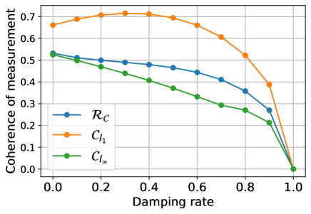
Figure 1: $\mathcal{R}_{\mathcal{C}}$, $\mathcal{C}_{l_{1}}$ and $\mathcal{C}_{l_{\infty}}$ for a dichotomic POVM $\mathbf{G}$ in a 3-dimensional system $\mathbf{G}\in\mathcal{M}(3,2)$ to which the amplitude damping channel is applied. Detailed POVM components are given in F.

4 Experimental scheme to assess coherence of measurement

General procedures for detector tomography consist of two steps: (i) data collection as preparing a set of probe states and measuring each of them by an unknown measurement and (ii) data analysis, the so-called global reconstruction as finding the optimal physical POVM consistent with the data [50]. However, the global reconstruction can be challenging for high dimensional systems. We instead employ a procedure introduced in [39] for quantum process tomography. For an unknown measurement $\mathbf{A}=\{A_{a}\}_{a=0}^{n-1}$ on $\mathcal{H}_{d}$, a set of $d^{2}$ linearly independent probe states $\{\rho_{k}\}_{k=1}^{d^{2}}$ is required to explicitly obtain $\mathbf{A}$. We denote by $p(a|k)$ the probability of obtaining outcome $a$ associated with the POVM $\mathbf{A}$ for a probe state $\rho_{k}$. Without loss of generality, we write them in an incoherent basis as $A_{a}=\sum_{i,j=0}^{d-1}\alpha_{ij|a}|i\rangle\langle j|$ and $\rho_{k}=\sum_{i,j=0}^{d-1}\beta_{ij|k}|i\rangle\langle j|$, where $\alpha_{ij|a}=\langle i|A_{a}|j\rangle$ and $\beta_{ij|k}=\langle i|\rho_{k}|j\rangle$, respectively. Each probability is written in terms of $\alpha_{ij|a}$ and $\beta_{ij|k}$ as $p(a|k)=\Tr[\rho_{k}A_{a}]=\sum_{i,j=0}^{d-1}\beta_{ij|k}\alpha_{ji|a}$ for all $a$ and $k$.

We introduce $d^{2}$-dimensional real column vectors $\bm{\gamma}_{k}$ and $\bm{\chi}_{a}$ that contain information on $\rho_{k}$ and $A_{a}$, respectively. That is, we can rewrite $p(a|k)$ as

$$p(a|k)={\bm{\gamma}}_{k}^{T}\bm{\chi}_{a},$$ (13)

where $\bm{\chi}_{a}$ and $\bm{\gamma}_{k}$ are defined as

$$(\bm{\chi}_{a})_{x}=\begin{cases}\alpha_{qq|a}&\text{for }q=r\\ \sqrt{2}\text{Re}[\alpha_{qr|a}]&\text{for }q<r\\ \sqrt{2}\text{Im}[\alpha_{rq|a}]&\text{for }q>r\end{cases},$$

$$(\bm{\gamma}_{k})_{x}=\begin{cases}\beta_{qq|k}&\text{for }q=r\\ \sqrt{2}\text{Re}[\beta_{qr|k}]&\text{for }q<r\\ \sqrt{2}\text{Im}[\beta_{rq|k}]&\text{for }q>r\end{cases}$$

with integers $0\leq x\leq d^{2}-1$ and $0\leq q,r\leq d-1$ holding $x=qd+r$. For instance, we have $\bm{\gamma}_{k}=(\beta_{00|k},\sqrt{2}\text{Re}[\beta_{01|k}],\sqrt{2}\text{Im}[\beta_{01|k}],\beta_{11|k})^{T}$ for $d=2$. Then, as we define $d^{2}\times d^{2}$ square matrix as $\bm{\Gamma}=(\bm{\gamma}_{1},\bm{\gamma}_{2},...,\bm{\gamma}_{d^{2}})$ and a probability vector for $a$ as $\bm{\mu}_{a}=(p(a|1),...,p(a|d^{2}))^{T}$, all measured statistics related to an outcome $a$ is written in terms of these vectors as

$$\bm{\Gamma}^{T}\bm{\chi}_{a}=\bm{\mu}_{a}.$$ (14)

Linear independence of $\rho_{k}$ implies that the inverse of $\bm{\Gamma}$ exists. Therefore, by applying its inverse $(\bm{\Gamma}^{T})^{-1}$ on both sides, one can obtain the unknown vector $\bm{\chi}_{a}$ that explicitly determines the POVM component $A_{a}$.

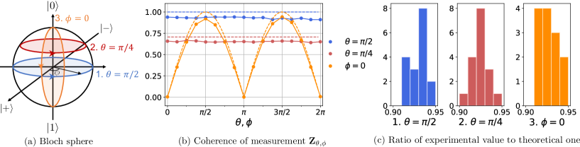
Figure 2: Demonstration for single qubit measurements on IBM Quantum systems. (a) Each point in the Bloch sphere represents the direction of measurement $\mathbf{Z}_{\theta,\phi}$ varying along the different paths. (b) Coherence of measurements $\mathbf{Z}_{\theta,\phi}$ along paths 1 (blue), 2 (red) and 3 (orange). Dashed curves show theoretical expectation values. (c) Histograms of the ratio of an experimental value to the theoretical one.

For our goal to experimentally assess the coherence of measurements, we consider the following family of linearly independent states,

$$|\psi_{kl}\rangle=\begin{cases}|k\rangle&\text{for }k=l\\ ({|k\rangle+|l\rangle})/{\sqrt{2}}&\text{for }k>l\\ ({|k\rangle+i|l\rangle})/{\sqrt{2}}&\text{for }k<l\end{cases},$$ (15)

with $k,l=0,\cdots,d-1$. Preparing this family of states and measuring them by an unknown POVM $\mathbf{A}$, one can directly construct the components of a POVM from the relations

$$p(a|kl)-\frac{p(a|kk)+p(a|ll)}{2}=\begin{cases}\text{Re}[\langle k|A_{a}|l\rangle]&\text{ for }k>l\\ \text{Im}[\langle l|A_{a}|k\rangle]&\text{ for }k<l\end{cases},$$

where we denote a probability to obtain an outcome $a$ for a prepared state $|\psi_{kl}\rangle$ by $p(a|kl)=\langle\psi_{kl}|A_{a}|\psi_{kl}\rangle$. The benefit of this method is that one can avoid the reconstruction of whole POVM components that may be challenging for high dimensional systems. In addition, it is possible to obtain its off-diagonal elements, $\langle k|A_{a}|l\rangle$ straightforwardly, and also to measure it selectively by preparing $|\psi_{kl}\rangle$ for specific values of $k,l$. Here, the quantum superposition of $|k\rangle$ and $|l\rangle$ serves as a resource to assess the amount of coherence in that basis.

We demonstrate our proposed scheme in a single qubit experiment on the 20 qubit IBM Quantum system “Singapore”. In the IBM Q processor, qubit states are measured in computational basis, i.e., $\mathbf{Z}=\{|0\rangle,|1\rangle\}$. We manipulate measurement basis by applying the following single-qubit gate before measuring in $\mathbf{Z},$

$$V_{\theta,\phi}=\begin{pmatrix}\cos(\theta/2)&&e^{-i\phi}\sin(\theta/2)\\ -\sin(\theta/2)&&e^{-i\phi}\cos(\theta/2)\end{pmatrix},$$

with the polar angle $\theta\in[0,\pi]$ and the azimuthal angle $\phi\in[0,2\pi]$. As a result, it is equivalent to execute the measurement $\mathbf{Z}_{\theta,\phi}=\{V_{\theta,\phi}^{\dagger}|0\rangle,V_{\theta,\phi}^{\dagger}|1\rangle\}$. To assess its coherence of measurement, we prepare the family of states $\{|\psi_{kl}\rangle\}_{k,l=0,1}$ as specified in (15). In the IBM Q processor, they are prepared by applying appropriate single-qubit gates to the initial state $|0\rangle$ (see G for more details).

We consider three cases $(i)\;\theta=\pi/2$, $(ii)\;\theta=\pi/4$ and $(iii)\;\phi=0$ as illustrated in figure 2-(a). For the cases $(i)\;\theta=\pi/2$ and $(ii)\;\theta=\pi/4$, we vary $\phi\in[0,2\pi]$ with an interval of $\pi/8$. Similarly, for the case $(iii)\;\phi=0$, we vary $\theta\in[0,2\pi]$ with an interval of $\pi/8$ . For the single qubit measurement $\mathbf{Z}_{\theta,\phi}$, its coherence of measurement is given by $\mathcal{R}(\mathbf{Z}_{\theta,\phi})=\mathcal{C}_{l_{\infty}}(\mathbf{Z}_{\theta,\phi})=\mathcal{C}_{l_{1}}(\mathbf{Z}_{\theta,\phi})/2=|\sin\theta|$ according to (12). We plot its theoretical and experimental values in figure 2-(b). Here, each point denotes the average value of 10 runs with the setting of 8192 shots for each run on the IBM Q processor. For each point, the order of its standard deviation is less than $10^{-3}$, so that its error bar is smaller than the size of a point.

In figure 2-(b), the gap between experimental and theoretical values seems to be bigger with a larger coherence of measurement. In order to see this trend more clearly, we draw histograms for the ratio of each experimental value to its theoretical one except for singular points where theoretical values become zero, i.e., $\theta=0,\pi,2\pi$ for $\phi=0$. The corresponding histograms in figure 2-(c) show that the ratios are rather uniform in the range of 0.9 $\sim$ 0.95 insensitive to the degree of coherence.

In practice, our experimental results were obtained by executing designed circuits in IBM Q processor and the prepared states would not be pure. However, we may assign the error or noise occurring to these probe states to the POVM under test. That is, we assume a pure probe state for analysis in Eq. (17) (Eq. (14) in the revised version), and importantly, this procedure will only underestimate the coherence of measurement, thereby providing a reliable lower bound for robustness, if the noise occurring is SIO (strictly incoherent operation): When we introduced the properties of our monotone of coherence, we proved that the SIO does not increase the coherence measure. Therefore, it becomes important to understand what kinds of errors actually occur in IBM Q processor.

As addressed in [51], the IBM Q processor has two different types of errors, (i) classical errors from the dcoherence represented by the shrinkage of arrow in the Bloch-vector representation in figure 2-(a), and (ii) nonclassical errors represented by the tilt of measurement directions. In the context of coherence, both errors are critical because coherence is not only sensitive to the decoherence but also basis-dependent. However, two types of errors could cause different effects on measurement coherence. For instance, the classical errors lead to uniform decrease of coherence regardless of measurement directions, while the nonclassical ones lead to different behaviors of coherence depending on measurement directions. Therefore, classical errors seem to be dominant in our experimental data, because the ratios of experimental values to theoretical ones are rather uniform in the range from 0.9 to 0.95 regardless of measurement directions. We thus attribute this trend to classical errors occurring in the machine, which could be further confirmed through other related experiments [51].

5 Conclusion

In summary, we have explored how to quantify coherence of measurement in a resource theoretical framework. A resource theory generally consists of two ingredients, free resources and free operations. In this work, we defined a free resource as an incoherent measurement (4) by which one cannot give access to coherence of states experimentally. We also defined a free operation as a strictly incoherent operation (SIO) that cannot create a coherent measurement from an incoherent one. We remark that the SIOs are known as a physically well-motivated set of free operations for coherence, as one can neither create nor use coherence via a SIO [41, 21]. In this framework, we showed that a statistical distance can be used to define a coherence monotone of measurements (6). In particular, the relative entropy gives us a monotone that fulfills all postulates ($\mathcal{C}$1)-($\mathcal{C}$4). On the other hand, we introduced the $l_{\infty}$ norm-based coherence monotone $\mathcal{C}_{l_{\infty}}$ that is determined by off-diagonal elements of each POVM component. It can therefore be readily calculated without the convex optimization. Furthermore, we showed that $\mathcal{C}_{l_{\infty}}$ gives a lower bound on the robustness measure $\mathcal{R}_{C}$ in (12) and they become identical for two-outcome POVMs on $\mathcal{H}_{2}$.

To address the coherence of measurement experimentally, we need to have a full description of a given POVM. To this end, we introduced a procedure for the detector tomography by adopting the quantum process tomography [39]. In this procedure, $d^{2}$ linearly independent probe states are prepared and each probe state is measured by an unknown measurement. Then one can obtain its full description from the relation (14). One of advantages from this procedure is that it can be implemented without the global reconstruction that may require a demanding numerical computation. Furthermore, as we prepare a particular set of probe states (15), we obtain the off-diagonal elements of each POVM component straightforwardly and selectively. Finally, we illustrated the feasibility of our approach by performing the single qubit experiment on the 20 qubit IBM Quantum system ”Singapore” as shown in figure 2.

We hope that our work could lead to further researches on quantitatively characterizing the role of coherence of measurements in operational tasks such as quantum measurement engine and measurement-based quantum computation. From the fundamental perspective, our approach may provide some insights to exploring other characteristics of quantum measurements such as incompatibility and separable measurements, which will be all subject to future studies.

Appendix A Strictly incoherent operation [41, 21]

An incoherent Kraus operator is generally written as [42]

$$K_{\mu}=\sum_{i=0}^{d-1}c_{\mu,i}|f_{\mu}(i)\rangle\langle i|$$

with coefficients satisfying the completeness relation

$$\sum_{\mu:f_{\mu}(i)=f_{\mu}(j)}c_{\mu,j}^{*}c_{\mu,i}=\delta_{ij},$$

where $f_{\mu}$ is a function from $\{0,...,d-1\}$ to $\{0,...,d-1\}$. The conjugate of $K_{\mu}$ must also be written in this form to be a strictly incoherent operation. It implies $f_{\mu}$ should be an invertible function, i.e., permutation $\pi_{\mu}$ depending on $\mu$ [42]. In this case, the Kraus operator can be decomposed as

$$K_{\mu}=\sum_{i=0}^{d-1}c_{\mu,i}|\pi_{\mu}(i)\rangle\langle i|=\sum_{i=0}^{d-1}c_{\mu,i}{V}_{\mu}|i\rangle\langle i|={V}_{\mu}\tilde{K}_{\mu},$$

where $V_{\mu}$ is an unitary operation corresponding to the permutation $\pi_{\mu}$ and $\tilde{K}_{\mu}=\sum_{i=0}^{d-1}c_{\mu,i}|i\rangle\langle i|$ is a genuinely incoherent Kraus operator [21]. Here, the coefficients satisfy $\sum_{\mu}|c_{\mu,i}|^{2}=1$ for the completeness relation.

A.1 Dual of a selective operation

In the condition ($\mathcal{C}$3), we have the measurement $\mathbf{A}^{\prime}=\{K_{\mu}^{\dagger}A_{a}K_{\mu}\}$, which is given after applying the dual operation of a selective SIO to $\mathbf{A}$. To explain it more specifically, let us introduce an ancilla storing classical information about the selection $\mu$. We assume an operation $\mathcal{E}$ given by $\{K_{\mu}\otimes U_{\mu}^{cl}\}_{\mu=0}^{n_{\mathcal{E}}-1}$ acts on a quantum state $\rho\otimes|0\rangle\langle 0|^{cl}$, where $K_{\mu}$ is a Kraus operator and $U_{\mu}^{cl}$ is an unitary operator shifting the basis $\{|i\rangle^{cl}\}_{i=0}^{n_{\mathcal{E}}-1}$ by $\mu$, i.e., $U_{\mu}^{cl}|i\rangle^{cl}=|i+\mu\text{ mod }n_{\mathcal{E}}\rangle^{cl}$ in $n_{\mathcal{E}}$-dimensional Hilbert space. By applying $\mathcal{E}$ to the state, we have

$$\mathcal{E}(\rho\otimes|0\rangle\langle 0|^{cl})=\sum_{\mu=0}^{n_{\mathcal{E}}-1}K_{\mu}\rho K_{\mu}^{\dagger}\otimes|\mu\rangle\langle\mu|^{cl}.$$

Then, we can make a selective operation on the initial measurement by performing a measurement given by $\{A_{a}\otimes|i\rangle\langle i|^{cl}\}_{a\in\mathcal{Z}_{n},i\in\mathcal{Z}_{n_{\mathcal{E}}}}$, where $\mathcal{Z}_{n}=\{0,1,...,n-1\}$. As a result, this measurement gives a distribution $p(m,\mu)=\Tr[K_{\mu}\rho K_{\mu}^{\dagger}A_{a}]$. This result is equivalent to what we would obtain by measuring $\rho$ via $\{K_{\mu}^{\dagger}A_{a}K_{\mu}\}_{a\in\mathcal{Z}_{n},\mu\in\mathcal{Z}_{n_{\mathcal{E}}}}$. Therefore, we can consider $\mathbf{A}^{\prime}$ as a measurement given after applying the dual operation of a selective SIO.

Appendix B Proofs of conditions for $\mathcal{C}_{D}(A)$ and $\mathcal{C}_{S}(A)$

We first prove that $\mathcal{C}_{D}(\mathbf{A})$ satisfies ($\mathcal{C}$1) and ($\mathcal{C}$2) as follows.

Proof of ($\mathcal{C}$1) for $\mathcal{C}_{D}(\mathbf{A})$. Any statistical distance is supposed to give $D(\mathbf{A},\mathbf{M})=0$ if and only if two probability distributions associated with POVMs $\mathbf{A}$ and $\mathbf{M}$ are identical. Otherwise it should be strictly positive. Thus, in the definition of $\mathcal{C}_{D}(\mathbf{A})$, $\sup_{\rho}D(\mathbf{A},\mathbf{M})=0$ implies that two probability distributions are identical for all states, i.e., $\Tr[\rho A_{a}]=\Tr[\rho M_{a}]$ for arbitrary $a$ and $\rho$. Equivalently, it can be said that $\mathbf{A}$ and $\mathbf{M}$ are identical. Thus, if $\mathbf{A}$ is an incoherent measurement, $\mathcal{C}_{D}(\mathbf{A})$ vanishes during the minimization over all incoherent measurements. Otherwise, it gives a strict positive value. ∎

Proof of ($\mathcal{C}$2) for $\mathcal{C}_{D}(\mathbf{A})$. If $\mathcal{E}$ is a SIO, then we have

$$\mathcal{C}_{D}(\mathbf{A}) =\min_{\mathbf{M}\in\mathcal{I}(d,n)}\sup_{\rho}D_{\rho}(\mathbf{A},\mathbf{M})$$

$$\geq\min_{\mathbf{M}\in\mathcal{I}(d,n)}\sup_{\mathcal{E}(\rho)}D_{\mathcal{E}(\rho)}(\mathbf{A},\mathbf{M})$$

$$=\min_{\mathbf{M}\in\mathcal{I}(d,n)}\sup_{\rho}D_{\rho}(\mathcal{E}^{*}(\mathbf{A}),\mathcal{E}^{*}(\mathbf{M}))$$

$$\geq\min_{\mathbf{M}\in\mathcal{I}(d,n)}\sup_{\rho}D_{\rho}(\mathcal{E}^{*}(\mathbf{A}),\mathbf{M})=\mathcal{C}_{D}(\mathcal{E}^{*}(\mathbf{A})).$$

Here, the first inequality comes from the fact that $\{\mathcal{E}(\rho)|\text{ for all }\rho\}$ is a subset of $\{\rho\}$. Similarly, we have the second inequality due to $\{\mathcal{E}^{*}(\mathbf{M})|\mathbf{M}\in\mathcal{I}(d,n)\}\subset\mathcal{I}(d,n)$. ∎

Furthermore, the convexity of a statistical distance $D$ implies the convexity of $\mathcal{C}_{D}$, which is proved as follows.

Proof of ($\mathcal{C}$4) for $\mathcal{C}_{D}(\mathbf{A})$ with the convexity of $D$. Let us assume the convexity of $D$. That is, for pairs of probability distributions $(p_{\mathbf{A}_{k}},p_{\mathbf{M}_{k}})$ associated with measurements $\mathbf{A}_{k}$ and $\mathbf{M}_{k}$, respectively, we have $D(\sum_{k}q_{k}\mathbf{A}_{k},\sum_{k}q_{k}\mathbf{M}_{k})\leq\sum_{k}q_{k}D(\mathbf{A}_{k},\mathbf{M}_{k})$ with the probability $q_{k}$. By using this property, we have

$$\mathcal{C}_{D}(\sum_{k}q_{k}\mathbf{A}_{k}) =\min_{\mathbf{M}_{k}\in\mathcal{I}(d,n)}\sup_{\rho}D_{\rho}(\sum_{k}q_{k}\mathbf{A}_{k},\sum_{k}q_{k}\mathbf{M}_{k})$$

$$\leq\min_{\mathbf{M}_{k}\in\mathcal{I}(d,n)}\sup_{\rho}\sum_{k}q_{k}D_{\rho}(\mathbf{A}_{k},\mathbf{M}_{k})$$

$$\leq\sum_{k}q_{k}\min_{\mathbf{M}_{k}\in\mathcal{I}(d,n)}\sup_{\rho}D_{\rho}(\mathbf{A}_{k},\mathbf{M}_{k})$$

$$=\sum_{k}q_{k}\mathcal{C}_{D}(\mathbf{A}_{k}).$$

In the first line, one can write the minimization over $\sum_{k}q_{k}\mathbf{M}_{k}$ without loss of generality. Then, the first inequality comes from the convexity of $D$ and the second one is given by taking supremum for each distance. ∎

According to the above proofs, $\mathcal{C}_{S}$ holds the conditions ($\mathcal{C}$1-2) and ($\mathcal{C}$4) due to its positive definiteness and convexity. Let us prove the satisfaction of ($\mathcal{C}$3) for $\mathcal{C}_{S}$ in the following.

Proof of ($\mathcal{C}$3) for $\mathcal{C}_{S}(\mathbf{A})$. Let a selective SIO $\mathcal{E}$ be described by a set of Kraus operators $\{K_{\mu}\}_{\mu=0}^{n_{\mathcal{E}}-1}$. Then, we have the following relations for $\mathbf{A}\in\mathcal{M}(d,n)$.

$$\min_{\mathbf{M}\in\mathcal{I}(d,n)}\sup_{\rho}S_{\rho}(\mathbf{A}\|\mathbf{M})$$

$$\geq\min_{\mathbf{M}\in\mathcal{I}(d,n)}\sup_{\rho}\left(\sum_{\mu=0}^{n_{\mathcal{E}}-1}p_{\mu}S_{\rho_{\mu}}(\mathbf{A}\|\mathbf{M})\right)$$

$$=\min_{\mathbf{M}\in\mathcal{I}(d,n)}\sup_{\rho}\left(\sum_{\mu=0}^{n_{\mathcal{E}}-1}p_{\mu}\sum_{a=0}^{n-1}p_{\mathbf{A}}(a|\mu)\log\frac{p_{\mathbf{A}}(a|\mu)}{p_{\mathbf{M}}(a|\mu)}\right)$$

$$=\min_{\mathbf{M}\in\mathcal{I}(d,n)}\sup_{\rho}\left(\sum_{\mu=0}^{n_{\mathcal{E}}-1}\sum_{a=0}^{n-1}p_{\mu}p_{\mathbf{A}}(a|\mu)\log\frac{p_{\mu}p_{\mathbf{A}}(a|\mu)}{p_{\mu}p_{\mathbf{M}}(a|\mu)}\right)$$

$$=\min_{\mathbf{M}\in\mathcal{I}(d,n)}\sup_{\rho}\left(\sum_{\mu=0}^{n_{\mathcal{E}}-1}\sum_{a=0}^{n-1}\Tr[K_{\mu}\rho K_{\mu}^{\dagger}A_{a}]\log\frac{\Tr[K_{\mu}\rho K_{\mu}^{\dagger}A_{a}]}{\Tr[K_{\mu}\rho K_{\mu}^{\dagger}M_{a}]}\right)$$

$$=\min_{\mathbf{M}\in\mathcal{I}(d,n)}\sup_{\rho}\left(\sum_{\mu=0}^{n_{\mathcal{E}}-1}\sum_{a=0}^{n-1}\Tr[\rho K_{\mu}^{\dagger}A_{a}K_{\mu}]\log\frac{\Tr[\rho K_{\mu}^{\dagger}A_{a}K_{\mu}]}{\Tr[\rho K_{\mu}^{\dagger}M_{a}K_{\mu}]}\right)$$

$$=\min_{\mathbf{M}\in\mathcal{I}(d,n)}\sup_{\rho}S(\mathbf{A}^{\prime}\|\mathbf{M}^{\prime})$$

$$\geq\min_{\mathbf{M}\in\mathcal{I}(d,n\cdot n_{\mathcal{E}})}\sup_{\rho}S(\mathbf{A}^{\prime}\|\mathbf{M})$$

where a conditional state $\rho_{\mu}=K_{\mu}\rho K_{\mu}^{\dagger}/p_{\mu}$ is obtained with the probability $p_{\mu}=\Tr[K_{\mu}\rho K_{\mu}^{\dagger}]$ after applying $\mathcal{E}$ to $\rho$. Here, the first inequality comes from $\sup_{\rho}S_{\rho}(\mathbf{A}\|\mathbf{M})\geq\sup_{\rho}S_{\rho_{\mu}}(\mathbf{A}\|\mathbf{M})$ because $\{\rho_{\mu}|\forall\rho\}$ is a subset of density operators on $\mathcal{H}_{d}$. Before the second inequality, we denote the POVMs emerging after applying the dual of the seletive SIO $\mathcal{E}$ to $\mathbf{M}\in\mathcal{I}({d,n})$ by $\mathbf{M}^{\prime}=\{K_{\mu}^{\dagger}M_{a}K_{\mu}\}_{a,\mu}\in\mathcal{I}({d,n\cdot n_{\mathcal{E}}})$. Because $\mathbf{M}^{\prime}$ defines a subset of incoherent measurements in $\mathcal{I}({d,n\cdot n_{\mathcal{E}}})$, the minimization over all incoherent measurement on $\mathcal{I}(d,n\cdot n_{\mathcal{E}})$ gives a smaller value. Note that this proof is applicable to other statistical distances if they satisfy $\sum_{\mu=0}^{n_{\mathcal{E}}-1}p_{\mu}D_{\rho_{\mu}}(\mathbf{A}\|\mathbf{M})=D_{\rho}(\mathbf{A}^{\prime}\|\mathbf{M}^{\prime})$. ∎

Appendix C Proofs of conditions for $\mathcal{C}(\mathbf{A})$

We prove that $\mathcal{C}_{l_{\infty}}(\mathbf{A})$ satisfies requirements ($\mathcal{C}$1-4) as follows.

Proof of ($\mathcal{C}$1) for $\mathcal{C}_{l_{\infty}}(\mathbf{A})$. If a POVM $\mathbf{A}\in\mathcal{M}(d,n)$ is incoherent, then $|\langle i|A_{a}|j\rangle|=0$ for all $i,j$ and $a$, and vice versa. ∎

Proof of ($\mathcal{C}$2) for $\mathcal{C}_{l_{\infty}}(\mathbf{A})$. $\mathcal{C}_{l_{\infty}}(\mathbf{A})$ is independent of phase factors. Thus, without loss of generality, we assume that Kraus operators of a SIO $\mathcal{E}$ are given as

$$K_{\mu}=\sum_{i=0}^{d-1}\sqrt{p_{\mu|i}}|\pi_{\mu}(i)\rangle\langle i|.$$ (16)

Then, applying the dual of $\mathcal{E}$ gives rise to

$$\mathcal{E}^{*}(\mathbf{A})=\left\{\sum_{\mu=0}^{n_{\mathcal{E}}-1}\sum_{i,j=0}^{d-1}\sqrt{p_{\mu|i}p_{\mu|j}}\langle\pi_{\mu}(i)|A_{a}|\pi_{\mu}(j)\rangle|i\rangle\langle j|\right\}_{a=0}^{n-1}.$$

Its coherence monotone $\mathcal{C}$ becomes smaller as follows:

$$\mathcal{C}_{l_{\infty}}(\mathcal{E}^{*}(\mathbf{A})) =\max_{i<j}\sum_{a=0}^{n-1}\left|\sum_{\mu=0}^{n_{\mathcal{E}}-1}\sqrt{p_{\mu|i}p_{\mu|j}}\langle\pi_{\mu}(i)|A_{a}|\pi_{\mu}(j)\rangle\right|$$

$$\leq\max_{i<j}\sum_{\mu=0}^{n_{\mathcal{E}}-1}\sqrt{p_{\mu|i}p_{\mu|j}}\sum_{a=0}^{n-1}\left|\langle\pi_{\mu}(i)|A_{a}|\pi_{\mu}(j)\rangle\right|$$

$$\leq\mathcal{C}_{l_{\infty}}(\mathbf{A})\max_{i<j}\sum_{\mu=0}^{n_{\mathcal{E}}-1}\sqrt{p_{\mu|i}p_{\mu|j}}$$

$$\leq\mathcal{C}_{l_{\infty}}(\mathbf{A}).$$

The first inequality is due to the subadditivity of the absolute value. We have the second inequality by the definition of $\mathcal{C}_{l_{\infty}}$. The third inequality comes out of the Cauchy–Schwarz inequality. ∎

Proof of ($\mathcal{C}$3) for $\mathcal{C}_{l_{\infty}}(\mathbf{A})$. For the same reason as above, we again restrict ourselves without loss of generality to a selective SIO $\mathcal{E}$ described by Kraus operators in (16). Then applying it to $\mathbf{A}\in\mathcal{M}(d,n)$, we have the POVM $\mathbf{A}^{\prime}=\{K_{\mu}^{\dagger}A_{a}K_{\mu}\}\in\mathcal{M}(d,n\cdot n_{\mathcal{E}})$, where each POVM component is expanded as

$$K_{\mu}^{\dagger}A_{a}K_{\mu}=\sum_{i,j=0}^{d-1}\sqrt{p_{\mu|i}p_{\mu|j}}\langle\pi_{\mu}(i)|A_{a}|\pi_{\mu}(j)\rangle|i\rangle\langle j|.$$

Its coherence monotone $\mathcal{C}_{l_{\infty}}$ is given as

$$\mathcal{C}_{l_{\infty}}(\mathbf{A}^{\prime}) =\max_{i<j}\sum_{\mu=0}^{n_{\mathcal{E}}-1}\sum_{a=0}^{n-1}\left|\sqrt{p_{\mu|i}p_{\mu|j}}\langle\pi_{\mu}(i)|A_{a}|\pi_{\mu}(j)\rangle\right|.$$

In the same way that we prove ($\mathcal{C}$2) for $\mathcal{C}_{l_{\infty}}$, the Cauchy-Schwarz inequality implies the monotonicity $\mathcal{C}_{l_{\infty}}(\mathbf{A}^{\prime})\leq\mathcal{C}_{l_{\infty}}(\mathbf{A}).$ ∎

Proof of ($\mathcal{C}$4) for $\mathcal{C}_{l_{\infty}}(\mathbf{A})$. We consider the convex combination of $\mathbf{A},\mathbf{B}\in\mathcal{M}(d,n)$ that is the POVM $p\mathbf{A}+(1-p)\mathbf{B}=\{pA_{a}+(1-p)B_{a}\}_{a=0}^{n-1}$ with weight $p$. Then its coherence monotone $\mathcal{C}_{l_{\infty}}$ is given as

$$\mathcal{C}_{l_{\infty}}(p\mathbf{A}+(1-p) \mathbf{B})=\max_{i<j}\sum_{a=0}^{n-1}\left|\langle i|pA_{a}+(1-p)B_{a}|j\rangle\right|$$

$$\leq \max_{i<j}\sum_{a=0}^{n-1}\big{(}p\left|\langle i|A_{a}|j\rangle|+(1-p)|\langle i|B_{a}|j\rangle\right|\big{)}$$

$$\leq p\mathcal{C}_{l_{\infty}}(\mathbf{A})+(1-p)\mathcal{C}_{l_{\infty}}(\mathbf{B}).$$

Here, the first inequality comes from the subadditivity of the absolute value, and the second one by separately applying the maximization. ∎

Appendix D A counter example of the monotonicity for $\mathcal{C}_{l_{1}}$

We show that $\mathcal{C}_{l_{1}}$ does not fulfill the monotonicity ($\mathcal{C}$2) by a counter example. Let us consider a POVM $\mathbf{A}=\{A_{\pm}\}\in\mathcal{M}(4,2)$, where POVM components are given by

$$A_{\pm}=\begin{pmatrix}1/2&\pm 1/2&0&0\\ \pm 1/2&1/2&0&0\\ 0&0&1/2&0\\ 0&0&0&1/2\end{pmatrix}.$$

Then, as we apply the dual of a SIO $\mathcal{E}$ described by the Kraus operators

$$K_{0}=\begin{pmatrix}1&0&0&0\\ 0&1&0&0\\ 0&0&0&0\\ 0&0&0&0\end{pmatrix},K_{1}=\begin{pmatrix}0&0&1&0\\ 0&0&0&1\\ 0&0&0&0\\ 0&0&0&0\end{pmatrix},$$

the POVM components become

$$\mathcal{E}^{*}(A_{\pm})=\begin{pmatrix}1/2&\pm 1/2&0&0\\ \pm 1/2&1/2&0&0\\ 0&0&1/2&\pm 1/2\\ 0&0&\pm 1/2&1/2\end{pmatrix},$$

respectively. Consequently, one can easily identify that $\mathcal{C}_{l_{1}}(\mathbf{A})=2\leq\mathcal{C}_{l_{1}}(\mathcal{E}^{*}(\mathbf{A}))=4$.

Appendix E Proof of Theorem 1

To prove Theorem 1, we need the following lemma.

Lemma 1.

For any state $\rho$ on $\mathcal{H}_{d}$, its off-diagonal elements satisfy

$$|\langle i|\rho|j\rangle|\leq\frac{1}{2}\text{ for }i\neq j.$$ (17)

Proof.

A state $\rho$ is positive semidefinite if and only if the determinant of every submatrix indexed by the same rows and columns of $\rho$, i.e., every principal submatrix of $\rho$, is nonnegative [52]. Thus, the determinant of any $2\times 2$ submatrix $\rho(i,j)$ of $\rho$ given by

$$\rho(i,j)=\begin{pmatrix}\rho_{ii}&\rho_{ij}\\ \rho_{ji}&\rho_{jj}\end{pmatrix},$$

must be non-negative, namely $\sqrt{\rho_{ii}\rho_{jj}}\geq|\rho_{ji}|$, where $\rho_{ij}\equiv\langle i|\rho|j\rangle$. The Cauchy-Schwarz inequality with $\rho_{ii}+\rho_{jj}\leq 1$ and $\rho_{ii}\geq 0$ for any $i,j$ then implies $|\rho_{ji}|\leq 1/2$. ∎

Proof of Theorem 1.

The robustness is efficiently cast by using semidefinite programming(SDP), and particularly in our case its dual problem is written as the following SDP [35].

$$maximize \;\;\;\;\;\sum_{a=0}^{n-1}\Tr[Z_{a}A_{a}]-1$$ (18)

$$subject\;to \;\;\;\;\;\forall i,a\;\;\;Z_{a}\geq 0,\;\;\langle i|Z_{a}|i\rangle=\langle i|Z_{n}|i\rangle$$ (19)

$$\;\;\;\;\;\Tr[Z_{n}]=1.$$ (20)

To prove the lower bound, let us rewrite the maximized function (18) as

$$\sum_{a=0}^{n-1}\Tr[Z_{a}A_{a}]-1=\sum_{a=0}^{n-1}\sum_{i,j=0}^{d-1}\langle i|Z_{a}|j\rangle\langle j|A_{a}|i\rangle-1$$

$$=\sum_{i=0}^{d-1}\sum_{a=0}^{n-1}\langle i|Z_{a}|i\rangle\langle i|A_{a}|i\rangle+\sum_{i\neq j}^{d-1}\sum_{a=0}^{n-1}\langle i|Z_{a}|j\rangle\langle j|A_{a}|i\rangle-1$$

$$=\sum_{i\neq j}^{d-1}\sum_{a=0}^{n-1}\langle i|Z_{a}|j\rangle\langle j|A_{a}|i\rangle.$$ (21)

Here, we have the third equality by using the completeness of $\mathbf{A}$ with the fact that $\langle i|Z_{a}|i\rangle$ is independent of $a$ as specified in Eq. (19).

Now, consider a set of states $\{|k,l,\theta_{a}\rangle\}_{a=0}^{n-1}$ given by

$$|k,l,\theta_{a}\rangle=\frac{1}{\sqrt{2}}(|k\rangle+e^{i\theta_{a}}|l\rangle),$$ (22)

which defines $Z_{a}\equiv|k,l,\theta_{a}\rangle\langle k,l,\theta_{a}|$ to be used in Eq. (E). The last term in Eq. (E) is then given by

$$\sum_{i\neq j}^{d-1}\sum_{a=0}^{n-1}\langle i|Z_{a}|j\rangle\langle j|A_{a}|i\rangle=\sum_{a=0}^{n-1}{Re}\left[e^{i\theta_{a}}\langle l|A_{a}|k\rangle\right].$$ (23)

Let $\mathcal{C}_{l_{\infty}}(\mathbf{A})=\max_{i,j}\sum_{a=0}^{n-1}|\langle i|A_{a}|j\rangle|$ be achieved by $\{i,j\}=\{k,l\}$. Setting $\theta_{a}\equiv-\arg[\langle l|A_{a}|k\rangle]$, we see that (23) becomes $\mathcal{C}_{l_{\infty}}(\mathbf{A})$. This proves $\mathcal{C}_{l_{\infty}}(\mathbf{A})\leq\mathcal{R}_{C}(\mathbf{A})$, as $\mathcal{C}_{l_{\infty}}(\mathbf{A})$ can always be achieved by choosing a certain set of states $Z_{a}$ in (22).

It is straightforward to prove the upper bound, as we apply the result of lemma 1 to (E) as

$$\sum_{i\neq j}^{d-1}\sum_{a=0}^{n-1}\langle i|Z_{a}|j\rangle\langle j|A_{a}|i\rangle$$

$$\leq\sum_{i\neq j}^{d-1}\sum_{a=0}^{n-1}|\langle i|Z_{a}|j\rangle||\langle j|A_{a}|i\rangle|$$

$$\leq\frac{1}{2}\sum_{i\neq j}^{d-1}\sum_{a=0}^{n-1}|\langle j|A_{a}|i\rangle|=\frac{1}{2}\mathcal{C}_{l_{1}}(\mathbf{A}).$$

This completes the proof. ∎

Appendix F A POVM $\mathbf{M}\in\mathcal{M}(3,2)$ and amplitude damping channel

To see relationships among $\mathcal{R}_{\mathcal{C}}$, $\mathcal{C}_{l_{\infty}}$ and $\mathcal{C}_{l_{1}}$ for higher dimensions, we consider a dichotomic POVM $\mathbf{G}=\{G_{0},G_{1}=I_{3}-G_{0}\}$ as an example in a 3-dimensional system, where the POVM component is defined as

$$G_{0}=\begin{pmatrix}0.528&0.263&0.042\\ 0.263&0.137&0.026\\ 0.042&0.026&0.008\end{pmatrix}.$$

We assume that the amplitude damping channel is applied to the POVM $\mathbf{M}$, of which Kraus operators are given as

$$K_{\mu}^{AD}=\sum_{i=\mu}^{2}\sqrt{i\choose\mu}\sqrt{(1-\gamma)^{i-\mu}\gamma^{\mu}}|i-\mu\rangle\langle i|$$

for $\mu=0,1,2$, where $\gamma$ is the amplitude damping rate. One can identify that the amplitude damping channel is a SIO as the Kraus operators coincide with the form of Kraus operators describing a SIO (5). In figure 1, we plot $\mathcal{R}_{\mathcal{C}}$, $\mathcal{C}_{l_{\infty}}$ and $\mathcal{C}_{l_{1}}$ of $\mathbf{G}^{\prime}=\{\sum_{\mu=0}^{2}K_{\mu}^{AD\dagger}G_{g}K_{\mu}^{AD}\}_{g=0,1}$ versus the damping rate $\gamma$.

Appendix G Experimental data from the IBM Q processor

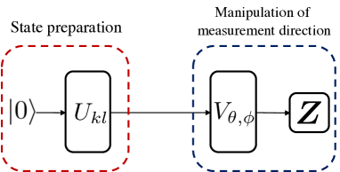
Figure 3: State preparation and manipulation of measurement direction on IBM Q processor.

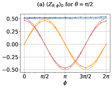
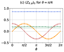
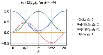
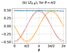
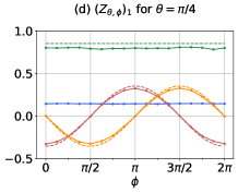
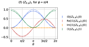
Figure 4: Matrix elements of $(Z_{\theta,\phi})_{i}=V_{\theta,\phi}^{\dagger}|i\rangle\langle i|V_{\theta,\phi}$ for $i=0,1$.

In the IBM Q processor, the initial state is prepared in $|0\rangle$. Applying single-qubit gates $U_{00}=I$, $U_{01}=H$, $U_{10}=PH$ and $U_{11}=X$ to the initial state, we prepare the family of states $\{|\psi_{kl}\rangle=U_{kl}|0\rangle\}_{k,l=0,1}$, where $H=(1/2)(|0\rangle\langle 0|+|0\rangle\langle 1|+|1\rangle\langle 0|-|1\rangle\langle 1|)$, $P=|0\rangle\langle 0|+i|1\rangle\langle 1|$ and $X=|0\rangle\langle 1|+|1\rangle\langle 0|$ are the Hadamard, the phase and the Pauli-$X$ gate, respectively. For each case, we apply the single-qubit gate $V_{\theta,\phi}$ before we execute the measurement $\bm{Z}$, as illustrated in figure 3. Namely, $U_{kl}$ and $V_{\theta,\phi}$ are applied sequentially, with $U_{kl}$ used to prepare $|\psi_{kl}\rangle$ and $V_{\theta,\phi}$ to manipulate the measurement direction.

For a pair of angles $\theta$ and $\phi$, we obtain experimental data for each $k,l$ from the IBM Q processor with the setting of 8192 shots, and calculate the full description of measurement $\bm{Z}_{\theta,\phi}$ from the data. We repeat this procedure 10 times. In figure 4, we plot the average values of matrix elements of POVM components $(Z_{\theta,\phi})_{i}=V_{\theta,\phi}^{\dagger}|i\rangle\langle i|V_{\theta,\phi}$ for $i=0,1$. From these values, we assess coherence of measurements in figure 2 of main text. We also note that the size of standard deviations is less than $10^{-3}$.

References

References

- [1] V. Vedral, M. B. Plenio, M. A. Rippin, and P. L. Knight. Quantifying entanglement. Phys. Rev. Lett., 78:2275–2279, Mar 1997.
- [2] Ryszard Horodecki, Paweł Horodecki, Michał Horodecki, and Karol Horodecki. Quantum entanglement. Rev. Mod. Phys., 81:865–942, Jun 2009.
- [3] A. Grudka, K. Horodecki, M. Horodecki, P. Horodecki, R. Horodecki, P. Joshi, W. Kłobus, and A. Wójcik. Quantifying contextuality. Phys. Rev. Lett., 112:120401, Mar 2014.
- [4] Jiyong Park, Jaehak Lee, Kyunghyun Baek, Se-Wan Ji, and Hyunchul Nha. Faithful measure of quantum non-gaussianity via quantum relative entropy. Phys. Rev. A, 100:012333, Jul 2019.
- [5] Quntao Zhuang, Peter W. Shor, and Jeffrey H. Shapiro. Resource theory of non-gaussian operations. Phys. Rev. A, 97:052317, May 2018.
- [6] Ludovico Lami, Bartosz Regula, Xin Wang, Rosanna Nichols, Andreas Winter, and Gerardo Adesso. Gaussian quantum resource theories. Phys. Rev. A, 98:022335, Aug 2018.
- [7] Francesco Albarelli, Marco G. Genoni, Matteo G. A. Paris, and Alessandro Ferraro. Resource theory of quantum non-gaussianity and wigner negativity. Phys. Rev. A, 98:052350, Nov 2018.
- [8] Ryuji Takagi and Quntao Zhuang. Convex resource theory of non-gaussianity. Phys. Rev. A, 97:062337, Jun 2018.
- [9] Eric Chitambar and Gilad Gour. Quantum resource theories. Rev. Mod. Phys., 91:025001, Apr 2019.
- [10] T. Baumgratz, M. Cramer, and M. B. Plenio. Quantifying coherence. Phys. Rev. Lett., 113:140401, Sep 2014.
- [11] Mark Hillery. Coherence as a resource in decision problems: The deutsch-jozsa algorithm and a variation. Phys. Rev. A, 93:012111, Jan 2016.
- [12] Hai-Long Shi, Si-Yuan Liu, Xiao-Hui Wang, Wen-Li Yang, Zhan-Ying Yang, and Heng Fan. Coherence depletion in the grover quantum search algorithm. Phys. Rev. A, 95:032307, Mar 2017.
- [13] Kamil Korzekwa, Matteo Lostaglio, Jonathan Oppenheim, and David Jennings. The extraction of work from quantum coherence. New Journal of Physics, 18(2):023045, feb 2016.
- [14] Jader P. Santos, Lucas C. Céleri, Gabriel T. Landi, and Mauro Paternostro. The role of quantum coherence in non-equilibrium entropy production. npj Quantum Information, 5(1):23, 2019.
- [15] Iman Marvian and Robert W. Spekkens. How to quantify coherence: Distinguishing speakable and unspeakable notions. Phys. Rev. A, 94:052324, Nov 2016.
- [16] Paolo Giorda and Michele Allegra. Coherence in quantum estimation. Journal of Physics A: Mathematical and Theoretical, 51(2):025302, dec 2017.
- [17] Alexander Streltsov, Uttam Singh, Himadri Shekhar Dhar, Manabendra Nath Bera, and Gerardo Adesso. Measuring quantum coherence with entanglement. Phys. Rev. Lett., 115:020403, Jul 2015.
- [18] Jiajun Ma, Benjamin Yadin, Davide Girolami, Vlatko Vedral, and Mile Gu. Converting coherence to quantum correlations. Phys. Rev. Lett., 116:160407, Apr 2016.
- [19] Kok Chuan Tan, Tyler Volkoff, Hyukjoon Kwon, and Hyunseok Jeong. Quantifying the coherence between coherent states. Phys. Rev. Lett., 119:190405, Nov 2017.
- [20] Alexander Streltsov, Gerardo Adesso, and Martin B. Plenio. Colloquium: Quantum coherence as a resource. Rev. Mod. Phys., 89:041003, Oct 2017.
- [21] Benjamin Yadin, Jiajun Ma, Davide Girolami, Mile Gu, and Vlatko Vedral. Quantum processes which do not use coherence. Phys. Rev. X, 6:041028, Nov 2016.
- [22] Thomas Theurer, Dario Egloff, Lijian Zhang, and Martin B. Plenio. Quantifying operations with an application to coherence. Phys. Rev. Lett., 122:190405, May 2019.
- [23] Adán Cabello. Experimentally testable state-independent quantum contextuality. Phys. Rev. Lett., 101:210401, Nov 2008.
- [24] Piotr Badzia¸g, Ingemar Bengtsson, Adán Cabello, and Itamar Pitowsky. Universality of state-independent violation of correlation inequalities for noncontextual theories. Phys. Rev. Lett., 103:050401, Jul 2009.
- [25] Sixia Yu and C. H. Oh. State-independent proof of kochen-specker theorem with 13 rays. Phys. Rev. Lett., 108:030402, Jan 2012.
- [26] Cyril Elouard, David Herrera-Martí, Benjamin Huard, and Alexia Auffèves. Extracting work from quantum measurement in maxwell’s demon engines. Phys. Rev. Lett., 118:260603, Jun 2017.
- [27] Cyril Elouard, David A. Herrera-Martí, Maxime Clusel, and Alexia Auffèves. The role of quantum measurement in stochastic thermodynamics. npj Quantum Information, 3(1):9, 2017.
- [28] Cyril Elouard and Andrew N. Jordan. Efficient quantum measurement engines. Phys. Rev. Lett., 120:260601, Jun 2018.
- [29] Robert Raussendorf and Hans J. Briegel. A one-way quantum computer. Phys. Rev. Lett., 86:5188–5191, May 2001.
- [30] Robert Raussendorf, Daniel E. Browne, and Hans J. Briegel. Measurement-based quantum computation on cluster states. Phys. Rev. A, 68:022312, Aug 2003.
- [31] H. J. Briegel, D. E. Browne, W. Dür, R. Raussendorf, and M. Van den Nest. Measurement-based quantum computation. Nature Physics, 5(1):19–26, 2009.
- [32] H. J. Briegel, D. E. Browne, W. Dür, R. Raussendorf, and M. Van den Nest. Measurement-based quantum computation. Nature Physics, 5(1):19–26, 2009.
- [33] Huichao Xu, Feixiang Xu, Thomas Theurer, Dario Egloff, Zi-Wen Liuand Nengkun Yu, Martin B. Plenio, and Lijian Zhang. Experimental quantification of coherence of a tunable quantum detector. arXiv:1910.08779 [quant-ph], 2019.
- [34] Andrew M. Gleason. Measures on the closed subspaces of a hilbert space. Journal of Mathematics and Mechanics, 6(6):885–893, 1957.
- [35] MichałOszmaniec and Tanmoy Biswas. Operational relevance of resource theories of quantum measurements. Quantum, 3:133, 2019.
- [36] Ryuji Takagi and Bartosz Regula. General resource theories in quantum mechanics and beyond: Operational characterization via discrimination tasks. Phys. Rev. X, 9:031053, Sep 2019.
- [37] Roope Uola, Tristan Kraft, Jiangwei Shang, Xiao-Dong Yu, and Otfried Gühne. Quantifying quantum resources with conic programming. Phys. Rev. Lett., 122:130404, Apr 2019.
- [38] Valeria Cimini, Ilaria Gianani, Marco Sbroscia, Jan Sperling, and Marco Barbieri. Measuring coherence of quantum measurements. Phys. Rev. Research, 1:033020, Oct 2019.
- [39] Isaac L. Chuang and M. A. Nielsen. Prescription for experimental determination of the dynamics of a quantum black box. Journal of Modern Optics, 44(11-12):2455–2467, 1997.
- [40] Thomas Theurer, Dario Egloff, Lijian Zhang, and Martin B. Plenio. Quantifying the coherence of operations. arXiv:1806.07332 [quant-ph], 2018.
- [41] Andreas Winter and Dong Yang. Operational resource theory of coherence. Phys. Rev. Lett., 116:120404, Mar 2016.
- [42] Eric Chitambar and Gilad Gour. Comparison of incoherent operations and measures of coherence. Phys. Rev. A, 94:052336, Nov 2016.
- [43] Felix Bischof, Hermann Kampermann, and Dagmar Bruß. Resource theory of coherence based on positive-operator-valued measures. Phys. Rev. Lett., 123:110402, Sep 2019.
- [44] Tom Cooney, Milán Mosonyi, and Mark M. Wilde. Strong converse exponents for a quantum channel discrimination problem and quantum-feedback-assisted communication. Communications in Mathematical Physics, 344(3):797–829, Jun 2016.
- [45] Felix Leditzky, Eneet Kaur, Nilanjana Datta, and Mark M. Wilde. Approaches for approximate additivity of the holevo information of quantum channels. Phys. Rev. A, 97:012332, Jan 2018.
- [46] G. Gour. Comparison of quantum channels by superchannels. IEEE Transactions on Information Theory, 65(9):5880–5904, Sep. 2019.
- [47] Gilad Gour and Andreas Winter. How to quantify a dynamical resource? arXiv:1906.03517 [quant-ph], 2019.
- [48] Gaurav Saxena, Eric Chitambar, and Gilad Gour. Dynamical resource theory of quantum coherence. arXiv:1910.00708 [quant-ph], 2019.
- [49] Guifré Vidal and Rolf Tarrach. Robustness of entanglement. Phys. Rev. A, 59:141–155, Jan 1999.
- [50] J S Lundeen, A Feito, K L Pregnell, Ch Silberhorn, T C Ralph, J Eisert, M B Plenio, and I A Walmsley. Tomography of quantum detectors. Nature Physics, 5:27–30, 2009.
- [51] Yanzhu Chen, Maziar Farahzad, Shinjae Yoo, and Tzu-Chieh Wei. Detector tomography on ibm quantum computers and mitigation of an imperfect measurement. Phys. Rev. A, 100:052315, Nov 2019.
- [52] Fuzhen Zhang. Matrix Theory. Springer-Verlag New York, 2011.