Electronic Supplementary Information:
Adaptable DNA interactions regulate surface triggered self assembly .

S1 Experimental Methods

S1.1 Sample Preparation

S1.1.1 Preparation of supported lipid bilayers (SLBs) on particles and substrate spheres

The protocol to coat silica particles ($\diameter=0.985\pm 0.04$ $\muup$m, Microparticles GmbH) and substate spheres ($\diameter=9.56\pm 0.25$ $\muup$m Microparticles GmbH) with a SLB was adapted from Ref. (1). We first prepared, in a glass vial, a chloroform solution of 98% molar fraction DOPC (1,2-dioleoyl-sn-glycero-3-phosphocholine, Avanti Polar Lipids), 1% molar fraction DHPE–Texas Red (Texas Red 1,2-Dihexadecanoyl-sn-Glycero-3-Phosphoethanolamine, Triethylammonium Salt, Invitrogen), and 1% molar fraction of PEG(2000)-DOPE (1,2-dioleoyl-sn-glycero-3-phosphoethanolamine-N-[methoxy(polyethylene glycol)-2000, Avanti Polar Lipids). The fluorescently-tagged lipid was used for visualising the objects in confocal experiments, while the PEGylated lipids prevent non specific aggregation during functionalization steps. For FRAP experiments aimed at assessing the mobility of (fluorescent) anchored DNA constructs the fluorescent lipid was not used and replaced with DOPC. The lipid solution was dried under vacuum for 20 minutes and left in a desiccator overnight to form a dry lipd film, which was then re-hydrated in a low ionic-strength buffer (50 mM NaCl + 1$\times$ TE buffer + 0.1% w/v NaN₃, pH 7.4) to obtain a total lipid concentration of 1 mg ml^-1. Small liposomes were then produced using a tip sonicator (cycle of 300 ms, 30% power for 20 minutes). To remove the particulate left by the tip, the liposome sample was centrifuged for 1h at 17000 rcf, and the liposome-containing supernatant collected for the next step.
The liposome solution was then mixed with silica particles and spheres with an estimated $10\times$ excess of lipid bilayer compared with the overall area of the silica particles/spheres. The sample were left under gentle agitation for at least 3 hours, to promote the formation of the SLB. Afterwards, the sample was diluted with a buffer with no added salt (1$\times$ TE buffer + 0.1% w/v NaN₃, pH 7.4), reducing the NaCl concentration to 12.5 mM. To remove the lipid excess, particles were made to sediment by gentle centrifugation (4 minutes at 1200 rcf), while 10 micron particles were left to sediment naturally for for 15 minutes as centrifugation was found to substantially damage the SLB. The supernatant was finally replaced with 1$\times$ TE buffer + 0.1% w/v NaN₃ (pH 7.4, no added salt) and this procedure was repeated for 5 times. This protocol allowed for the formation of a continuous bilayer around the small particles. Discontinuous (patchy) SLB were instead formed on a fraction of the substrate spheres. These could simply be disregarded when analysing the data on layer formation, having demonstrated that the presence of substrate spheres has no effect on the bulk phase behaviour of the particles (see Fig. S3).

S1.1.2 Preparation DNA linkers, inert constructs and fluorescent DNA probes

Linkers and other DNA constructs were prepared from individual single-stranded DNA components, the sequences of which are reported in Table S1. All constructs featured two ssDNA strands labelled with cholesterol/cholesteryl which form a 18 bp duplex with a 18 nt overhang. Two different cholesterolised DNA duplexes were used in this work, formed from strands $CHA_{1}+CHA_{2}$ and $CHB_{1}+CHB_{2}$, respectively. To create linkers, sticky end sequences $SEA_{1}$ $SEA_{2}$ bind to the overhangs of cholesterolised duplex $CHA_{1}+CHA_{2}$, while $SEB$ and $SEC$ bind to $CHB_{1}+CHB_{2}$. Four unpaired Thymines were left between the spacer of the formed linker and the sticky end, to enable accessibility of the domains and flexibility. Inert constructs were prepared from ssDNA strands $I_{1}$ and $I_{2}$, forming a 32 bp duplex with a 18 bp overhang fully complementary to that of $CHB_{1}+CHB_{2}$ cholestrolised duplex. For fluorescent DNA probes used in FRAP experiments (Fig. S1) cholesterolised duplexes $CHA_{1}+CHA_{2}$ and $CHB_{1}+CHB_{2}$ were coupled to labelled oligos $Fluo_{1}$ and $Fluo_{2}$, respectively.
Each construct type was individually prepared by mixing all the single-stranded components in stoichiometric ratio at a concentration of $10$ $\muup$M in TE buffer + 100 mM NaCl. Samples were then heated up to 96^∘C and let cool down to 20^∘C over 4 hours on a thermal cycler to favour self-assembly.

S1.1.3 Functionalisation of SLB-coated particles and substrates with DNA constructs

To enable insertion of cholesterolised DNA constructs in the membranes surrounding the silica particles and spheres, the latter were combined with suitable mixtures of constructs. The salt concentration of the TE buffer solution was adjusted to 50 mM NaCl. For particles, the concentration of different linker types was chosen such that $[A_{1}]=[A_{2}]=0.5\times[B]$, and $[L]/([L]+[I])=f=0.0,0.1,0.2,0.3,0.4$, where $[L]=[A_{1}]+[A_{2}]+[B]$. The overall concentration of constructs was fixed to achieve a nominal total number of constructs per particle equal to 1.6$\times 10^{5}$. For substrate particles, a $\sim 20\%$ excess of linkers $C$ was added in solution to guarantee the highest possible coverage.
After 15 hours, possible DNA constructs remaining in solution were removed by sedimentation and supernatant exchange, repeated 5 times. As done for removal of lipid excess, sedimentation was induced by gentle centrifugation for the particles and occurs naturally for the substrate spheres. The buffer used for the washing steps is the final experimental buffer (100 mM NaCl + 1$\times$ TE buffer + 0.1% w/v NaN₃, pH 7.4). To aid resuspension and break possible non-specific clumps, samples were sonicated for 30 s between each washing step.
Before microscopy experiments, particles carrying active DNA strands were heated-up to 60^∘C for 10 minutes and then the temperature was rapidly quenched to 10^∘C to favour the formation of loops instead of bridges, a procedure previously applied to liposomes functionalised with similar constructs Parolini et al. (2016).

S1.1.4 Preparation of microscopy chambers

Borosilicate glass coverslips (20 mm$\times$40 mm no.1, Menzel) were cleaned by sonicating four times for 15 minutes. The first sonication step was performed in 1% (volume) Hellmanex solution (Hellma), the second in ultrapure water, the third in 96% Ethanol, and the fourth in ultrapure water. Slides were thoroughly rinsed with ultrapure water between each step.
Clean and dry particles were then silanised, by placing them in a dessicator with a few droplets of 1H,1H,2H,2H-Perfluorodecyltrichlorosilane (96%, Thermo Fisher). The dessicator was placed under vacuum for 10 minutes, and then left overnight.
Sticky silicone rubber chambers (FlexWells incubation chambers, Garce Biolabs) were then applied to the silanised coverslips to form wells. Chambers were passivated with block co-polymer Pluronic F-127 (Sigma) by filling them with a 0.1% w/v solution in experimental buffer (100 mM NaCl + 1$\times$ TE buffer + 0.1% w/v NaN₃, pH 7.4) and incubating for 30 minutes. Passivation was required to prevent non-specific adhesion of particles to the chamber bottom and their consequent immobilisation. Finally the chambers were rinsed in experimental buffer and filled with relevant particles and substrates. A small concentration of Pluronic (0.05% wt) in the final experimental buffer was included to prevent non-specific adhesion of the particles to the glass bottom of the chamber. The composition of the experimental buffer used for microscopy experiments is therefore 100 mM NaCl + 1$\times$ TE buffer + 0.1% w/v NaN₃ + 0.05% w/v Pluronic F-127, pH 7.4. The small amount of free Pluronic F-127 was included to prevent polymer desorption over the course of the experiments.
For all samples, an overall particle concentration of 0.12% w/v was used. Note however that silica particles have a barometric height of roughly 3 $\muup$m, so our system can be regarded as quasi-2D, with an effective packing fraction in the bottom 10 $\muup$m of the chamber of $\sim 3-5\%$, as determined from image analysis. A small number of substate spheres (30 to 40) was present in each well. Substrate spheres sediment readily and do not display height thermal fluctuations.

S1.2 Imaging and data analysis

S1.2.1 Differential Dynamic Microscopy

For DDM experiments Cerbino and Trappe (2008); Cerbino and Cicuta (2017), samples were imaged with a fully automated Nikon Ti-E inverted microscope equipped with Perfect Focusing System. Imaging was done in bright field mode using a Nikon CFI Plan APO 20$\times$ 0.75 NA dry objective and a Ximea camera. We collected 20-second videos at 50 fps, at 1 hour intervals for 22 hours. Two locations in each sample were imaged, and each video was further divided in four regions of interest (ROIs). Videos from each field of view and ROI were processed separately using a tailor made script for DDM to extract the image structure function (Eq. 3 in Ref.  (3)) and the decay times $\tau(q)$ corresponding to the Fourier modes of wave vector $q$. Examples of $\tau(q)$ measured for samples with different fraction of linkers $f$ are shown in Fig. S3. The curves were fitted as $\tau(q)=Dq^{-2}$ to extract an effective diffusion coefficient $D$. Note that, as demonstrated in Fig. S3, $\tau(q)$ curves are best fitted with a power law $\propto q^{-\alpha}$, with $\alpha<2$. The deviation from the ideal Brownian behaviour ($\alpha=2$) is particularly prominent for samples with substantial particle aggregation, e.g. for large $f$ and at late experimental stages, and is ascribed to the dynamic heterogeneity of the colloidal clusters and gels Cho et al. (2020). Nonetheless, diffusion coefficient extracted from the Brownian fit was used to assess the presence of particle aggregation in Fig. 2b and Fig. S3, as it still represents a good indicator of the aggregation state of the sample.

S1.2.2 Confocal Imaging

To assess the number and arrangement of particles adhering to substate spheres we performed confocal imaging on a Leica SP5II point-scanning confocal microscope, equipped with a HCX PL Fluotar 63$\times$ 1.25 NA oil immersion objective. Imaging was carried out $\sim$ 24 hours after sample preparation, to enable equilibration of the surface-triggered aggregates and having already characterised the presence (or absence) or bulk aggregation with time-lapse DDM experiments (Section S1.2.1, Fig. S3). To image the Texas Red-tagged lipids on the SLBs we excited with a HeNe laser (596 nm). We collected zoomed-in z-stacks of a large number of individual substrate spheres. Stacks were recorded in both confocal (centre in Fig. 3) and transmission bright field mode (top in Fig. 3). Individual z-stacks were processed with a tailor-made Matlab script to track the location of adhering particles and determine the “layer” they belong to, obtaining the histograms in Fig 3 (bottom). The script operates as follows:

• A z-stack (with both confocal and bright-field frames) featuring a substrate sphere is randomly selected from a folder containing data for all $f$ values, blinding the analysis and avoiding human bias in the manual steps (see below).

• The 3D coordinates ($x_{\mathrm{s}}$, $y_{\mathrm{s}}$, $z_{\mathrm{s}}$) of the centre of the substrate particle and its radius ($R$) are detected from the bright field data using a circle-finding routine. The value of $R$ is then checked and, if needed, refined by manual selection on the confocal images. The correction is performed manually as the small adhering particles makes automated detection of the large sphere challenging in confocal frames.

• The 3D coordinates of the particles are determined from confocal data. The z-coordinates ($z_{i}$) are determined manually by identifying the z-slice in which the particles are best in focus. The accuracy is limited by the separation of the z-slices ($0.1~{}\mu$ m) , but the associated uncertainty is deemed negligible compared to other localisation errors. At this stage, particles which are not adhering to the substrate spheres are observed to quickly diffuse between subsequent frames of the z-stack, and are excluded from the analysis. The horizontal coordinates ($x_{i}$, $y_{i}$) and radii ($r_{i}$) are then determined by automated localisation on the relevant z-plane.

• The average particle radius $(r)$, used in the following analysis, is determined as the mean over all $r_{i}$.

• Layers in Fig. 3 are defined as spherical shells around the centre of the substrate sphere. The first layer spans the distance interval $(R,R+r]$, while the $j$th layer spans the interval $(R_{j},R_{j+1}]$, with $R_{j}=R+(2j-3)r$ and $j=2,3\dots$.

• The distances $d_{i}$ between the centre of each particle and that of the substrate sphere is calculated, and the particle assigned to one layer based on the definition above.

For each $f$-value we imaged between 5 and 10 substrate spheres.

S1.2.3 FRAP measurements

FRAP on the substrate spheres was performed on the Leica SP5 II confocal using the same objective described above, and taking advantage of the Leica FRAP wizard, to assess the mobility of lipids in the SLB and the anchored DNA constructs. Two of the latter were tested, one featuring the $CHA_{1}$+$CHA_{2}$ cholesterolised duplex (Cy5-functionalsied via the $Fluo_{1}$ strand) and the second using the $CHB_{1}$+$CHB_{2}$ cholesterolised duplex (Cy3-functionalsied via the $Fluo_{2}$ strand, see Table S1). Bleaching and imaging were carried out with the 596 nm HeNe laser when testing the diffusivity of the Texas Red tagged lipids (Fig. S1a), a 633 nm HeNe laser when testing Cy5-labelled DNA constructs (Fig. S1b), and a 514 nm Ar-ion line when testing Cy3-labelled DNA constructs (Fig. S1c). Data were analysed with ImageJ by measuring the average pixel intensity within the bleached ROI and normalising it by the pre-bleach value. Data were also corrected for the effect of imaging-induced photobleaching by normalising for the fluorescence recorded on the substrate spheres outside the bleached spot. Due to their small size, FRAP experiments could not be reliably performed on the small particles.

S2 Theoretical and Numerical Methods

S2.1 Multivalent Free-Energy

We consider particles functionalized by three types of linkers ($A_{1}$, $A_{2}$, $B$, and $I$, see Fig. S4). $A_{1}$ and $A_{2}$ can bind (also simultaneously) $B$, while $I$ is an inert linker used to modulate the repulsive part of the interaction. $N_{A_{1}}$, $N_{A_{2}}$, $N_{B}$, and $N_{I}$ are the number of different linkers found on each particle. The partition function of a system with $N_{\mathrm{p}}$ particles is

$$\begin{split}Z&=\frac{1}{N_{\mathrm{p}}!}\int d\{\mathbf{r}\}\sum_{\{n\}}\mathcal{Z}(\{n\},\{\mathbf{r}\})e^{-\beta F_{\mathrm{rep}}(\{{\bf r}\})}\\ &=\frac{1}{N_{\mathrm{p}}!}\int d\{\mathbf{r}\}\sum_{\{n\}}e^{-\beta\mathcal{F}_{\mathrm{multi}}(\{n\},\{\mathbf{r}\})-\beta F_{\mathrm{rep}}(\{{\bf r}\})},\end{split}$$ (1)

where $\{\mathbf{r}\}$ is the list of the cartesian coordinates of the particles and $\{n\}$ is the ensemble of possible inter-particle and intra-particle complexes. Fig. S4 reports some examples of inter-particle and intra-particle complexes (the full list is detailed in Eqs. 3, 4). $n_{i}^{A_{1}}$, $n_{i}^{A_{2}}$, and $n_{j}^{B}$ are the number of free linkers on particle $i$. $\mathcal{Z}$ and $\mathcal{F}_{\mathrm{multi}}$ represent the partition function of the system and the multivalent free energy, respectively, at a given $\{\mathbf{r}\}$ and $\{n\}$. $F_{\mathrm{rep}}$ accounts for non-specific interactions and repulsive terms detailed in the next section. $\mathcal{Z}$ comprises combinatorial terms, counting the number of ways of making a given set of complexes $\{n\}$, and hybridization free energies ($\Delta G_{0}^{BA_{1}}$, $\Delta G_{0}^{BA_{2}}$, and $\Delta G_{0}^{BA_{1}A_{2}}$). At a given colloid position $\{\mathbf{r}\}$, the most likely numbers of bonds featured by the system are obtained by minimising the multivalent free energy $\mathcal{F}_{\mathrm{multi}}$ Mognetti et al. (2019)

$$\frac{\partial}{\partial{n}}\mathcal{F}_{\mathrm{multi}}(\{n\})=0$$ (2)

Generally, Eqs. 2 are equivalent to chemical equilibrium equations for the different types of complexes Mognetti et al. (2019). For intra-particle loops we have

$$\begin{split}{n}_{ii}^{BA_{1}}&={n}_{i}^{{B}}{n}_{i}^{B_{1}}q_{l}\exp[-\beta\Delta G_{0}^{BA_{1}}]\\ {n}_{ii}^{BA_{2}}&={n}_{i}^{{B}}{n}_{i}^{B_{2}}q_{l}\exp[-\beta\Delta G_{0}^{BA_{2}}]\\ {n}_{ii}^{BA_{1}A_{2}}&={n}_{i}^{{B}}{n}_{i}^{B_{1}}{n}_{i}^{B_{2}}q_{l}q_{l}\exp[-\beta\Delta G_{0}^{BA_{1}A_{2}}]\end{split}$$ (3)

while for inter-particle bridges

$$\begin{split}{n}_{ij}^{B;A_{1}}&={n}_{i}^{{B}}{n}_{j}^{B_{1}}q_{b}\exp[-\beta\Delta G_{0}^{BA_{1}}]\\ {n}_{ij}^{B;A_{2}}&={n}_{i}^{{B}}{n}_{j}^{B_{2}}q_{b}\exp[-\beta\Delta G_{0}^{BA_{2}}]\\ {n}_{ij}^{B_{1};B}&={n}_{i}^{{B_{1}}}{n}_{j}^{B}q_{b}\exp[-\beta\Delta G_{0}^{B_{1}B}]\\ {n}_{ij}^{B_{2};B}&={n}_{i}^{{B_{2}}}{n}_{j}^{B}q_{b}\exp[-\beta\Delta G_{0}^{B_{2}B}]\\ {n}_{ij}^{B_{1};A_{2}B}&={n}_{i}^{{B_{1}}}{n}_{j}^{B_{2}}{n}_{j}^{B}q_{l}q_{b}\exp[-\beta\Delta G_{0}^{BA_{1}A_{2}}]\\ {n}_{ij}^{B_{2};A_{1}B}&={n}_{i}^{{B_{2}}}{n}_{j}^{B_{1}}{n}_{j}^{B}q_{l}q_{b}\exp[-\beta\Delta G_{0}^{BA_{1}A_{2}}]\\ {n}_{ij}^{B;A_{1}A_{2}}&={n}_{i}^{{B}}{n}_{j}^{B_{1}}{n}_{j}^{B_{2}}q_{l}q_{b}\exp[-\beta\Delta G_{0}^{BA_{1}A_{2}}]\\ {n}_{ij}^{B_{1}A_{2};B}&={n}_{i}^{{B_{1}}}{n}_{i}^{{B_{2}}}{n}_{j}^{B}q_{l}q_{b}\exp[-\beta\Delta G_{0}^{BA_{1}A_{2}}]\\ {n}_{ij}^{B_{1}B;A_{2}}&={n}_{i}^{{B_{1}}}{n}_{i}^{{B}}{n}_{j}^{{B_{2}}}q_{l}q_{b}\exp[-\beta\Delta G_{0}^{BA_{1}A_{2}}]\\ {n}_{ij}^{B_{2}B;A_{1}}&={n}_{i}^{{B_{2}}}{n}_{i}^{{B}}{n}_{j}^{{B_{1}}}q_{l}q_{b}\exp[-\beta\Delta G_{0}^{BA_{1}A_{2}}]\end{split}$$ (4)

with $\beta=(k_{B}T)^{-1}$. $\Delta G_{0}^{BA_{1}}$, $\Delta G_{0}^{BA_{2}}$, $\Delta G_{0}^{BA_{1}A_{2}}$ are the hybridization free energies of forming ${B_{1}}{B}$, ${B_{2}}{B}$, and ${BA_{1}A_{2}}$ complexes starting from free linkers in solution using as reference concentration $\rho_{0}$, $\rho_{0}=1\,$mol/litre. If $\Delta G_{0}=\Delta H_{0}-T\Delta S_{0}$, in this study Markham and Zuker (2005); Parolini et al. (2016)

$$\Delta H_{0}^{BA_{1}}=-63.3\,\mathrm{Kcal/mol} \Delta S_{0}^{BA_{1}}=-177.1\,\mathrm{cal/mol/K}$$ (5)

$$\Delta H_{0}^{BA_{2}}=-58.6\,\mathrm{Kcal/mol} \Delta S_{0}^{BA_{2}}=-161.5\,\mathrm{cal/mol/K}$$ (6)

$$\Delta H_{0}^{BA_{1}A_{2}}=-85.2\,\mathrm{Kcal/mol} \Delta S_{0}^{BA_{1}A_{2}}=-241.4\,\mathrm{cal/mol/K}$$ (7)

Linkage formation leads to a loss of configurational entropy, which is denoted as $q_{b}$ for bridge formation and $q_{l}$ for loop formation. In particular Mognetti et al. (2019)

$$\begin{split}q_{b}=\frac{\Omega_{ij}(\{\mathbf{r}\})}{\Omega_{i}(\{\mathbf{r}\})\Omega_{j}(\{\mathbf{r}\})\rho_{0}}\\ q_{l}=\frac{1}{\Omega_{i}(\{\mathbf{r}\})\rho_{0}}\end{split}$$ (8)

where $\Omega_{ij}$ is the volume available to the reacted sticky ends (assumed point-like) of bridges made of linkers tethered to $i$ and $j$ (see S5) and $\Omega_{i}$ the volume available to the reactive sticky ends of free linkers. Defining $e_{ij}$ as the volume excluded to the free linkers tethered to $i$ by the presence of particle $j$ (see Fig. S5) we have

$$\Omega_{i}=\Omega_{0}-\sum_{j\in\langle i\rangle}e_{ij}$$ (9)

where $\langle i\rangle$ is the list of particles interacting with $i$ and $\Omega_{0}=4\pi R^{2}L$. The expressions of $\Omega_{ij}$ and $e_{ij}$ follow

$$\begin{split}\Omega_{ij}(r_{ij},L)=v(r_{ij},R+L,R+L)-2v(r_{ij},R,R)\end{split}$$ (10)

$$\begin{split}e_{ij}(r_{ij},L)=v(r_{ij},R+L,R),\end{split}$$ (11)

where $v(r,R_{1},R_{2})$ is the overlapping volume between two spheres of radius $R_{1}$ and $R_{2}$ placed at a distance $r$,

$$\begin{split}v(r,R_{1},R_{2})=\frac{\pi}{12r}(R_{1}+R_{2}-r)^{2}(r^{2}+2rR_{1}+2rR_{2}-3R_{1}^{2}-3R_{2}^{2}+6R_{1}R_{2}).\end{split}$$ (12)

Using the solutions of Eqs. 3, 4 into ${\cal F}_{\mathrm{multi}}$ (Eq. 1) one obtains the following portable expression of the multivalent free-energy

$$\beta F_{\mathrm{multi}}(\{\mathbf{r}\})= \sum_{i=1}^{N_{\mathrm{p}}}\left(N_{A_{1}}\log\frac{{n}_{i}^{{B_{1}}}}{N_{A_{1}}}+N_{A_{2}}\log\frac{{n}_{i}^{{B_{2}}}}{N_{A_{2}}}+N_{B}\log\frac{{n}_{i}^{{B}}}{N_{B}}+{n}_{ii}^{BA_{1}}+{n}_{ii}^{BA_{2}}+2{n}_{ii}^{BA_{1}A_{2}}\right)$$ (13)

$$+\sum_{1\leq j<q\leq N_{\mathrm{p}}}\left({n}_{jq}^{B;A_{1}}+{n}_{jq}^{B;A_{2}}+{n}_{jq}^{B_{1};B}+{n}_{jq}^{B_{2};B}\right)$$

$$+2\left({n}_{jq}^{B_{1};A_{2}B}+{n}_{jq}^{B_{2};A_{1}B}+{n}_{jq}^{B;A_{1}A_{2}}+{n}_{jq}^{B_{1};A_{2}B}+{n}_{jq}^{B_{1}B;A_{2}}+{n}_{jq}^{B_{2}A_{1};B}\right).$$

Importantly the previous expression can be derived using the general results provided by Ref. Di Michele et al. (2016) avoiding a direct calculation of ${\cal F}_{\mathrm{multi}}$.

S2.2 Mean-field Estimation of the Multivalent Free-Energy

We now use the multivalent free-energy to calculate the gas-solid phase boundary of particles without substrate (see Main Fig. 2a). We employ a cell model to balance the entropic penalty of caging the colloid into the sites of the solid structure with the multivalent free-energy gain due to inter-particle bridge formation. We consider infinite aggregates with a fixed coordination number, $z$, with $z\leq 6$ as the particles tend to sediment and form bidimensional structures. We estimate the multivalent free-energy gain per particle, $\Delta F$, by placing all neighboring particles at a fixed distance $d$. In these conditions, all particles feature the same number of bonds, and $\Delta F$ reads as follows (see Eq. 13)

$${\Delta F\over k_{B}T} = {F_{\mathrm{multi}}(d)-F_{\mathrm{multi}}(\infty)\over N_{p}}+F_{\mathrm{rep}}$$

$$= N_{A_{1}}\log{n_{A_{1}}\over n^{(0)}_{A_{1}}}+N_{A_{2}}\log{n_{A_{2}}\over n^{(0)}_{A_{2}}}+N_{B}\log{n_{B}\over n^{(0)}_{B}}+F_{\mathrm{rep}}$$

$$+n_{\mathrm{loop};2}-n^{(0)}_{\mathrm{loop};2}+2n_{\mathrm{loop};3}-2n^{(0)}_{\mathrm{loop};3}+{1\over 2}\left(n_{\mathrm{bridge};2}+2n_{\mathrm{bridge};3}\right)$$

where $n_{\mathrm{loop};i}$ and $n_{\mathrm{bridge};i}$ are the total number of bridges and loops formed by $i$ linkers ($i=1,\,2$). The 1/2 factor in front of $n_{\mathrm{bridge};i}$ accounts for the fact that bridges are shared between two colloids. $n^{(0)}_{X}$ ($X=A_{1},\,A_{2},\,B$) and $n^{(0)}_{\mathrm{loop},i}$ are the numbers of free linkers and loops present on isolated particles in the gas phase. In particular, we subtract to $\Delta F$ the contributions of the loops featured by the colloids in the gas phase ($F_{\mathrm{multi}}(d=\infty)$, where $d$ is the particle-particle distance). We calculate $n_{\mathrm{loop};i}$ and $n_{\mathrm{bridge};i}$ using Eqs. 3, 4 ($n^{(0)}_{\mathrm{loop};2}$ and $n^{(0)}_{\mathrm{loop};3}$ follows from the same set of equations with $q_{b}=0$ and $d=\infty$)

$$n_{\mathrm{loop};2} = q_{l}(d)n^{\mathrm{B}}(e^{-\beta\Delta G^{BA_{1}}_{0}}n^{B_{1}}+e^{-\beta\Delta G^{BA_{2}}_{0}}n^{A_{2}})$$ (15)

$$n_{\mathrm{bridge};2} = q_{b}(d)n^{B}z(2e^{-\beta\Delta G^{BA_{1}}_{0}}n^{B_{1}}+2e^{-\beta\Delta G^{BA_{2}}_{0}}n^{B_{2}})$$ (16)

$$n_{\mathrm{loop};3} = n^{B_{1}}n^{B_{2}}n^{B}q_{l}(d)^{2}e^{-\beta\Delta G^{BA_{1}A_{2}}_{0}}$$ (17)

$$n_{\mathrm{bridge};3} = 6zn^{B_{1}}n^{B_{2}}n^{B}q_{l}(d)q_{b}(d)e^{-\beta\Delta G^{BA_{1}A_{2}}_{0}}$$ (18)

where we used the fact that $n^{A_{1}}$, $n^{A_{2}}$, and $n^{B}$ are the same on all particles (given that each particle interacts with a fixed number of particles, $z$, placed at a fixed distance $d$) and that there are $6\cdot z$ different types of bridges made of three linkers. In particular

$$n_{\mathrm{bridge};3} = z\cdot(n^{A_{1};A_{2}B}_{ij}+n^{A_{2};A_{1}B}_{ij}+n^{B;A_{1}A_{2}}_{ij}+n^{A_{1}A_{2};B}_{ij}+n^{BA_{1};A_{2}}_{ij}+n^{BA_{2};A_{1}}_{ij}).$$ (19)

Notice that from Eq. 18 it follows that all types of trimers forming bridges are equally expressed by the system.

In Eq. S2.2, $F_{\mathrm{rep}}$ is a repulsive term accounting for the reduction of the configurational volume available to linkers compressed by pairs of colloids. Neglecting excluded volume interactions between linkersLeunissen and Frenkel (2011); Bachmann et al. (2016); Di Michele et al. (2018) we can write

$$F_{\mathrm{rep}}=(N_{A_{1}}+N_{A_{2}}+N_{B})f(L_{R},R,d)+N_{I}f_{\mathrm{rep},I}\,.$$ (20)

The reactive linkers can be modeled as thin, rigid rods as their length, $L_{R}$, is much smaller than the persistence length of the dsDNA, $\xi$. The same considerations that led to the calculation of the configurational cost of forming bridges and loop in the previous section can be used to calculate the entropy reduction of the single reactive linker as follows

$$f(L_{R},R,d)=k_{B}T\log{\Omega_{0}-z\cdot v(d,L_{R}+R,R)\over\Omega_{0}}$$ (21)

where $\Omega_{0}$ is the space available to the tip of the linkers tethered to isolated colloids ($\Omega_{0}=4\pi R^{2}L_{R}$) and $v$ has been defined in Eq. 12.
The inert constructs are longer than the reactive linkers ($L_{I}\approx 2L_{R}$, $L_{I}\approx\xi/2$) and are therefore semiflexible. The following equation (with $k=15.1589$, $m=10.3002$, and $\beta=84.85105$) approximates the distribution of the end-to-end distance, ${\bf r}$, of semiflexible filaments with $L=0.5\xi$ (see Fig. S8)Hamprecht and Kleinert (2005)

$$P_{L}({\bf r})\sim\left(r\over L\right)^{k+2}\left[1-\left(r\over L\right)^{\beta}\right]^{m}\,.$$ (22)

As done for rigid linkers, we approximate the configurational volume reduction with the Euclidean volume excluded to the tip of the semiflexible construct by the presence of the facing particle. This volume reads as the volume excluded to the tip of a rigid rod of length $r$ (Eq. 21) weighted by $\mathrm{P}_{L}(r)$

$$\Omega^{\mathrm{ovl}}_{I}={\int\mathrm{d}r\cdot\mathrm{P}_{L}(r)v(d,r+R,R)\over\int_{0}^{L}\mathrm{d}r\cdot\mathrm{P}_{L}(r)}$$ (23)

Notice that in the previous equation, the possible orientations of the construct contribute to the calculation of $v$ while $\mathrm{P}_{L}(r)/\int_{0}^{L}\mathrm{d}r\cdot\mathrm{P}_{L}(r)$ is the probability of having a given end-to-end distance at a given construct direction. We can further simplify Eq. 23 by noticing that $v$ is a cubic function in $L$, $R$, and $r$. In the limit in which $r/d,\,r/R\ll 1$ we have that only the liner term in $r$ contributes to $v$. It follows that $\Omega^{\mathrm{ovl}}_{I}=v(\langle r\rangle+R,R,d)$, where we defined (see Eq. 23)

$$\langle r\rangle={\int_{0}^{L}\mathrm{d}r\cdot\mathrm{P}_{L}(r)\cdot r\over\int_{0}^{L}\mathrm{d}r\cdot\mathrm{P}_{L}(r)}=0.922\cdot L_{I}\,.$$ (24)

Finally the repulsive contribution per inert construct (see Eq. 20) reads as follows

$$f_{\mathrm{rep},I}=f(0.922\cdot L_{I},R,d)$$ (25)

S2.3 Calculation of the phase boundary

For square-well potentials with well depth and width equal, respectively, to $\epsilon$ and $\sigma$, the phase boundary satisfies the following equation Sear (1999); Charbonneau and Frenkel (2007)

$$\beta\epsilon=\log\left({\rho\delta^{3}\over 8}\right)$$ (26)

where $\rho$ is the density of the particles in the fluid phase. To use Eq. 26, we map the free energy profiles as a function of the interparticle distance, $\Delta F(d)$, into square well potentials as follows (see Fig. S8):

• We identify the width of the well with the minimum of the multivalent free energy $\epsilon=\Delta F(d_{\mathrm{min}})$.

  • The two boundaries ($x_{\pm}$) of the square well are identified with the distances at which the multivalent free-energy is half the value of $\Delta F(d_{\mathrm{min}}$), $\Delta F(x_{\pm})=\Delta F(x_{\mathrm{min}})/2$. It follows that $\delta=x_{\mathrm{min}}-x_{\mathrm{max}}$.

  Notice that the profile of $\Delta F(d)$ is a function of the particle density ($\rho$), the temperature ($T$), the valency of the aggregate ($z$), and the fraction of linkers $f$ (see main text). In particular, inert constructs sensibly increase the value of $d_{\mathrm{min}}$, reducing the width of the well, $\delta$. Therefore when changing, for instance, the number of reactive linkers to find the value of $f$ at coexistence, one should also change the values of $d_{\mathrm{min}}$ (used to calculate $\epsilon$) and $\delta$ in Eq. 26. Practically, we start with an initial guess for $d_{\mathrm{min}}$ and $\delta$, calculate the phase boundary using Eq. 26, adjust the well parameters ($d_{\mathrm{min}}$ and $\delta$) using $\Delta F(d)$ at the coexistence point, and recalculate the phase boundary and the well parameters until reaching convergence.
  The phase boundary is calculated for $z=4,5,6$, and a particle packing fraction $\phi=0.28\%$, $2.8\%$, $28\%$, both ranges comfortably encompassing the coordination observed in experimental aggregates and the experimental packing fraction. As discussed in Sec S1.1.4, $\phi\sim 3-5\%$ as estimated near the bottom of the experimental cell accounting for particle sedimentation. The values of $d_{\mathrm{min}}$ and $\delta$ corresponding to the tested conditions are summarised in Tab. S2. Because the well parameters are weakly affected by the temperature (see Fig. S8), we use the same square well to model $\Delta F(d)$ at different temperatures. Figure S8 shows a zoomed-in view of the computed phase boundaries, demonstrating the relatively weak dependence on $z$ and $\phi$. The expanded phase boundary shown in Fig. 2 conservatively accounts for the entire range in Fig. S8.

  $SEA_{1}$	CCGTTCGC TTTT GGTTTGTTGTTGTGTTGG
  $SEA_{2}$	TCGCCTGG TTTT GGTTTGTTGTTGTGTTGG
  $SEB$	GTGTTGAGTAGTGAGATG TTTT CCAGGCGAACGGCGTC
  $SEC$	GTGTTGAGTAGTGAGATG TTTT GACGCCGTTCGCCTGG
  $CHA_{1}$	GTGTTTGTGGTGTGATTG (TEG) Cholesterol
  $CHA_{2}$	Cholesteryl (TEG) CAATCACACCACAAACACCCAACACAACAACAAACC
  $CHB_{1}$	CAACATCTCACTACTCAACACCACACTCACCACCACAAC (TEG) Cholesterol
  $CHB_{2}$	Cholesteryl (TEG) GTTGTGGTGGTGAGTGTG
  $I_{1}$	GTGTTGAGTAGTGAGATGCCAACACCACAGATATCACAACCACAACCAAC
  $I_{2}$	GTTGGTTGTGGTTGTGATATCTGTGGTGTTGG
  $Fluo_{1}$	Cy5 GGTTTGTTGTTGTGTTGG
  $Fluo_{2}$	GTGTTGAGTAGTGAGATG Cy3

  Table S1: Oligonucleotide sequences. (TEG): Triethylene glycol. Bases in italic are unpaired, while sticky ends are shown in bold. Domains are separated by spaces. Oligonucleotides $CHA_{2}$ and $CHB_{2}$ are purchased from Eurogentec, all other strands from Integrated DNA technologies. Linkers and other constructs are assembled from the following oligonucleotides: $A_{1}=SEA_{1}+CHA_{1}+CHA_{2}$; $A_{2}=SEA_{2}+CHA_{1}+CHA_{2}$; $B=SEB+CHB_{1}+CHB_{2}$; $C=SEC+CHB_{1}+CHB_{2}$; $I=I_{1}+I_{2}+CHB_{1}+CHB_{2}$; Cy5-labelled construct $=Fluo_{1}+CHA_{1}+CHA_{2}$; Cy3-labelled construct $=Fluo_{2}+CHB_{1}+CHB_{2}$. The sequences of the sticky ends were adapted manually from those used in Parolini et al. Parolini et al. (2016) Cholesterolised strands $CHA_{1}$, $CHA_{2}$, $CHB_{1}$ and $CHB_{2}$ were previously used in Kaufhold et al. Kaufhold et al. (2019) The remaining strands and domains were designed and tested with the NUPACK web server. Zadeh et al. (2011)

  packing fraction ($\phi$)	valency ($z$)	$d_{\mathrm{min}}$	$\delta$
  0.28	4	1019.5 nm	2.9 nm
  0.28	5	1019.7 nm	2.6 nm
  0.28	6	1019.8 nm	2.4 nm
  0.028	4	1019.4 nm	3.05 nm
  0.028	5	1019.62 nm	2.725 nm
  0.028	6	1019.75 nm	2.525 nm
  0.0028	4	1019.33 nm	3.25 nm
  0.0028	5	1019.55 nm	2.875
  0.0028	6	1019.69 nm	2.625 nm

  Table S2: Square-well parameters used in Eq. 26 to calculate the phase boundary.

  

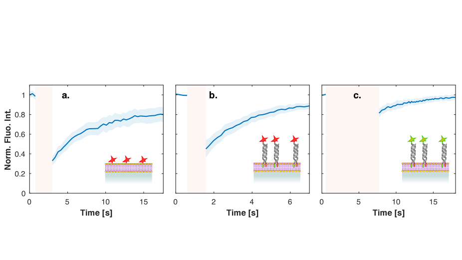
  Figure S1: FRAP experiments on substrate spheres. FRAP recovery curves as recorded on SLB-coated substrate spheres probing DHPE-TexasRed lipids (a), Cy5-functionalised DNA constructs (b) and Cy3-functionalised DNA constructs (c). Spheres in a were also decorated with non-fluorescent inert DNA constructs to accurately represent the experimental scenario. Spheres used for b and c lack the fluorescent lipids in their SLB. Sequences of the ssDNA components of the constructs used in b and c, which differ for the cholesterolised membrane-anchoring element, are summarised in Table S1. The shaded regions in all plots indicates the bleaching period, and its duration changes from sample to sample due to differences in the intensity of the relevant laser lines and the tendency to bleach of the different dyes. Curves are averaged over $\geq 6$ independent measurements performed on different spheres. The solid line and the shaded region surrounding it represent the mean and standard deviation of these measurements. In all cases, a clear recovery of the fluorescence is observed, demonstrating the lateral mobility of the tested probes. The timescales of the recovery are comparable with literature values for SLB on silica particles. Rinaldin et al. (2019)

  

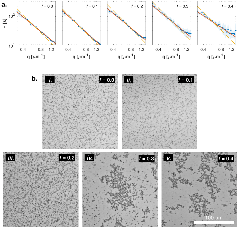
  Figure S2: Assessing particle aggregation visually and via DDM. a. Experimental values of the DDM relaxation time $\tau$ as a function of the wave vector $q$ recorded at the end of an aggregation experiment ($t=22$ hours) for all tested values of the fraction of linkers $f$. Points and the surrounding shaded region indicate, respectively, the mean and standard deviation calculated over 8 ROIs (2 fields of view). The solid line indicates the best power law fit $\tau\propto q^{-\alpha}$, while the dashed line the best Brownian fit $\tau=Dq^{-2}$. The latter is used to extract the effective diffusion coefficient $D$, shown in Fig. 2b and Fig. S3. Note that the datapoints deviate more significantly from the Brownian slope at large $f$, following the formation of branched aggregates with a complex dynamics. Cho et al. (2020). b. Bright field microscopy snapshots from the movies underlying the DDM data in panel a.

  

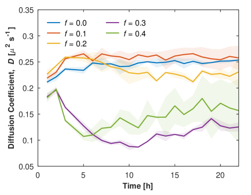
  Figure S3: Time evolution of the DDM effective diffusion coefficient for samples featuring both particles and substrate spheres. Note the similarity with the curves in Fig. 2b, indicating that the bulk phase behaviour of particles is unaffected by the substrate spheres, which have the only effect of regulating the deposition of some particles on their surface. The slight increase in $D$ observed at the beginning of the experiment in all sample may be a consequence of initial thermalisation.

  

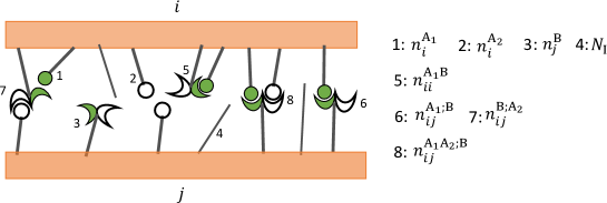
  Figure S4: Examples of intra-particle and inter-particle complexes. The planes represent the surface of particles $i$ and $j$ and carry reactive (${A_{1}}$, ${A_{2}}$, and ${B}$) and inert (I) linkers. $n^{\mathrm{X}}_{p}$ denotes the number of free linkers of type X ($\mathrm{X}={A_{1}}$, ${A_{2}}$, or ${B}$) tethered to particle $p$. Each complex is identified by its monomeric components and the planes to which they are anchored. For bridges, semicolumns separate the components tethered to particle $i$ from those tethered to particle $j$. Each particle carries $N_{I}$ inert constructs.

  

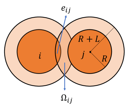
  Figure S5: Configurational volumes. Configurational volume excluded to a linker tethered to particle $j$ by the presence of particle $i$ ($e_{ij}$) and configurational volume available to interparticle bridges ($\Omega_{ij}$). The definitions of $e_{ij}$ and $\Omega_{ij}$ are given in Eq. 10. $R$ and $L$ denote the radius of the particles and the length of the linkers, respectively.

  

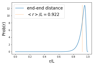
  Figure S6: Distribution of the end-to-end distance of a semiflexible rod with persistence length equal to twice the length of the rod $L$ (from Hamprecht and Kleinert (2005)). The dotted line nicks the average distance with a fixed end-to-end direction.

  

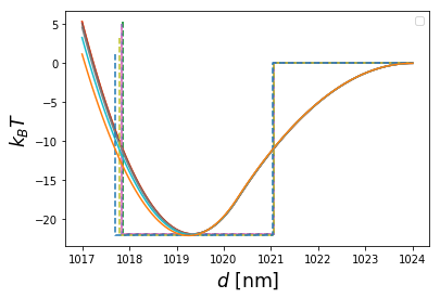
  Figure S7: Mapping free-energy profiles into square-well potentials. Full lines represent the multivalent free energies $\Delta F$ calculated using Eq. S2.2 while dashed lines the corresponding square-well potentials (see text). Different colors represent different temperatures ($T=20\,^{\circ}$C, $26\,^{\circ}$C, $T=33\,^{\circ}$C, $39\,^{\circ}$C, $45\,^{\circ}$C, and $50\,^{\circ}$C). Valency is equal to $z=4$ and the packing fraction to $\phi=28\%$.

  

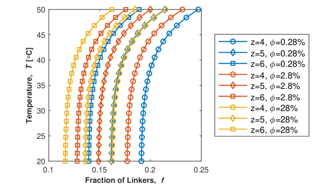
  Figure S8: Liquid-solid phase boundaries as calculated using the parameters in Table S2.