ISTD-GCN: Iterative Spatial-Temporal Diffusion Graph Convolutional Network for Traffic Speed Forecasting

Abstract.

Most of the existing algorithms for traffic speed forecasting split spatial features and temporal features to independent modules, and then associate information from both dimensions. However, features from spatial and temporal dimensions influence mutually, separated extractions isolate such dependencies, and might lead to inaccurate results. In this paper, we incorporate the perspective of information diffusion to model spatial features and temporal features synchronously. Intuitively, vertices not only diffuse information to the neighborhood but also to the subsequent state along with the temporal dimension. Therefore, we can model such heterogeneous spatial-temporal structures as a homogeneous process of diffusion. On this basis, we propose an Iterative Spatial-Temporal Diffusion Graph Convolutional Network (ISTD-GCN) to extract spatial and temporal features synchronously, thus dependencies between both dimensions can be better modeled. Experiments on two traffic datasets illustrate that our ISTD-GCN outperforms 10 baselines in traffic speed forecasting tasks. The source code is available at https://github.com/Anonymous.

1. Introduction

Spatial-temporal analysis has received increasing attention with the emergence of big data. In the real world, different types of data present dual attributes of spatial and temporal dimensions. Thus, spatial-temporal modeling is widely applied in various domains including urban computing (Yu et al., 2018; Li et al., 2018b; Wu et al., 2019a), climate science (Saha et al., 2010; Shi et al., 2015), neuroscience (Atluri et al., 2015), social media (Carney., 2016), etc. For instance, the traffic speed forecasting task is a typical application of spatial-temporal modeling since the traffic speed of specific locations not only depends on the traffic conditions nearby but also on the historical traffic information.

Considerable success has been made in traffic speed forecasting. The mainstream strategy is to incorporate convolutional models to handle spatial features (including Convolutional Neural Networks (Ma, 2017; Zhang et al., 2017; Xian et al., 2018) and Graph Convolutional Neural Networks (Yu et al., 2018; Li et al., 2018b; Wu et al., 2019a; Guo et al., 2019)), while sequential models (including Recurrent Neural Networks (Li et al., 2018b; Wang et al., 2018), Temporal Convolutional Neural Networks (Yu et al., 2018; Wu et al., 2019a) and Attention Mechanism (Guo et al., 2019)) for temporal features. DCRNN (Li et al., 2018b) and Graph WaveNet (Wu et al., 2019a) firstly adopt an information diffusion model to capture spatial information, which has been proved to be a well simulation of traffic flow in the real world. The perspective of information diffusion for spatial features modeling achieves great success.

Nevertheless, a potential pitfall should be noticed: most of the existing models extract spatial and temporal information separately, and then associate information from both dimensions by specific methods (concatenation, linear transformation, attention mechanism, etc.). However, in spatial-temporal data, spatial features and temporal features interact mutually, separated extraction might lead to the loss of dependencies, and then produce inaccurate modeling.

For removing the weaknesses, we proposed a model called ISTD-GCN (Iterative Spatial-Temporal Diffusion Graph Convolutional Network) to capture spatial and temporal features synchronously. Explicitly, we model traffic flow as a process of information diffusion. Different from DCRNN (Li et al., 2018b) and Graph WaveNet (Wu et al., 2019a), in our model, the process of information diffusion not only happens in the spatial dimension but also in the temporal dimension simultaneously. Vertices diffuse information to the neighborhood but also to the next state along with the temporal dimension. From this perspective, we can capture spatial features and temporal features simultaneously in a unified process of diffusion graph convolution. The pattern of spatial-temporal synchronous diffusion is shown in Figure 1.

The main contributions of our work are as follows:

• We incorporate the perspective of information diffusion to model spatial features and temporal features synchronously in spatial-temporal data. Therefore, the dependencies between features from both dimensions have been greatly remained, and more accurate modeling can be generated.

• Based on the perspective of spatial-temporal synchronous diffusion, we propose a joint framework ISTD-GCN (Iterative Spatial-Temporal Diffusion Graph Convolutional Network) for modeling traffic speed forecasting task. In ISTD-GCN, we adopts three novel key components for better simulation of spatial-temporal information diffusion and leads to more accurate modeling.

• We conduct several experiments with two real-world traffic speed datasets. The experimental results demonstrate that our proposed model outperforms other comparison methods.

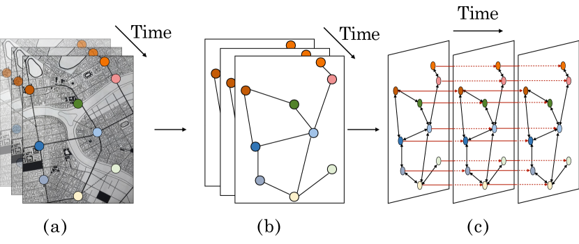
Figure 1. (a) illustrates the raw data collected from the original urban maps. The colored points represent points in the city to record traffic speed. The recorded speed will changes with time, while the positions of the colored points are constant. (b) shows the original urban map sequence is abstracted as a graph sequence, where the colored points are denoted as vertices in a graph, and the edges encode the pair-wise relationship among colored points in the original urban maps. (c) shows the directions of information diffusion in our model. The red lines represent the the diffusion along with the temporal dimension, while the black lines represent the diffusion of the spatial dimension. Note that the diffusion along with the temporal dimension is uni-directional.

2. Preliminary

2.1. Traffic Speed Forecasting Problem

The urban road network can be abstracted as a graph, which is represented as $\mathcal{G}=(\mathcal{V},\mathcal{E},W)$, where $\mathcal{V}$ is the set of vertices in graph $\mathcal{G}$ with $|\mathcal{V}|=n$, while $\mathcal{E}$ represents the set of edges. $W\in{\mathbb{R}^{n\times{n}}}$ denotes the weighted adjacency matrix that is derived from the graph $\mathcal{G}$. Entry $W_{ij}$ in matrix $W$ is used to describe the proximity between vertex $i$ and vertex $j$. The detailed construction of the weighted adjacency matrix $W$ is introduced in section 4.1. Note that the topology of graph $\mathcal{G}$ is constant along with the temporal dimension, which means that the weighted adjacency matrix $W$ is also constant. The tensor of dynamic features $X\in{\mathbb{R}^{T\times{n}\times{d}}}$ is the recorded historical observations, where $T$ represents the number of historical time steps, and $d$ denotes the dimension of features. $X^{(t)}$ represents the features of vertices of $\mathcal{G}$ at time step $t$, $\mathcal{G}^{(t)}=(\mathcal{G},X^{(t)})$ is the snapshot of graph $\mathcal{G}$ at time step $t$. The formal definition of traffic speed forecasting problem is to find a mapping function $f(.)$, such that we can infer the snapshots of graph $\mathcal{G}$ in the future $H$ snapshots according to $T$ historical observations:

(1) $$f(\mathbb{G}^{(t_{0}:t_{T-1})})=\mathbb{G}^{(t_{T}:t_{T+H-1})},$$

where $\mathbb{G}^{(t_{0}:t_{T-1})}=(\mathcal{G}^{(t_{0})},\mathcal{G}^{(t_{1})},\cdots,\mathcal{G}^{(t_{T-1})})$ represents the $T$ historical observed snapshots, while $\mathbb{G}^{(t_{T}:t_{T+H-1})}=(\mathcal{G}^{(t_{T})},\mathcal{G}^{(t_{T+1})},\cdots,\\ \mathcal{G}^{(t_{T+H-1})})$ denotes the $H$ future predicted snapshots.

2.2. Diffusion Graph Convolutional Neural Networks

Graph neural networks archive great success in handling spatial dependencies in non-Euclidean structures. In our model, we refer to the Graph Convolutional Neural Network proposed by Kipf et al. (Kipf and Welling., 2017) as the vanilla GCN. Graph Convolutional Layers in the vanilla GCN are defined as:

(2) $$X^{(l+1)}=\sigma(\tilde{D}^{-\frac{1}{2}}\tilde{W}\tilde{D}^{-\frac{1}{2}}\Theta^{(l)}X^{(l)}),$$

where $X^{(l+1)}$ and $X^{(l)}$ are the output and input for layer $l$, respectively. $\tilde{W}=W+I_{n}$ is the weighted adjacency matrix with self-connections, where $W$ denotes the weighted adjacency matrix and $I_{n}$ is an identity matrix. $\tilde{D}_{ii}=\sum_{j}\tilde{W}_{ij}$ is the degree matrix of $\tilde{W}$. $\Theta^{(l)}$ is the trainable parameters and $\sigma$ is the activation function. The item $\tilde{D}^{-\frac{1}{2}}\tilde{W}\tilde{D}^{-\frac{1}{2}}$ denotes the symmetric normalization of the weighted adjacency matrix.

Li et al. (Li et al., 2018b) proposed a diffusion graph convolutional neural network (diffusion GCN for short) for better suiting the nature of traffic flow. Specifically, Teng et al. (Teng, 2016) had proved that the diffusion process of information on graph $\mathcal{G}$ can be formulated as a process of random work with restart probability $\alpha\in{[0,1]}$ and transition matrix $(\tilde{D}^{-1}\tilde{W})$. The stationary distribution of the diffusion process can be represented as a weighted combination of infinite random walks on the graph and be calculated in closed form:

(3) $$\mathcal{P}=\sum^{\infty}_{k=0}\alpha(1-\alpha)^{k}(\tilde{D}^{-1}\tilde{W})^{k},$$

where $\mathcal{P}\in{\mathbb{R}^{n\times{n}}}$ denotes the stationary distribution of the Markov process of diffusion. In DCRNN (Li et al., 2018b), the authors used a finite K-step truncation of the diffusion process and assigned a trainable weight to each step. Therefore, a step of uni-directional process of information diffusion in DCRNN can be rewritten as:

(4) $$X^{(l+1)}=\sigma(\tilde{D}^{-1}\tilde{W}\Theta^{(l)}X^{(l)}),$$

Note that the only difference between Equation (2) and Equation (4) in the form is the approach of normalization, nevertheless, there exists fundamental differences on the meanings. In Equation (2), the item $\tilde{D}^{-\frac{1}{2}}\tilde{W}\tilde{D}^{-\frac{1}{2}}$ denotes the symmetric normalization of the weighted adjacency matrix $\tilde{W}$, while the item $\tilde{D}^{-1}\tilde{W}$ in Equation (4) denotes the transition matrix in Markov process of information diffusion.

3. Methodology

In this section, we formally describe our model: ISTD-GCN. The core idea behind our model is that vertices diffuse message not only to the neighborhood but also to the subsequent state along with the temporal dimension. Specifically, there are three key components in our model ISTD-GCN: the Heterogeneous Spatial-Temporal Graph, the Two-Step Convolution, and the Iterative Strategy.

3.1. Heterogeneous Spatial-Temporal Graph

The Heterogeneous Spatial-Temporal Graph (HSTG for short) performs a key role in our model. Spatial-temporal data is inherently heterogeneous since features from both dimensions carry different types of information. Nevertheless, from the perspective of information diffusion, the process of diffusion in both dimensions share the homogeneous pattern. The only difference between the processes of diffusion on both dimensions is the weights, which control the intensity of signals in the information that to be diffused. Therefore, we can connect adjacent snapshots by generating directed edges to its subsequent state along with the temporal dimension. The illustration of HSTG that is generated by adjacent 3 snapshots is shown in Figure 2.

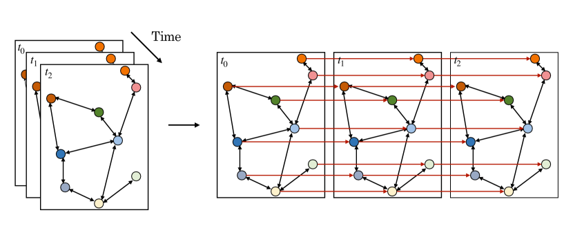
Figure 2. Heterogeneous Spatial-Temporal Graph (HSTG). Black arrows represent bi-directional information diffusion in the spatial dimension, while red arrows represent the uni-directional diffusion in the temporal dimension.

Formally, we can obtain a sequence of snapshots of graph $\mathcal{G}$ according to $T$ historical observations: $\mathbb{G}^{(t_{0}:t_{T-1})}=(\mathcal{G}^{(t_{0})},\mathcal{G}^{(t_{1})},\cdots,\\ \mathcal{G}^{(t_{T-1})})$. On this basis, we can select arbitrary continuous sub-sequence $\mathbb{G}^{(t^{\prime}:t^{\prime}+m-1)}=(\mathcal{G}^{(t^{\prime})},\mathcal{G}^{(t^{\prime}+1)},\cdots,\mathcal{G}^{(t^{\prime}+m-1)})$ in $\mathbb{G}^{(t_{0}:t_{T-1})}$ with $m$ snapshots, where $t^{\prime}\geq t_{0}$ and $t^{\prime}+m-1\leq t_{T-1}$. Therefore, we can connect all snapshots in $\mathbb{G}^{(t^{\prime}:t^{\prime}+m-1)}$ and generate a HSTG, the HSTG is denoted as $\mathcal{G}_{(H)}=(\mathcal{V}_{(H)},\mathcal{E}_{(H)},W_{(H)})$ with corresponding features $X_{(H)}$, where $\mathcal{V}_{(H)}$ and $\mathcal{E}_{(H)}$ denote vertices and edges in the HSTG, respectively, while $W_{(H)}$ is the weighted adjacency matrix of the HSTG. Thus, we can obtain a new graph called Heterogeneous Spatial-Temporal Graph (HSTG) by the means of connection of snapshots. The weighted adjacency matrix $W_{(H)}$ of the HSTG is defined as:

(5) $$W_{(H)}=\begin{pmatrix}W&C&0&\cdots&0&0&0\\ 0&W&C&\cdots&0&0&0\\ \vdots&\vdots&\vdots&\ddots&\vdots&\vdots&\vdots\\ 0&0&0&\cdots&W&C&0\\ 0&0&0&\cdots&0&W&C\\ 0&0&0&\cdots&0&0&W\\ \end{pmatrix}\in{\mathbb{R}^{mn\times{mn}}},$$

where $C$ denotes an matrix consists of the generated edges that connecting all snapshots.

Analogously, the features of corresponding snapshots should also be stacked:

(6) $$X_{(H)}=STACK(X^{(t^{\prime})},X^{(t^{\prime}+1)},\cdots,X^{(t^{\prime}+m-1)})\in\mathbb{R}^{m\times{n\times{d}}},$$

where $STACK(.)$ denotes the operation of stacking.

Intuitively, we can generate edges to connect the corresponding vertices between different graph snapshots, the generated edges should be directed since time series is uni-directional, which can be reflected by the upper triangular adjacency matrix $W_{(H)}$. In addition, The weights of these generated directed edges can be arbitrary since the intensity of diffused information can be also adjusted by the auto-learned parameters. In our setting, for simplification, we set the weights of these generated directed edges as 1. In another word, we specify an identity matrix to connect adjacent snapshots, i.e., $C=I_{n}$ in Equation (5), where $I_{n}$ denotes an identity matrix. Meanwhile, the original undirected graph $\mathcal{G}$ at each snapshots $\mathcal{G}^{(t)}=(\mathcal{G},X^{(t)})$ is also transformed into a directed graph, in which the original undirected edges are transformed into bi-directional edges. From the weighted adjacency matrix of HSTG $W_{(H)}$ we can also easily obtain the corresponding degree matrix $D_{(H)}$, where $D_{(H)ii}=\sum_{j}W_{(H)ij}$, and its inverse matrix $D_{(H)}^{-1}$.

Therefore, the preconditions for performing diffusion GCN described as Equation (4) on HSTG is obtained.

3.2. Two-Step Convolution

We can perform diffusion graph convolution on the HSTG $\mathcal{G}_{(H)}$ to simultaneously extract features from the spatial dimension and the temporal dimension as following form:

(7) $$\hat{X}=\sigma{(D_{(H)}^{-1}W_{(H)}\Theta X_{(H)})},$$

where $\hat{X}$ denotes the output of the layer.

As we mentioned above, the process of information diffusion in both dimensions is homogeneous. Nevertheless, features in both dimensions are not homogeneous since features in different dimensions carry diffenrent types of information. In other words, spatial features and temporal features not in the same semantic space. In our model, however, is not able to distinguish which semantic space the features come from, since features from both dimensions share the homogeneous and synchronous process of extraction. This issue might lead to excessive confusion of features from both dimensions and cause performance degration.

For handling the problem, we propose a process of two-step diffusion graph convolution (two-step convolution for short) to force the model distinguish features from different dimensions under the same process of information diffusion. Specifically, we perform convolution on each snapshot before convolution on HSTG, the purpose is to add simple marks for information from different dimensions for identification. In a nutshell, in each step of our proposed two-step diffusion, we perform information diffusion once in the temporal dimension, while twice in the spatial dimension. Therefore, the model can easily distinguish features from both dimensions. Formally, we disconnect the edges among different snapshots that diffuse the temporal features in HSTG, and generate a new graph called non-Heterogeneous Spatial Temporal Graph (NHSTG for short) with $m$ connected components, which is denoted as $\mathcal{G}_{(NH)}=(\mathcal{V}_{(NH)},\mathcal{E}_{(NH)},W_{(NH)})$. The weighted adjacency matrix $W_{(NH)}$ for NHSTG is defined as:

(8) $$W_{(NH)}=\begin{pmatrix}W&0&\cdots&0&0\\ 0&W&\cdots&0&0\\ \vdots&\vdots&\ddots&\vdots&\vdots\\ 0&0&\cdots&W&0\\ 0&0&\cdots&0&W\\ \end{pmatrix}\in{\mathbb{R}^{mn\times{mn}}},$$

analogously, $D_{(NH)ii}=\sum_{j}W_{(NH)ij}$ denotes the degree matrix of $\mathcal{G}_{(NH)}$. The detailed process of the two-step convolutional layer is shown in Figure 3.

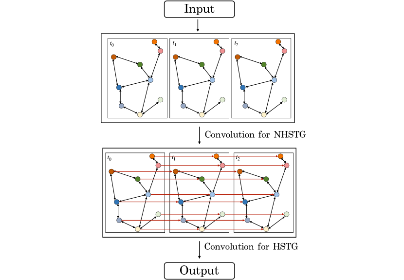
Figure 3. Two-Step Convolutional Layer.

We stack several two-step convolutional layers for better performance to generate a spatial-temporal synchronous convolutional block (STSC block for short) in our model. Formally, the naive process of feedforward of our STSC block is defined as:

(9) $$\hat{X}=\sum_{k=1}^{K}(\sigma((\Theta_{k,1}D_{(NH)}^{-1}W_{(NH)})^{k}X_{(NH)})+\sigma((\Theta_{k,2}D_{(H)}^{-1}W_{(H)})^{k}X_{(H)})),$$

where $K$ denotes the number of stacked two-step convolutional layers, i.e., the receptive field of graph convolutional neural networks, $\Theta_{k,1}$ and $\Theta_{k,2}$ are trainable parameters, while $X_{(NH)}$ and $X_{(H)}$ are input features of convolution on NHSTG and HSTG, respectively.

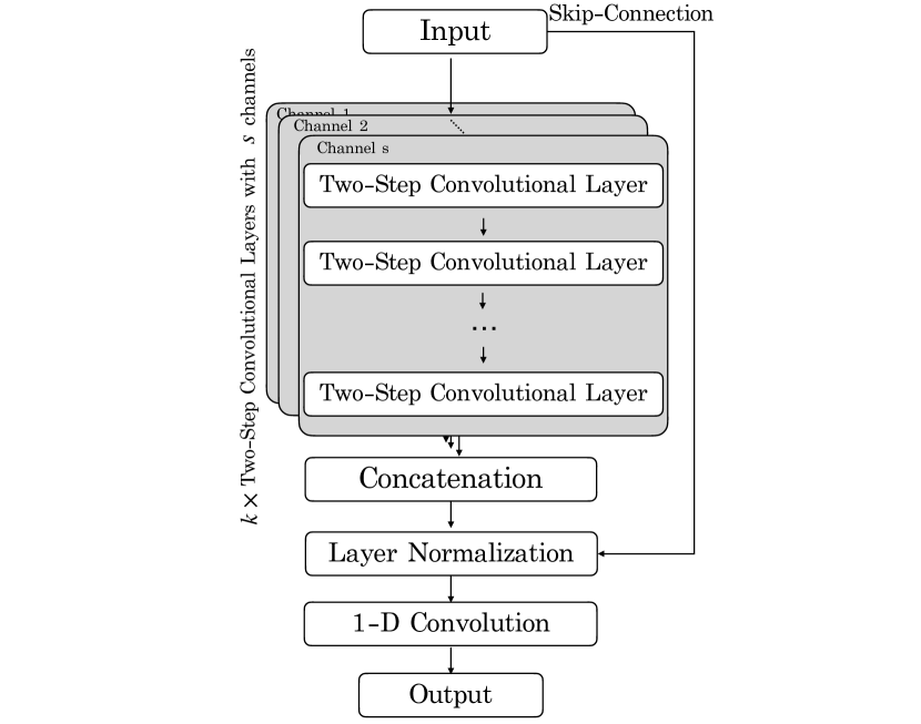
Figure 4. Spatial-Temporal Synchronous Convolutional Block (STSC Block).

The primary purpose of the two-step convolution is to diffuse information instead of non-linear transformation. Inspired by SGC (Wu et al., 2019b), we removed all non-linear activation layers in the process of convolution for simplification. For ensuring the stability of representations in hidden layers, we add a layer normalization (Ba et al., 2016) for the output of STSC blocks. We also add skip connection for residual learning to obtain more efficient training (He et al., 2015) and alleviate over-smoothing (Li et al., 2018a). In addition, the vertices in the NHSTG are the same as the HSTG since we generate the NHSTG by only removing edges. Therefore, $\mathcal{V}_{(NH)}=\mathcal{V}_{(H)}$, corresponding features of the NHSTG are also the same as the features of the HSTG, i.e., $X_{(NH)}=X_{(H)}$. Thus, the propagation rules of our STSC blocks are formally defined as:

(10) $$\hat{X}=LN(\sum_{k=1}^{K}(\Theta_{k,1}(D_{(NH)}^{-1}W_{(NH)})^{k}+\Theta_{k,2}(D_{(H)}^{-1}W_{(H)})^{k})X_{(H)}+X_{(H)}),$$

where $LN(.)$ represents layer normalization.

Note that the output $\hat{X}\in{\mathbb{R}^{m\times{n}\times{d}}}$ contains features of all vertices in HSTG after STSC block. We have to compress the output as a new compressed snapshot since we need to participate in the subsequent operations. Therefore, we adopt an 1-D convolutional layer to compress the output information. Thus, we obtain the compressed feature $\hat{X}\in{\mathbb{R}^{n\times{d}}}$ from the output of STSC block after an operation of 1-D convolution. The illustration of a STSC block is shown in Figure 4.

In addition, inspired by the successful application of multi-channel in classical convolutional neural networks (Krizhevsky et al., 2012), we adopt several diffenrent graph convolutaion kernels to extract information in different sub-spaces of representations. The outputs of each channel are concatenated:

(11) $$\hat{X}=\big{|}\big{|}_{i\in{s}}\hat{X}_{i},$$

where $\big{|}\big{|}$ denotes the operation of concatenation for features, $\hat{X}_{i}\in{\mathbb{R}^{n\times{d}}}$ denotes the output of the $i$-th STSC block, $\hat{X}\in{\mathbb{R}^{n\times{sd}}}$ represents the final output of our multi-channel graph convolution, and $s$ is the number of channels. Therefore, we obtain the output $\hat{X}\in{\mathbb{R}^{n\times{sd}}}$, we adopt a linear transformation to reduce the dimension of $\hat{X}$. Finally, the output of STSC block is denoted as $\hat{X}\in{\mathbb{R}^{n\times{d}}}$.

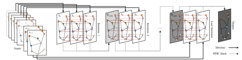
Figure 5. The illustration of Iterative Spatial-Temporal Diffusion Graph Convolution. The darker color of graphs represent the compressed snapshots that store and comporess more information in previous snapshots.

3.3. Iterative Strategy

Connecting all snapshots to generate larger HSTG and NHSTG in historical observations $\mathbb{G}^{(t_{0}:t{T-1})}$ is not an optimal strategy in spatial-temporal data for three reasons:

1. Overfitting. Connecting all snapshots yields a larger trainable parameter matrix as the graph convolutional kernel, which carries more parameters and leads to an unstable convergence. A larger parameter matrix exacerbates the complexity of our model, and might lead to overfitting.

2. The loss of local dependencies. Intuitively, in the time series, a snapshot is mainly affected by its adjacent snapshots, and also mainly affects adjacent snapshots, we refer to this property the local dependencies in the temporal dimension. In our model, the process of information diffusion among adjacent snapshots shares the similar pattern. A lager graph convolutional kernel that caused by connecting all snapshots might ignore such dependencies.

3. The phenomenon of information bottleneck (Tishby and Zaslavsky., 2015). The structure of our model can be regarded as a variant of Encoder-Decoder architecture (Bahdanau et al., 2015) (detailed illustration in section 3.4). Specifically, in the part of the encoder, we encode information in $T$ historical observations into one snapshot, and the ratio of compression is $\frac{T-1}{T}$, i.e., the loss of information due to the process of one-time encoding. As $T$ increases, the loss of information in the process of one-time encoding become unacceptable.

For handling these issues, motivated by previous works that successfully applied 1-D convolutional neural networks with smaller convolutional kernels on sequential data (Kalchbrenner et al., 2014; Kim., 2014), we design a strategy of iteration to adapt our model. The detailed process of iterative strategy is shown in Figure 5.

Specifically, in the iteration 1, we select the adjacent $m(m<T)$ snapshots to generate a HSTG (denoted as $\mathcal{G}_{(H)}$) and a NHSTG (denoted as $\mathcal{G}_{(NH)}$), then we feed the STSC block on the generated HSTG $\mathcal{G}_{(H)}$ and NHSTG $\mathcal{G}_{(NH)}$ to perform two-step convolution according to Equation (10). Therefore, we can obtain a new snapshot $\mathcal{G}_{com}$ that compresses the information from the selected adjacent $m$ snapshots:

(12) $$\mathcal{G}_{com}=(\mathcal{G},X_{com}^{(t_{0},t_{1},\cdots,t_{m-1})}),$$

where $X_{com}^{(t_{0},t_{1},\cdots,t_{m-1})}\in{\mathbb{R}^{1\times{n\times{d}}}}$ denotes the compressed features that store the information from $X^{(t_{0})}$ to $X^{(t_{m-1})}$. The topology of $\mathcal{G}_{com}$ equals $\mathcal{G}$. Then, the compressed snapshot $\mathcal{G}_{com}$ is further connected with the following $(m-1)$ snapshots and perform the same operation iteratively. The iteration is processing until the end of the sequence of historical observed snapshots $\mathbb{G}^{(t_{0}:t_{T-1})}$.

Thus, we can solve problems caused by connecting all snapshots. Simple illustrations are as following:

1. Solution for overfitting. The main reason for overfitting is excessive trainable parameters lead to extra complexity of model. In the strategy of iteration, the number of entries in graph convolutional kernel is $m^{2}n^{2}$, where $m$ denotes the number of connected adjacent snapshots, $n$ is the number of vertices. If we connect all snapshots in the historical observations, the number will increases to $T^{2}n^{2}$. Obviously, $m^{2}n^{2}\textless T^{2}n^{2}$ since $m\textless T$. Lower number of trainable parameters leads to lower complexity, which can prevent overfitting effectively.

2. Solution for the loss of local dependencies. Abundant different applications of Convolutional Neural Networks in images (Krizhevsky et al., 2012; Howard et al., 2017; Sandler et al., 2018) and sequential data (Kalchbrenner et al., 2014; Kim., 2014; Wu et al., 2019a; Yu et al., 2018; van den Oord et al., 2016) have proved that smaller convolutional kernels can better handle local dependencies, which larger convolutional kernels more adapt at extract global features.

3. Solution for the phenomenon of information bottleneck. the phenomenon of information bottleneck is caused by excessive information compression in one-time, which might lead to serious loss of information. Specifically, the ratio of compression is $\frac{T-1}{T}$ without the strategy of iteration. If we incorporate the strategy of iteration, the features will undergo multiple compressions, and the ratio of compression in each of the process is $\frac{m-1}{m}$. Obviously, $\frac{T-1}{T}>\frac{m-1}{m}$ because $m<T$. Therefore, in each compression, the ratio of compression decreases, which means that more useful information is remained and fewer information is lost. Thus, after multiple processes of compression with lower ratio of compression, we can alleviate the phenomenon of information bottleneck, compared with one time with higher ratio of compression.

3.4. Overall Architecture

In this subsection, we make a comprehensive description of our model ISTD-GCN. The overall illustration of the model is shown in Figure 6. In general, we employ the Encoder-Decoder architecture (Bahdanau et al., 2015).

Encoder: As shown in the Figure 6, the encoder is composed of the part (a), the part (b) and the (c). Specifically, part (a) is the input sequence of snapshots according to $T$ historical observations: $\mathbb{G}^{(t_{0}:t_{T-1})}=(\mathcal{G}^{(t_{0})},\mathcal{G}^{(t_{1})},\cdots,\mathcal{G}^{(t_{T-1})})$. The sequence $\mathbb{G}^{(t_{0}:t_{T-1})}$ is fed into the part (b) and perform Iterative Spatial-Temporal Graph Diffusion Convolution, which is described detailedly in subsection 3.2 and subsection 3.3. Specifically, the diffusion graph convolution is performed as Equation (10) in each iteration, the iteration is repeated until the end of the sequence of historical observed snapshots $\mathbb{G}^{(t_{0}:t_{T-1})}$. The output of the Iterative Spatial-Temporal Graph Diffusion Convolution, and shown in part (c). The new compressed snapshot that shown in part (c) compresses and stores all information of the input sequence of snapshots, which is denoted as $\mathcal{G}_{enc}=(\mathcal{G},X_{enc})$, where $X_{enc}\in\mathbb{R}^{1\times{n\times{d}}}$.

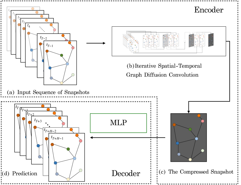
Figure 6. The overview of ISTD-GCN.

Decoder: The decoder is simply but effective. Inspired by Wu et al. (Wu et al., 2019a), for eliminating the accumulative error caused by RNN-based decoders, we adopt a Multilayer Perceptron (MLP) to parallelly decode the information at each position. Specifically, the features $X_{enc}\in\mathbb{R}^{1\times{n\times{d}}}$ are transformed into $X_{dec}\in\mathbb{R}^{H\times{n\times{d}}}$ by the MLP. Therefore, we can obtain a sequence that composed of $H$ snapshots $\mathbb{G}^{(t_{T}:t_{T+H-1})}=(\mathcal{G}^{(t_{T})},\mathcal{G}^{(t_{T+1})},\cdots,\mathcal{G}^{(t_{T+H-1})})=((\mathcal{G},X^{(0)}_{dec}),(\mathcal{G},X^{(1)}_{dec}),\cdots,(\mathcal{G},X^{(H-1)}_{dec}))$ to predict $H$ future conditions, shown as part (d).

Detailed process of ISTD-GCN is shown as Algorithm 1.

Data: the number of connected snapshots $m$, the sequence of $T$ historical snapshots $\mathbb{G}^{(t_{0}:t_{T-1})}=(\mathcal{G}^{(t_{0})},\mathcal{G}^{(t_{1})},\cdots,\mathcal{G}^{(t_{T-1})})$.

Result: the predicted $H$ snapshots $\mathbb{G}^{(t_{T}:t_{T+H-1})}=(\mathcal{G}^{(t_{T})},\mathcal{G}^{(t_{T+1})},\cdots,\mathcal{G}^{(t_{T+H-1})})$.

1

2while not at the end of the sequence $\mathbb{G}^{(t_{0}:t_{T-1})}$ do

3       if is the first iteration then

4             select continuous sub-sequence with $m$ snapshots from the beginning of $\mathbb{G}^{(t_{0}:t_{T-1})}$ as $\mathbb{G}_{s}=\mathbb{G}^{(t_{0}:t_{m-1})}=(\mathcal{G}^{(t_{0})},\mathcal{G}^{(t_{1})},\cdots,\mathcal{G}^{(t_{m-1})})$;

5            

6      else

7             the current index of iteration is $k$;

8             select continuous with following $m-1$ snapshots, and concatenate $\mathcal{G}_{com}$ with the selected sub-sequence as $\mathbb{G}_{s}=(\mathcal{G}_{com},\mathcal{G}^{(t_{k(m-1)+2})},\cdots,\mathcal{G}^{(t_{k(m+1)-1})})$;

9            

10       end if

11      Generate corresponding HSTG $\mathcal{G}_{(H)}=(\mathcal{V}_{(H)},\mathcal{E}_{(H)},W_{(H)})$ and NHSTG $\mathcal{G}_{(NH)}=(\mathcal{V}_{(NH)},\mathcal{E}_{(NH)},W_{(NH)})$ accoding to $\mathbb{G}_{s}$.;

12       Perform the Two-Step Convolution as Equation (10).;

13       Generate the compressed snapshot $\mathcal{G}_{com}$.

14 end while

15$\mathbb{G}^{(t_{T}:t_{T+H-1})}=MLP(\mathcal{G}_{com})=(\mathcal{G}^{(t_{T})},\mathcal{G}^{(t_{T+1})},\cdots,\mathcal{G}^{(t_{T+H-1})})$ ;

16

Algorithm 1 Iterative diffusion graph convolution

3.5. Objective Function

We incorporate Mean Absolute Error(MAE) as the loss function of ISTD-GCN. Furthermore, for avoiding overfitting, we adopt L2 regularization.

(13) $$L=\frac{1}{HND}\sum_{t=t_{T}}^{t_{T}+H-1}\sum_{n=1}^{N}\sum_{d=1}^{D}|\hat{X}_{nd}^{(t)}-X_{nd}^{(t)}|+\lambda\left\|\Theta\right\|_{2},$$

where $H$,$N$,$D$ represent the number of predicted snapshots, the number of vertices in $\mathcal{G}$ and the dimension of features, respectively. $\lambda$ is the coefficient of the L2 regularization and $\Theta$ denotes all trainable parameters in our model.

4. Experiments

4.1. Datasets

To illustrate the effect of our proposed ISTD-GCN, we process experiments on two real-world traffic datasets METR-LA and PEMS-BAY. The necessary information of both datasets is shown in Table 2.

METR-LA dataset records four months of traffic flow speed information on 207 sensors on the highways of Los Angeles.

PEMS-BAY dataset records six months of traffic flow speed information on 325 sensors in the Bay area.

For the fairness of the comparison, we adopt the same strategy of data preprocessing with previous works (Li et al., 2018b; Wu et al., 2019a). Specifically, both datasets aggregate records into 5-minute interval, and 288 snapshots per day. In addition, we adopt the same strategy of using Gaussian kernel (Shuman et al., 2012) to construct the spatial weighted adjacency matrix:

(14) $$W_{ij}=\begin{cases}\exp{(-\frac{d_{ij}^{2}}{\sigma^{2}})}&d_{ij}\leq\epsilon\\ 0&d_{ij}>\epsilon\end{cases},$$

where $d_{ij}$ denotes the real geographic distance between sensor $i$ and sensor $j$, $\sigma$ is the standard deviation of distances, and $\epsilon$ is a threshold. The greater $W_{ij}$ is, the more relevant vertex $i$ and vertex $j$ is. Both settings of $\sigma$ and $\epsilon$ are the same as in Graph Wavenet (Wu et al., 2019a). For the stability of distribution, Z-score normalization is also applied to the input in order to convert the data distribution to a normal distribution. Z-score is calculated as:

(15) $$Z=\frac{X-\bar{X}}{S},$$

where $X$ denotes the sample to be processed, $\bar{X}$ denotes the mean of samples and $S$ is the standard deviation of the samples.

Table 1. Basic information of datasets

Dataset	#Vertices	#Edges	#snapshots
METR-LA	207	1515	34272
PEMS-BAY	325	2368	52116

4.2. Experimental Description and Metrics

In our experiments, we adopt 12 snapshots (60 minutes) as historical observations and predict traffic speed conditions in future 3 snapshots (15 minutes), 6 snapshots (30 minutes) and 12 snapshots (60 minutes), respectively. We evaluate the performance by three metrics: Mean Absolute Error (MAE), Root Mean Squared Errors (RMSE), and Mean Absolute Percentage Errors (MAPE). These metrics are calculated as:

(16) $$MAE(\hat{X},X)=\frac{1}{HND}\sum_{t=t_{T}}^{t_{T}+H-1}\sum_{n=1}^{N}\sum_{d=1}^{D}|\hat{X}_{nd}^{(t)}-X_{nd}^{(t)}|,$$

(17) $$RMSE(\hat{X},X)=\frac{1}{HND}\sum_{t=t_{T}}^{t_{T}+H-1}\sum_{n=1}^{N}\sum_{d=1}^{D}\sqrt{(\hat{X}_{nd}^{(t)}-X_{nd}^{(t)})^{2}},$$

(18) $$MAPE(\hat{X},X)=\frac{1}{HND}\sum_{t=t_{T}}^{t_{T}+H-1}\sum_{n=1}^{N}\sum_{d=1}^{D}\frac{|\hat{X}_{nd}^{(t)}-X_{nd}^{(t)}|}{X_{nd}^{(t)}+\delta},$$

where $\delta$ denotes a tiny shift to prevent the denominator equals zero.

We adopt the same proportion with DCRNN (Li et al., 2018b) and Graph WaveNet (Wu et al., 2019a) to generate training set (60%), validation set (20%) and test set (20%). We implement our model by PyTorch, and the key hyper-parameters of our model is shown in Table 2.

Table 2. Hyper-parameters Instruction

Hyper-parameter	Symbol	Value
The number of layers for two-step convolution	$K$	5
Number of connected adjacent snapshots	$m$	2
Number of convolutional channels	$s$	8
Dimension of hidden layers	$d$	256
Learning rate	-	0.0005

4.3. Baselines

We compared our proposed ISTD-GCN with the following algorithms:

• HA. Historical Average.

• ARIMA. Auto-Regressive Integrated Moving Average model with Kalman filter.

• VAR. Vector Auto Regression (Hamilton., 1994).

• SVR. Support Vector Regression which uses linear support vector machine for the regression task. (H. et al., 1997)

• FNN. Feedforward Neural Network.

• FC-LSTM. Recurrent Neural Network with Fully Connected LSTM hidden units (Sutskever et al., 2014).

• WaveNet. An 1-D convolutional neural network based archietecture for sequence data (van den Oord et al., 2016).

• DCRNN. Diffusion Convolutional Recurrent Neural Network. One of the pioneers that incorporating graph neural networks to forecast traffic speed (Li et al., 2018b).

• STGCN. Spatial-Temporal Graph Convolution Network. A combination of graph convolutional network and 1-D convolutional network (Yu et al., 2018).

• GraphWavenet. A combination of graph convolution and dilated casual convolution (Wu et al., 2019a).

4.4. Performance Comparison

In this subsection, we process detailed performance comparison with aforementioned baselines on dataset METR-LA and PEMS-BAY. The results of comparison on both datasets are shown in Table 3 and Table 4, respectively. From the performance comparison, it could be concluded that our proposed ISTD-GCN surpasses other baselines in most of the metrics. Especially, our algorithm outperforms other competitive algorithms in long-term forecasting tasks, since the parallel decoding eliminates the accumulative errors. At the same time, accuracy is maintained since the last compressed output of the encoder compresses all valuable information in previous snapshots.

4.5. Ablation Studies

We also perform ablation studies to illustrate that three key components in ISTD-GCN is effective. The detailed results of ablation studies on both datasets are also shown in the of Table 3 and Table 4, respectively.

Specifically, for validating the effect of Spatial-Temporal Synchronous Diffusion, we delete the component of Heterogeneous Spatial-Temporal Graph (HSTG) by removing the process of information diffusion in the temporal dimension. Analogously, we delete the process of convolution on the non-Heterogeneous Spatial-Temporal Graph (NHSTG) in the Two-Step Convolution to illustrate the effect of Two-Step Convolution. Finally, we set the number of connected adjacent snapshots $m$ equals the number of historical observations $T$, i.e., $m=T$. Therefore, our algorithm degenerate as a non-iterative algorithm.

Table 3. Performance comparison and ablation studies on METR-LA

Model/Condition	15 min			30 min			60 min
	MAE	RMSE	MAPE(%)	MAE	RMSE	MAPE(%)	MAE	RMSE	MAPE(%)
HA	4.16	7.80	13.00	4.16	7.80	13.00	4.16	7.80	13.00
ARIMA	3.99	8.21	9.60	5.15	10.45	12.70	6.90	13.23	17.40
VAR	4.42	7.89	10.20	5.41	9.13	12.70	6.51	10.11	15.80
SVR	3.99	8.45	9.30	5.05	10.87	12.10	6.72	13.76	16.70
FNN	3.99	7.94	9.90	4.23	8.17	12.90	4.49	8.69	14.00
FC-LSTM	3.44	6.30	9.60	3.77	7.32	10.90	4.37	8.69	13.20
WaveNet	2.99	5.89	8.04	3.59	7.28	10.25	4.45	8.93	13.62
DCRNN	2.77	5.38	7.30	3.15	6.45	8.80	3.60	7.60	10.50
STGCN	2.88	5.74	7.62	3.47	7.24	9.57	4.59	9.40	12.70
GraphWavenet	2.69	5.15	6.90	3.07	6.22	8.37	3.53	7.37	10.01
ISTD-GCN (w/o HSTG)	2.63	4.50	6.87	2.98	5.33	8.33	3.32	5.87	9.81
ISTD-GCN (w/o Two-Step Convolution)	2.58	4.49	6.97	2.91	5.14	8.26	3.25	5.80	9.63
ISTD-GCN (w/o Iterative Strategy)	2.90	5.23	8.62	3.28	5.85	9.70	3.80	6.50	11.64
ISTD-GCN(standard)	2.50	4.40	6.50	2.81	5.03	7.37	3.10	5.68	8.91

Table 4. Performance comparison and ablation studies on PEMS-BAY

Model/Condition	15 min			30 min			60 min
	MAE	RMSE	MAPE(%)	MAE	RMSE	MAPE(%)	MAE	RMSE	MAPE(%)
HA	2.88	5.59	6.80	2.88	5.59	6.80	2.88	5.59	6.80
ARIMA	1.62	3.30	3.50	2.33	4.75	5.40	3.38	6.50	8.30
VAR	1.74	3.16	3.60	2.32	4.25	5.00	2.93	5.44	6.50
SVR	1.85	3.59	3.80	2.48	5.18	5.50	3.28	7.08	8.00
FNN	2.20	4.42	5.19	2.30	4.63	5.43	2.46	4.98	5.89
FC-LSTM	2.05	4.19	4.80	2.20	4.55	5.20	2.37	4.96	5.70
WaveNet	1.39	3.01	2.91	1.83	4.21	4.16	2.35	5.43	5.87
DCRNN	1.38	2.95	2.90	1.74	3.97	3.90	2.07	4.74	4.90
STGCN	1.36	2.96	2.90	1.81	4.27	4.17	2.49	5.69	5.79
GraphWavenet	1.30	2.74	2.73	1.63	3.70	3.67	1.95	4.52	4.63
ISTD-GCN (w/o HSTG)	1.53	2.66	3.83	1.82	3.20	4.13	2.11	3.82	5.18
ISTD-GCN (w/o Two-Step Convolution)	1.48	2.55	3.43	1.79	3.18	4.27	2.10	3.89	5.25
ISTD-GCN (w/o Iterative Strategy)	1.66	2.80	3.78	1.86	3.34	4.33	2.07	3.98	5.17
ISTD-GCN(standard)	1.33	2.36	2.80	1.61	3.20	3.56	1.90	3.74	4.58

4.6. Prediction Comparison

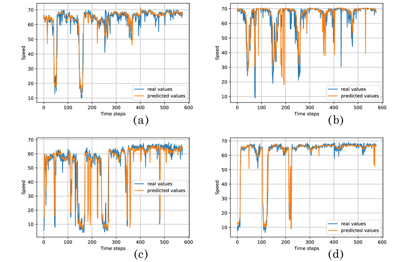
Figure 7. Comparison on 4 randomly selected vertices.

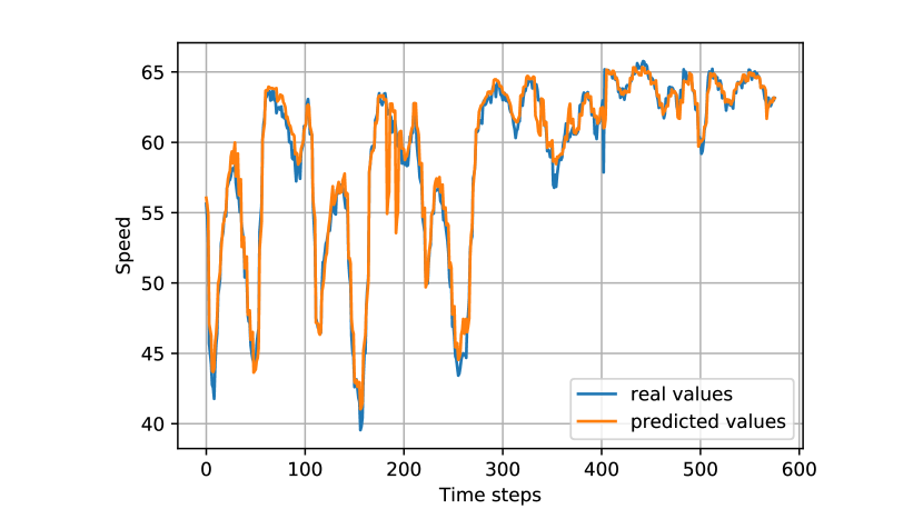
Figure 8. Comparison of average values.

In order to illustrate the performance of our model intuitively, we compared the real values with the predicted values, shown in Figures 7 and 8, respectively. Specifically, we randomly select 4 vertices and arbitrary 576 continuous snapshots (2 days) to compare the real values and predicted values, where the blue lines represent real values while the orange lines denote predicted values. The results of the prediction comparison on specific vertices are shown as Figure 7. Furthermore, in order to compare the overall prediction on all vertices, we compare the real average speed of all vertices in randomly selected 576 continuous snapshots (2 days) with our predicted average speed. The result of prediction comparison of average speed over all vertices is shown as Figure 8.

From Figure 7, we can conclude that our model can fit different patterns of speed change in specific vertices on the micro. From Figure 8, on the macro, our model is able to accurately predict future traffic speed over the whole urban road network.

5. Conclusion

In this paper, we incorporate the perspective of information diffusion to model spatial features and temporal features synchronously in spatial-temporal data. Therefore, we can better preserve its spatial-temporal dependencies. For handling new issues caused by the new perspective, we design three novel key components to improve the performance. On this basis, we propose Iterative Spatial-Temporal Diffusion Graph Convolutional Neural Network (ISTD-GCN). Experiments on two real datasets illustrate that our algorithm outperforms 10 baselines in three tasks.

References

- (1)
- Atluri et al. (2015) Gowtham Atluri, Michael Steinbach, Kelvin O. Lim, Vipin Kumar, and Angus MacDonald. 2015. Connectivity cluster analysis for discovering discriminative subnetworks in schizophrenia. Hum. Brain Map. (2015).
- Ba et al. (2016) Jimmy Lei Ba, Jamie Ryan Kiros, and Geoffrey E. Hinton. 2016. Layer Normalization. arXiv:1607.06450
- Bahdanau et al. (2015) Dzmitry Bahdanau, Kyunghyun Cho, and Yoshua Bengio. 2015. Neural Machine Translation by Jointly Learning to Align and Translate. International Conference on Learning Representation (ICLR). (2015).
- Carney. (2016) Nikita Carney. 2016. All lives matter, but so does race: Black lives matter and the evolving role of social media. Human.Soc. (2016).
- Guo et al. (2019) Shengnan Guo, Youfang Lin, Ning Feng, and Chao Song. 2019. Attention Based Spatial-Temporal Graph Convolutional Networks for Traffic Flow Forecasting. In 33rd AAAI Conference on Artificial Intelligence. (2019).
- H. et al. (1997) Drucker H., Burges C. J., Kaufman L., Smola A. J., and Vapnik V. 1997. Support Vector Regression Machines. Conference on Neural Information Processing Systems (NeurIPS). (1997).
- Hamilton. (1994) James Douglas Hamilton. 1994. Time Series Analysis. Princeton university press Princeton.
- He et al. (2015) Kaiming He, Xiangyu Zhang, Shaoqing Ren, and Jian Sun. 2015. Deep Residual Learning for Image Recognition. Internaltional Conference on Computer Vision and Pattern Recogintion (CVPR) (2015).
- Howard et al. (2017) Andrew G. Howard, Menglong Zhu, Bo Chen, Dmitry Kalenichenko, Weijun Wang, Tobias Weyand, Marco Andreetto, and Hartwig Adam. 2017. MobileNets: Efficient Convolutional Neural Networks for Mobile Vision Applications. Internaltional Conference on Computer Vision and Pattern Recogintion (CVPR). (2017).
- Kalchbrenner et al. (2014) Nal Kalchbrenner, Edward Grefenstette, and Phil Blunsom. 2014. A Convolutional Neural Network for Modelling Sentences. Association for Computational Linguistics (ACL). (2014).
- Kim. (2014) Yoon Kim. 2014. Convolutional Neural Networks for Sentence Classification. Conference on Empirical Methods in Natural Language Processing (EMNLP). (2014).
- Kipf and Welling. (2017) Thomas N. Kipf and Max Welling. 2017. Semi-Supervised Classification with Graph Convolutional Networks. International Conference on Learning Representation (ICLR). (2017).
- Krizhevsky et al. (2012) Krizhevsky, Alex, Sutskever I., and Hinton G. 2012. ImageNet Classification with Deep Convolutional Neural Networks. Conference on Neural Information Processing Systems (NeurIPS). (2012).
- Li et al. (2018a) Qimai Li, Zhichao Han, and Xiao-Ming Wu. 2018a. Deeper Insights into Graph Convolutional Networks for Semi-Supervised Learning. In 32nd AAAI Conference on Artificial Intelligence. (2018).
- Li et al. (2018b) Yaguang Li, Rose Yu, Cyrus Shahabi, and Yan Liu. 2018b. Diffusion Convolutional Recurrent Neural Network: Data-Driven Traffic Forecasting. International Conference on Learning Representations (ICLR). (2018).
- Ma (2017) Xiaolei Ma. 2017. Spatio-temporal Recurrent Convolutional Networks for Traffic Prediction in Transportation Networks. (2017).
- Saha et al. (2010) Suranjana Saha, Shrinivas Moorthi, Hua-Lu Pan, Xingren Wu, Jiande Wang, Sudhir Nadiga, Patrick Tripp, Robert Kistler, John Woollen, David Behringer, and others. 2010. The NCEP climate forecast system reanalysis. Bull. Am. Meteorol. Soc. (2010), 36–44.
- Sandler et al. (2018) Mark Sandler, Andrew Howard, Menglong Zhu, Andrey Zhmoginov, and Liang-Chieh Chen. 2018. MobileNetV2: Inverted Residuals and Linear Bottlenecks. Internaltional Conference on Computer Vision and Pattern Recogintion (CVPR). (2018).
- Shi et al. (2015) Xingjian Shi, Zhourong Chen, Hao Wang, Dit-Yan Yeung, Wai kin Wong, and Wang chun Woo. 2015. Convolutional LSTM Network: A Machine Learning Approach for Precipitation Nowcasting. Conference on Neural Information Processing Systems (NeurIPS). (2015).
- Shuman et al. (2012) David I Shuman, Sunil K Narang, Pascal Frossard, Antonio Ortega, and Pierre Vandergheynst. 2012. The emerging field of signal processing on graphs: Extending high-dimensional data analysis to networks and other irregular domains. arXiv:1211.0053
- Sutskever et al. (2014) Ilya Sutskever, Oriol Vinyals, and Quoc V Le. 2014. Sequence to sequence learning with neural networks. Conference on Neural Information Processing Systems (NeurIPS). (2014).
- Teng (2016) Shang-Hua Teng. 2016. Scalable Algorithms for Data and Network Analysis. Foundations and Trends in Theoretical Computer Science 12 (2016), 1–274.
- Tishby and Zaslavsky. (2015) Naftali Tishby and Noga Zaslavsky. 2015. Deep Learning and the Information Bottleneck Principle. (2015). arXiv:1503.02406
- van den Oord et al. (2016) Aaron van den Oord, Sander Dieleman, Heiga Zen, Karen Simonyan, Oriol Vinyals, Alex Graves, Nal Kalchbrenner, Andrew Senior, , and Koray Kavukcuoglu. 2016. Wavenet: A generative model for raw audio. arXiv:1609.03499
- Wang et al. (2018) Bao Wang, Xiyang Luo, Fangbo Zhang, Baichuan Yuan, Andrea L. Bertozzi, and P. Jeffrey Brantingham. 2018. Graph-Based Deep Modeling and Real Time Forecasting of Sparse Spatio-Temporal Data. arXiv:1804.00684.
- Wu et al. (2019b) Felix Wu, Tianyi Zhang, Amauri Holanda de Souza Jr., Christopher Fifty, Tao Yu, and Kilian Q. Weinberger. 2019b. Simplifying Graph Convolutional Networks. International Conference on Machine Learning (ICML) (2019).
- Wu et al. (2019a) Zonghan Wu, Shirui Pan, Guodong Long, Jing Jiang, and Chengqi Zhang. 2019a. Graph WaveNet for Deep Spatial-Temporal Graph Modeling. International Joint Conference on Artificial Intelligence (IJCAI) (2019).
- Xian et al. (2018) Zhou Xian, Yanyan Shen, Yanmin Zhu, and Linpeng Huang. 2018. Predicting Multi-step Citywide Passenger Demands Using Attention-based Neural Networks. International Conference on Web Search and Data Mining (WSDM). (2018).
- Yu et al. (2018) Bing Yu, Haoteng Yin, and Zhanxing Zhu. 2018. Spatio-Temporal Graph Convolutional Networks: A Deep Learning Framework for Traffic Forecasting. International Joint Conference on Artificial Intelligence (IJCAI). (2018).
- Zhang et al. (2017) Junbo Zhang, Yu Zheng, and Dekang Qi. 2017. Deep Spatio-Temporal Residual Networks for Citywide Crowd Flows Prediction. In 31st AAAI Conference on Artificial Intelligence. (2017).