Unsupervised Deep-Learning Based Deformable Image Registration: A Bayesian Framework

Abstract

Unsupervised deep-learning (DL) models were recently proposed for deformable image registration tasks. In such models, a neural-network is trained to predict the best deformation field by minimizing some dissimilarity function between the moving and the target images. After training on a dataset without reference deformation fields available, such a model can be used to rapidly predict the deformation field between newly seen moving and target images. Currently, the training process effectively provides a point-estimate of the network weights rather than characterizing their entire posterior distribution. This may result in a potential over-fitting which may yield sub-optimal results at inference phase, especially for small-size datasets, frequently present in the medical imaging domain. We introduce a fully Bayesian framework for unsupervised DL-based deformable image registration. Our method provides a principled way to characterize the true posterior distribution, thus, avoiding potential over-fitting. We used stochastic gradient Langevin dynamics (SGLD) to conduct the posterior sampling, which is both theoretically well-founded and computationally efficient. We demonstrated the added-value of our Basyesian unsupervised DL-based registration framework on the MNIST and brain MRI (MGH10) datasets in comparison to the VoxelMorph unsupervised DL-based image registration framework. Our experiments show that our approach provided better estimates of the deformation field by means of improved mean-squared-error ($0.0063$ vs. $0.0065$) and Dice coefficient ($0.73$ vs. $0.71$) for the MNIST and the MGH10 datasets respectively. Further, our approach provides an estimate of the uncertainty in the deformation-field by characterizing the true posterior distribution.

1 Introduction

Deformable image registration is a fundamental task needed in a wide-range of computer vision and image analysis applications. In particular, it plays a key role in the medical imagining domain, where the execution of pre-alignment of 2D/3D voxels is crucial for many medical applications: motion compensation, multi-modal analysis, inter or intra subject alignment for change detection and longitudinal analysis, to name a few [1, 2]. For a comprehensive overview of both classical and deep-learning (DL) based registration methods and their different categories we refer the reader to [3] and [4].

Classical methods formulate the ill-posed deformable registration task as a regularized optimization problem over the deformation fields space and solve it using iterative solvers [5, 6, 7]. Commonly used regularization terms encourage smoothness of the local deformations and ensures desirable properties such as topology-preserving fields [8, 5, 7]. However, these conventional algorithms are computationally demanding, which, in turn, makes the registration of a new pair of images a computationally expensive process.

In light of the success of DL-based methods in numerous computer vision tasks, several studies aimed to propose more efficient and less time-consuming deformable registration approaches based on DL models [9, 10, 11, 12, 13, 14, 15, 16]. These techniques learn a deformation field prediction model either through a supervised learning framework (i.e with the help of provided reference data) [15] or in unsupervised manner [11, 12, 14, 16]. The latter is advantageous as it doesn’t require available reference deformation fields.

However, the current training process effectively provides point-estimates of the neural-network weights rather than characterizing their entire posterior distribution. This may result in a potential over-fitting that yields sub-optimal results at inference phase, especially for small-size datasets commonly present in the medical imaging domain. Further, it lacks the ability to quantify the uncertainty of the deformation field parameter estimates.

Bayesian learning in DL models plays a critical role in improving generalization and assessing the uncertainty of the predictions [17, 18, 19]. In the context of image registration, Yang et al. [15] used an inference-time dropout layer to extend deformation field point-estimates obtained with their QuickSilver supervised registration predictive model to a probabilistic model, enabling the assessment of the uncertainty of the predicted deformation-field. Dalca et al. [14, 13] aimed to characterize the posterior distribution by modeling the latent variable that parameterizes the deformation field with mean and variance parameters in their unsupervised VoxelMorph framework [12]. They introduced a Kullback-Leibler (KL) Divergence term to their loss function to encourage the network prediction toward a normal distribution. A similar method was used by Krebs et al. [16] for cardiac MRI registration. This approach assumes a normally distributed posterior which may result in sub-optimal results in cases of other posterior distributions. While these approaches do provide some mechanism to quantify uncertainty in the deformation field prediction, they do not provide a fully Bayesian characterization of the deformation field posterior distribution.

In a shift from previous approaches, we propose a new, non-parametric, Bayesian unsupervised image registration framework. Our approach does not make any assumptions on the actual posterior distribution. Therefore has the potential to improve upon parametric methods in case of non-normal posterior. We adopt the strategy of stochastic gradient Langevin dynamics (SGLD) [20] to perform the sampling from the posterior distribution of the network weights [17].

SGLD-based training is computationally efficient and suits a wide-range of Bayesian estimation themes encountered in image-processing tasks. For example, Cheng et al. [17], show considerable improvements in unsupervised image denoising by using SGLD to perform posterior sampling in a deep-image-prior denoising model [21]. Further, noise injection to the weights’ gradients has shown additional benefits in training deep and complex models beyond enabling efficient posterior sampling [22]. Some of these are better solutions for non-convex problems, improved generalization ability, and reduced over-fitting, among others. Recently, various studies proposed a version of SGLD that combines both Gaussian noise and adaptive optimization algorithms [23, 22].

Specifically, during the training phase of our framework, we inject Gaussian noise with adaptive variance to the loss gradients and keep all weights obtained after the "burn-in" iteration. We estimate the posterior distribution of the deformation field during inference by averaging deformation field predictions obtained by the model with the saved weights which, in turn, provide robustness to noisy images. In addition, we quantify the uncertainty in the predicted deformation field by calculating the empirical variance of the samples. Our predictive regression model is built upon the VoxelMorph registration system [12]. We use the same network architecture, while incorporating our Bayesian strategy, in both the training and the inference phases. We demonstrated the added-value of our approach on 2D unsupervised registration of both the MNIST [24] and a brain MRI (MGH10) [25] databases.

2 Background: Image Registration

The deformable registration task can be formulated as an optimization problem. Let us denote the pair of fixed and moving images by $I_{f}$ and $I_{M}$, respectively. $\Phi$ is the deformation field, which accounts for mapping the grid of $I_{M}$ to the grid of $I_{f}$. Then, the energy functional that we aim to optimize is:

$$\operatorname*{arg\,min}_{\Phi}{S(I_{f},I_{M}\circ\Phi)+\lambda R(\Phi)}$$ (1)

where $I_{M}\circ\Phi$ denotes the result of warping the moving image with $\Phi$. $S$ is a dissimilarity term, which quantifies the resemblance between the resulted image and the fixed input, and $R$ is a regularization term that encourages the deformation smoothness. The scalar $\lambda$ is a tuning-parameter that accounts for balancing between the two terms, and it controls the smoothness of the resulted deformation. Popular dissimilarity metrics are the mean squared difference/error (MSE), the cross-correlation and the mutual information. The former is used when images have the same dynamic range of intensities while the latter are essential when images exhibit varying gray-levels and different contrasts.
In DL-based registration, the task of the deep model is to predict the deformation:

$$\hat{\Phi}=f_{\theta}(I_{M},I_{F})$$ (2)

where $\theta$ are the parameters of the network and $I_{M},I_{F}$ are the input pairs. It should be emphasized that, in contrast to supervised schemes, unsupervised registration models "learns" the deformation field that maps from $I_{M}$ to $I_{F}$ without providing reference transformation. In the case of non-parametric (free-form) deformation, it predicts $\hat{\Phi}$ by optimizing the following:

$$\hat{\theta}=\operatorname*{arg\,min}_{\theta}{S(I_{F},I_{M}\circ f_{\theta}(I_{M},I_{F}))+\lambda R(f_{\theta}(I_{M},I_{F}))}$$ (3)

3 The Bayesian Approach

From a probabilistic point of view, the network training aims to maximize the posterior estimation of the deformation field parameters:

$$\hat{\theta}=\operatorname*{arg\,max}_{\theta}{P\left(\theta|I_{F},I_{M}\right)\propto P(I_{F},I_{M}|\theta)P(\theta)}$$ (4)

Since direct integration of the posterior distribution is intractable, several approaches proposed to achieve a maximum posterior estimation in a computationally feasible time. The VoxelMorph approach [12] introduced a smoothness regularization term to constrain the deformation field parameters rather than explicitly define the distribution of the deformation field parameters. While this can provide a maximum-a-posterior (MAP) point estimation of the deformation field parameters, it cannot characterize the entire distribution of the deformation field parameters, which may lead to sub-optimal results. In a more recent work, the VoxelMorph approach was extended to provide a characterization of the uncertainty in the deformation field parameters by assuming that the latent variable that parameterizes the deformation field is distributed normally with zero mean and some variance [14, 13]. During the learning process a KL divergence term is introduced to the loss function to encourage the network prediction towards a normal distribution. However, this approach assumes a normally distributed posterior which may result in sub-optimal results in case of other posterior distributions.

Instead, we efficiently sample the actual posterior distribution of the model weights using an adaptive SGLD mechanism. We treat the network weights as random variables and aim to sample the posterior distribution of the model prediction. To this end, we incorporate a noise scheduler that injects a time-dependent Gaussian noise to the gradients of the loss during the optimization process. At every training iteration, we add Gaussian noise with adaptive variance to the loss gradients. Then, the weights are updated in the next iteration according to the "noisy" gradients. This noise schedule can be performed with any stochastic optimization algorithm during the training procedure. In this work we focused on the formulation of the method for the Adam optimizer. We use Gaussian noise with a variance proportional to the learning rate of the Adam optimization algorithm, as it allows the adaption of the noise to the nature of loss curve. Moreover, previous research shows better performance using noise adaptive or time-dependent variance than constant variance [22]. Our adaptive SGLD-based registration (ASGLDReg) strategy is outlined in algorithm 1. The proposed approach can be directly extended to other stochastic optimization algorithms as well.

Input: Tuning parameters $\lambda$ and $\alpha$, and number of epochs $N$

Output: Estimated deformation $\hat{\Phi}$ and registered image $I_{R}$

Data: Dataset of pairs of fixed and moving images $I_{M},I_{F}$

/* The offline training */

1 Function TrainNetwork(${I_{M},I_{F}}$,$\lambda$,$\alpha$,$N$):

2       for $t<N$ do

3             $\tilde{g}^{t}\leftarrow g^{t}+\textbf{N}^{t}$, where $\textbf{N}^{t}\sim\mathcal{N}(0,\frac{s^{t}}{\alpha})$ and $s^{t}$ is the adaptive step size.

4             $\theta^{t+1}\leftarrow\text{{Adam\_Update}}(\theta^{t},\tilde{g}^{t})$

5            

6       end for

7      return $\left\{\theta_{t}\right\}_{t_{b}}^{N}$

8      

9

/* Online Registration */

1 Function FeedForward($I_{M}$,$I_{F}$):

2       Compute a set of deformations $\left\{\Phi_{t}\right\}_{t_{b}}^{N}$ by feed-forwarding $I_{M}$, $\Phi_{t}=f_{\theta^{t}}(I_{M},I_{F})$ for $t\in\left[t_{b},N\right]$

3       Estimate the deformation: $\hat{\Phi}=$$\frac{\sum_{t=t_{b}}^{N}\Phi_{t}}{N-t_{b}}$

4       Register Image: $I_{R}\leftarrow\text{{Spatial\_Transform}}(I_{in},\hat{\Phi}).$

5      

6      return $I_{R},\hat{\Phi}$

7

Algorithm 1 ASGLDReg Algorithm

Offline Training

$L(I_{M},I_{F},f_{\theta}(I_{M},I_{F}))$ denotes the overall registration loss, described in eq.(3), which is composed of both similarity and regularization terms. We denote the loss gradients by:

$$g^{t}\overset{\triangle}{=}\nabla_{\theta}L^{t}(I_{M},I_{F},f_{\theta}(I_{M},I_{F}))$$ (5)

where $t$ is the training iteration (epoch). At each training iteration, Gaussian noise with time-varying variance is added to $g$:

$$\tilde{g}^{t}\leftarrow g^{t}+\textbf{N}^{t}$$ (6)

where $\textbf{N}^{t}\sim\mathcal{N}(0,\frac{s^{t}}{\alpha})$ and $s^{t}$ is the Adam step size. $\alpha$ is a user-selected parameter that controls the noise variance. This is especially important in the first learning stages, which involve a large step size. The network parameters are then updated according to the Adam update rule:

$$\theta^{t+1}\leftarrow\theta^{t}-s^{t}\hat{m}^{t}$$ (7)

where $s^{t}=\frac{\eta}{\sqrt{\hat{v}^{t}+\epsilon}}$, $\hat{m}^{t}$ and $\hat{v}^{t}$ are the bias-corrected versions of the decaying averages of the past gradients and the second moment (squared gradients), respectively:

$$\hat{m}^{t}=\nicefrac{{m^{t}}}{{1-\beta_{1}^{t}}}$$

$$\hat{v}^{t}=\nicefrac{{v^{t}}}{{1-\beta_{2}^{t}}}$$ (8)

where $m^{t}=m^{t-1}+(1-\beta_{1})\tilde{g}^{t}$ and $v^{t}=v^{t-1}+(1-\beta_{2})(\tilde{g}^{t})^{2}$. $\beta_{1}$, $\beta_{2}$ are decay rates and $\eta$ is a fixed constant.

Online Registration

Having the network trained, and its weights during training saved, we exploit only the outputs of the network with weights obtained after the burn-in phase. The burn-in phase is the initial stage of SGLD learning, at which the step size is still relatively large, thus the gradients magnitude dominates the injected noise. After this phase, the step size decays, thus, the injected Gaussian noise will dominate the loss behavior as its curve converges and exhibits only small variations around its steady-state. We sample a set of deformations $\left\{\Phi_{t}\right\}_{t_{b}}^{N}$, obtained by feed-forwarding the pairs ${I_{M},I_{F}}$ to our network after the burn-in phase. $t_{b}$ denotes the cut-off point of the burn-in phase and $N$ is the iterations number. Under some feasible constraints on the step size, the sampled weights converge to the posterior distribution [20]. Thus, outputs of our network after the burn-in phase, trained with the adaptive SGLD approach can be considered as a sampling from the true posterior distribution. Then, when we have a new pair for alignment, we can estimate the averaged posterior deformation:

$$\hat{\Phi}=\frac{\sum_{t=t_{b}}^{N}\Phi_{t}}{N-t_{b}}$$ (9)

Lastly, we register the moving image by resampling its coordinate system with the spatial transform $\hat{\Phi}$. The function Spatial_Transform performs spatial warping as described in [12]. For each pixel $p$, a sub-pixel location $\hat{\Phi}(p)$ in $M$ is calculated. Then, the values are linearly interpolated to obtain an integer.

3.1 Output Statistics

In [17], it is proved that a convolutional network (CNN) with random parameters, which is fed by a stationary input image (such as white noise), acts as a spatial Gaussian process with a stationary kernel. This is valid in the limit as the channels number in each layer goes to infinity. In addition, the authors analyze the network statistical behavior for models with beyond two layers or with more complex systems that incorporate down-sampling, sampling or skip connection. Similar to these conclusions, the deformation obtained by a CNN model with random parameters that operates on stationary pair of images behaves like a Gaussian field. We assume that the network parameters, $\theta$ are Gaussian. In our adaptive learning setting, the latter is accomplished under the assumption of negligible second order moment of Adam, $v^{t}$, i.e. when $\beta_{2}\simeq 1$.

Figure 1: Block diagram of the proposed Bayesian registration system. After having $\left\{\Phi_{t}\right\}_{t_{b}}^{N}$, we calculate the mean and std. of the deformation, $\mu$ and $\sigma$, respectively. Only the mean is used in the registration scheme, but, $\sigma$ provides an estimate of the result uncertainty.

4 The Registration System

Figure 1 illustrates the design of our Bayesian registration framework. Our main building-block is a UNet-based [26] CNN similar to the VoxelMorph model [12]. Given a pair of moving ($I_{M}$) and target ($I_{F}$) images as a 2-channel input, it predicts the deformation field, $\Phi=f_{\theta}(I_{M},I_{F})$. Sampling from the UNet outputs after the burn-in phase is analogous to having a set of stochastic UNets characterized by different weights, each operates on the same pair of moving and fixed images and models the corresponding deformation field. The operation of the system at the inference stage is as follows: it takes a pair of moving ($I_{M}$) and target ($I_{F}$) images as a 2-channel input and predicts the posterior deformation field $\hat{\Phi}$ by computing the average of the deformation field predictions obtained by the stochastic UNets. Lastly, it maps each pixel, $p$, in the moving image to $\hat{\Phi}(p)$ by applying the spatial transform function.

4.1 Network Architecture

Our main UNet-based building block is comprised from encoder and decoder with skip connections. Both encoder and decoder parts consists of CNN layers with kernel size $3\times 3$ followed by Leaky ReLU activation functions. The encoder has $4$ CNN layers, each of $32$ channels, whereas, the decoder consists of $6$ layers with the following number of channels:$\left\{32,32,32,32,32,16\right\}$. Afterwards, a 2-channel convolutional layer is applied on the UNet output to obtain the 2D deformation field. To achieve pyramidal representation of features, from the fine to coarser levels, strided Convolutions are used in the encoder. In the decoder, upsampling, convolutions, and skip connections are applied. Skip connections concatenate features learned in the first four encoder convolutional layers to the first three and fifth decoder layers. In this manner, the decoder output models a 2-channel deformation field of the same size as the fixed and moving images. A detailed description of the VoxelMorph model’s architecture can be found in [12].

4.2 Loss Function

The training process involves the optimization of the energy-functional described in eq. (3). The UNet model is served as an energy optimization solver. We minimize the energy functional w.r.t the network parameters, $\theta$. We use the mean squared error (MSE) for our MNIST experiments and the negative local cross correlation (LCC) for our MRI images experiments to characterize the dissimilarity between the fixed image $I_{F}$ and that obtained after mapping, $I_{M}\circ\hat{\Phi}$. The LCC is commonly used for MRI registration tasks rather than the MSE due to its robustness to intensity changes. Other dissimilarity metrics such as the mutual information [27] can be used as well. We use the $\text{L}_{2}$ norm over the deformation field gradients as a regularization term to encourage the deformation field smoothness. The UNet model then learns the optimal weights by minimizing the loss function composed of the two aforementioned terms.

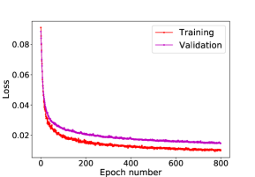
(a)

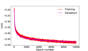
(b)

Figure 2: Loss curves as a function of the training iteration for both MNIST LABEL:sub@fig2:a and MGH10 LABEL:sub@fig2:b datasets. The presented loss consist of both similarity and regularization terms. In the case of MNIST, the loss shows stable behavior after $500$ iterations. However, for the MRI data it reaches a stable phase (for validation) after about $8000$ iterations. Optimal values of the cut-off point, $t_{b}$, should be within these regimes.

5 Experiments

We implement our ASGLDReg method for unsupervised 2D deformable image registration. We use the publicly available implementation of the VoxelMorph model as our building block. Our system was implemented using Keras with a tensorflow backend [28]. We used the MNIST [24] and the MGH10 brain MRI [25] datasetes. The MGH10 dataset consists of brain MRI scans of 10 subjects with provided segmentation into 74 regions. MRI images affine-registered according to the MNI152 template [29], and preprocessed by inhomogeneity-correction. All scans are of size $182\times 218\times 182$ and uniform spacing grid of $1mm$ in each dimension. A detailed description of each experiment follows.

MNIST Registration

We consider deformable registration of pairs of digit $5$ images, which exhibit different geometrical shapes. Data of digit $5$ was randomly split into training, validation and test sets. $199,800$ pairs were produced from $200$ examples that were selected for training, $100$ pairs for validation and $1000$ for the test set. Images were resized to $32\times 32$ and their intensities were normalized to the $\left[0,1\right]$. Our model was trained as outlined in ASGLDReg offline training section with $800$ epochs. We used the Adam optimizer [30] with learning rate of $10^{-3}$ and a batch size of $64$ for training. We added an $L_{2}$ regularization of network weights and biases to our loss function to avoid overfitting. We empirically set the $L_{2}$ regularization weight to $10^{-5}$ and the algorithm input parameters to $\alpha=100$ and $\lambda=0.05$. Figure 2LABEL:sub@fig2:a presents the loss curves as a function of the epoch number, for both the validation and the training sets. The burn-in phase ends after $500$ iterations. Hence, we selected $t_{b}=720$ as the iteration to start the posterior sampling from. A proper selection of $t_{b}$ has an impact on the resulting registration. Lastly, we calculate the mean and variance of the deformations obtained as output of the CNN in iterations ${t_{b},t_{b}+1,...,N}$, and resample the moving image with the averaged deformation to obtain the registered result. The top row of Figure 3 presents an example of a pair of fixed and moving images, the corresponding estimated deformation field, and the resulted warped image from the MNIST database.

MRI Registration

We extracted 10 central 2D slices, images which contain large portions of the brain, from each of the 10 subjects of the MGH10 dataset. We then split the extracted 100 2D images into 64, 16 and 20 examples for training, test and validation, respectively. We generated from these sets $4032$, $240$, $380$ input pairs, respectively. All images were multiplied by their provided brain masks, resized to $128\times 128$ and normalized to the $\left[0,1\right]$ gray-scale domain. Similarly to the MNIST registration above, the network was trained as outlined in ASGLDReg ($\alpha=80$) with $10,000$ iterations. We used the Adam optimizer [30] with the same setting as for the MNIST registration above, except for the learning rate which was set to $0.5^{-3}$. The loss curves for both training and validation sets are highlighted in Figure 2LABEL:sub@fig2:b. The training loss curve shows noisy behavior, however, the validation loss curve is more stable after terminating the burn-in phase (i.e. in iterations larger than $8000$). We selected $t_{b}=9800$ and calculated the mean and variance estimates based on deformations sampled from the range $\left[9800,10000\right]$. An example of the deformation estimates obtained with the system and the corresponding registered result is presented in the bottom row of Figure 3. Additional examples are presented in the supplementary material.

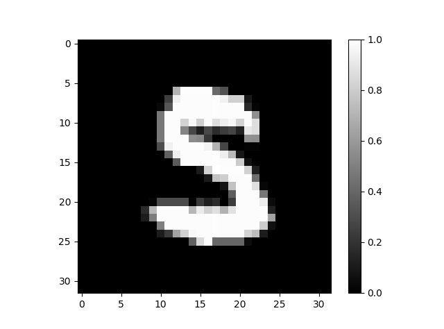
(a) $I_{M}$

(b) $I_{F}$

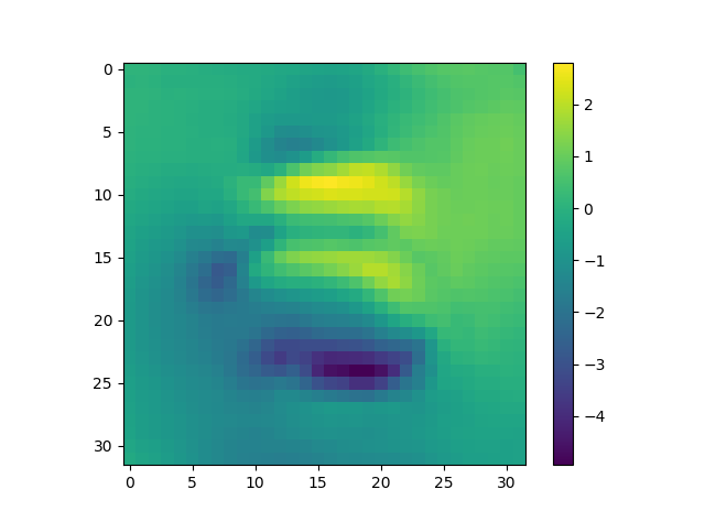
(c) x-component of $\hat{\Phi}$

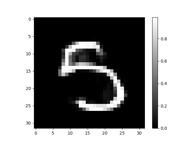
(d) $A_{M}\circ\hat{\Phi}$

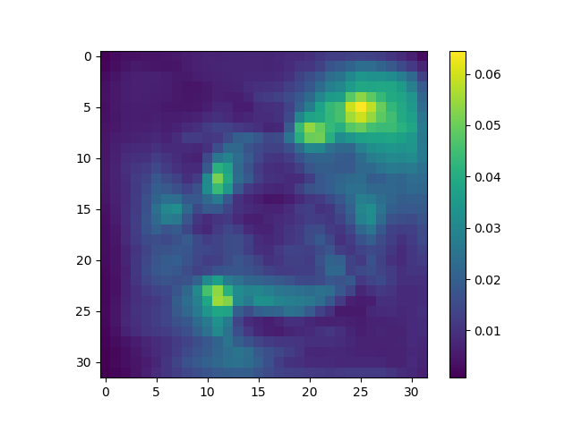
(e) Variance

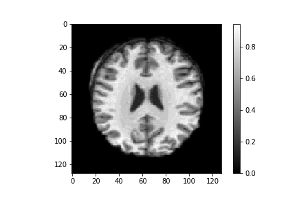
(f) $I_{M}$

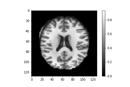
(g) $I_{F}$

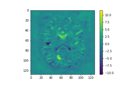
(h) x-component of $\hat{\Phi}$

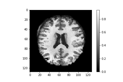
(i) $A_{M}\circ\hat{\Phi}$

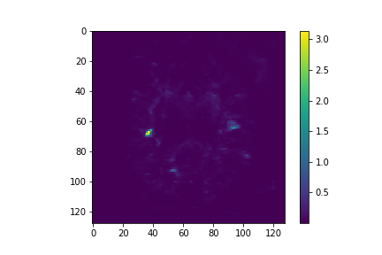
(j) Variance

Figure 3: Registration Results. LABEL:sub@fig3:a, LABEL:sub@fig3:f moving and LABEL:sub@fig3:b, LABEL:sub@fig3:g fixed input images belong to MNIST and MGH10 datasets, respectively. LABEL:sub@fig3:c, LABEL:sub@fig3:h The x-component of the averaged deformation field, calculated after the burn-in. LABEL:sub@fig3:c, LABEL:sub@fig3:h Results of registration obtained by warping the input image with the corresponding deformation field. LABEL:sub@fig3:e, LABEL:sub@fig3:j The variance of the x-component of the predicted deformation field.

Evaluation

We assessed the performance of our Bayesian unsupervised registration system by means of MSE and and Dice score [31] for the MNIST and the MRI registration tasks, respectively. The Dice score measures the registration accuracy by quantifying the volume overlap between a reference segmentation and the propagated (registered) structure. The Dice score varies in the range $\left[0,1\right]$, a Dice score of 1 implies identical structures and complete overlap, while a Dice score of 0 implies no overlap between the sets. We compared three registration methods: our ASGLDReg method with the average over the deformations obtained after the iteration $t_{b}$ (denoted by Averaged), our ASGLDReg method without averaging (i.e considering only the deformation obtained in the last iteration), and the baseline VoxelMorph [12]. We assessed the robustness of our approach against noisy images by corrupting the input images with Gaussian noise with various std. In our MRI registration experiment on MRI data, we considered the largest $4$ anatomical structures present in the images. The mean and std Dice were calculated over the $4$ anatomical structures. A detailed analysis per each structure is provided in the supplementary materials. Table 1 summarizes the quantitative results obtained by the three methods for the different noise levels. Our ASGLDReg method shows a statistically significant improvement (paired Student’s t-test, $p<0.05$ for MNIST and $p<10^{-5}$ for MGH10) upon the VoxelMorph approach for both the MNIST registration (lower MSE) and the MRI registration (higher Dice score) for all noise levels. The added-value of averaging over the posterior samples rather than taking the weights of the last training iteration is more evident in the noisy scenario.

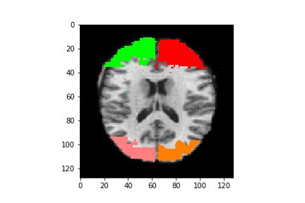
(a) $A_{M}$

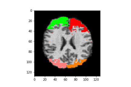
(b) $A_{F}$

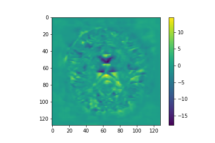
(c) The x-component of $\hat{\Phi}$

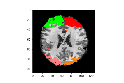
(d) $A_{M}\circ\hat{\Phi}$

Figure 4: Registration Results. LABEL:sub@fig4:a, LABEL:sub@fig4:b moving and fixed input images, annotated with the $4$ anatomical segments, respectively. LABEL:sub@fig4:c The x-component of the corresponding deformation field estimate. LABEL:sub@fig4:d The registered image with the propagated structures after warping with $\hat{\Phi}$.

Table 1: Registration evaluation results for the MNIST and MRI registration experiments. The added noise level is denoted by $\sigma$. For the MRI registration, mean (std) over the different anatomical structures are presented.

	MNIST (MSE)				MGH10 (Dice)
	$\sigma=0$	$\sigma=0.05$	$\sigma=0.1$	$\sigma=0.18$	$\sigma=0$	$\sigma=0.1$	$\sigma=0.18$	$\sigma=0.24$
Averaged	0.0063	0.0077	0.0115	0.0232	0.736 (0.017)	0.732 (0.018)	0.722 (0.018)	0.712 (0.018)
Noisy	$0.0064$	0.0077	$0.0117$	$0.0235$	0.736 (0.017)	$0.731(0.017)$	$0.721(0.018)$	$0.7106(0.017)$
VoxelMorph	$0.0065$	$0.0079$	$0.0122$	$0.0257$	$0.7109(0.027)$	$0.708(0.026)$	$0.699(0.026)$	$0.691(0.026)$

6 Discussion and Conclusions

We proposed a Bayesian unsupervised DL-based registration. We use adaptive noise injection to the training loss gradients to efficiently sample the true posterior distribution of the network weights. Our approach provides empirical estimates of the two principle moments of the deformation field. However, other statistics or higher-order moments can be calculated directly from the posterior samples. Our experiments showed that a Bayesian DL-based registration with posterior sampling through gradient noise injection improves the registration accuracy by means of MSE and Dice score on both the MNSIT and the MGH10 brain MRI databases compared to the point estimates predicted by previously published DL-based registration methods. In our study, we used a 2D version of the VoxelMorph model as the main building-block in which our Bayesian approach method is built upon. However, our proposed Bayesian approach can be extended for 3D registration by replacing the CNN layers from 2D to 3D convolutions. In addition, our model can be extended to ensure diffeomorphic deformation field estimation by using diffeomorphic integration layers [13]. Further, the adaptive posterior sampling proposed here can be generalized to other predictive DL models.

References

- [1] Derek LG Hill, Philipp G Batchelor, Mark Holden, and David J Hawkes. Medical image registration. Physics in medicine & biology, 46(3):R1, 2001.
- [2] Barbara Zitova and Jan Flusser. Image registration methods: a survey. Image and vision computing, 21(11):977–1000, 2003.
- [3] Aristeidis Sotiras, Christos Davatzikos, and Nikos Paragios. Deformable medical image registration: A survey. IEEE transactions on medical imaging, 32(7):1153–1190, 2013.
- [4] Grant Haskins, Uwe Kruger, and Pingkun Yan. Deep learning in medical image registration: A survey. Machine Vision and Applications, 31(1):8, 2020.
- [5] John Ashburner. A fast diffeomorphic image registration algorithm. Neuroimage, 38(1):95–113, 2007.
- [6] Ruzena Bajcsy and Stane Kovačič. Multiresolution elastic matching. Computer vision, graphics, and image processing, 46(1):1–21, 1989.
- [7] Brian B Avants, Charles L Epstein, Murray Grossman, and James C Gee. Symmetric diffeomorphic image registration with cross-correlation: evaluating automated labeling of elderly and neurodegenerative brain. Medical image analysis, 12(1):26–41, 2008.
- [8] M Faisal Beg, Michael I Miller, Alain Trouvé, and Laurent Younes. Computing large deformation metric mappings via geodesic flows of diffeomorphisms. International journal of computer vision, 61(2):139–157, 2005.
- [9] Robin Sandkühler, Simon Andermatt, Grzegorz Bauman, Sylvia Nyilas, Christoph Jud, and Philippe C Cattin. Recurrent registration neural networks for deformable image registration. In Advances in Neural Information Processing Systems, pages 8755–8765, 2019.
- [10] Adrian Dalca, Marianne Rakic, John Guttag, and Mert Sabuncu. Learning conditional deformable templates with convolutional networks. In Advances in neural information processing systems, pages 804–816, 2019.
- [11] Bob D de Vos, Floris F Berendsen, Max A Viergever, Hessam Sokooti, Marius Staring, and Ivana Išgum. A deep learning framework for unsupervised affine and deformable image registration. Medical image analysis, 52:128–143, 2019.
- [12] Guha Balakrishnan, Amy Zhao, Mert R Sabuncu, John Guttag, and Adrian V Dalca. An unsupervised learning model for deformable medical image registration. In Proceedings of the IEEE conference on computer vision and pattern recognition, pages 9252–9260, 2018.
- [13] Adrian V. Dalca, Guha Balakrishnan, John Guttag, and Mert Sabuncu. Unsupervised learning of probabilistic diffeomorphic registration for images and surfaces. Medical Image Analysis, 57:226–236, 2019.
- [14] Adrian V. Dalca, Guha Balakrishnan, John Guttag, and Mert Sabuncu. Unsupervised learning for fast probabilistic diffeomorphic registration. MICCAI: Medical Image Computing and Computer Assisted Intervention, LNCS, 11070:729–738, 2018.
- [15] Xiao Yang, Roland Kwitt, Martin Styner, and Marc Niethammer. Quicksilver: Fast predictive image registration–a deep learning approach. NeuroImage, 158:378–396, 2017.
- [16] Julian Krebs, Hervé Delingette, Boris Mailhé, Nicholas Ayache, and Tommaso Mansi. Learning a probabilistic model for diffeomorphic registration. IEEE transactions on medical imaging, 38(9):2165–2176, 2019.
- [17] Zezhou Cheng, Matheus Gadelha, Subhransu Maji, and Daniel Sheldon. A bayesian perspective on the deep image prior. In Proceedings of the IEEE Conference on Computer Vision and Pattern Recognition, pages 5443–5451, 2019.
- [18] David JC MacKay. A practical bayesian framework for backpropagation networks. Neural computation, 4(3):448–472, 1992.
- [19] Radford M Neal. Bayesian learning for neural networks, volume 118. Springer Science & Business Media, 2012.
- [20] Max Welling and Yee W Teh. Bayesian learning via stochastic gradient langevin dynamics. In Proceedings of the 28th international conference on machine learning (ICML-11), pages 681–688, 2011.
- [21] Dmitry Ulyanov, Andrea Vedaldi, and Victor Lempitsky. Deep image prior. In Proceedings of the IEEE Conference on Computer Vision and Pattern Recognition, pages 9446–9454, 2018.
- [22] Arvind Neelakantan, Luke Vilnis, Quoc V Le, Ilya Sutskever, Lukasz Kaiser, Karol Kurach, and James Martens. Adding gradient noise improves learning for very deep networks. arXiv preprint arXiv:1511.06807, 2015.
- [23] Changyou Chen, David Carlson, Zhe Gan, Chunyuan Li, and Lawrence Carin. Bridging the gap between stochastic gradient mcmc and stochastic optimization. In Artificial Intelligence and Statistics, pages 1051–1060, 2016.
- [24] Yann LeCun. The mnist database of handwritten digits. http://yann. lecun. com/exdb/mnist/, 1998.
- [25] Arno Klein, Jesper Andersson, Babak A Ardekani, John Ashburner, Brian Avants, Ming-Chang Chiang, Gary E Christensen, D Louis Collins, James Gee, Pierre Hellier, et al. Evaluation of 14 nonlinear deformation algorithms applied to human brain mri registration. Neuroimage, 46(3):786–802, 2009.
- [26] Olaf Ronneberger, Philipp Fischer, and Thomas Brox. U-net: Convolutional networks for biomedical image segmentation. In International Conference on Medical image computing and computer-assisted intervention, pages 234–241. Springer, 2015.
- [27] Abhishek Nan, Matthew Tennant, Uriel Rubin, and Nilanjan Ray. Differentiable mutual information and matrix exponential for multi-resolution image registration. In Medical Imaging with Deep Learning, 2020.
- [28] Martín Abadi, Ashish Agarwal, Paul Barham, Eugene Brevdo, Zhifeng Chen, Craig Citro, Greg S Corrado, Andy Davis, Jeffrey Dean, Matthieu Devin, et al. Tensorflow: Large-scale machine learning on heterogeneous distributed systems. arXiv preprint arXiv:1603.04467, 2016.
- [29] Alan C Evans. An mri-based stereotactic atlas from 250 young normal subjects. Soc. neurosci. abstr, 1992, 1992.
- [30] Diederik P Kingma and Jimmy Ba. Adam: A method for stochastic optimization. arXiv preprint arXiv:1412.6980, 2014.
- [31] Lee R Dice. Measures of the amount of ecologic association between species. Ecology, 26(3):297–302, 1945.