Joint Bandwidth Allocation and Path Selection in WANs with Path Cardinality Constraints

Abstract

In this paper, we study a joint bandwidth allocation and path selection problem via solving a multi-objective minimization problem under the path cardinality constraints, namely MOPC. Our problem formulation captures various types of objectives including the proportional fairness, the total completion time, as well as the worst-case link utilization ratio. Such an optimization problem is very challenging since it is highly non-convex. Almost all existing works deal with such a problem using relaxation techniques to transform it to be a convex optimization problem. However, we provide a novel solution framework based on the classic alternating direction method of multipliers (ADMM) approach for solving this problem. Our proposed algorithm is simple and easy to be implemented. Each step of our algorithm consists of either finding the maximal root of a single-cubic equation which is guaranteed to have at least one positive solution or solving a one-dimensional convex subproblem in a fixed interval. Under some mild assumptions, we prove that any limiting point of the generated sequence under our proposed algorithm is a stationary point. Extensive numerical simulations are performed to demonstrate the advantages of our algorithm compared with various baselines.

I Introduction

In wide area networks (WANs), network resource are shared by applications with different high-level performance objectives. For example, high-definition video applications require high throughput for the end users to enjoy video smoothly [1]. Online gaming applications require low latency for better user game experience [2]. AR/VR-based applications such as video conferencing require both high throughput and low latency for data transmission [3]. Note that it is quite challenging to fulfill various performance objectives for these applications. Firstly, there are very limited available bandwidth resources in the network and it is hard to strike a balance across flows with different performance objectives. Secondly, some applications have the advantage of using more than one end-to-end path to deliver the traffic data. This design space of the number of paths also complicates the problem on how to distribute the allocated bandwidth across multiple paths for such flows. Thirdly, there are some underlying limitations on the number of paths an application could use. Such cardinality nature of path selection makes the problem even challenging. In this paper, we will try to address the aforementioned challenges by studying a multi-objective bandwidth allocation and path selection problem with path cardinality constraints.

There are many existing literatures discussing bandwidth allocation and path selection problems in WANs. In [4], an approach called stacked congestion control is proposed to optimize multi-tenant multi-objective performance with a distributed host-based implementation. In [5], a traffic engineering approach in software-defined WANs is proposed to proactively enforce forwarding policies by coordinating the traffic demand of each data center instead of traditional passive control policies relying on given priorities. In [6], a centralized arbiter is used to decide when and at which path each packet should be sent. Even though these approaches demonstrate performance gains compared with baselines therein, they are purely heuristic-based and lack theoretical performance guarantee. A well-known theoretical framework for solving network resource allocation problems is network utility maximization (NUM). In [7], a NUM-based single-objective network problem is solved theoretically with a system-level implementation. However, the approach in [7] can only solve single-objective optimization problems and fails to address the multi-objective requirements in our problem. Furthermore, the above literatures [4, 5, 6, 7] do not address the issue of path cardinality constraints and hence, can not be extended to solve our problem.

The formulation proposed in this paper is built on the foundation of the NUM. Note that without path cardinality constraints, the multi-objective multi-path network resource allocation problem is in fact a convex optimization problem, which can be easily tackled using existing optimization softwares such as cvx [8]. However, if we add the path cardinality constraints to the NUM framework, such a problem becomes an $\ell_{0}$-norm constrained optimization problem, which makes the optimization problem very difficult to solve. The practical meaning of the $\ell_{0}$-norm constraints is to limit the number of paths an application could use. For example, for data backup service, the end users are not sensitive to the arrival sequence of the data packets and the senders can push as much data as possible to the end users with no limitation on the number of paths. For video streaming applications, the user experience heavily depends on the arrival sequence of the data packets and such applications are limited to use just one path to avoid out-of-sequence issue at the end users.

There are some recent works that take path cardinality constraints into consideration in their network resource allocation problems. In [9], a NUM problem with linear objective function and path cardinality constraints is considered. The path cardinality constraints are relaxed using a linear envelope and the solution to the relaxed problem is mapped to a vertex solution using a randomization approach. A theoretical performance gap is analyzed compared with the optimal solution to the relaxed model. However, the approximation and analysis therein cannot be extended to the scenarios with nonlinear objective functions. In [10], a network optimization problem with restrictions in the number of paths and the requirement of delay is considered, which is a mix-integer optimization problem. The authors propose a heuristic solution by first carefully designing the price of each path and develop an algorithm to match the demand of the traffic flows based on ranking the designed prices. However, it is rather hard to have any theoretical analysis on the performance. Note that the above works handle the cardinality constraints by either considering theoretical approximations or heuristic solutions to bypass the associated constraints, which are highly suboptimal and lack performance guarantee.

In this paper, we propose a comprehensive framework for the multi-objective bandwidth allocation and path selection problem with path cardinality constraints. To address the above challenges, we use the ADMM approach to decompose the multi-objective problem into several single-objective subproblems, where we explicitly consider the path cardinality constraints. Then we show that these subproblems are in fact simple to solve even though they are non-convex or quadratic programs. We then theoretically prove the convergence of the proposed algorithm under certain mild conditions and show that it at least achieves suboptimality. Finally, by comparing with several baselines, we show the proposed algorithm has a significant performance gain.

The remainder of the paper is organized as follows. The system model is introduced in Section II. Then two types of bandwidth allocation problems are formulated in Section III. In Section IV, we propose an algorithm to solve the two formulated problems. The convergence analysis is given in Section V. In Section VI, we give the numerical simulations and conclude this paper in Section VII.

II SYSTEM MODEL

We consider a general communication network which is used to deliver data flows from source nodes to destination nodes to facilitate end-to-end data services. Specifically, we consider $K$ flows in the network indexed by $k$ $(k=1,2,\cdots,K)$. There are $L$ uni-directional links indexed by $l$ $(l=1,2,\cdots,L)$ connecting the network nodes with link capacity ${c}_{l}$ $({c}_{l}>0,\forall l)$. We define $\boldsymbol{c}=(c_{1},c_{2},\cdots,c_{L})^{\top}$ as the link capacity vector of the overall network. The centralized network controller is used to govern the overall bandwidth allocation as shown in Figure 1. Specifically, given the utility of each flow (to be illustrated in Section III), the network topology and path cardinality constraints, the network controller will allocate bandwidth and paths to each flow so as to maximize the utilities and achieve load balancing. Furthermore, there is an associated source-destination pair for each $k$-th flow and we assume it will carry data with size $s_{k}$ (in bits). Moreover, for each $k$-th flow, there are $P_{k}$ available paths indexed by $i$ $(i=1,2,\cdots,P_{k},\forall k)$. Let $\boldsymbol{x}_{k}=(x_{k,1},x_{k,2},\cdots,x_{k,P_{k}})^{\top}$ be the bandwidth allocation and path selection vector of the $k$-th flow, where each element $x_{k,i}$ $(x_{k,i}\geq 0,\forall k,i)$ represents the bandwidth allocated at path $i$ for the $k$-th flow (in bits/sec). It can be easily observed that the paths selected by the $k$-th flow are those with positive $x_{k,i}$, i.e., $\{i|x_{k,i}>0\}$. We further define

$$\boldsymbol{x}=\begin{pmatrix}\boldsymbol{x}_{1}\\ \boldsymbol{x}_{2}\\ \vdots\\ \boldsymbol{x}_{K}\end{pmatrix}$$

as the bandwidth allocation and path selection vector of all the flows. We then define the routing matrix, which is a $L\times P_{k}$ matrix representing the relationship between the links and the available paths of the $k$-th flow

$$\boldsymbol{R}_{k}={\left(\begin{array}[]{cccc}R^{k}_{1,1}&R^{k}_{1,2}&\cdots&R^{k}_{1,P_{k}}\\ R^{k}_{2,1}&R^{k}_{2,2}&\cdots&R^{k}_{2,P_{k}}\\ \vdots&\vdots&\ddots&\vdots\\ R^{k}_{L,1}&R^{k}_{L,2}&\cdots&R^{k}_{L,P_{k}}\end{array}\right)},$$

where $R^{k}_{l,i}\in\{0,1\}$. The value $R^{k}_{l,i}=1$ means path $i$ passes link $l$ for the $k$-th flow and vice versa. We define the following $L\times P$ matrix (where we denote $P=\Sigma_{k=1}^{K}P_{k}$) to be the routing matrix of the overall network:

$$\boldsymbol{R}=(\boldsymbol{R}_{1},\boldsymbol{R}_{2},\cdots,\boldsymbol{R}_{K}).$$ (1)

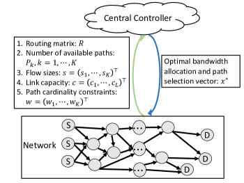
Figure 1: The architecture of our system model with a centralized controller.

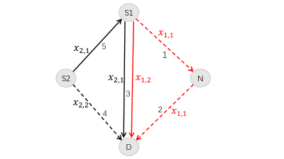
Figure 2: An illustrative example network with five links and two users. The first user (red line), whose source node is $S1$ and destination node is $D$, has rate $x_{1,1}$ and $x_{1,2}$ on its two paths. The second user (black line), whose source node is $S2$ and destination node is $D$, has rate $x_{2,1}$ and $x_{2,2}$ on its two paths. The numbers next to the lines represent the link indices.

Figure 2 gives an example of a small network with five links and two flows (black and red). Each flow has two available paths (solid line and dashed line) and the corresponding routing matrices for the two flows are given by

$$\boldsymbol{R}_{1}={\left(\begin{array}[]{cc}1&0\\ 1&0\\ 0&1\\ 0&0\\ 0&0\end{array}\right)},\boldsymbol{R}_{2}={\left(\begin{array}[]{cc}0&0\\ 0&0\\ 1&0\\ 0&1\\ 1&0\end{array}\right)}.$$

Remark 1.

In general, since each path only passes a small portion of all links over the entire network, $\boldsymbol{R}$ is actually very sparse.

The above network model covers a lot of practical network scenarios. Two examples are illustrated as follows.

Example 1 (Backbone Network): In Backbone network [11], Internet service provider acts as the role of delivering various types of application traffic from multiple data sources to terminal users. The network controller will gather information of traffic flows from the users and content providers on network topology information and traffic requirement information. Then it will optimize and allocate the network bandwidth to different applications under certain constraints on physical link limitations and the number of paths requirements.

Example 2 (Inter Datacenter Network): In Inter-Datacenter Network (IDN) [12], data are required to be migrated from one data center network to another and different applications have different requirements. For instance, video and backup data require high throughput while finance data require low latency. The IDN controller will optimize the data migration process so as to balance the requirements of different applications while achieving load balancing.

III Problem Formulation

In this section, we formulate two types of bandwidth allocation problems. One is the NUM problem [13], in which we use a practical multi-objective utility function to capture both proportional fairness and low total completion time. The other is a multi-objective bandwidth allocation and path selection problem with path cardinality constraints (MOPC). We present the two problems in detail as follows.

III-1 NUM

The NUM [13, 14, 15, 16] is a very popular and practical formulation for bandwidth allocation problems. Let $U_{k}(\|\boldsymbol{x}_{k}\|_{1})$ be the utility of the $k$-th flow, which is a single-variable function and a mapping from the total allocated bandwidth resource to the utility value. We further assume $U_{k}(\cdot)$ is increasing, strictly concave and twice continuously differentiable. Some common choices of $U_{k}(\|\boldsymbol{x}_{k}\|_{1})$ are $\log(\|\boldsymbol{x}_{k}\|_{1})$ and $-\frac{s_{k}}{\|\boldsymbol{x}_{k}\|_{1}}$, which represent the proportional fairness and flow completion time, respectively. In the NUM formulation, the goal is to achieve both proportional fairness and low total completion time among all flows subject to link capacity constraints. For a given positive weight $\beta$, the NUM problem is formulated as

$$\begin{split}\min_{\boldsymbol{x}}\quad&-\sum_{k=1}^{K}U_{k}(\|\boldsymbol{x}_{k}\|_{1})\\ \mbox{s.t.}\quad&\boldsymbol{Rx}\leq\boldsymbol{c}\\ &\boldsymbol{x}\geq 0,\end{split}$$ (2)

where

$$U_{k}(\|\boldsymbol{x}_{k}\|_{1})=\beta\log(\|\boldsymbol{x}_{k}\|_{1})-\frac{s_{k}}{\|\boldsymbol{x}_{k}\|_{1}},\quad\forall k.$$ (3)

III-2 MOPC

Another important goal is to balance network load across links so as to avoid network congestion. Let $\boldsymbol{R}[l]$ be the $l$-th row of the routing matrix $\boldsymbol{R}$ as in (1). Therefore, we consider to include the maximal (or worst-case) link utilization ratio, which is defined as $\max_{l}\frac{\boldsymbol{R}[l]\boldsymbol{x}}{c_{l}}$, in the objective function to reflect the level of load balancing. In addition, path cardinality constraints are added so that the $k$-th flow can be transmitted through at most $w_{k}$ paths, where $w_{k}\leq P_{k}$. Therefore, for given positive weights $\alpha,\beta$, the MOPC problem is formulated as

$$\begin{split}\min_{\boldsymbol{x}}\quad&\sum_{k=1}^{K}-U_{k}(\|\boldsymbol{x}_{k}\|_{1})+\alpha\max_{l}\dfrac{\boldsymbol{R}[l]\boldsymbol{x}}{c_{l}}\\ \mbox{s.t.}\quad&\boldsymbol{Rx}\leq\boldsymbol{c}\\ &\|\boldsymbol{x}_{k}\|_{0}\leq w_{k},\quad\forall\,k\\ &\boldsymbol{x}\geq\boldsymbol{0}.\end{split}$$ (4)

Note that for each $k$, if $w_{k}=P_{k}$, in fact there are no path cardinality constraints on the $k$-th flow. Therefore, our problem formulation (4) is general enough to cover scenarios with various types of constraints on the number of paths.

IV ADMM-based Algorithm Design

In this section, we present our proposed ADMM-based algorithm for solving the NUM and MOPC problems.

IV-A ADMM for NUM

The authors in [15, 16] propose to solve the NUM problem with ADMM. Compared with the approaches in [15, 16], we adopt a different utility function to facilitate our multi-objective optimization problem and also use a different splitting method on the decision variables. Specifically, by introducing the following convex indicator function of link capacity constraints given by

$$\mathcal{I}_{\{\boldsymbol{y}\leq\boldsymbol{c}\}}(\boldsymbol{y})=\begin{cases}0,&if\;\boldsymbol{y}\leq\boldsymbol{c},\\ +\infty,&otherwise,\end{cases}$$ (5)

we can equivalently transform problem in (2) into

$$\begin{split}\min_{\boldsymbol{x},\boldsymbol{y}}\quad&-\sum_{k=1}^{K}U_{k}(\|\boldsymbol{x}_{k}\|_{1})+\mathcal{I}_{\{\boldsymbol{y}\leq\boldsymbol{c}\}}(\boldsymbol{y})\\ \mbox{s.t.}\quad&\boldsymbol{y}=\boldsymbol{Rx}\\ &\boldsymbol{x}\geq\boldsymbol{0}.\end{split}$$ (6)

The augmented Lagrangian function of problem in (6) is then

$$L_{\rho}(\boldsymbol{x},\boldsymbol{y};\boldsymbol{z}) =-\sum_{k=1}^{K}U_{k}(\|\boldsymbol{x}_{k}\|_{1})+\mathcal{I}_{\{\boldsymbol{y}\leq\boldsymbol{c}\}}(\boldsymbol{y})$$

$$+\boldsymbol{z}^{\top}(\boldsymbol{y}-\boldsymbol{Rx})+\dfrac{\rho}{2}\|\boldsymbol{y}-\boldsymbol{Rx}\|_{2}^{2},$$ (7)

where $\boldsymbol{z}$ is a Lagrangian multiplier vector associated with the constraint $\boldsymbol{y}=\boldsymbol{Rx}$ in (6), and $\rho>0$ is a penalty parameter. The ADMM for problem in (6) is derived by alternatively minimizing $L_{\rho}$ in (7) with respect to $\boldsymbol{x}$ and $\boldsymbol{y}$ with the other variables fixed. Specifically, the iterative steps are given by

$$\boldsymbol{x}^{j+1} =\mathop{\arg\min}_{\boldsymbol{x}\geq\boldsymbol{0}}L_{\rho}(\boldsymbol{x},\boldsymbol{y}^{j};\boldsymbol{z}^{j})$$

$$=\mathop{\arg\min}_{\boldsymbol{x}\geq\boldsymbol{0}}-\sum_{k=1}^{K}U_{k}(\|\boldsymbol{x}_{k}\|_{1})+\dfrac{\rho}{2}\|\boldsymbol{y}^{j}-\boldsymbol{Rx}+\frac{\boldsymbol{z}^{j}}{\rho}\|^{2},$$ (8)

$$\boldsymbol{y}^{j+1} =\mathop{\arg\min}_{\boldsymbol{y}}L_{\rho}(\boldsymbol{x}^{j+1},\boldsymbol{y};\boldsymbol{z}^{j})$$

$$=\mathop{\arg\min}_{\boldsymbol{y}\leq\boldsymbol{c}}\dfrac{\rho}{2}\|\boldsymbol{y}-\boldsymbol{Rx}^{j+1}+\frac{\boldsymbol{z}^{j}}{\rho}\|^{2},$$ (9)

where $j$ is the step index, $\boldsymbol{x}^{j+1}=(\boldsymbol{x}_{1}^{j+1};\boldsymbol{x}_{2}^{j+1};\cdots;\boldsymbol{x}_{K}^{j+1})$, and $\boldsymbol{x}_{k}^{j}=(\boldsymbol{x}_{k,1}^{j},\boldsymbol{x}_{k,2}^{j},\cdots,\boldsymbol{x}_{k,P_{k}}^{j})^{\top}$, $\forall k=1,2,\cdots,K$. After the update steps of $\boldsymbol{x}$ and $\boldsymbol{y}$ as above, the update of the multiplier $\boldsymbol{z}$ is given by

$$\boldsymbol{z}^{j+1}=\boldsymbol{z}^{j}+\rho(\boldsymbol{y}^{j+1}-\boldsymbol{Rx}^{j+1}).$$ (10)

We next focus on solving the problems in (8) and (9). For the subproblem in (8), it is hard to get a closed-form solution since $\{\boldsymbol{x}_{k}\}_{k=1,\cdots,K}$ are coupled together due to the quadratic term $\dfrac{\rho}{2}\left\|\boldsymbol{y}^{j}-\boldsymbol{Rx}+\frac{\boldsymbol{z}^{j}}{\rho}\right\|^{2}$. To deal with the coupling issue, we consider linearizing the quadratic term in (8) and adding a proximal term as follows:

$$\boldsymbol{x}^{j+1}$$

$$=\mathop{\arg\min}_{\boldsymbol{x}\geq\boldsymbol{0}}\quad\sum_{k=1}^{K}-U_{k}(\|\boldsymbol{x}_{k}\|_{1})-\rho(\boldsymbol{q}^{j})^{\top}\boldsymbol{x}+\dfrac{\mu}{2}\|\boldsymbol{x}-\boldsymbol{x}^{j}\|^{2}$$

$$=\mathop{\arg\min}_{\boldsymbol{x}\geq\boldsymbol{0}}\quad\sum_{k=1}^{K}-U_{k}(\|\boldsymbol{x}_{k}\|_{1})+\dfrac{\mu}{2}\|\boldsymbol{x}-\boldsymbol{\nu}^{j}\|^{2},$$ (11)

where $\boldsymbol{q}^{j}=\boldsymbol{R}^{\top}(\boldsymbol{y}^{j}-\boldsymbol{Rx}^{j}+\boldsymbol{z}^{j}/\rho)$, $\boldsymbol{\nu}^{j}=\boldsymbol{x}^{j}+(\rho/\mu)\boldsymbol{q}^{j}$, and $\mu>\rho\|\boldsymbol{R}\|_{2}^{2}$. Note that $\boldsymbol{\nu}^{j}=(\boldsymbol{\nu}_{1}^{j};\boldsymbol{\nu}_{2}^{j};\cdots;\boldsymbol{\nu}_{K}^{j})$, and for $\forall k=1,2,\cdots,K$, $\boldsymbol{\nu}_{k}^{j}=(\boldsymbol{\nu}_{k,1}^{j},\boldsymbol{\nu}_{k,2}^{j},\cdots,\boldsymbol{\nu}_{k,P_{k}}^{j})^{\top}$. Therefore based on (11), the problem in the right hand side can be decomposed into several subproblems, where each subproblem only contains one block decision variable $\boldsymbol{x}_{k}$ as follows:

$$\boldsymbol{x}^{j+1}_{k}=\mathop{\arg\min}_{\boldsymbol{x}_{k}\geq\boldsymbol{0}}\quad-U_{k}(\|\boldsymbol{x}_{k}\|_{1})+\dfrac{\mu}{2}\|\boldsymbol{x}_{k}-\boldsymbol{\nu}_{k}^{j}\|^{2},\forall k.$$ (12)

The solution to problem in (12) is then given in the following Lemma 1.

Lemma 1.

The solution of problem in (12) is given by

$$\begin{cases}&x_{k,i}^{j+1}=\max(0,\nu_{k,i}^{j}+\zeta),\quad\forall i,\\ &\mu\zeta=U^{\prime}_{k}\left(\sum_{i=1}^{P_{k}}\max(0,\nu_{k,i}^{j}+\zeta)\right),\end{cases}$$

where $\zeta$ is some positive number. Without loss of generality, suppose the elements of $\boldsymbol{\nu}_{k}^{j}=(\nu_{k,1}^{j},\nu_{k,2}^{j},\cdots,\nu_{k,P_{k}}^{j})^{\top}$ are in descending order. Then if there is some smallest index $i^{\prime}$ $(i^{\prime}\in{2,\cdots,P_{k}})$ such that

$$\mu\zeta\geq U^{\prime}_{k}\left(\sum_{i=1}^{P_{k}}\max(0,\nu_{k,i}^{j}+\zeta)\right),$$

where $\zeta=-\nu_{k,i^{\prime}}^{j}$, we can obtain $\zeta$ through finding the maximal root of a single-variable cubic equation

$$\mu\zeta\left(\sum_{i=1}^{i^{\prime}-1}(\nu^{j}_{k,i}+\zeta)\right)^{2}=\beta\left(\sum_{i=1}^{i^{\prime}-1}(\nu^{j}_{k,i}+\zeta)\right)+s_{k},$$ (13)

otherwise we can obtain $\zeta$ through finding the maximal root of a single-variable cubic equation

$$\mu\zeta\left(\sum_{i=1}^{P_{k}}(\nu^{j}_{k,i}+\zeta)\right)^{2}=\beta\left(\sum_{i=1}^{P_{k}}(\nu^{j}_{k,i}+\zeta)\right)+s_{k}.$$ (14)

Proof.

See Appendix A-A. ∎

For the subproblem in (9), the solution can be easily obtained by performing a projection operation. That is, for $l=1,2,\cdots,L$,

$$y_{l}^{j+1}=\left\{\begin{array}[]{ll}\theta_{l}^{j},&if\quad\theta_{l}^{j}\leq c_{l},\\ c_{l},&otherwise,\end{array}\right.$$ (15)

where $\boldsymbol{\theta}^{j}=\boldsymbol{R}\boldsymbol{x}^{j+1}-\boldsymbol{z}^{j}/\rho$.

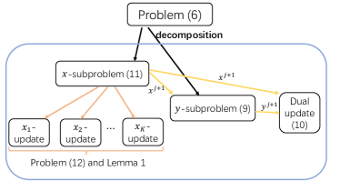
Figure 3: Illustration of the decomposition procedure of our ADMM for NUM.

The overall decomposition procedure using the ADMM approach on the NUM is outlined in Figure 3. Adopting the stopping criteria in the Section 3.3.1 in [17], the complete procedure of our ADMM for NUM is summarized in Algorithm 1.

Algorithm 1 ADMM for the NUM

0:  A randomly initialized point $(\boldsymbol{x}^{0},\boldsymbol{y}^{0},\boldsymbol{z}^{0})$,      set $j=0$, $\rho>0$, and $\mu>\rho\|\boldsymbol{R}\|^{2}$.

0:  An optimal bandwidth allocation and path selection vector $\boldsymbol{x}^{*}$.

1:  while The stopping criteria (see Section 3.3.1 in [17]) are not satisfied do

2:     (Solve the $\boldsymbol{x}$-minimization problem in (12) according to Lemma 1)

3:     for $k=1\to K$ do

4:        Sort the elements of $\boldsymbol{\nu}^{j}_{k}$ in descending order.

5:        Try every positive $\zeta=-\nu^{j}_{k,i}(i=2,\cdots,P_{k})$ to determine the corresponding interval in which $\zeta$ satisfies $\mu\zeta=U^{\prime}_{k}\left(\sum_{i=1}^{P_{k}}\max(0,\nu^{j}_{k,i}+\zeta)\right)$.

6:        Solve the single-variable cubic equation in (13) or (14).

7:        Let $x_{k,i}^{j+1}=\max(0,\nu^{j}_{k,i}+\zeta),\quad\forall i$.

8:     end for

9:     (Solve the $\boldsymbol{y}$-minimization problem (9) with (15))

10:     Compute $\boldsymbol{\theta}^{j}=\boldsymbol{R}\boldsymbol{x}^{j+1}-\boldsymbol{z}^{j}/\rho$.

11:     For each $l=1,\cdots,L$, perform

$$y_{l}^{j+1}=\left\{\begin{array}[]{ll}\theta^{j}_{l},&if\quad\theta^{j}_{l}\leq c_{l},\\ c_{l},&otherwise.\end{array}\right.$$

12:     Update the multiplier $\boldsymbol{z}$ according to (10).

13:     Set $j=j+1$.

14:  end while

IV-B ADMM for MOPC

In this subsection, we solve the MPOC using the ADMM approach. We first transform (4) into the following equivalent form:

$$\begin{split}\min_{\boldsymbol{x}\in\mathcal{X},\boldsymbol{y}\in\mathcal{Y}}\quad&\sum_{k=1}^{K}-U_{k}(\|\boldsymbol{x}_{k}\|_{1})+\alpha\max_{l}\dfrac{y_{l}}{c_{l}}\\ \mbox{s.t.}\quad&\boldsymbol{y}=\boldsymbol{Rx},\end{split}$$ (16)

where $\mathcal{X}=\{\boldsymbol{x}|\|\boldsymbol{x}_{k}\|_{0}\leq w_{k},\,\forall k;\boldsymbol{x}\geq\boldsymbol{0}\}$, and $\mathcal{Y}=\{\boldsymbol{y}|\boldsymbol{0}\leq\boldsymbol{y}\leq\boldsymbol{c}\}$. The augmented Lagrangian function of problem in (16) is

$$L_{\rho}(\boldsymbol{x},\boldsymbol{y};\boldsymbol{z}) =\sum_{k=1}^{K}-U_{k}(\|\boldsymbol{x}_{k}\|_{1})+\alpha\max_{l}\dfrac{y_{l}}{c_{l}}$$

$$+\boldsymbol{z}^{\top}(\boldsymbol{y}-\boldsymbol{Rx})+\dfrac{\rho}{2}\|\boldsymbol{y}-\boldsymbol{Rx}\|_{2}^{2},$$ (17)

where $\boldsymbol{z}$ is a Lagrangian multiplier vector associated with the constraint $\boldsymbol{y}=\boldsymbol{Rx}$ in (16) and $\rho>0$ is a penalty parameter.

Similar to the ADMM for the NUM, the ADMM for the MOPC problem in (16) performs minimization of $L_{\rho}$ in (17) with respect to $\boldsymbol{x}$ and $\boldsymbol{y}$ alternatively followed by the update of $\boldsymbol{z}$. That is, at iteration $j$, the following updates of variables are performed:

$$\boldsymbol{x}^{j+1} =\mathop{\arg\min}_{\boldsymbol{x}\in\mathcal{X}}L_{\rho}(\boldsymbol{x},\boldsymbol{y}^{j};\boldsymbol{z}^{j})$$

$${=\mathop{\arg\min}_{\boldsymbol{x}\in\mathcal{X}}\sum_{k=1}^{K}-U_{k}(\|\boldsymbol{x}_{k}\|_{1})+\dfrac{\rho}{2}\|\boldsymbol{y}^{j}-\boldsymbol{Rx}+\frac{\boldsymbol{z}^{j}}{\rho}\|^{2},}$$ (18)

$$\boldsymbol{y}^{j+1} =\mathop{\arg\min}_{\boldsymbol{y}\in\mathcal{Y}}L_{\rho}(\boldsymbol{x}^{j+1},\boldsymbol{y};\boldsymbol{z}^{j})$$

$$=\mathop{\arg\min}_{\boldsymbol{y}\in\mathcal{Y}}\alpha\max_{l}\dfrac{y_{l}}{c_{l}}+\dfrac{\rho}{2}\|\boldsymbol{y}-\boldsymbol{Rx}^{j+1}+\frac{\boldsymbol{z}^{j}}{\rho}\|^{2},$$ (19)

$$\boldsymbol{z}^{j+1} =\boldsymbol{z}^{j}+\rho(\boldsymbol{y}^{j+1}-\boldsymbol{Rx}^{j+1}).$$ (20)

We next focus on solving the subproblem in (18). Similar to the technique in solving (8), we also consider linearizing the quadratic term in (18) and adding a proximal term:

$$\boldsymbol{x}^{j+1}$$

$$=\mathop{\arg\min}_{\boldsymbol{x}\in\mathcal{X}}\quad\sum_{k=1}^{K}-U_{k}(\|\boldsymbol{x}_{k}\|_{1})-\rho(\boldsymbol{q}^{j})^{\top}\boldsymbol{x}+\dfrac{\mu}{2}\|\boldsymbol{x}-\boldsymbol{x}^{j}\|^{2}$$

$$=\mathop{\arg\min}_{\boldsymbol{x}\in\mathcal{X}}\quad\sum_{k=1}^{K}-U_{k}(\|\boldsymbol{x}_{k}\|_{1})+\dfrac{\mu}{2}\|\boldsymbol{x}-\boldsymbol{\nu}^{j}\|^{2},$$ (21)

where $\boldsymbol{q}^{j}=\boldsymbol{R}^{\top}(\boldsymbol{y}^{j}-\boldsymbol{Rx}^{j}+\boldsymbol{z}^{j}/\rho),\boldsymbol{\nu}^{j}=\boldsymbol{x}^{j}+(\rho/\mu)\boldsymbol{q}^{j}$, and $\mu>\rho\|\boldsymbol{R}\|^{2}$. We decompose (21) into several subproblems, where each subproblem is associated with only one block $\boldsymbol{x}_{k}$,

$$\boldsymbol{x}^{j+1}_{k}=\mathop{\arg\min}_{\|\boldsymbol{x}_{k}\|_{0}\leq w_{k},\boldsymbol{x}_{k}\geq\boldsymbol{0}}-U_{k}(\|\boldsymbol{x}_{k}\|_{1})+\dfrac{\mu}{2}\|\boldsymbol{x}_{k}-\boldsymbol{\nu}_{k}^{j}\|^{2},\forall k.$$ (22)

Leveraging the strict concaveness and monotonicity of the utility function $U_{k}(\cdot)$ in $(0,+\infty)$, we obtain the solution to (22) in the following two lemmas as well as Lemma 1.

Lemma 2.

If $w_{k}=1$, for block $\boldsymbol{x}_{k}$, we denote $i\,(i\in\{1,2,\cdots,P_{k}\})$ as the index where $\nu_{k,i}^{j}$ attains the maximal value, then only the $i$-th element of $\boldsymbol{x}_{k}^{j+1}$, i.e., $x_{k,i}^{j+1}$ is non-zero and its value is the maximal root of a single-variable cubic equation

$$\mu\left(x_{k,i}^{j+1}\right)^{3}-\mu\nu_{k,i}^{j}\left(x_{k,i}^{j+1}\right)^{2}-\beta\left(x_{k,i}^{j+1}\right)-s_{k}=0,\,\forall k,$$ (23)

which always has at least one positive root.

Proof.

See Appendix A-B. ∎

Lemma 3.

If $1<w_{k}<P_{k}$, without loss of generality, suppose the elements of $\boldsymbol{\nu}_{k}^{j}$ are in descending order. Then one of its solutions (there may exist “many” solutions because $\boldsymbol{\nu}_{k}^{j}$ may have equal elements) satisfies

$$x_{k,i}^{j+1}=\max(0,\nu^{j}_{k,i}+\zeta),\quad i=1,\cdots,w_{k},$$ (24a)

$$\mu\zeta=U^{\prime}_{k}\left(\sum_{i=1}^{w_{k}}\max(0,\nu^{j}_{k,i}+\zeta)\right),$$ (24b)

$$x_{k,i}^{j+1}=0,\quad i>w_{k},$$ (24c)

Where $\zeta$ is some positive number. If there is some smallest index $i^{\prime}$ $(i^{\prime}\in{2,\cdots,w_{k}})$ such that

$$\mu\zeta\geq U^{\prime}_{k}\left(\sum_{i=1}^{w_{k}}\max(0,\nu_{k,i}^{j}+\zeta)\right),$$

where $\zeta=-\nu_{k,i^{\prime}}^{j}$, we can obtain $\zeta$ through finding the maximal root of a single-variable cubic equation

$$\mu\zeta\left(\sum_{i=1}^{i^{\prime}-1}(\nu^{j}_{k,i}+\zeta)\right)^{2}=\beta\left(\sum_{i=1}^{i^{\prime}-1}(\nu^{j}_{k,i}+\zeta)\right)+s_{k},$$ (25)

otherwise we can obtain $\zeta$ through finding the maximal root of a single-variable cubic equation

$$\mu\zeta\left(\sum_{i=1}^{w_{k}}(\nu^{j}_{k,i}+\zeta)\right)^{2}=\beta\left(\sum_{i=1}^{w_{k}}(\nu^{j}_{k,i}+\zeta)\right)+s_{k}.$$ (26)

Proof.

See Appendix A-C. ∎

Remark 2.

It is worth noting that the $\boldsymbol{x}$-subproblem in (21) can be solved in a parallel manner because it can be decomposed into several independent subproblems in (22), each of which involves only one block variable $\boldsymbol{x}_{k}$.

Note that it is quite hard to obtain a closed-form solution to the subproblem in (19) since it is a non-smooth problem with linear constraints. By introducing a new variable $t=\max_{l}\dfrac{y_{l}}{c_{l}}$, we transform it into an equivalent quadratic program

$$\begin{split}\min_{t,\boldsymbol{y}}\quad&\phi(t,\boldsymbol{y})=\alpha t+\dfrac{\rho}{2}\|\boldsymbol{y}-\boldsymbol{Rx}^{j+1}+\boldsymbol{z}^{j}/\rho\|^{2}\\ \mbox{s.t.}\quad&\boldsymbol{y}\leq t\boldsymbol{c}\\ &\boldsymbol{y}\geq\boldsymbol{0}\\ &\boldsymbol{y}\leq\boldsymbol{c}.\end{split}$$ (27)

The solution to problem (27) (equivalently problem (19)) is given as follows:

Lemma 4.

Consider problem (27). Let $t^{*}$ be the optimal solution to

$$\min_{t}\Phi(t)=\phi(t,\boldsymbol{y}(t))\quad s.t.\quad 0\leq t\leq 1,$$ (28)

where $\boldsymbol{y}(t)=(y_{1}(t),\cdots,y_{L}(t))^{\top}$ and $y_{l}(t),l=1,\cdots,L$ are defined by

$$y_{l}(t)=\left\{\begin{array}[]{ll}\theta^{j}_{l},&if\quad 0\leq\theta^{j}_{l}\leq\min(c_{l},tc_{l}),\\ \min(c_{l},tc_{l}),&if\quad\theta^{j}_{l}>\min(c_{l},tc_{l}),\\ 0,&otherwise,\end{array}\right.$$ (29)

where $\boldsymbol{\theta}^{j}=\boldsymbol{Rx}^{j+1}-{\boldsymbol{z}^{j}}/\rho$. Then $(t^{*},\boldsymbol{y}(t^{*}))$ is the optimal solution to problem (27) and $\boldsymbol{y}(t^{*})$ is the optimal solution to problem (19). Solving problem (28) is to minimize a single-variable convex function on a closed interval, which can be solved by golden section search and parabolic interpolation (e.g., the function “fminbnd” [18, 19] in MATLAB).

Proof.

See Appendix A-D. ∎

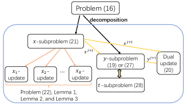
Figure 4: Illustration of the decomposition procedure of our ADMM for MOPC.

Figure 4 gives the overall decomposition procedure using the ADMM approach on the MOPC. The complete procedure of ADMM for MOPC is summarized in Algorithm 2.

Algorithm 2 ADMM for the MOPC

0:  A randomly initialized point $(\boldsymbol{x}^{0},\boldsymbol{y}^{0},\boldsymbol{z}^{0})$, $w_{k}\,(k=1,2,\cdots,K)$, $j=0$, $\rho>0$, and $\mu>\rho\|\boldsymbol{R}\|^{2}.$

0:  The optimal bandwidth allocation and path selection vector $\boldsymbol{x}^{*}$ and corresponding $\boldsymbol{y}^{*}$.

1:  while The stopping criteria (stated in Section VI-B) are not satisfied do

2:     (Solve the $\boldsymbol{x}$-minimization problem in (22))

3:     for $k=1\to K$ do

4:        if $w_{k}=1$ then

5:           Solve the single-variable cubic equation in (23) to get $\boldsymbol{x}^{j+1}_{k}$.

6:        else if $1<w_{k}<P_{k}$ then

7:           Sort the elements of $\boldsymbol{\nu}^{j}_{k}$ in descending order.

8:           Try every positive $\zeta=-\nu^{j}_{k,i}(i=2,\cdots,w_{k})$ to determine the corresponding interval in which $\zeta$ satisfies $\mu\zeta=U^{\prime}_{k}\left(\sum_{i=1}^{w_{k}}\max(0,\nu^{j}_{k,i}+\zeta)\right)$.

9:           Solve the single-variable cubic equation in (25) or (26).

10:           Get $x_{k,i}^{j+1}$ according to (24a) and (24c).

11:        else

12:           Sort the elements of $\boldsymbol{\nu}^{j}_{k}$ in descending order.

13:           Try every positive $\zeta=-\nu^{j}_{k,i}(i=2,\cdots,P_{k})$ to determine the corresponding interval in which $\zeta$ satisfies $\mu\zeta=U^{\prime}_{k}\left(\sum_{i=1}^{P_{k}}\max(0,\nu^{j}_{k,i}+\zeta)\right)$.

14:           Solve the single-variable cubic equation in (13) or (14).

15:           Let $x_{k,i}^{j+1}=\max(0,\nu^{j}_{k,i}+\zeta),\quad\forall i$.

16:        end if

17:     end for

18:     (Solve the $\boldsymbol{y}$-minimization problem (19) according to Lemma 4)

19:     Solve the single-variable optimization problem in (28) using “fminbnd” in MATLAB to get the optimal $t$.

20:     Get $\boldsymbol{y}^{j+1}$ with (29).

21:     Update the multiplier $\boldsymbol{z}$ according to (20).

22:     Set $j=j+1$.

23:  end while

V Convergence Analysis

In this section, we analyze the convergence property of the proposed algorithm in Algorithm 2. As for Algorithm 1, since the NUM in (2) is a convex problem, the convergence of Algorithm 1 has already been well studied in [17] and [20]. For simplicity of notation, we rewrite problem (16) as

$$\begin{split}\min_{\boldsymbol{x},\boldsymbol{y}}\quad&f(\boldsymbol{x})+g(\boldsymbol{y})+\mathcal{I}_{\mathcal{Y}}(\boldsymbol{y})+\mathcal{I}_{\mathcal{X}}(\boldsymbol{x})\\ \mbox{s.t.}\quad&\boldsymbol{y}=\boldsymbol{Rx},\end{split}$$ (30)

where

$$f(\boldsymbol{x})=\sum_{k=1}^{K}-U_{k}(\sum_{i=1}^{P_{k}}x_{k,i}),$$

$$g(\boldsymbol{y})=\alpha\max_{l}\dfrac{y_{l}}{c_{l}},$$

and $\mathcal{I}_{\mathcal{Y}}(\boldsymbol{y})$ as well as $\mathcal{I}_{\mathcal{X}}(\boldsymbol{x})$ are indicator functions defined in (5). The augmented Lagrangian function can be rewritten as

$$L_{\rho}(\boldsymbol{x},\boldsymbol{y};\boldsymbol{z})=f(\boldsymbol{x})+g(\boldsymbol{y})+\mathcal{I}_{\mathcal{X}}(\boldsymbol{x})+\mathcal{I}_{\mathcal{Y}}(\boldsymbol{y})$$

$$+\boldsymbol{z}^{\top}(\boldsymbol{y}-\boldsymbol{R}\boldsymbol{x})+\frac{\rho}{2}\|\boldsymbol{y}-\boldsymbol{R}\boldsymbol{x}\|^{2}.$$ (31)

Next, we show the boundedness of the augmented Lagrangian function, which plays an important role in our convergence analysis.

Proposition 1.

Assume that $\{\boldsymbol{z}^{j}\}$ is bounded, then the sequence of the augmented Lagrangian $\{L_{\rho}(\boldsymbol{x}^{j},\boldsymbol{y}^{j};\boldsymbol{z}^{j})\}_{j=1}^{+\infty}$ is bounded below.

Proof.

See Appendix A-E. ∎

Even through the function $\mathcal{I}_{\mathcal{X}}(\boldsymbol{x})$ is non-smooth and non-convex, we know from [21] and [22] that there exists limiting subdifferential or simply the subdifferential for it, written as $\partial\mathcal{I}_{\mathcal{X}}(\boldsymbol{x})$.

In the rest of this paper, for simplicity, the following notations are used for the successive errors of the iterative sequence:

$$E_{\boldsymbol{x}}^{j+1}\coloneqq\boldsymbol{x}^{j+1}-\boldsymbol{x}^{j},E_{\boldsymbol{y}}^{j+1}\coloneqq\boldsymbol{y}^{j+1}-\boldsymbol{y}^{j},E_{\boldsymbol{z}}^{j+1}\coloneqq\boldsymbol{z}^{j+1}-\boldsymbol{z}^{j}.$$

Before proceeding with our proof, we first show the KKT conditions of problem in (30) and the optimality conditions of the subproblems of ADMM. The KKT conditions of problem (30) are there exists $\hat{\boldsymbol{z}}^{*}\in\mathcal{R}^{L}$, such that

$$\boldsymbol{0}\in\nabla f(\boldsymbol{x}^{*})+\partial\mathcal{I}_{\mathcal{X}}(\boldsymbol{x}^{*})-\boldsymbol{R}^{\top}\hat{\boldsymbol{z}}^{*},$$ (32a)

$$\boldsymbol{0}\in\partial g(\boldsymbol{y}^{*})+\partial\mathcal{I}_{\mathcal{Y}}(\boldsymbol{y}^{*})+\hat{\boldsymbol{z}}^{*},$$ (32b)

$$\boldsymbol{y}^{*}=\boldsymbol{R}\boldsymbol{x}^{*}.$$ (32c)

The first-order optimality condition of $\boldsymbol{x}$-subproblem in (21) is

$$\exists\,\tilde{\boldsymbol{x}}^{j+1}\in\partial\mathcal{I}_{\mathcal{X}}(\boldsymbol{x}^{j+1}),\text{such that}$$

$$\nabla f(\boldsymbol{x}^{j+1})+\tilde{\boldsymbol{x}}^{j+1}-\rho\boldsymbol{q}^{j}+\mu(\boldsymbol{x}^{j+1}-\boldsymbol{x}^{j})=\boldsymbol{0},$$ (33)

The first-order optimality condition of $\boldsymbol{y}$-subproblem in (19) is

$$\exists\,\tilde{\boldsymbol{g}}^{j+1}\in\partial g(\boldsymbol{y}^{j+1}),\text{and}\;\exists\,\tilde{\boldsymbol{y}}^{j+1}\in\partial\mathcal{I}_{\mathcal{Y}}(\boldsymbol{y}^{j+1}),\text{such that}$$

$$\tilde{\boldsymbol{g}}^{j+1}+\tilde{\boldsymbol{y}}^{j+1}+\rho(\boldsymbol{y}^{j+1}-\boldsymbol{Rx}^{j+1}+\boldsymbol{z}^{j}/\rho)=\boldsymbol{0},$$ (34)

which is equivalent to

$$\tilde{\boldsymbol{g}}^{j+1}+\tilde{\boldsymbol{y}}^{j+1}+\boldsymbol{z}^{j+1}=\boldsymbol{0}.$$ (35)

Next, we estimate the differences of the augmented Lagrangian function values between two successive iterations of Algorithm 2 to show the sufficient decrease.

Lemma 5.

For all $j\geq 0$, we have

$$L_{\rho}(\boldsymbol{x}^{j},\boldsymbol{y}^{j};\boldsymbol{z}^{j})-L_{\rho}(\boldsymbol{x}^{j+1},\boldsymbol{y}^{j+1};\boldsymbol{z}^{j+1})+\frac{1}{\rho}\|E_{\boldsymbol{z}}^{j+1}\|^{2}$$

$$\geq\frac{\mu-\rho\|\boldsymbol{R}\|_{2}^{2}}{2}\|E_{\boldsymbol{x}}^{j+1}\|^{2}+\frac{\rho}{2}\|E_{\boldsymbol{y}}^{j+1}\|^{2}.$$ (36)

Proof.

See Appendix A-F. ∎

At this point, we readily have the following theorem regarding the optimality of the output of Algorithm 2.

Theorem 1.

Let $\{\boldsymbol{x}^{j},\boldsymbol{y}^{j},\boldsymbol{z}^{j}\}_{j=1}^{+\infty}$ be a sequence generated by Algorithm 2 and assume that

$$\sum_{j=1}^{\infty}\|E_{\boldsymbol{z}}^{j+1}\|^{2}<\infty\text{ and }\{\boldsymbol{z}^{j}\}\text{ is bounded}.$$

Then, the sequence $\{\boldsymbol{x}^{j},\boldsymbol{y}^{j}\}_{j=1}^{+\infty}$ is bounded and any limiting point $\{\overline{\boldsymbol{x}},\overline{\boldsymbol{y}}\}$ of $\{\boldsymbol{x}^{j},\boldsymbol{y}^{j}\}_{j=1}^{+\infty}$ is a stationary point of problem in (30).

Proof.

See Appendix A-G. ∎

Remark 3.

Note that our problem in (16) or (30) is non-convex and non-smooth, which is in general almost impossible to get a global optimal solution. The above theorem means that any accumulation point that our algorithm generates is a critical point, which is suboptimal to our problem in (16) or (30).

VI Numerical Simulations

In this section, we perform numerical simulations to illustrate the performance gain of our algorithm by comparing several baselines. We first consider a baseline by adopting the convex relaxation approach in [9] to solve our MOPC in (4). Specifically, we relax the $\ell_{0}$-norm constraints in (4) to linear constraints using the relaxation technique in [9]. First the nonlinear term $\max_{l}\frac{\boldsymbol{R}[l]\boldsymbol{x}}{c_{l}}$ in the objective function is transformed to a linear objective function and some constraints by introducing an auxiliary variable $t$. After such linear relaxation and linear representation, (4) is transformed as

$$\begin{split}\min_{\boldsymbol{x},t}\quad&-\sum_{k=1}^{K}U_{k}(\|\boldsymbol{x}_{k}\|_{1})+\alpha t\\ \mbox{s.t.}\quad&\boldsymbol{Rx}\leq t\boldsymbol{c}\\ &\sum_{i=1}^{P_{k}}\frac{x_{k,i}}{\hat{c}_{k,i}}\leq w_{k},\quad\forall\,k\\ &\boldsymbol{x}\geq\boldsymbol{0}\\ &0\leq t\leq 1,\end{split}$$ (37)

where $\hat{c}_{k,i}=\min_{l}\{c_{l}|R_{l,i}^{k}=1\}$ can be interpreted as the capacity of the bottleneck link along path $i$ of $k$-th flow [9]. We solve the above problem via the conditional gradient method (also called the Frank-Wolfe method) [23], which serves as one of our baselines.

VI-A Dataset Descriptions

We perform our simulations based on the data obtained from practical real WAN. Specifically, the flow size vector $\boldsymbol{s}$, the link capacity vector $\boldsymbol{c}$, the routing matrix $\boldsymbol{R}$ and vector $\boldsymbol{w}$ (the number of paths each flow is allowed to use) are configured as follows:

• $\boldsymbol{R}$: $\boldsymbol{R}\in\mathbb{R}^{L\times P}$ with $L=460$, and $P=19751$ from a practical network.

• $P_{k},\,(k=1,\cdots,K)$: Ranging from 4 to 100. The cumulative distribution function of $\{P_{k}\}_{k=1}^{K}$ is plotted in Figure 5(a).

• $\boldsymbol{c}$: Ranging from $1.024\times 10^{9}$ bits/sec to $2.048\times 10^{11}$ bits/sec. The cumulative distribution function of link capacity is plotted in Figure 5(b).

• $\boldsymbol{s}$: We generate a total number of 561 aggregate flows and the size of each is constructed as follows: First we generate several flows (the number of flows is randomly chosen from $[10^{3},10^{4}]$) according to one kind of flow size distribution randomly chosen from the five typical flow size distributions [24] available, which are plotted in Figure 6(a). Next those generated flows are aggregated to be one flow and the size of each aggregate flow is the total size of flows in that aggregate one. Our generated $\boldsymbol{s}$ is plotted in Figure 6(b).

• $\boldsymbol{w}$: We generate $w_{k}$ randomly from $\{1,2,3\}$.

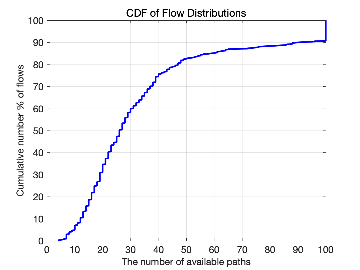
(a) The cumulative distribution function of the number of total available paths $P_{k},\;(k=1,\cdots,K)$.

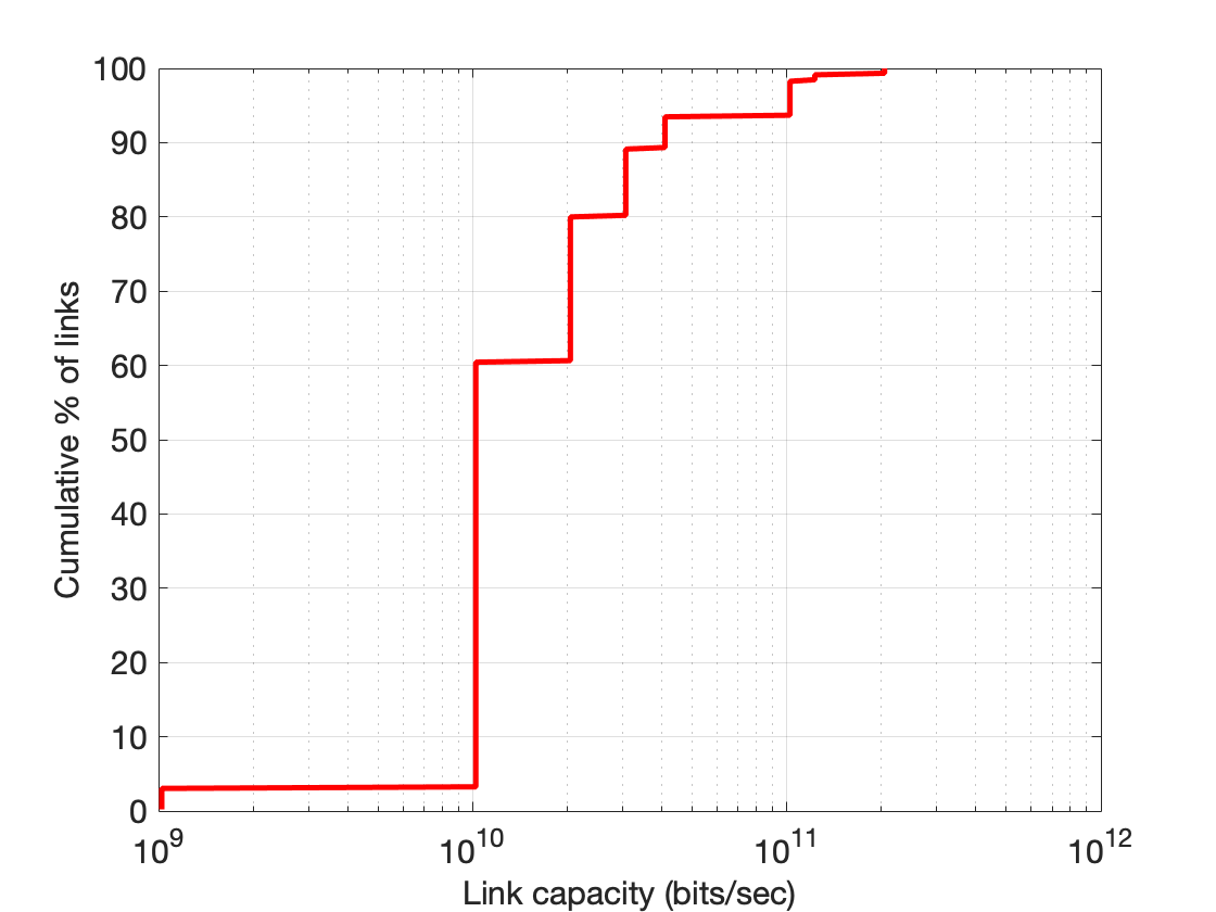
(b) The cumulative distribution function of link capacity.

Figure 5: Illustrations of the total available paths and link capacity.

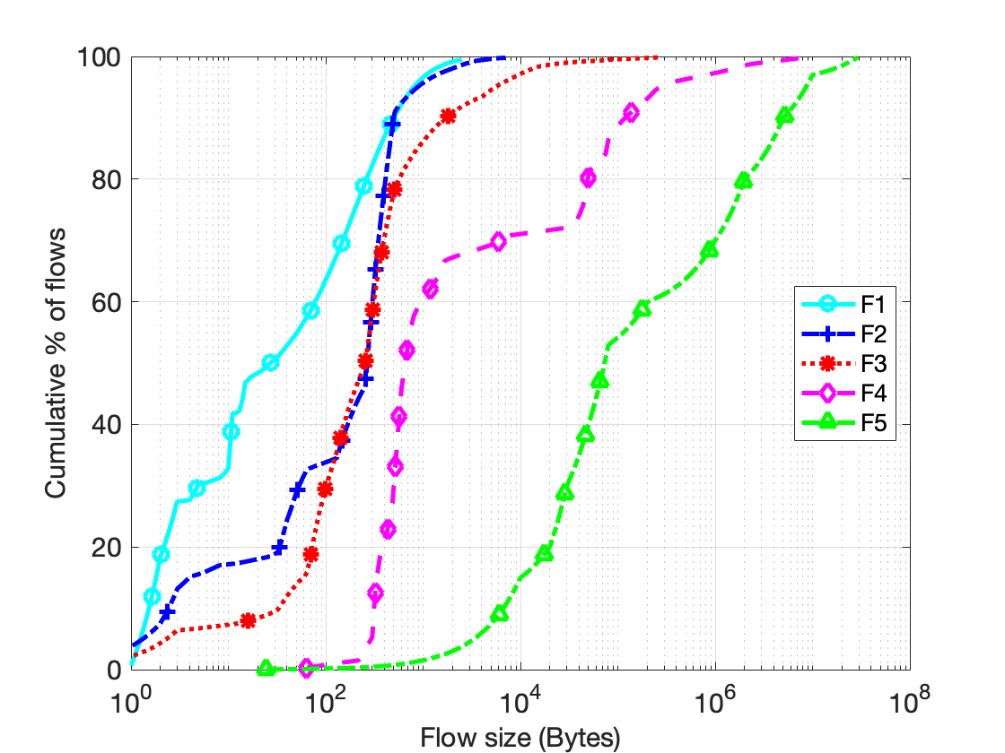
(a) Five types of flow distributions. F1: “FacebookKeyValue_Sampled”; F2: “Google_SearchRPC”; F3: “Google_AllRPC”; F4: “Facebook_HadoopDist_All”; F5: “DCTCP”.

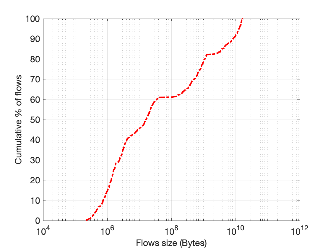
(b) The distribution of our generated flow sizes.

Figure 6: Illustrations of flow distributions.

VI-B Parameter Settings

Our simulation is performed in MATLAB on a PC with an Intel Core i5 at 2.3GHz and 8GB of memory. For the parameters in our objective function, $\alpha$ and $\beta$ are set to be $500$ and $0.05$, respectively. The maximal iteration number is set to be $1500$. In ADMM for the convex scenario of MOPC (4), that is the case when $w_{k}=P_{k},\forall k$, we adjust the parameter $\rho$ according to the Section 3.4.1 in [17], and set the parameter $\mu=1.1\times\rho\|\boldsymbol{R}\|_{2}^{2}$. In the $\boldsymbol{z}$-update, we take an additional step length with $\gamma=1.618$, which demonstrates better convergence performance. The stopping criteria are

• primal residual ($p\_res$):

  $$\|\boldsymbol{y}^{j}-\boldsymbol{Rx}^{j}\|_{2}\leq\sqrt{L}\epsilon^{\text{abs}}+\epsilon^{\text{rel}}\max\{\|\boldsymbol{y}^{j}\|_{2},\|\boldsymbol{R}\boldsymbol{x}^{j}\|_{2}\},$$

• dual residual ($d\_res$):

  $$\|\rho\boldsymbol{R}^{\top}(\boldsymbol{y}^{j}-\boldsymbol{y}^{j-1})\|_{2}\leq\sqrt{P}\epsilon^{\text{abs}}+\epsilon^{\text{rel}}\|\boldsymbol{R}^{\top}\boldsymbol{z}^{j}\|_{2},$$

• constraint violation ($vio$):

  $$\|\max(\boldsymbol{Rx-c},\boldsymbol{0})\|_{2}/\max(\sqrt{L},\|\boldsymbol{c}\|_{2})\leq\epsilon^{tol},$$

where we set $\epsilon^{\text{abs}}=10^{-4},\epsilon^{\text{rel}}=10^{-4}$, and $\epsilon^{\text{tol}}=10^{-10}$.

In ADMM for the non-convex scenario of MOPC (4), that is $\exists k,w_{k}<P_{k}$, due to non-convexity, we increase $\rho$ during the iteration procedure and set $\mu=1.1\times\rho\|\boldsymbol{R}\|_{2}^{2}$. The stopping criteria are

• primal residual ($p\_res$):

  $$\|\boldsymbol{y}^{j}-\boldsymbol{Rx}^{j}\|_{2}/\max(\sqrt{L},\|\boldsymbol{y}^{j}\|_{2})\leq\epsilon^{tol1},$$

• $\boldsymbol{y}$ difference ($y\_dif$):

  $$\|\boldsymbol{y}^{j}-\boldsymbol{y}^{j-1}\|_{2}/\max(\sqrt{L},\|\boldsymbol{y}^{j-1}\|_{2})\leq\epsilon^{tol1},$$

• constraint violation ($vio$):

  $$\|\max(\boldsymbol{Rx-c},\boldsymbol{0})\|_{2}/\max(\sqrt{L},\|\boldsymbol{c}\|_{2})\leq\epsilon^{tol2},$$

where $\epsilon^{tol1}=10^{-4}$, and $\epsilon^{tol2}=10^{-10}$. We utilize

• the total completion time, namely delay,

  $$delay=\sum_{k=1}^{K}\frac{\boldsymbol{s}_{k}}{\|\boldsymbol{x}_{k}\|_{1}},$$

• the proportional fairness,

  $$fairness=\beta\sum_{k=1}^{K}\log(\|\boldsymbol{x}_{k}\|_{1}),$$

• the maximal (say the worst-case) link utilization ratio,

  $$load=\max_{l}\frac{\boldsymbol{R}[l]\boldsymbol{x}}{\boldsymbol{c}_{l}},$$

• the objective function value in MOPC problem,

  $$obj=delay-fairness+\alpha\times load,$$

as performance measures. Next, we present the experimental results in detail.

VI-C Experimental Results

We test several baselines listed in the following:

• $cvxCG$: The conditional gradient method for our original problem (4) without $\ell_{0}$-norm constraints.

• $rlxCG$: The conditional gradient method for the convex relaxation model in (37).

• $cvxCG\_c$: Projecting the solution to $cvxCG$ to meet the $\ell_{0}$-norm constraints.

• $rlxCG\_c$: Projecting the solution to $rlxCG$ to meet the $\ell_{0}$-norm constraints.

• $cvxMOPC$: Our ADMM for our original problem (4) without $\ell_{0}$-norm constraints (because $w_{k}=P_{k},\;\forall k$).

• $ncvMOPC$: Our ADMM for the non-convex problem (4).

As shown in Table I, we verify the advantages of our method. First, the objective function value $obj$ and other three performance measures $delay$, $fairness$, and $load$ in the convex relaxation model $rlxCG$ are nearly the same as those in the original convex model $cvxCG$. Therefore, the convex relaxation technique in [9] does not work in our problem in (4). Second, comparing the results of $cvxCG\_c$ with those of $rlxCG\_c$ shows that there are indeed some improvements of this convex relaxation technique after projecting its solution to meet the path cardinality constraints. In addition, the solution of our non-convex ADMM performs the best compared with other two projected solutions. Figure 7 illustrates the convergence procedure of our non-convex ADMM. It can be observed that our method $ncvMOPC$ gets significant performance gain in $obj$, $delay$ as well as $fairness$ with tiny cost in $load$.

TABLE I: Results of MOPC using ADMM VS convex relaxation.

Scheme	Obj	Delay	Fairness	Load
cvxMOPC	121	329	561	0.70
cvxCG	119	322	564	0.72
rlxCG	119	321	564	0.72
cvxCG_c	391	584	554	0.72
rlxCG_c	369	562	555	0.72
ncvMOPC	169	361	562	0.74

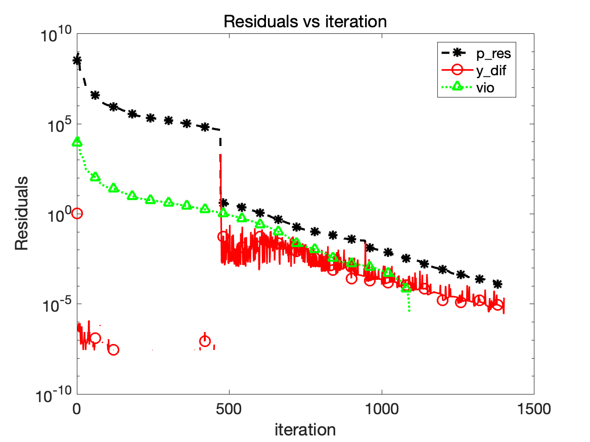
Figure 7: The convergence procedure of our non-convex ADMM for MOPC.

VII Summary

This paper investigates a multi-objective bandwidth optimization and path selection problem for any given path cardinality constraint, which is in general a highly non-convex problem. An ADMM-based algorithm is proposed. The algorithm is simple and easy to be implemented, whose subproblems include finding the maximal root of a single-cubic equation and a one-dimensional optimization problem. We validate the effectiveness of our algorithm both theoretically and experimentally.

Appendix A Proofs

A-A Proof of Lemma 1

Proof.

We reformulate (12) as

$$\boldsymbol{x}^{j+1}_{k}=\mathop{\arg\min}_{\boldsymbol{x}_{k}\geq\boldsymbol{0}}\quad-U_{k}(\sum_{i=1}^{P_{k}}x_{k,i})+\dfrac{\mu}{2}\|\boldsymbol{x}_{k}-\boldsymbol{\nu}_{k}^{j}\|^{2}.$$ (38)

The Lagrangian function of the optimization problem in (38) is

$$L(\boldsymbol{x}_{k};\boldsymbol{\lambda}_{k})=-U_{k}(\sum_{i=1}^{P_{k}}x_{k,i})+\dfrac{\mu}{2}\|\boldsymbol{x}_{k}-\boldsymbol{\nu}_{k}^{j}\|^{2}-\boldsymbol{\lambda}_{k}^{\top}\boldsymbol{x}_{k},$$

where $\boldsymbol{\lambda}_{k}=(\lambda_{k,1},\lambda_{k,2},\cdots,\lambda_{k,P_{k}})^{\top}\geq\boldsymbol{0}$ is a Lagrangian multiplier vector. From the KKT conditions of (38), we can get

$$x_{k,i}^{j+1}=0\quad\text{or}\quad\nu_{k,i}^{j}+\zeta,\quad\forall\,i,$$ (39a)

$$\boldsymbol{x}_{k}^{j+1}\geq\boldsymbol{0},$$ (39b)

$$\mu\zeta=U^{\prime}_{k}\left(\sum_{i=1}^{P_{k}}x_{k,i}^{j+1}\right),$$ (39c)

where $\zeta$ is some positive number. Next, we will show that (39a) and (39b) are actually

$$x_{k,i}^{j+1}=\max(0,\nu_{k,i}^{j}+\zeta),\quad\forall\,i.$$ (40)

Suppose there exists some index $i\,\left(i\in\{1,2,\cdots,P_{k}\}\right)$ such that

$$\nu_{k,i}^{j}+\zeta>0\quad\text{and}\quad x_{k,i}^{j+1}=0.$$

Then the gradient with respect to $\tau$ of the following function

$$-U_{k}(t+\tau)+\frac{\mu}{2}(\tau-\nu_{k,i}^{j})^{2},$$ (41)

where $t$ is the sum of all elements of $\boldsymbol{x}_{k}^{j+1}$ except $x_{k,i}^{j+1}$, in $\tau=0$ is

$$-U_{k}^{\prime}(t+0)+\mu(0-\nu_{k,i}^{j})=-\mu\zeta-\mu\nu_{k,i}^{j}<0.$$

It means that if we increase $x_{k,i}^{j+1}$ from 0, our objective function value would decrease, which contradicts the fact that $x_{k,i}^{j+1}=0$ is optimal. Then we have $x_{k,i}^{j+1}=\nu_{k,i}^{j}+\zeta$, and readily get

$$x_{k,i}^{j+1}=\max(0,\nu_{k,i}^{j}+\zeta),\quad\forall\,i.$$

Combining (39c) with (40) yields

$$\mu\zeta=U^{\prime}_{k}\left(\sum_{i=1}^{P_{k}}\max(0,\nu_{k,i}^{j}+\zeta)\right).$$ (42)

In the following, we will show how to get the value of $\zeta$. Without loss of generality, suppose the elements of $\boldsymbol{\nu}_{k}^{j}$ are in descending order. Since the right hand side of (42) decreases with $\zeta$ increasing and the left hand side increases with $\zeta$ increasing, we can try every positive $\zeta=-\nu_{k,i}^{j}\,(i=2,\cdots,P_{k})$ to determine the corresponding interval in which $\zeta$ satisfies (42). Specifically, if there exists some smallest index $i^{\prime}$ $(i^{\prime}\in{2,\cdots,P_{k}})$ such that

$$\mu\zeta\geq U^{\prime}_{k}\left(\sum_{i=1}^{P_{k}}\max(0,\nu_{k,i}^{j}+\zeta)\right),$$ (43)

where $\zeta=-\nu_{k,i^{\prime}}^{j}$, then the corresponding interval is $(-\nu_{k,i^{\prime}-1}^{j},-\nu_{k,i^{\prime}}^{j}]$. The corresponding interval is $(-\nu^{j}_{k,P_{k}},+\infty)$ otherwise. Then, we can obtain $\zeta$ through finding the maximal root of a single-variable cubic equation

$$\mu\zeta\left(\sum_{i=1}^{i^{\prime}-1}(\nu^{j}_{k,i}+\zeta)\right)^{2}=\beta\left(\sum_{i=1}^{i^{\prime}-1}(\nu^{j}_{k,i}+\zeta)\right)+s_{k},$$

or

$$\mu\zeta\left(\sum_{i=1}^{P_{k}}(\nu^{j}_{k,i}+\zeta)\right)^{2}=\beta\left(\sum_{i=1}^{P_{k}}(\nu^{j}_{k,i}+\zeta)\right)+s_{k},$$

otherwise.

∎

A-B Proof of Lemma 2

Proof.

If $w_{k}=1$, $\boldsymbol{x}_{k}^{j+1}$ can have one and only one non-zero element. Next, we would first show the index of this non-zero element and then determine its corresponding value. Suppose there exist $i,i^{\prime}\,(i,i^{\prime}\in\{1,\cdots,P_{k}\})$ such that $\nu_{k,i^{\prime}}^{j}<\nu_{k,i}^{j}$, then for $\forall a>0$, we have

$$-U_{k}(a)+\frac{\mu}{2}(a-\nu_{k,i^{\prime}}^{j})^{2}+\frac{\mu}{2}(\nu_{k,i}^{j})^{2}$$

$$>-U_{k}(a)+\frac{\mu}{2}(a-\nu^{j}_{k,i})^{2}+\frac{\mu}{2}(\nu^{j}_{k,i^{\prime}})^{2},$$

meaning that $(\overbrace{0,\cdot\cdot\cdot,0}^{i^{\prime}-1},a,0,\cdot\cdot\cdot,0)^{\top}$ is less optimal than $(\overbrace{0,\cdot\cdot\cdot,0}^{i-1},a,0,\cdot\cdot\cdot,0)^{\top}$. Hence, the index of the non-zero element is $i$ $(i\in\{1,\cdots,P_{k}\})$ that makes $\nu^{j}_{k,i}$ be maximal. Now problem (22) is converted into a single-variable optimization problem:

$$x^{j+1}_{k,i} =\mathop{\arg\min}_{a}-U_{k}(a)+\dfrac{\mu}{2}(a-\nu^{j}_{k,i})^{2}.$$ (44)

To make the gradient of problem (44) be zero, we obtain a single-variable cubic equation

$$\mu a^{3}-\mu\nu^{j}_{k,i}a^{2}-\beta a-s_{k}/K=0,\quad\forall k.$$

$x_{k,i}^{j+1}$ is the maximal real positive root (there is at least one real positive root because $-s_{k}/K<0$). ∎

A-C Proof of Lemma 3

Proof.

First, when $1<w_{k}<P_{k}$, we prove the solution to (22) satisfies that if $i>w_{k}$, $x_{k,i}^{j+1}=0$ by contradiction.

Suppose one solution $\tilde{\boldsymbol{x}}_{k}^{j+1}$ satisfies that there exists $i>w_{k}$ such that $\tilde{x}_{k,i}^{j+1}=d>0$, then there exists $i^{\prime}\leq w_{k}$ such that $\tilde{x}_{k,i^{\prime}}^{j+1}=0$, i.e.

$$\tilde{\boldsymbol{x}}_{k}^{j+1}=(\tilde{x}_{k,1}^{j+1},\cdots,{\tilde{x}_{k,i^{\prime}}^{j+1}=0},\cdots,{\tilde{x}_{k,i}^{j+1}=d},\cdots,\tilde{x}_{k,P_{k}}^{j+1})^{\top}.$$

We can construct another feasible point by switching the values of $\tilde{x}_{k,i^{\prime}}^{j+1}$ and $\tilde{x}_{k,i}^{j+1}$. Then we get

$$\hat{\boldsymbol{x}}_{k}^{j+1}=(\tilde{x}_{k,1}^{j+1},\cdots,{\hat{x}_{k,i^{\prime}}^{j+1}=d},\cdots,{\hat{x}_{k,i}^{j+1}=0},\cdots,\tilde{x}_{k,P_{k}}^{j+1})^{\top}.$$

Because of $\nu^{j}_{k,i}\leq\nu^{j}_{k,i^{\prime}}$, we have

$$-U_{k}(t+d)+\frac{\mu}{2}(d-\nu^{j}_{k,i^{\prime}})^{2}+\frac{\mu}{2}(\nu^{j}_{k,i})^{2}$$

$$\leq-U_{k}(t+d)+\frac{\mu}{2}(\nu^{j}_{k,i^{\prime}})^{2}+\frac{\mu}{2}(d-\nu^{j}_{k,i})^{2},$$

where $t$ is the sum of all elements of $\boldsymbol{x}_{k}^{j+1}$ except $x_{k,i}^{j+1}$ and $x_{k,i^{\prime}}^{j+1}$. Hence, $\hat{\boldsymbol{x}}_{k}^{j+1}$ is better than $\tilde{\boldsymbol{x}}_{k}^{j+1}$. By repeating this procedure, we get our conclusion $x_{k,i}^{j+1}=0,\;i>w_{k}$.

Now problem (22) can be transformed to

$$(x^{j+1}_{k,1},\cdots,x^{j+1}_{k,w_{k}})^{\top}=$$

$$\mathop{\arg\min}_{x_{k,i}\geq 0,i\leq w_{k}}\quad-U_{k}(\sum_{i=1}^{w_{k}}x_{k,i})+\dfrac{\mu}{2}\sum_{i=1}^{w_{k}}(x_{k,i}-\nu^{j}_{k,i})^{2}.$$ (45)

From similar analysis in the proof of lemma 1, the solution to (45) satisfies (24a) and (24b). This completes the proof.

∎

A-D Proof of Lemma 4

Proof.

Consider problem (27). For a fixed $t$, the optimal $\boldsymbol{y}$ is shown in (29). If $t^{*}$ is the optimal solution to

$$\min_{t}\Phi(t)=\phi(t,\boldsymbol{y}(t))\quad s.t.\quad t\geq 0,$$

then $\boldsymbol{y}(t^{*})$ is the optimal solution to problem (19) (since for any other feasible $t^{\prime}$ and $\boldsymbol{y}^{\prime}$, we have

$$\phi(t^{\prime},\boldsymbol{y}^{\prime})\geq\phi(t^{\prime},\boldsymbol{y}(t^{\prime}))=\Phi(t^{\prime})\geq\Phi(t^{*})=\phi(t^{*},\boldsymbol{y}(t^{*})).$$

By noticing that the function

$$\Phi(t)=\phi(t,\boldsymbol{y}(t))=\inf_{\boldsymbol{y}\in\mathcal{C}}\,\phi(t,\boldsymbol{y}),$$

is convex in $t$ (because $\phi$ is convex in $(t,\boldsymbol{y})$, and $\mathcal{C}$ is a convex nonempty set), and when $t>1$, $\Phi(t)$ will increase. This concludes the proof. ∎

A-E Proof of Proposition 1

Proof.

We recast the augmented Lagrangian function (31) into another form:

$$L_{\rho}(\boldsymbol{x}^{j},\boldsymbol{y}^{j};\boldsymbol{z}^{j})=f(\boldsymbol{x}^{j})+g(\boldsymbol{y}^{j})+\mathcal{I}_{\mathcal{X}}(\boldsymbol{x}^{j})+\mathcal{I}_{\mathcal{Y}}(\boldsymbol{y}^{j})$$

$$+\frac{\rho}{2}\|\boldsymbol{y}^{j}-\boldsymbol{R}\boldsymbol{x}^{j}+\frac{\boldsymbol{z}^{j}}{\rho}\|^{2}-\frac{\|\boldsymbol{z}^{j}\|^{2}}{2\rho}.$$

Since when $\boldsymbol{x}^{j}_{k,i}\rightarrow\infty\,(k\in\{1,2,\cdots,K\},\forall i\in\{1,2,\cdots,P_{k}\})$, we have $\|\boldsymbol{Rx}^{j}\|\rightarrow+\infty$, which combining with the boundedness of $\{\boldsymbol{y}^{j}\}$ and $\{\boldsymbol{z}^{j}\}$ implies that $f(\boldsymbol{x}^{j})+\frac{\rho}{2}\|\boldsymbol{y}^{j}-\boldsymbol{R}\boldsymbol{x}^{j}+\frac{\boldsymbol{z}^{j}}{\rho}\|^{2}\rightarrow+\infty$. Besides, other parts of $L_{\rho}(\boldsymbol{x}^{j},\boldsymbol{y}^{j};\boldsymbol{z}^{j})$ are all bounded below. We get the lower boundedness of $\{L_{\rho}(\boldsymbol{x}^{j},\boldsymbol{y}^{j};\boldsymbol{z}^{j})\}$. ∎

A-F Proof of Lemma 5

Proof.

For simplicity, we denote $h(\boldsymbol{x})=\frac{\rho}{2}\|\boldsymbol{y}^{j}-\boldsymbol{Rx}+\boldsymbol{z}^{j}/\rho\|^{2}$, then the $\boldsymbol{x}$-update (21) is actually

$$\boldsymbol{x}^{j+1}=\mathop{\arg\min}_{\boldsymbol{x}\in\mathcal{X}}f(\boldsymbol{x})+\langle\nabla h(\boldsymbol{x}^{j}),\boldsymbol{x}-\boldsymbol{x}^{j}\rangle+\frac{\mu}{2}\|\boldsymbol{x}-\boldsymbol{x}^{j}\|^{2},$$

which yields that

$$f(\boldsymbol{x}^{j})\geq$$

$$f(\boldsymbol{x}^{j+1})+\langle\nabla h(\boldsymbol{x}^{j}),\boldsymbol{x}^{j+1}-\boldsymbol{x}^{j}\rangle+\frac{\mu}{2}\|\boldsymbol{x}^{j+1}-\boldsymbol{x}^{j}\|^{2}.$$ (46)

Since $\|\nabla h(\boldsymbol{x})-\nabla h(\boldsymbol{x}^{\prime})\|\leq\rho\|\boldsymbol{R}\|_{2}^{2}\|\boldsymbol{x}-\boldsymbol{x}^{\prime}\|,\forall\boldsymbol{x},\boldsymbol{x}^{\prime}$, from Lemma 1 in [22], we have

$$h(\boldsymbol{x}^{j+1})\leq h(\boldsymbol{x}^{j})$$

$$+\langle\nabla h(\boldsymbol{x}^{j}),\boldsymbol{x}^{j+1}-\boldsymbol{x}^{j}\rangle+\frac{\rho\|\boldsymbol{R}\|_{2}^{2}}{2}\|\boldsymbol{x}^{j+1}-\boldsymbol{x}^{j}\|^{2}.$$ (47)

Summing up (46) and (47) gives

$$L_{\rho}(\boldsymbol{x}^{j},\boldsymbol{y}^{j};\boldsymbol{z}^{j})-L_{\rho}(\boldsymbol{x}^{j+1},\boldsymbol{y}^{j};\boldsymbol{z}^{j})$$

$$=f(\boldsymbol{x}^{j})+h(\boldsymbol{x}^{j})-f(\boldsymbol{x}^{j+1})-h(\boldsymbol{x}^{j+1})$$

$$\geq\frac{\mu-\rho\|\boldsymbol{R}\|_{2}^{2}}{2}\|E_{\boldsymbol{x}}^{j+1}\|^{2}.$$ (48)

The $\boldsymbol{y}$-update (19) is

$$\boldsymbol{y}^{j+1}=\mathop{\arg\min}_{\boldsymbol{0}\leq\boldsymbol{y}\leq\boldsymbol{c}}g(\boldsymbol{y})+\dfrac{\rho}{2}\|\boldsymbol{y}-\boldsymbol{Rx}^{j+1}+\boldsymbol{z}^{j}/\rho\|^{2},$$

whose optimality condition deduces that $\exists\,\boldsymbol{g}^{j+1}\in\partial g(\boldsymbol{y}^{j+1})$ such that

$$\left(\boldsymbol{g}^{j+1}+\rho(\boldsymbol{y}^{j+1}-\boldsymbol{Rx}^{j+1}+\boldsymbol{z}^{j}/\rho)\right)^{\top}(\boldsymbol{y}^{\prime}-\boldsymbol{y}^{j+1})\geq 0,$$ (49)

where $\boldsymbol{0}\leq\boldsymbol{y}^{\prime}\leq\boldsymbol{c}$. Then we have

$$L_{\rho}(\boldsymbol{x}^{j+1},\boldsymbol{y}^{j};\boldsymbol{z}^{j})-L_{\rho}(\boldsymbol{x}^{j+1},\boldsymbol{y}^{j+1};\boldsymbol{z}^{j})$$

$$=g(\boldsymbol{y}^{j})-g(\boldsymbol{y}^{j+1})$$

$$+\frac{\rho}{2}\|\boldsymbol{y}^{j}-\boldsymbol{Rx}^{j+1}+\boldsymbol{z}^{j}/\rho\|^{2}-\frac{\rho}{2}\|\boldsymbol{y}^{j+1}-\boldsymbol{Rx}^{j+1}+\boldsymbol{z}^{j}/\rho\|^{2}$$

$$=g(\boldsymbol{y}^{j})-g(\boldsymbol{y}^{j+1})$$

$$+\frac{\rho}{2}\|\boldsymbol{y}^{j}-\boldsymbol{y}^{j+1}\|^{2}+\rho\langle\boldsymbol{y}^{j+1}-\boldsymbol{Rx}^{j+1}+\boldsymbol{z}^{j}/\rho,\boldsymbol{y}^{j}-\boldsymbol{y}^{j+1}\rangle$$

$$\geq(\boldsymbol{g}^{j+1})^{\top}(\boldsymbol{y}^{j}-\boldsymbol{y}^{j+1})$$

$$+\frac{\rho}{2}\|\boldsymbol{y}^{j}-\boldsymbol{y}^{j+1}\|^{2}+\rho\langle\boldsymbol{y}^{j+1}-\boldsymbol{Rx}^{j+1}+\boldsymbol{z}^{j}/\rho,\boldsymbol{y}^{j}-\boldsymbol{y}^{j+1}\rangle$$

$$\overset{\eqref{eq: convergeopt}}{\geq}\frac{\rho}{2}\|E_{\boldsymbol{y}}^{j+1}\|^{2},$$ (50)

where the second equality is derived from

$$\|\boldsymbol{v}\|^{2}-\|\boldsymbol{w}\|^{2}=\|\boldsymbol{v}-\boldsymbol{w}\|^{2}+2\langle\boldsymbol{w},\boldsymbol{v}-\boldsymbol{w}\rangle,\;\forall\boldsymbol{v},\boldsymbol{w}\in\mathbb{R}^{L}.$$

For the $\boldsymbol{z}$-update, we have

$$L_{\rho}(\boldsymbol{x}^{j+1},\boldsymbol{y}^{j+1};\boldsymbol{z}^{j})-L_{\rho}(\boldsymbol{x}^{j+1},\boldsymbol{y}^{j+1};\boldsymbol{z}^{j+1})$$

$$=(\boldsymbol{z}^{j}-\boldsymbol{z}^{j+1})^{\top}(\boldsymbol{y}^{j+1}-\boldsymbol{Rx}^{j+1})$$

$$=-\frac{1}{\rho}\|E_{\boldsymbol{z}}^{j+1}\|^{2}.$$ (51)

By summing up (48), (50), and (51), we complete the proof. ∎

A-G Proof of Theorem 1

Proof.

From $\sum_{j=1}^{\infty}\|E_{\boldsymbol{z}}^{j+1}\|^{2}<\infty$, we can get $\lim\limits_{j\rightarrow+\infty}E_{\boldsymbol{z}}^{j+1}=\boldsymbol{0}$. Next, we first show that

$$\lim\limits_{j\rightarrow+\infty}E_{\boldsymbol{x}}^{j+1}=\boldsymbol{0}\;\text{and}\;\lim\limits_{j\rightarrow+\infty}E_{\boldsymbol{y}}^{j+1}=\boldsymbol{0}.$$ (52)

Since $\{L_{\rho}(\boldsymbol{x}^{j},\boldsymbol{y}^{j};\boldsymbol{z}^{j})\}$ is bounded below and $\sum_{j=1}^{\infty}\|E_{\boldsymbol{z}}^{j+1}\|^{2}<\infty$, it follows from (36) that

$$\sum_{j=1}^{\infty}\|E_{\boldsymbol{x}}^{j+1}\|^{2}<\infty,\,\sum_{j=1}^{\infty}\|E_{\boldsymbol{y}}^{j+1}\|^{2}<\infty,$$ (53)

which implies (52). The boundedness of $\{\boldsymbol{x}^{j}\}_{j=1}^{+\infty}$ can be obtained from the boundedness of $\{\boldsymbol{y}^{j}\}_{j=1}^{+\infty}$, $\{\boldsymbol{z}^{j}\}_{j=1}^{+\infty}$ as well as the $\boldsymbol{z}$-update in (20). In addition, because of the $\boldsymbol{z}$-update in (20), we can have

$$\lim\limits_{j\rightarrow\infty}\boldsymbol{y}^{j}-\boldsymbol{R}\boldsymbol{x}^{j}=0.$$ (54)

For any limiting point $\{\overline{\boldsymbol{x}},\overline{\boldsymbol{y}}\}$ of the sequence, since $\{\boldsymbol{x}^{j},\boldsymbol{y}^{j},\boldsymbol{z}^{j}\}$ is bounded, there is a sequence $\{\boldsymbol{x}^{j_{i}},\boldsymbol{y}^{j_{i}},\boldsymbol{z}^{j_{i}}\}$ whose limiting point is $\{\overline{\boldsymbol{x}},\overline{\boldsymbol{y}},\overline{\boldsymbol{z}}\}$. Clearly, from (54), we can get

$$\overline{\boldsymbol{y}}=\boldsymbol{R}\overline{\boldsymbol{x}},$$

which is in fact (32c) in KKT conditions. Taking limit on both sides of (33), (35) and applying the Remark 1 in [22], we obtain (32a), (32b) in the KKT conditions. ∎

References

- [1] J. Kimball, T. Wypych, and F. Kuester, “Low bandwidth desktop and video streaming for collaborative tiled display environments,” Future Gener. Comput. Syst., vol. 54, pp. 336–343, 2016.
- [2] K. Lee, D. Chu, E. Cuervo, J. Kopf, Y. Degtyarev, S. Grizan, A. Wolman, and J. Flinn, “Outatime: Using speculation to enable low-latency continuous interaction for mobile cloud gaming,” in Proc. Annu. Int. Conf. Mobile Syst., Appl., Services (MobiSys), 2015, pp. 151–165.
- [3] M. S. Elbamby, C. Perfecto, M. Bennis, and K. Doppler, “Toward low-latency and ultra-reliable virtual reality,” IEEE Netw., vol. 32, no. 2, pp. 78–84, 2018.
- [4] C. Tian, A. Munir, A. X. Liu, Y. Liu, Y. Li, J. Sun, F. Zhang, and G. Zhang, “Multi-tenant multi-objective bandwidth allocation in datacenters using stacked congestion control,” in Proc. IEEE Conf. Comput. Commun. (INFOCOM), 2017, pp. 1–9.
- [5] Y. Wang, J. Zheng, L. Tan, and C. Tian, “Joint optimization on bandwidth allocation and route selection in qoe-aware traffic engineering,” IEEE Access, vol. 7, pp. 3314–3319, 2018.
- [6] J. Perry, A. Ousterhout, H. Balakrishnan, D. Shah, and H. Fugal, “Fastpass: a centralized” zero-queue” datacenter network,” in Proc. ACM Conf. SIGCOMM, 2014, pp. 307–318.
- [7] K. Nagaraj, D. Bharadia, H. Mao, S. Chinchali, M. Alizadeh, and S. Katti, “Numfabric: Fast and flexible bandwidth allocation in datacenters,” in Proc. ACM Conf. SIGCOMM, 2016, pp. 188–201.
- [8] M. Grant and S. Boyd, “Cvx: Matlab software for disciplined convex programming, version 2.1,” 2014.
- [9] Y. Bi, C. W. Tan, and A. Tang, “Network utility maximization with path cardinality constraints,” in Proc. IEEE Conf. Comput. Commun. (INFOCOM), 2016, pp. 1–9.
- [10] C. Xu, L. Tao, H. Wu, D. Ye, and G. Zhang, “Multiple constrained routing algorithms in large-scaled software defined networks,” CoRR, vol. abs/1902.10312, 2019.
- [11] K. Papagiannaki, S. Moon, C. Fraleigh, P. Thiran, and C. Diot, “Measurement and analysis of single-hop delay on an ip backbone network,” IEEE J. Sel. Areas Commun., vol. 21, no. 6, pp. 908–921, 2003.
- [12] Y. Feng, B. Li, and B. Li, “Airlift: Video conferencing as a cloud service using inter-datacenter networks,” in Proc. 20th IEEE Int. Conf. Netw. Protocols (ICNP), 2012, pp. 1–11.
- [13] Y. Cao, M. Xu, and X. Fu, “Delay-based congestion control for multipath tcp,” in Proc. 20th IEEE Int. Conf. Netw. Protocols (ICNP), 2012, pp. 1–10.
- [14] F. P. Kelly, A. K. Maulloo, and D. K. Tan, “Rate control for communication networks: shadow prices, proportional fairness and stability,” J. Oper. Res. Soc., vol. 49, no. 3, pp. 237–252, 1998.
- [15] R. Gupta, L. Vandenberghe, and M. Gerla, “Centralized network utility maximization over aggregate flows,” in Proc. 14th Int. Symp. Modeling Optim. Mobile, Ad Hoc, Wireless Netw. (WiOpt), 2016, pp. 1–8.
- [16] Z. Allybokus, K. Avrachenkov, J. Leguay, and L. Maggi, “Multi-path alpha-fair resource allocation at scale in distributed software-defined networks,” IEEE J. Sel. Areas Commun., vol. 36, no. 12, pp. 2655–2666, 2018.
- [17] S. Boyd, N. Parikh, E. Chu, B. Peleato, and J. Eckstein, “Distributed optimization and statistical learning via the alternating direction method of multipliers,” Found. Trends Mach. Learn., vol. 3, no. 1, pp. 1–122, 2011.
- [18] G. E. Forsythe, M. A. Malcolm, and C. B. Moler, Computer methods for mathematical computations. Prentice-Hall Englewood Cliffs, NJ, 1976.
- [19] R. P. Brent, Algorithms for minimization without derivatives. Prentice-Hall Englewood Cliffs, NJ, 1973.
- [20] L. Chen, D. Sun, and K.-C. Toh, “A note on the convergence of admm for linearly constrained convex optimization problems,” Comput. Optim. Appl., vol. 66, no. 2, pp. 327–343, 2017.
- [21] H. Attouch, J. Bolte, and B. F. Svaiter, “Convergence of descent methods for semi-algebraic and tame problems: proximal algorithms, forward–backward splitting, and regularized gauss–seidel methods,” Math. Program. A, vol. 137, no. 1-2, pp. 91–129, 2013.
- [22] J. Bolte, S. Sabach, and M. Teboulle, “Proximal alternating linearized minimization for nonconvex and nonsmooth problems,” Math. Program., vol. 146, no. 1-2, pp. 459–494, 2014.
- [23] M. Jaggi, “Revisiting frank-wolfe: Projection-free sparse convex optimization.” in Proc. Int. Conf. Mach. Learn. (ICML), 2013, pp. 427–435.
- [24] B. Montazeri, Y. Li, M. Alizadeh, and J. Ousterhout, “Homa: A receiver-driven low-latency transport protocol using network priorities,” in Proc. ACM Conf. SIGCOMM, 2018, pp. 221–235.