Dynamical spectral structure of density fluctuation near QCD critical point

Abstract

The expression for the dynamical spectral structure of the density fluctuation near the QCD critical point has been derived using linear response theory within the purview of Israel-Stewart relativistic viscous hydrodynamics. The change in spectral structure of the system as it moves toward critical end point has been studied. The effects of the critical point have been introduced in the system through a realistic equation of state and the scaling behaviour of various transport coefficients and thermodynamic response functions. We have found that the Brillouin and the Rayleigh peaks are distinctly visible when the system is away from critical point but the peaks tend to merge near the critical point. The sensitivity of structure of the spectral function on wave vector ($k$) of the sound wave has been demonstrated. It has been shown that the Brillouin peaks get merged with the Rayleigh peak because of the absorption of sound waves in the vicinity of the critical point.

I Introduction

Relativistic Heavy Ion Collisions experiments (RHIC-E) are aimed at exploring properties of high temperature Cabibbo:1975ig and high density Collins:1974ky state of strongly interacting matter. The degrees of freedom of hadronic matter under extreme conditions of temperature and density are deconfined quarks and gluons and their interaction is governed by Quantum Chromodynamics (QCD). The study of the deconfined state of strongly interacting matter is relevant for understanding the evolution of micro-second old universe, composition of the core of the compact astrophysical objects (e.g. neutron star) and properties of non-abelian gauge theory in medium qgp1 ; qgp2 . The RHIC-E provide opportunities to verify different theoretical predictions on the thermal nature of QCD matter Busza:2018rrf . Results of these experiments indicate that after collision of two heavy ions at relativistic energies, a strongly interacting perfect fluid medium consisting of quarks and gluons - called quark gluon plasma (QGP) ShuryakPhysRep - is formed npa2005 . The fluid with high internal pressure expands hydrodynamically, cools consequently and revert to hadronic phase. The thermal properties of the QGP can be described by two independent variables, the temperature ($T$) and baryonic chemical potential ($\mu$) associated with the conservation of net baryon number in the system. The values of $T$ and $\mu$ of the system depends on the energy of collisions of the nuclei. Numerical simulation of QCD in the high $T$ and low $\mu$ $(\rightarrow 0)$ region predict that the quark-hadron transition is a cross-over  Fodor:2001pe ; Asakawa:1989bq ; Halasz:1998qr ; deForcrand:2002hgr ; Aoki:2006we . However, calculations based on several QCD inspired models indicate that at high $\mu$ region the transition is first order deForcrand:2002hgr ; Endrodi:2011gv . Therefore, it is expected that between the cross over and first order transitions there exists a region or point in $T-\mu$ plane where the first order transition ends and crossover begins Fodor:2004nz . This point is the QCD Critical End Point(CEP). At present, lattice QCD results for high $\mu$ is not available due to the well known sign problem for spin 1/2 particles. As a result the prediction on the precise position of the CEP is not possible from first principle calculations Gavai:2014ela . Due to the lack of first principle calculations there have been a large numbers of effective field theory based studies on the QCD phase at non-zero baryon density  PNJL10 ; PNJL11 ; PNJL12 ; PQM1 ; PQM2 ; PQM3 . These model studies indicate the existence of CEP in the phase diagram. However, the position of the CEP is still ambiguous as its location depends on the parameters of the models used.

Different points of the QCD phase diagram in the $\mu-T$ plane can be reached experimentally by varying the energy of the colliding nuclei. The deconfined, i.e the QGP systems with different $T$ and $\mu$ can be produced by colliding heavy ions with different energies. These systems will follow different trajectories in $\mu-T$ plane while making a transition from QGP to hadrons due to cooling caused by expansion. Parallel to the theoretical endeavor, experimental efforts are on to explore these trajectories passing through/near the CEP by varying beam energy Aggarwal:2010cw .

It is well-known that the density-density correlation length diverges at the critical point. The effects of the divergence on the baryon number fluctuations, particle correlations and correlations of density fluctuations will have better chance to be detected provided the fluctuation survives the hadronic evolution. It is important to understand the correlations of these fluctuations theoretically for identifying signatures of CEP in data. The fluid dynamical descriptions of the system at the CEP breaks down. However, it is possible to identify a region near the CEP where the fluid dynamics remains valid and can be used to understand the properties of the system Stanley . The effects of CEP on the evolution of matter goes as input through the equation of state (EoS) and via the critical behaviour of the transport coefficients and response functions of the fluid.

The correlation of density fluctuations can be investigated through the spectral structure ($\mathscr{S}_{nn}(\mathchoice{\mbox{\boldmath$k$}}{\mbox{\boldmath$k$}}{\mbox{\boldmath$\scriptstyle k$}}{\mbox{\boldmath$\scriptscriptstyle k$}},\omega)$) in Fourier space near the CEP. Spectral function has been studied experimentally in the condensed matter physics laboratories to estimate the speed of sound by using scattering of light. The position of Brillouin peaks (B-Peaks) in the $\mathscr{S}_{nn}(\mathchoice{\mbox{\boldmath$k$}}{\mbox{\boldmath$k$}}{\mbox{\boldmath$\scriptstyle k$}}{\mbox{\boldmath$\scriptscriptstyle k$}},\omega)$ is connected to the speed of sound and various transport coefficients like thermal conductivity, shear and bulk viscosities and response functions like specific heats. Sadly, such external probes are not available to examine the properties of QCD matter near CEP.

The spectral structure has been estimated in Ref. kunihiro but the effects of EoS containing the critical point have been ignored. It has been shown in that work that the EoS plays a vital role in determining the behaviour of $\mathscr{S}_{nn}(\mathchoice{\mbox{\boldmath$k$}}{\mbox{\boldmath$k$}}{\mbox{\boldmath$\scriptstyle k$}}{\mbox{\boldmath$\scriptscriptstyle k$}},\omega)$, especially its strength at the Rayleigh peak (R-peak) changes by several orders of magnitude if EoS with effects of CEP is incorporated. The EoS has strong effects on B-peak too. It is also very important to understand whether all the hydrodynamic modes travel with the same speed or not. The R-peak and the B-peaks will be closer for slower modes even at points away from the CEP. Therefore, the structure of $\mathscr{S}_{nn}(\mathchoice{\mbox{\boldmath$k$}}{\mbox{\boldmath$k$}}{\mbox{\boldmath$\scriptstyle k$}}{\mbox{\boldmath$\scriptscriptstyle k$}},\omega)$ will shed light on the speed of the perturbation propagating as sound wave.

The paper is organized as follows. The EoS containing the effects of CEP is discussed in the next section. The expression for $\mathscr{S}_{nn}(\mathchoice{\mbox{\boldmath$k$}}{\mbox{\boldmath$k$}}{\mbox{\boldmath$\scriptstyle k$}}{\mbox{\boldmath$\scriptscriptstyle k$}},\omega)$ has been derived in section III within the scope of the Israel-Stewart (IS) relativistic hydrodynamics in Eckart frame of reference. Section IV is devoted to discuss the critical behaviour of some transport coefficients and response functions. Results are presented in section VI and section VII is dedicated to summary and discussions.

II Equation of State

One of our main objectives is to investigate the role of the CEP on the density fluctuation. In order to observe it, we have constructed an EoS  mitedu ; nonaka ; hasan which contains the effects of CEP. To make the article self-contained, we here briefly discuss the construction of the EoS. The universality hypothesis suggests that the 3D Ising model and the QCD belong to the same universality class. Therefore, we can map the calculation of 3D Ising model onto the QCD phase diagram. It is well-known that magnetization $(M)$ of Ising model is analogous to a critical entropy density ($s_{c}$) in QCD. We can express $M$ at any temperature $(T)$ as a function of reduced temperature, $r=(T-T_{c})/T_{c}$ and applied magnetic field $(\mathscr{H})$, where $T_{c}$ is the critical temperature, with the location of CEP at $(r,\mathscr{H})=(0,0)$. Thus, $r<0$ represents the first order phase transition and $r>0$ indicates the crossover transition. A linear mapping between CEP of Ising model and CEP of QCD phase diagram is performed by assuming a critical region by the following relation

$$r=\frac{T-T_{c}}{\Delta T_{c}},\,\,\,\,\mathscr{H}=\frac{\mu-\mu_{c}}{\Delta\mu_{c}}$$ (1)

where $(\mu_{c},T_{c})$ represents the location of the CEP in the QCD phase diagram. The extension of the critical region can be determined by the values of $\Delta T_{c}$ and $\Delta\mu_{c}$ where $\Delta T_{c}$ and $\Delta\mu_{c}$ are chosen as extensions of the critical region along T and $\mu$ axis respectively. The critical entropy density can be expressed as

$$s_{c}=\frac{M(r,\mathscr{H})}{\Delta T_{c}}=M\Big{(}\frac{T-T_{c}}{\Delta T_{c}},\frac{\mu-\mu_{c}}{\Delta\mu_{c}}\Big{)}\frac{1}{\Delta T_{c}}$$ (2)

In order to construct the EoS, we first construct a dimensionless entropy density as

$$S_{c}=A(\Delta T_{c},\Delta\mu_{c})s_{c}(T,\mu)$$ (3)

when $A$ is defined as

$$A(\Delta T_{c},\Delta\mu_{c})=B\sqrt{\Delta T^{2}_{c}+\Delta\mu_{c}^{2})}$$ (4)

Here $B$ is also a dimensionless quantity which represents the elongation of the critical region. In this work, we use $(T_{c},\mu_{c})=(154\text{MeV},367\text{MeV})$ with $(\Delta T_{c},\Delta\mu_{c},B)=(0.1\,\text{GeV},0.2\,\text{GeV},2)$. The construction of the entropy density is done by making a correspondence between the entropy density of QGP ($s_{Q}$) and the hadronic ($s_{H}$) phases with use of $S_{c}$ as a switching function. The final result reads

$$S(T,\mu)=\frac{1}{2}[1-{\rm tanh}\ S_{c}(T,\mu)]s_{Q}(T,\mu)+\frac{1}{2}[1+{\rm tanh}\ S_{c}(T,\mu)]s_{H}(T,\mu)$$ (5)

where we calculate $s_{Q}$ assatarov

$$s_{Q}(T,\mu)=\frac{32+21N_{f}}{45}\pi^{2}T^{3}+\frac{N_{f}}{9}\mu^{2}T$$ (6)

with $N_{f}$ being the number of flavor of quarks.
The hadronic entropy density ($s_{H}$) can be estimated from the following expression  pbraun ; Sarwar ,

$$s_{H}(T,\mu)=\pm\sum_{i}\frac{g_{i}}{2\pi^{2}}\int^{\infty}_{0}dp^{\prime}{p^{\prime}}^{2}\Big{[}ln\Big{(}1\pm\{exp(E_{i}-\mu_{i})/T\}\Big{)}\pm\frac{E_{i}-\mu_{i}}{T\{exp(E_{i}-\mu_{i})/T\pm 1\}}\Big{]}$$ (7)

where the sum extends over all hadrons with mass up to 2.5 GeV Sarwar , $g_{i}$ represents the statistical degeneracy factor and $E_{i}=\sqrt{{p^{\prime}}^{2}_{i}+m^{2}_{i}}$ is the energy of the $i^{\text{th}}$ hadron.

Once we know the entropy density, the thermodynamic quantities e.g. baryon number density, pressure and energy density can be evaluated as follows. The net baryon number density ($n$) is given by

$$n(T,\mu)=\int_{0}^{T}\frac{\partial S(T^{{}^{\prime}},\mu)}{\partial\mu}dT^{{}^{\prime}}$$ (8)

The pressure can be estimated as

$$p(T,\mu)=\int_{0}^{T}S(T^{{}^{\prime}},\mu)dT^{{}^{\prime}}$$ (9)

and finally, the energy density is given by,

$$\epsilon(T,\mu)=Ts(T,\mu)-p(T,\mu)+\mu n$$ (10)

To get the first order phase boundary, the discontinuity in the entropy density along the transition line also need to be considered. We add the following term to the Eq.8 to take into account this possibility (for $T>T_{c}$)

$$\Big{|}\frac{\partial T_{c}(\mu)}{\partial\mu}\Big{|}\Big{[}S(T_{c}(\mu)+\delta,\mu)-S(T_{c}(\mu)-\delta,\mu)\Big{]}$$ (11)

where $\Big{|}\frac{\partial T_{c}}{\partial\mu}\Big{|}=tan\theta_{c}$, is the tangent at the $T_{c}$ and $\delta$ is the small deviation in temperature from $T_{c}$. The value of $T_{c}$ for the first order transition depends on $\mu$ as indicated in Eq. 11.

III Brief review on the relativistic viscous fluid dynamics: Israel-Stewart (IS) theory in Eckart frame

In this work we use the IS relativistic hydrodynamic theory to describe the fluid Israel dynamics in the Eckart frame of reference. It was developed earlier by Muller in the context of non-relativistic fluids Muller . Israel-Stewart method generalizes the standard model of the entropy current for out of equilibrium systems, and then enforces the second law of thermodynamics in the simplest possible way. The baryonic chemical potential, $\mu$, is introduced for the conservation of the net baryon number, $n$. In general there are two choice of frames of references, namely Landau-Lifshitz (LL)  Landau and Eckart Eckart frames. The LL frame represents a local rest frame where the energy dissipation is zero but the net number dissipation (diffusion) is non-zero. Whereas the Eckart frame represents a local rest frame where the net charge dissipation is vanishing but the energy dissipation is non-vanishing. We adopt the Eckart frame of reference where the particle current can be written as:

$$N^{\mu}=nu^{\mu}$$ (12)

where, the metric convention is $g^{\mu\nu}=(-1,1,1,1)$. The conserved baryon number density is given by $n=-u_{\mu}N^{\mu}$. The energy momentum tensor is given by

$$T^{\mu\nu}=\epsilon u^{\mu}u^{\nu}+(p+\Pi)\Delta^{\mu\nu}+q^{\mu}u^{\nu}+q^{\nu}u^{\mu}+\pi^{\mu\nu}$$ (13)

where $\epsilon$ is energy density, $p$ is the pressure, $\Delta^{\mu\nu}=g^{\mu\nu}+u^{\mu}u^{\nu}$ is the projection operator. It has the properties $\Delta^{\mu\nu}u_{\mu}=\Delta^{\mu\nu}u_{\nu}=0$ and $\Delta^{\mu\nu}\Delta^{\alpha}_{\nu}=\Delta^{\mu\alpha}.$ In the above equation $\Pi$ and $\pi^{\mu\nu}$ represent the trace part (bulk pressure) and the symmetric transverse traceless part (shear pressure) of the symmetric viscosity tensor respectively and $q^{\mu}$ is the heat flow vector. They describe the out of equilibrium properties of the fluid and they satisfy the constraints

$$u_{\mu}q^{\mu}=u_{\mu}\pi^{\mu\nu}=\pi^{\nu\mu}=\pi^{\mu\nu}=\pi^{\mu}_{\mu}=0$$ (14)

As the Eckart frame is characterized by no charge flow, the four velocity is expressed as $u^{\mu}=N^{\mu}/\sqrt{-N^{\alpha}N_{\alpha}}$. The Muller-Israel-Stewart theory takes into account of general relativity with the method of Grad’s 14-moment approximation and successfully restores the causality condition for the relativistic viscous fluids by considering second order gradients of hydrodynamic variables. The general forms of $q^{\mu},\Pi,\pi^{\mu\nu}$ which contain additional coefficients arising due to inclusion of second order gradients are Hiscock ; Biro ; Baier :

$$\Pi = -\zeta[\partial_{\mu}u^{\mu}+\beta_{0}D\Pi-\alpha_{0}\partial_{\mu}q^{\mu}]$$

$$\pi^{\lambda\mu} = -2\eta\Delta^{\lambda\mu\alpha\beta}\Big{[}\partial_{\alpha}u_{\beta}+\beta_{2}D\pi_{\alpha\beta}-\alpha_{1}\partial_{\alpha}q_{\beta}\Big{]}$$

$$q^{\lambda} = \kappa T\Delta^{\lambda\mu}[-\frac{1}{T}\partial_{\mu}T-Du_{\mu}-\beta_{1}D{q_{\mu}}+\alpha_{0}\partial_{\mu}\Pi+\alpha_{1}\partial_{\nu}\pi^{\nu}_{\mu}]$$ (15)

where, $D\equiv u^{\mu}\partial_{\mu}$, is known as co-moving derivative and in the local rest frame (LRF) $D\Pi=\dot{\Pi}$ represents the time derivative. Here $\eta$, $\zeta$, $\kappa$ are the coefficient of shear viscosity, bulk viscosity and thermal conductivity respectively. The double symmetric traceless projection operator is defined by $\Delta^{\mu\nu\alpha\beta}=\frac{1}{2}\big{[}\Delta^{\mu\alpha}\Delta^{\nu\beta}+\Delta^{\mu\beta}\Delta^{\nu\alpha}-\frac{2}{3}\Delta^{\mu\nu}\Delta^{\alpha\beta}\big{]}$ and $\beta_{0},\beta_{1},\beta_{2}$ are relaxation coefficients, $\alpha_{0}$ and $\alpha_{1}$ are coupling coefficients. The relaxation times for the bulk pressure ($\tau_{\Pi}$), the heat flux ($\tau_{q}$) and the shear tensor ($\tau_{\pi}$) are defined as muronga

$$\tau_{\Pi}=\zeta\beta_{0},\,\,\,\,\tau_{q}=k_{B}T\beta_{1},\,\,\,\,\tau_{\pi}=2\eta\beta_{2}$$ (16)

The relaxation lengths which couple to heat flux and bulk pressure ($l_{\Pi q},l_{q\Pi}$), the heat flux and shear tensor $(l_{q\pi},l_{\pi q})$ are defined as follows:

$$l_{\Pi q}=\zeta\alpha_{0},\,\,\,\,l_{q\Pi}=k_{B}T\alpha_{0},\,\,\,\,l_{q\pi}=k_{B}T\alpha_{1},\,\,\,\,l_{\pi q}=2\eta\alpha_{1}$$ (17)

In the ultra-relativistic limit, $\beta(=m/T)\rightarrow 0$), where $m$ is the mass of the particle. We also have Israel ,

$$\alpha_{0}\approx 6\beta^{-2}p^{-1},\,\,\,\,\alpha_{1}\approx-\frac{1}{4}p^{-1},\,\,\,\,\beta_{0}\approx 216\beta^{-4}p^{-1},\beta_{1}\approx\frac{5}{4}p^{-1},\,\,\,\,\beta_{2}\approx\frac{3}{4}p^{-1}$$ (18)

The relativistic viscous fluid are described by the following two equations corresponding to the conservation of energy-momentum and the net charge (net baryon number here) density:

$$\partial_{\mu}T^{\mu\nu} = 0$$

$$\partial_{\mu}N^{\mu} = 0$$ (19)

together with second law of thermodynamics governed by,

$$\partial_{\mu}S^{\mu}\geq 0$$ (20)

III.1 Linearized Hydrodynamic equations

The hydrodynamic Eqs. 19 are non-linear, partial differential equations which are difficult (if not impossible) to solve analytically in general. Presently our goal is to obtain the $\mathscr{S}_{nn}(\mathchoice{\mbox{\boldmath$k$}}{\mbox{\boldmath$k$}}{\mbox{\boldmath$\scriptstyle k$}}{\mbox{\boldmath$\scriptscriptstyle k$}},\omega)$ of the dynamical density fluctuations in wave vector-frequency space. The hydrodynamical equations mentioned above can be linearized to describe small perturbations in thermodynamical variables (small deviations from the equilibrium values of the variable). These linearized equations can be solved to obtain the density fluctuations. Let $Q_{0}$ ($Q$) denote a thermodynamic quantity in (away from) equilibrium. For small perturbation $\delta Q$, $Q$ can be written as: $Q=Q_{0}+\delta Q$ where $Q$ can be any of the quantities among $n,\epsilon,u^{\alpha},q^{\alpha},s,\Pi,\pi^{\alpha\beta}$, etc ($v_{0}$ has been taken as zero here). The linearized hydrodynamic equations around the equilibrium kunihiro ; Romatchske ; hasan ; Sayantani ; Grozdanov become:

$$0 = \frac{\partial\delta n}{\partial t}+n_{0}\mathchoice{\mbox{\boldmath$\nabla$}}{\mbox{\boldmath$\nabla$}}{\mbox{\boldmath$\scriptstyle\nabla$}}{\mbox{\boldmath$\scriptscriptstyle\nabla$}}.\delta\mathchoice{\mbox{\boldmath$v$}}{\mbox{\boldmath$v$}}{\mbox{\boldmath$\scriptstyle v$}}{\mbox{\boldmath$\scriptscriptstyle v$}}$$

$$0 = h_{0}\frac{\partial\delta v}{\partial t}+\nabla(\delta p+\delta\Pi)+\frac{\partial\delta q}{\partial t}+\mathchoice{\mbox{\boldmath$\nabla$}}{\mbox{\boldmath$\nabla$}}{\mbox{\boldmath$\scriptstyle\nabla$}}{\mbox{\boldmath$\scriptscriptstyle\nabla$}}.\delta\mathchoice{\mbox{\boldmath$\pi$}}{\mbox{\boldmath$\pi$}}{\mbox{\boldmath$\scriptstyle\pi$}}{\mbox{\boldmath$\scriptscriptstyle\pi$}}$$

$$0 = \delta\Pi+\zeta[\mathchoice{\mbox{\boldmath$\nabla$}}{\mbox{\boldmath$\nabla$}}{\mbox{\boldmath$\scriptstyle\nabla$}}{\mbox{\boldmath$\scriptscriptstyle\nabla$}}.\delta\mathchoice{\mbox{\boldmath$v$}}{\mbox{\boldmath$v$}}{\mbox{\boldmath$\scriptstyle v$}}{\mbox{\boldmath$\scriptscriptstyle v$}}+\beta_{0}\frac{\partial\delta\Pi}{\partial t}-\alpha_{0}\mathchoice{\mbox{\boldmath$\nabla$}}{\mbox{\boldmath$\nabla$}}{\mbox{\boldmath$\scriptstyle\nabla$}}{\mbox{\boldmath$\scriptscriptstyle\nabla$}}.\delta\mathchoice{\mbox{\boldmath$q$}}{\mbox{\boldmath$q$}}{\mbox{\boldmath$\scriptstyle q$}}{\mbox{\boldmath$\scriptscriptstyle q$}}]$$

$$0 = \delta\pi^{ij}+\eta[\partial^{i}\delta v^{j}+\partial^{j}\delta v^{i}-\frac{2}{3}g^{ij}\mathchoice{\mbox{\boldmath$\nabla$}}{\mbox{\boldmath$\nabla$}}{\mbox{\boldmath$\scriptstyle\nabla$}}{\mbox{\boldmath$\scriptscriptstyle\nabla$}}.\delta\mathchoice{\mbox{\boldmath$v$}}{\mbox{\boldmath$v$}}{\mbox{\boldmath$\scriptstyle v$}}{\mbox{\boldmath$\scriptscriptstyle v$}}+2\beta_{2}\frac{\partial\delta\pi^{ij}}{\partial t}-\alpha_{1}(\partial^{i}\delta q^{j}+\partial^{j}\delta q^{i}-\frac{2}{3}g^{ij}\mathchoice{\mbox{\boldmath$\nabla$}}{\mbox{\boldmath$\nabla$}}{\mbox{\boldmath$\scriptstyle\nabla$}}{\mbox{\boldmath$\scriptscriptstyle\nabla$}}.\delta\mathchoice{\mbox{\boldmath$q$}}{\mbox{\boldmath$q$}}{\mbox{\boldmath$\scriptstyle q$}}{\mbox{\boldmath$\scriptscriptstyle q$}})$$

$$0 = \delta q-\kappa T_{0}[-\frac{\nabla\delta T}{T_{0}}-\frac{\partial\delta v}{\partial t}-\beta_{1}\frac{\partial\delta q}{\partial t}+\alpha_{0}\nabla\delta\Pi+\alpha_{1}\mathchoice{\mbox{\boldmath$\nabla$}}{\mbox{\boldmath$\nabla$}}{\mbox{\boldmath$\scriptstyle\nabla$}}{\mbox{\boldmath$\scriptscriptstyle\nabla$}}.\delta\mathchoice{\mbox{\boldmath$\pi$}}{\mbox{\boldmath$\pi$}}{\mbox{\boldmath$\scriptstyle\pi$}}{\mbox{\boldmath$\scriptscriptstyle\pi$}}]$$

$$0 = n_{0}\frac{\partial\delta s}{\partial t}+\frac{1}{T_{0}}\mathchoice{\mbox{\boldmath$\nabla$}}{\mbox{\boldmath$\nabla$}}{\mbox{\boldmath$\scriptstyle\nabla$}}{\mbox{\boldmath$\scriptscriptstyle\nabla$}}.\delta\mathchoice{\mbox{\boldmath$q$}}{\mbox{\boldmath$q$}}{\mbox{\boldmath$\scriptstyle q$}}{\mbox{\boldmath$\scriptscriptstyle q$}}$$ (21)

We decompose the fluid four velocity along the directions parallel and perpendicular to the direction of wave vector, $k$ and call them $\delta\mathchoice{\mbox{\boldmath$v_{||}$}}{\mbox{\boldmath$v_{||}$}}{\mbox{\boldmath$\scriptstyle v_{||}$}}{\mbox{\boldmath$\scriptscriptstyle v_{||}$}}$ and $\delta\mathchoice{\mbox{\boldmath$v_{\perp}$}}{\mbox{\boldmath$v_{\perp}$}}{\mbox{\boldmath$\scriptstyle v_{\perp}$}}{\mbox{\boldmath$\scriptscriptstyle v_{\perp}$}}$ respectively, i.e. $\mathchoice{\mbox{\boldmath$k$}}{\mbox{\boldmath$k$}}{\mbox{\boldmath$\scriptstyle k$}}{\mbox{\boldmath$\scriptscriptstyle k$}}.\delta\mathchoice{\mbox{\boldmath$v_{\perp}$}}{\mbox{\boldmath$v_{\perp}$}}{\mbox{\boldmath$\scriptstyle v_{\perp}$}}{\mbox{\boldmath$\scriptscriptstyle v_{\perp}$}}=0$. The hydrodynamic equations can be solved for a given set of initial condition, $n(0),v_{||}(0),T(0),q(0),\Pi(0)$ and $\pi(0)$, by using the Fourier-Laplace transformation as:

$$\delta Q(\mathchoice{\mbox{\boldmath$k$}}{\mbox{\boldmath$k$}}{\mbox{\boldmath$\scriptstyle k$}}{\mbox{\boldmath$\scriptscriptstyle k$}},\omega)=\int^{\infty}_{-\infty}dr\int^{\infty}_{0}dte^{-i(\mathchoice{\mbox{\boldmath$k$}}{\mbox{\boldmath$k$}}{\mbox{\boldmath$\scriptstyle k$}}{\mbox{\boldmath$\scriptscriptstyle k$}}.\mathchoice{\mbox{\boldmath$r$}}{\mbox{\boldmath$r$}}{\mbox{\boldmath$\scriptstyle r$}}{\mbox{\boldmath$\scriptscriptstyle r$}}-\omega t)}\delta Q(\mathchoice{\mbox{\boldmath$r$}}{\mbox{\boldmath$r$}}{\mbox{\boldmath$\scriptstyle r$}}{\mbox{\boldmath$\scriptscriptstyle r$}},t)$$ (22)

The $\delta p$ and $\delta s$ can be written in terms of the independent variables $n$ and $T$ as follows by using the thermodynamic relations:

$$\delta p = \big{(}\frac{\partial p}{\partial n}\big{)}_{T}\delta n+\big{(}\frac{\partial p}{\partial T}\big{)}_{n}\delta T$$

$$\delta s = \big{(}\frac{\partial s}{\partial n}\big{)}_{T}\delta n+\big{(}\frac{\partial s}{\partial T}\big{)}_{n}\delta T$$ (23)

We use Eqs. 22 and 23 to write down the longitudinal linearized hydrodynamic equation as:

$$\delta Q(\mathchoice{\mbox{\boldmath$k$}}{\mbox{\boldmath$k$}}{\mbox{\boldmath$\scriptstyle k$}}{\mbox{\boldmath$\scriptscriptstyle k$}},\omega)=\mathds{M}\delta Q(k,0)$$ (24)

where,

$$\mathds{M}=\begin{bmatrix}i\omega&ikn_{0}&0&0&0&0\\ \frac{ik}{h_{0}}\big{(}\frac{\partial p}{\partial n}\big{)}_{T}&i\omega&\frac{ik}{h_{0}}\big{(}\frac{\partial p}{\partial T}\big{)}_{n}&\frac{i\omega}{h_{0}}&\frac{ik}{h_{0}}&\frac{ik}{h_{0}}\\ 0&ik\zeta&0&-ik\alpha_{0}\zeta&1+i\omega\beta_{0}\zeta&0\\ 0&-i\frac{4}{3}k\eta&0&i\frac{4}{3}\alpha_{1}k\eta&0&1+2i\omega\beta_{2}\eta\\ 0&i\omega\kappa T_{0}&ik\kappa&1+i\omega\beta_{1}\kappa T_{0}&ik\alpha_{0}\kappa T_{0}&ik\alpha_{1}\kappa T_{0}\\ -i\omega n_{0}\big{(}\frac{\partial s}{\partial n}\big{)}_{T}&0&i\omega n_{0}\big{(}\frac{\partial p}{\partial T}\big{)}_{n}&\frac{ik}{T_{0}}&0&0\\ \end{bmatrix}$$ (25)

$$\delta Q(\mathchoice{\mbox{\boldmath$k$}}{\mbox{\boldmath$k$}}{\mbox{\boldmath$\scriptstyle k$}}{\mbox{\boldmath$\scriptscriptstyle k$}},\omega)=\begin{bmatrix}\delta n(\mathchoice{\mbox{\boldmath$k$}}{\mbox{\boldmath$k$}}{\mbox{\boldmath$\scriptstyle k$}}{\mbox{\boldmath$\scriptscriptstyle k$}},\omega)\\ \delta v_{||}(\mathchoice{\mbox{\boldmath$k$}}{\mbox{\boldmath$k$}}{\mbox{\boldmath$\scriptstyle k$}}{\mbox{\boldmath$\scriptscriptstyle k$}},\omega)\\ \delta\Pi(\mathchoice{\mbox{\boldmath$k$}}{\mbox{\boldmath$k$}}{\mbox{\boldmath$\scriptstyle k$}}{\mbox{\boldmath$\scriptscriptstyle k$}},\omega)\\ \delta\pi_{||}(\mathchoice{\mbox{\boldmath$k$}}{\mbox{\boldmath$k$}}{\mbox{\boldmath$\scriptstyle k$}}{\mbox{\boldmath$\scriptscriptstyle k$}},\omega)\\ \delta q_{||}(\mathchoice{\mbox{\boldmath$k$}}{\mbox{\boldmath$k$}}{\mbox{\boldmath$\scriptstyle k$}}{\mbox{\boldmath$\scriptscriptstyle k$}},\omega)\\ \delta T(\mathchoice{\mbox{\boldmath$k$}}{\mbox{\boldmath$k$}}{\mbox{\boldmath$\scriptstyle k$}}{\mbox{\boldmath$\scriptscriptstyle k$}},\omega)\end{bmatrix};\hskip 5.69046pt\delta Q(\mathchoice{\mbox{\boldmath$k$}}{\mbox{\boldmath$k$}}{\mbox{\boldmath$\scriptstyle k$}}{\mbox{\boldmath$\scriptscriptstyle k$}},0)=\begin{bmatrix}\delta n(\mathchoice{\mbox{\boldmath$k$}}{\mbox{\boldmath$k$}}{\mbox{\boldmath$\scriptstyle k$}}{\mbox{\boldmath$\scriptscriptstyle k$}},0)\\ \delta v_{||}(\mathchoice{\mbox{\boldmath$k$}}{\mbox{\boldmath$k$}}{\mbox{\boldmath$\scriptstyle k$}}{\mbox{\boldmath$\scriptscriptstyle k$}},0)+\frac{1}{h_{0}}\delta q_{||}(\mathchoice{\mbox{\boldmath$k$}}{\mbox{\boldmath$k$}}{\mbox{\boldmath$\scriptstyle k$}}{\mbox{\boldmath$\scriptscriptstyle k$}},0)\\ i\omega\beta_{0}\zeta\delta\Pi(\mathchoice{\mbox{\boldmath$k$}}{\mbox{\boldmath$k$}}{\mbox{\boldmath$\scriptstyle k$}}{\mbox{\boldmath$\scriptscriptstyle k$}},0)\\ -2\beta\eta\delta\pi_{||}(\mathchoice{\mbox{\boldmath$k$}}{\mbox{\boldmath$k$}}{\mbox{\boldmath$\scriptstyle k$}}{\mbox{\boldmath$\scriptscriptstyle k$}},0)\\ -\kappa T_{0}\delta v_{||}(\mathchoice{\mbox{\boldmath$k$}}{\mbox{\boldmath$k$}}{\mbox{\boldmath$\scriptstyle k$}}{\mbox{\boldmath$\scriptscriptstyle k$}},0)+\kappa T_{0}\beta_{1}\delta q_{||}(\mathchoice{\mbox{\boldmath$k$}}{\mbox{\boldmath$k$}}{\mbox{\boldmath$\scriptstyle k$}}{\mbox{\boldmath$\scriptscriptstyle k$}},0)\\ -n_{0}\big{(}\frac{\partial s}{\partial n}\big{)}_{T}\delta n(\mathchoice{\mbox{\boldmath$k$}}{\mbox{\boldmath$k$}}{\mbox{\boldmath$\scriptstyle k$}}{\mbox{\boldmath$\scriptscriptstyle k$}},0)+n_{0}\big{(}\frac{\partial s}{\partial T}\big{)}_{n}\delta T(\mathchoice{\mbox{\boldmath$k$}}{\mbox{\boldmath$k$}}{\mbox{\boldmath$\scriptstyle k$}}{\mbox{\boldmath$\scriptscriptstyle k$}},0)\\ \end{bmatrix}$$ (26)

We are concerned about the density fluctuation which is given by,

$$\delta n(\mathchoice{\mbox{\boldmath$k$}}{\mbox{\boldmath$k$}}{\mbox{\boldmath$\scriptstyle k$}}{\mbox{\boldmath$\scriptscriptstyle k$}},\omega) = \Big{[}\mathds{M}^{-1}_{11}-n_{0}\big{(}\frac{\partial s}{\partial n}\big{)}_{T}\mathds{M}^{-1}_{16}\Big{]}\delta n(\mathchoice{\mbox{\boldmath$k$}}{\mbox{\boldmath$k$}}{\mbox{\boldmath$\scriptstyle k$}}{\mbox{\boldmath$\scriptscriptstyle k$}},0)+\Big{[}\mathds{M}^{-1}_{12}-\kappa T_{0}\mathds{M}^{-1}_{15}\Big{]}\mathchoice{\mbox{\boldmath$\delta v_{||}$}}{\mbox{\boldmath$\delta v_{||}$}}{\mbox{\boldmath$\scriptstyle\delta v_{||}$}}{\mbox{\boldmath$\scriptscriptstyle\delta v_{||}$}}(\mathchoice{\mbox{\boldmath$k$}}{\mbox{\boldmath$k$}}{\mbox{\boldmath$\scriptstyle k$}}{\mbox{\boldmath$\scriptscriptstyle k$}},0)$$ (27)

$$+\mathds{M}^{-1}_{13}\Big{[}i\omega\beta_{0}\zeta\Big{]}\delta\Pi(\mathchoice{\mbox{\boldmath$k$}}{\mbox{\boldmath$k$}}{\mbox{\boldmath$\scriptstyle k$}}{\mbox{\boldmath$\scriptscriptstyle k$}},0)-\mathds{M}^{-1}_{14}\Big{[}2\beta_{2}\eta\Big{]}\delta\pi_{||}(\mathchoice{\mbox{\boldmath$k$}}{\mbox{\boldmath$k$}}{\mbox{\boldmath$\scriptstyle k$}}{\mbox{\boldmath$\scriptscriptstyle k$}},0)$$

$$\Big{[}\frac{1}{h_{0}}\mathds{M}^{-1}_{12}+\kappa T_{0}\beta_{1}\mathds{M}^{-1}_{15}\Big{]}\delta q_{||}(\mathchoice{\mbox{\boldmath$k$}}{\mbox{\boldmath$k$}}{\mbox{\boldmath$\scriptstyle k$}}{\mbox{\boldmath$\scriptscriptstyle k$}},0)\Big{]}+\mathds{M}^{-1}_{16}\Big{[}n_{0}\big{(}\frac{\partial s}{\partial T}\big{)}_{n}\Big{]}\delta T(\mathchoice{\mbox{\boldmath$k$}}{\mbox{\boldmath$k$}}{\mbox{\boldmath$\scriptstyle k$}}{\mbox{\boldmath$\scriptscriptstyle k$}},0)$$

The $\mathscr{S^{\prime}}_{nn}(\mathchoice{\mbox{\boldmath$k$}}{\mbox{\boldmath$k$}}{\mbox{\boldmath$\scriptstyle k$}}{\mbox{\boldmath$\scriptscriptstyle k$}},\omega)$ is calculated by using the following correlator:

$$\mathscr{S^{\prime}}_{nn}(\mathchoice{\mbox{\boldmath$k$}}{\mbox{\boldmath$k$}}{\mbox{\boldmath$\scriptstyle k$}}{\mbox{\boldmath$\scriptscriptstyle k$}},\omega)=\big{<}\delta n(\mathchoice{\mbox{\boldmath$k$}}{\mbox{\boldmath$k$}}{\mbox{\boldmath$\scriptstyle k$}}{\mbox{\boldmath$\scriptscriptstyle k$}},\omega)\delta n(\mathchoice{\mbox{\boldmath$k$}}{\mbox{\boldmath$k$}}{\mbox{\boldmath$\scriptstyle k$}}{\mbox{\boldmath$\scriptscriptstyle k$}},0)\big{>}$$ (28)

The correlation between two independent thermodynamic variables, say, $Q_{i}$ and $Q_{j}$ vanishes i.e

$$\big{<}\delta Q_{i}(\mathchoice{\mbox{\boldmath$k$}}{\mbox{\boldmath$k$}}{\mbox{\boldmath$\scriptstyle k$}}{\mbox{\boldmath$\scriptscriptstyle k$}},\omega)\delta Q_{j}(\mathchoice{\mbox{\boldmath$k$}}{\mbox{\boldmath$k$}}{\mbox{\boldmath$\scriptstyle k$}}{\mbox{\boldmath$\scriptscriptstyle k$}},0)\big{>}=0$$ (29)

The required correlator, $\mathscr{S^{\prime}}_{nn}(\mathchoice{\mbox{\boldmath$k$}}{\mbox{\boldmath$k$}}{\mbox{\boldmath$\scriptstyle k$}}{\mbox{\boldmath$\scriptscriptstyle k$}},\omega)$ is obtained as:

$$\mathscr{S^{\prime}}_{nn}(\mathchoice{\mbox{\boldmath$k$}}{\mbox{\boldmath$k$}}{\mbox{\boldmath$\scriptstyle k$}}{\mbox{\boldmath$\scriptscriptstyle k$}},\omega) = \Big{[}\mathds{M}^{-1}_{11}-n_{0}\big{(}\frac{\partial s}{\partial n}\big{)}_{T}\mathds{M}^{-1}_{16}\Big{]}\big{<}\delta n(\mathchoice{\mbox{\boldmath$k$}}{\mbox{\boldmath$k$}}{\mbox{\boldmath$\scriptstyle k$}}{\mbox{\boldmath$\scriptscriptstyle k$}},0)\delta n(\mathchoice{\mbox{\boldmath$k$}}{\mbox{\boldmath$k$}}{\mbox{\boldmath$\scriptstyle k$}}{\mbox{\boldmath$\scriptscriptstyle k$}},0)\big{>}$$ (30)

We define $\mathscr{S}_{nn}(\mathchoice{\mbox{\boldmath$k$}}{\mbox{\boldmath$k$}}{\mbox{\boldmath$\scriptstyle k$}}{\mbox{\boldmath$\scriptscriptstyle k$}},\omega)$ as

$$\mathscr{S}_{nn}(\mathchoice{\mbox{\boldmath$k$}}{\mbox{\boldmath$k$}}{\mbox{\boldmath$\scriptstyle k$}}{\mbox{\boldmath$\scriptscriptstyle k$}},\omega)=\frac{\mathscr{S^{\prime}}_{nn}(\mathchoice{\mbox{\boldmath$k$}}{\mbox{\boldmath$k$}}{\mbox{\boldmath$\scriptstyle k$}}{\mbox{\boldmath$\scriptscriptstyle k$}},\omega)}{\big{<}\delta n(\mathchoice{\mbox{\boldmath$k$}}{\mbox{\boldmath$k$}}{\mbox{\boldmath$\scriptstyle k$}}{\mbox{\boldmath$\scriptscriptstyle k$}},0)\delta n(\mathchoice{\mbox{\boldmath$k$}}{\mbox{\boldmath$k$}}{\mbox{\boldmath$\scriptstyle k$}}{\mbox{\boldmath$\scriptscriptstyle k$}},0)\big{>}}$$ (31)

The variation of $\mathscr{S}_{nn}(\mathchoice{\mbox{\boldmath$k$}}{\mbox{\boldmath$k$}}{\mbox{\boldmath$\scriptstyle k$}}{\mbox{\boldmath$\scriptscriptstyle k$}},\omega)$ with $k$ and $\omega$ for given values of transport coefficients and other relevant thermodynamic variables are studied below. The full expression for $\mathscr{S}_{nn}(\mathchoice{\mbox{\boldmath$k$}}{\mbox{\boldmath$k$}}{\mbox{\boldmath$\scriptstyle k$}}{\mbox{\boldmath$\scriptscriptstyle k$}},\omega)$ has been given in the appendix A. In the small $k$ limit with $\alpha_{0}\rightarrow 0,\alpha_{1}\rightarrow 0,\beta_{0}\rightarrow 0,\beta_{1}\rightarrow 0,\beta_{2}\rightarrow 0$ the results for Navier-Stokes hydrodynamics can be recovered from the full expression given in the appendix A. We will see below that the variation of $\mathscr{S}_{nn}(\mathchoice{\mbox{\boldmath$k$}}{\mbox{\boldmath$k$}}{\mbox{\boldmath$\scriptstyle k$}}{\mbox{\boldmath$\scriptscriptstyle k$}},\omega)$ with $\omega$ admits three peaks positioned at $\omega=0$ and $\omega=\pm\omega_{B}$. The $\omega_{B}$ is a function of $k$, velocity of sound and other thermodynamic variables. The peak at $\omega=0$ is called the Rayleigh(R)-peak and the doublet symmetrically situated at $\pm\omega_{B}$ are called Brillouin (B)-peaks. The quantities $\big{(}\frac{\partial p}{\partial n}\big{)}_{T},\big{(}\frac{\partial p}{\partial T}\big{)}_{n},\big{(}\frac{\partial s}{\partial n}\big{)}_{T},\big{(}\frac{\partial s}{\partial T}\big{)}_{n}$ appearing in $\mathscr{S}_{nn}(\mathchoice{\mbox{\boldmath$k$}}{\mbox{\boldmath$k$}}{\mbox{\boldmath$\scriptstyle k$}}{\mbox{\boldmath$\scriptscriptstyle k$}},\omega)$ can be evaluated in terms of relevant thermodynamic variables (see Appendix). In condensed matter physics the $\mathscr{S}_{nn}(\mathchoice{\mbox{\boldmath$k$}}{\mbox{\boldmath$k$}}{\mbox{\boldmath$\scriptstyle k$}}{\mbox{\boldmath$\scriptscriptstyle k$}},\omega)$ is measured by utilizing the relation between intensity of light scattering with density-density correlation Stanley . However, any such direct measurement of the corresponding critical opalescence in QCD is not possible. The possibility of the measurement of QCD opalescence by measuring jet quenching has been proposed csorgo .

IV Behaviour of $\mathscr{S}_{nn}(\mathchoice{\mbox{\boldmath$k$}}{\mbox{\boldmath$k$}}{\mbox{\boldmath$\scriptstyle k$}}{\mbox{\boldmath$\scriptscriptstyle k$}},\omega)$ near CEP

The dynamical structure function, $\mathscr{S}_{nn}(\mathchoice{\mbox{\boldmath$k$}}{\mbox{\boldmath$k$}}{\mbox{\boldmath$\scriptstyle k$}}{\mbox{\boldmath$\scriptscriptstyle k$}},\omega)$ defined in Eq. 31 depends on the transport coefficients, $\eta,\zeta$ and $\kappa$ as well as on the four partial derivatives, $\big{(}\frac{\partial p}{\partial n}\big{)}_{T},\big{(}\frac{\partial p}{\partial T}\big{)}_{n}$, $\big{(}\frac{\partial s}{\partial n}\big{)}_{T}$ and $\big{(}\frac{\partial s}{\partial T}\big{)}_{n}$. It also depends on the coupling coefficients $(\alpha_{0},\alpha_{1})$ and the relaxation coefficients $(\beta_{0},\beta_{1},\beta_{2})$ which infiltrate through the IS hydrodynamics. The partial derivatives appearing in the $\mathscr{S}_{nn}(\mathchoice{\mbox{\boldmath$k$}}{\mbox{\boldmath$k$}}{\mbox{\boldmath$\scriptstyle k$}}{\mbox{\boldmath$\scriptscriptstyle k$}},\omega)$ contain the effects of CEP through EoS. The behaviour of the transport coefficients and the response functions near the CEP is characterized by the critical exponents. As the CEP is approached some of these quantities start to diverge. A thermodynamic variable, $f(r)$ near the CEP can be written as Stanley :

$$f(r)=Ae^{\lambda}(1+Be^{y}+...)$$ (32)

where, $y>0$ and the critical exponent $\lambda$ can be defined as:

$$\lambda=\lim_{r\to 0}\frac{lnf(r)}{ln(r)}$$ (33)

$\lambda$ can be either +ve or -ve correspondingly $f(r)$ will vanish or diverge at the CEP. Now the partial derivatives appearing in the expression for $\mathscr{S}_{nn}(\mathchoice{\mbox{\boldmath$k$}}{\mbox{\boldmath$k$}}{\mbox{\boldmath$\scriptstyle k$}}{\mbox{\boldmath$\scriptscriptstyle k$}},\omega)$ can be expressed as (see Appendix):

$$\big{(}\frac{\partial p}{\partial n}\big{)}_{T} = \frac{1}{n_{0}\kappa_{T}},\big{(}\frac{\partial p}{\partial T}\big{)}_{n}=\mu nc^{2}_{s}\alpha_{p}\frac{C_{v}}{C_{p}}$$

$$\big{(}\frac{\partial s}{\partial n}\big{)}_{T} = \frac{h_{0}c^{2}_{s}\alpha_{p}}{n_{0}\gamma},\big{(}\frac{\partial s}{\partial T}\big{)}_{n}=\frac{C_{v}}{T_{0}}$$ (34)

where, $\kappa_{T}=\frac{1}{n}\big{(}\frac{\partial n}{\partial p}\big{)}_{T}$, is the isothermal compressibility, $\alpha_{p}=-\frac{1}{n}\big{(}\frac{\partial n}{\partial T}\big{)}_{p}$ is volume expansivity coefficient, $C_{p},C_{v}$ are specific heats at constant pressure and volume respectively and $\gamma=C_{p}/C_{v}$. The thermodynamic variables can be expressed in terms of reduced temperature $r$ near the CEP as  Kapusta ; Guida :

$$\kappa_{T}=\kappa_{0}|r|^{-\gamma^{\prime}},C_{v}=C_{0}|r|^{-\alpha},C_{p}=\frac{\kappa_{0}T_{0}}{n_{0}}\big{(}\frac{\partial p}{\partial T}\big{)}^{2}_{n}|r|^{-\gamma^{\prime}},$$

$$c^{2}_{s}=\frac{T_{0}}{n_{0}h_{0}C_{0}}\big{(}\frac{\partial p}{\partial T}\big{)}^{2}_{n}|r|^{\alpha},\alpha_{p}=\kappa_{0}\big{(}\frac{\partial p}{\partial T}\big{)}_{n}|r|^{-\gamma^{\prime}}$$

$$\eta=\eta_{0}|r|^{1+a_{k}/2-\gamma^{\prime}},\zeta=\zeta_{0}|r|^{-\alpha},\kappa=\kappa_{0}|r|^{-a_{k}}$$ (35)

where, $\alpha,\gamma^{\prime},a_{k}=1.8,1.2,0.63$ respectively are the critical exponents.

V Results and Discussion

Now we discuss the effects of CEP on the EoS and subsequently on the $\mathscr{S}_{nn}(\mathchoice{\mbox{\boldmath$k$}}{\mbox{\boldmath$k$}}{\mbox{\boldmath$\scriptstyle k$}}{\mbox{\boldmath$\scriptscriptstyle k$}},\omega)$. We have evaluated the $\mathscr{S}_{nn}(\mathchoice{\mbox{\boldmath$k$}}{\mbox{\boldmath$k$}}{\mbox{\boldmath$\scriptstyle k$}}{\mbox{\boldmath$\scriptscriptstyle k$}},\omega)$ by including the effects of CEP through (i) the EoS and (ii) the critical behaviour of various transport coefficients as discussed above. As mentioned in section II we assume that the CEP is located at $(\mu,T)=(367,154)$ MeV in the QCD phase diagram. This means that the entropy density (first order derivative of free energy) changes continuously for $\mu<367$ MeV and $T>154$ MeV reflecting the change over to crossover from first order transition (characterized by a discontinuity in entropy density) for $\mu>367$ MeV and $T<154$ MeV hasan .

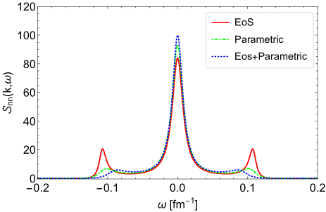
Figure 1: Variation of $\mathscr{S}_{nn}(\mathchoice{\mbox{\boldmath$k$}}{\mbox{\boldmath$k$}}{\mbox{\boldmath$\scriptstyle k$}}{\mbox{\boldmath$\scriptscriptstyle k$}},\omega)$ with $\omega$ for point ($r=0.2$) and $k=0.1$ fm^-1. Red line shows the effects of EoS with $\eta/s=\zeta/s=\kappa/s=1/4\pi$. The green line is obtained for parametric forms of thermodynamic quantities. And blue line is drawn with both effects.

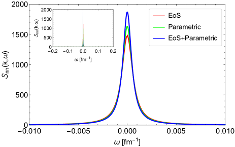
Figure 2: $\mathscr{S}_{nn}(\mathchoice{\mbox{\boldmath$k$}}{\mbox{\boldmath$k$}}{\mbox{\boldmath$\scriptstyle k$}}{\mbox{\boldmath$\scriptscriptstyle k$}},\omega)$ near the critical point for ($r=0.01$) and $k=0.1$ fm^-1. The red curve represents the effects of EoS and $\eta/s=\zeta/s=\kappa/s=1/4\pi$. The green line is obtained by using the scaling hypothesis of thermodynamic variables near CEP and both effects are shown in blue curve. Inset plot is for the broader range in $\omega$ ($-0.2\leq\omega\leq 0.2$).

Fig. 1 displays the variation of $\mathscr{S}_{nn}(\mathchoice{\mbox{\boldmath$k$}}{\mbox{\boldmath$k$}}{\mbox{\boldmath$\scriptstyle k$}}{\mbox{\boldmath$\scriptscriptstyle k$}},\omega)$ with $\omega$ when the system is away from CEP represented by $r=0.2$. Results with the effects of (i), (ii) as well as with the combined effects of (i)+(ii) are shown. To investigate the effects of EoS we keep the transport coefficients finite with values, $\eta/s,\zeta/s,\kappa/s=1/4\pi$. The relevant coupling and relaxation coefficients are estimated from Eq.18. We observe that for (i) there are three distinct peaks (red line). The central one is large and called the R-peak originates from the entropy fluctuation at constant pressure i.e. due to thermal fluctuation. The symmetric doublet about the R-peak are the B-peaks. The B-peaks originates from pressure fluctuation at constant entropy which is connected to sound wave. We find that the B-peaks are weaker than the R-peaks. (ii) We exclude the effects of EoS to investigate the effects of transport coefficients only near the CEP via their critical exponents in evaluating $\mathscr{S}_{nn}(\mathchoice{\mbox{\boldmath$k$}}{\mbox{\boldmath$k$}}{\mbox{\boldmath$\scriptstyle k$}}{\mbox{\boldmath$\scriptscriptstyle k$}},\omega)$. The dotted green curve in Fig. 1 depicts the $\mathscr{S}_{nn}(\mathchoice{\mbox{\boldmath$k$}}{\mbox{\boldmath$k$}}{\mbox{\boldmath$\scriptstyle k$}}{\mbox{\boldmath$\scriptscriptstyle k$}},\omega)$ obtained by using the scaling laws i.e when the parametric forms of the transport coefficients and response functions mentioned in Eq.35 are used. The B-peaks in scenario (ii) is sub-dominant, almost like a broad shoulder. The combined effects is depicted by the blue dotted line in Fig 1. It is observed that the combined effects make the B-peaks sub-dominant.

Closer to the CEP, however, the scenario changes drastically. The $\mathscr{S}_{nn}(\mathchoice{\mbox{\boldmath$k$}}{\mbox{\boldmath$k$}}{\mbox{\boldmath$\scriptstyle k$}}{\mbox{\boldmath$\scriptscriptstyle k$}},\omega)$ near the critical point ($r=0.01$) shows only the R-peak with height increased by more than an order of magnitude and the B-peaks vanish due to absorption of sound waves near CEP (Fig.2). The vanishing of B-peaks can be understood from the fact that in leading order the Brillouin frequencies, $\pm\omega_{B}\sim c_{s}k$ where $c_{s}$ is the velocity of sound. The effects of EoS is seen to reduce the height of the R-peak (red line).

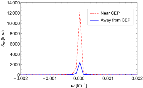
Figure 3: Variation of $\mathscr{S}_{nn}(\mathchoice{\mbox{\boldmath$k$}}{\mbox{\boldmath$k$}}{\mbox{\boldmath$\scriptstyle k$}}{\mbox{\boldmath$\scriptscriptstyle k$}},\omega)$ with $\omega$ for $r=0.01$ (red-line) and 0.2 (blue-line) corresponding to the situation of the system near and away from the CEP respectively. The value of $k$ is $0.02$ fm^-1 and $\eta/s=\zeta/s=\kappa/s=1/4\pi$.

The $\mathscr{S}_{nn}(\mathchoice{\mbox{\boldmath$k$}}{\mbox{\boldmath$k$}}{\mbox{\boldmath$\scriptstyle k$}}{\mbox{\boldmath$\scriptscriptstyle k$}},\omega)$ as a function of $\omega$ for smaller $k$ ($k=0.02$ fm^-1) is plotted in Fig.3 when only the effects of EoS is considered. The red (blue) line corresponds to results close to the CEP with $r=0.01$ (away from CEP with $r=0.2$, B-peaks are not visible because of the scale chosen along $\omega$ axis). We observe that at smaller $k$ the value of R-peak gets larger as well as sharper. A comparison with results shown in Fig.1 reveals that near CEP, the B-peaks vanish and the R-peak gets sharper and larger.

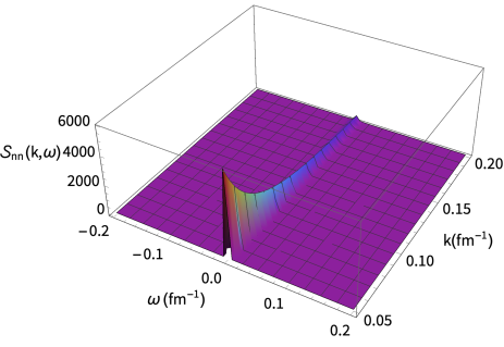
Figure 4: Variation of $\mathscr{S}_{nn}(\mathchoice{\mbox{\boldmath$k$}}{\mbox{\boldmath$k$}}{\mbox{\boldmath$\scriptstyle k$}}{\mbox{\boldmath$\scriptscriptstyle k$}},\omega)$ with $\omega$ and $k$ near the CEP ($r=0.01$) for $\eta/s=\zeta/s=\kappa/s=1/4\pi$

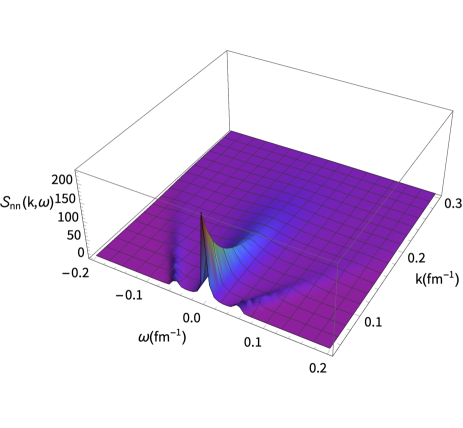
Figure 5: Same as Fig. 4 for $r=0.2$ i.e. the system is away from CEP.

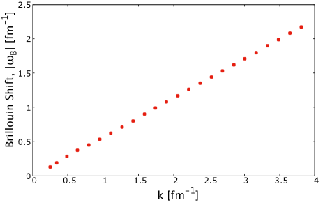
Figure 6: Variation of the Brillouin frequency, $\omega_{B}$ with $k$ when the system is away from CEP ($r=0.2$) with $\eta/s=\zeta/s=\kappa/s=1/4\pi$.

Motivated by the above results shown in Figs. 2 and 3 i.e. by observing the sensitivity of the results on the $k$ values we investigate the behaviour of spectral function for different hydrodynamic modes ($k-$modes). We consider the variation of $\mathscr{S}_{nn}(\mathchoice{\mbox{\boldmath$k$}}{\mbox{\boldmath$k$}}{\mbox{\boldmath$\scriptstyle k$}}{\mbox{\boldmath$\scriptscriptstyle k$}},\omega)$ with $k$ and $\omega$ near the CEP in Fig.4. We observe that for all values of $k$, the B-peaks merge with the R-peak. The height of the peak is maximum in the neighbourhood of $k\rightarrow 0$. In Fig.5 the $\mathscr{S}_{nn}(\mathchoice{\mbox{\boldmath$k$}}{\mbox{\boldmath$k$}}{\mbox{\boldmath$\scriptstyle k$}}{\mbox{\boldmath$\scriptscriptstyle k$}},\omega)$ is plotted against $\omega$ and $k$ when the system is away from CEP. We observe that the B-peaks shift away from R-peak with increase in $k$. This is better reflected in Fig.6, where the Brillouin frequency is plotted against $k$. A linear variation of $\omega$ with $k$ is obtained for given values of $T$ and $\mu$. The slope of the line is found to be 0.28 close to the velocity of sound $c_{s}=0.25$ obtained from Eq. 52 at the same value of temperature and chemical potential. Therefore, we find that the B-peaks move toward the R-peak as the system approach the CEP and ultimately merge with R-peak at the CEP. This suggests that the speed of propagation of all the hydrodynamic modes vanish at the CEP. This is consistent with the finding that the speed of sound reaches the minimum at QCD the critical point. The positions of the B-peak depends on $k$ when the system is away from CEP which indicates that the different k-modes travel with different speeds in the medium.

This nature of mode dependent speed of sound also signifies that the attenuation of the Mach-cone can not be interpreted as the unique effect of critical point as suggested in Ref. kunihiro . Rather mode dependent speed of propagation at points away from the CEP and vanishing speed of sound at CEP should be taken into account to properly interpret the attenuation of Mach-cone structure in the particle correlations.

VI summary and discussions

The correlation of density fluctuation near QCD critical point has been studied by using linearized perturbative equations obtained from Israel-Stewart hydrodynamics. The spectral structure, $\mathscr{S}_{nn}(\mathchoice{\mbox{\boldmath$k$}}{\mbox{\boldmath$k$}}{\mbox{\boldmath$\scriptstyle k$}}{\mbox{\boldmath$\scriptscriptstyle k$}},\omega)$ of the density fluctuation has been derived rigorously by keeping all the relevant transport coefficients and response functions non-zero. The effects of EoS and the critical behaviour of various transport coefficients on $\mathscr{S}_{nn}(\mathchoice{\mbox{\boldmath$k$}}{\mbox{\boldmath$k$}}{\mbox{\boldmath$\scriptstyle k$}}{\mbox{\boldmath$\scriptscriptstyle k$}},\omega)$ have been investigated.

The mode dependent propagation speed away from CEP suggests that careful look is needed for interpreting the suppression of Mach cone structure as a signature of CEP. These findings suggest that beam energy dependence of the correlation of number density fluctuation of produced particles in RHIC-E has the potential to carry the signature of critical point.

In condensed matter physics the effects of critical point have been investigated by measuring the intensity of the light scattered from the system. In contrast to this no such external probe is available for detecting CEP in QCD system. However, several possibilities for the detection of CEP in QCD have been discussed in the literature. In condensed matter system the phenomenon of critical opalescence at the CEP is considered as signal of large density fluctuations Stanley . The possibility of detecting the phenomenon of QCD opalescence by measuring the suppression of hadronic spectra in RHIC-E ($R_{AA}$) has been indicated in  csorgo . The $R_{AA}$ can be used to estimate the opacity factor, $\mathscr{K}$ as:

$$\mathscr{K}=-\frac{ln(R_{AA})}{R_{HBT}}$$ (36)

where $R_{HBT}$ is the Hanbury-Brown Twiss radius of the system.

The Fourier coefficients of the azimuthal distributions of particles can be used to understand various properties of the matter produced in RHIC-E. The coefficient of $cos3\phi$ (triangular flow) sheds light on the the initial fluctuations, similarly, the coefficients of $cos2\phi$ (elliptic flow) can be used to discern the EoS of the system. Near the critical point the order of the harmonics vary as $\sim 1/\lambda_{c}$ where $\lambda_{c}$ is the wavelength of the perturbation in pressure (sound) which diverges at the CEP and hence all the harmonics will vanish hasan . However, the experimentally measured spectra contains contribution from all the space-time points i.e. from all possible values of $T$ and $\mu$ not only from CEP. Therefore, even if the system passes through the CEP the Fourier coefficients may not vanish, but the CEP may depress them.

In Ref. Kapusta the mode-mode coupling theory has been used to study the existence and detection of CEP. It is comprehensively shown in  Kapusta that the thermal conductivity at CEP diverges which induces a sharp change in the two particle correlation of fluctuations in rapidity space. Detection of such modifications in the correlation function may confirm the existence of CEP. The suppression of fluctuations in temperature ($\Delta T$) and baryonic chemical potential ($\Delta\mu$) due to the divergence of thermodynamic response functions at CEP can signal the presence of CEP Stephanov:1998dy ; Stephanov:1999zu . The suppression in $\Delta T$ and $\Delta\mu$ will be reflected through the transverse momentum spectra of hadrons and proton to pion ratio respectively.

In reality, the possibility of the trajectories passing through the critical point is remote. This limits the fluctuations near CEP. These fluctuations will remain out of equilibrium due to critical slowing down stephanov3 . The creation of defects due to CEP in QCD like cosmology  kibble and condensed matter zurek systems and their detection will be extremely exciting. The appearance of Kibble-Zurek length scale and its connection with spatial correlations have been studied yakamatsu . The measurement of enhancement of non-flow correlations in presence of CEP as function of $n/s$ can be used to detect the CEP yakamatsu .

Rigorously speaking fluid dynamics works in the region where the condition, $k<<q$ is satisfied where $q$ is the inverse of correlation length which can be expresses as $q=q_{o}\,r^{\nu}$ $q_{o}$ is a constant and $\nu$ is the critical index with a numerical value $\nu=0.73\pm 0.02$ krg . This fundamental assumption becomes inoperative since $\xi$ diverges ($q\rightarrow 0$) at the CEP. However, there will be a region in the neighbourhood of CEP where the predictions of fluid dynamics may be useful. Following a procedure similar to condensed matter system Stanley we can write, $k<<q_{o}r^{\nu}$ for the validity of the hydrodynamics, which implies,

$$T>T_{c}\left[1+\left(\frac{k}{q_{o}}\right)^{1/\nu}\right]$$ (37)

Since hydrodynamics is an effective theory for soft physics (large wavelength or small wave vector, $k$), fluid dynamics can be applied in the neighbourhood of CEP but becomes invalid at CEP because of the divergence of the correlation length. The response of the trajectories in the neighbourhood of CEP in the $\mu-T$ plane to the initial conditions away from equilibrium has been investigated in Ref. tdore .

In a realistic scenario the matter formed in RHIC-E expands hydrodynamically which is not taken into consideration in the present work. The effects of the CEP in (3+1) dimensionally expanding system within the purview of second order viscous hydrodynamics is currently under investigation sksingh .

The physics of hadronic matter under extreme conditions of temperatures or densities and the QCD phase transition has been considered as the condensed matter physics of elementary particles cmp where the relevant microscopic interaction is controlled by non-abelian gauge theory in contrast to the condensed matter physics governed by abelian gauge theory. In condensed matter physics the theoretical results on dynamical spectral structure can be compared with the experimentally measured intensity of scattered of light. It has been shown that experimentally measured widths of R and B-peaks and one of the transport coefficients (among $\eta$, $\zeta$ and $\kappa$) as inputs will lead to the determination of the other two transport coefficients. Moreover, the integrated intensities of R and B-peaks has been connected to the Landau-Placzek ratio, $C_{p}/C_{v}-1=\gamma-1$. Identification of appropriate probes analogous to light in abelian system will go a long way to reveal the physics QCD matter near CEP.

VII Appendix A

In this appendix the expression for the dynamical spectral structure, $\mathscr{S}_{nn}(\mathchoice{\mbox{\boldmath$k$}}{\mbox{\boldmath$k$}}{\mbox{\boldmath$\scriptstyle k$}}{\mbox{\boldmath$\scriptscriptstyle k$}},\omega)$ derived by considering contributions up to second order in transport coefficients (i.e $\eta^{2},\zeta^{2},\kappa^{2},\eta\zeta,\eta\kappa,\zeta\kappa$) has been provided. The coupling and relaxation coefficients ($\alpha_{0},\alpha_{1},\beta_{0},\beta_{1},\beta_{2}$) have been taken non-zero in obtaining the results displayed in the text, but have been taken as zero in the following to avoid a more lengthy and complex expressions.

$$\mathscr{S^{\prime}}_{nn}(\mathchoice{\mbox{\boldmath$k$}}{\mbox{\boldmath$k$}}{\mbox{\boldmath$\scriptstyle k$}}{\mbox{\boldmath$\scriptscriptstyle k$}},\omega) = k^{2}n_{0}\Bigg{[}\omega^{2}n_{0}T^{2}\big{(}\frac{\text{$\partial$s}}{\text{$\partial$T}}\big{)}_{n}\Big{\{}h_{0}\kappa\omega+\big{(}\frac{\text{$\partial$p}}{\text{$\partial$T}}\big{)}_{n}k^{2}\big{(}\zeta+\frac{4}{3}\eta\big{)}-k^{2}T\kappa\omega^{2}+h_{0}k\kappa\big{(}\frac{\text{$\partial$s}}{\text{$\partial$n}}\big{)}_{T}$$ (38)

$$+k^{2}\kappa(\zeta+\frac{4}{3}\eta)-T^{2}\big{(}\frac{\text{$\partial$p}}{\text{$\partial$T}}\big{)}_{n}^{2}\Big{\}}+k^{2}\kappa h_{0}\Big{\{}-h_{0}T\big{(}\frac{\text{$\partial$p}}{\text{$\partial$T}}\big{)}_{n}+k^{2}\kappa(\zeta+\frac{4}{3}\eta)+T^{2}\big{(}\frac{\text{$\partial$p}}{\text{$\partial$T}}\big{)}_{n}^{2}\Big{\}}$$

$$+n_{0}^{2}T^{2}\big{(}\frac{\text{$\partial$s}}{\text{$\partial$T}}\big{)}_{n}\big{(}\frac{\text{$\partial$s}}{\text{$\partial$n}}\big{)}_{T}\Big{\{}\big{(}\frac{\text{$\partial$p}}{\text{$\partial$T}}\big{)}_{n}k(\zeta+\frac{4}{3}\eta)+T^{2}\kappa\omega^{2}-h_{0}\kappa\Big{\}}+k^{4}n_{0}h_{0}(\zeta+\frac{4}{3}\eta)^{2}$$

$$+h_{0}\big{(}\frac{\text{$\partial$p}}{\text{$\partial$n}}\big{)}_{T}\Big{\{}n_{0}T^{2}\omega^{2}\Big{(}k^{2}(\zeta+\frac{4}{3}\eta)+\kappa\omega^{2}-k^{2}\kappa\Big{)}\Big{\}}+h_{0}^{2}\kappa Tk^{2}\big{(}\frac{\text{$\partial$p}}{\text{$\partial$T}}\big{)}_{n}$$

$$-n_{0}h_{0}\kappa T^{2}k^{2}\omega^{2}\big{(}\frac{\text{$\partial$s}}{\text{$\partial$n}}\big{)}_{T}\Bigg{]}\Bigg{/}\Bigg{[}h_{0}^{2}\Big{\{}k^{4}\kappa^{2}\omega^{4}+n_{0}^{2}T^{2}\omega^{4}\big{(}\frac{\text{$\partial$s}}{\text{$\partial$T}}\big{)}_{n}\Big{\}}+h_{0}k^{2}\omega^{2}\kappa^{2}T^{2}\big{(}\frac{\text{$\partial$s}}{\text{$\partial$T}}\big{)}_{n}$$

$$\Big{\{}\omega^{4}-2n_{0}\big{(}\frac{\text{$\partial$p}}{\text{$\partial$n}}\big{)}_{T}\Big{\}}-2k^{2}n_{0}^{2}T^{2}\kappa^{2}\omega^{2}\big{(}\frac{\text{$\partial$s}}{\text{$\partial$T}}\big{)}_{n}^{2}-2n_{0}h_{0}k^{2}T^{2}\kappa^{2}\omega^{2}\big{(}\frac{\text{$\partial$p}}{\text{$\partial$T}}\big{)}_{n}$$

$$-2n_{0}^{3}T^{2}k^{4}\omega^{2}\big{(}\frac{\text{$\partial$s}}{\text{$\partial$T}}\big{)}_{n}\Big{\{}\big{(}\frac{\text{$\partial$p}}{\text{$\partial$T}}\big{)}_{n}\big{(}\frac{\text{$\partial$s}}{\text{$\partial$n}}\big{)}_{T}+\big{(}\frac{\text{$\partial$s}}{\text{$\partial$T}}\big{)}_{n}\big{(}\frac{\text{$\partial$p}}{\text{$\partial$n}}\big{)}_{T}\Big{\}}+k^{4}n_{0}^{4}T^{2}\omega^{2}\big{(}\frac{\text{$\partial$s}}{\text{$\partial$n}}\big{)}_{T}^{2}\big{(}\frac{\text{$\partial$p}}{\text{$\partial$n}}\big{)}_{T}^{2}$$

$$+2k^{2}n_{0}T\kappa\omega^{2}\big{(}\frac{\text{$\partial$p}}{\text{$\partial$T}}\big{)}_{n}\Big{\{}k^{4}\kappa\big{(}\frac{\text{$\partial$p}}{\text{$\partial$n}}\big{)}_{T}+T\omega^{2}\big{(}\frac{\text{$\partial$s}}{\text{$\partial$n}}\big{)}_{T}k^{2}(\zeta+\frac{4}{3}\eta)-T^{3}\kappa\omega^{2}\Big{\}}$$

$$+n_{0}^{2}T^{2}\Big{\{}h_{0}k^{2}\kappa^{2}\big{(}\frac{\text{$\partial$p}}{\text{$\partial$n}}\big{)}_{T}^{2}+k^{2}T^{2}\kappa^{2}\omega^{4}-2k^{4}T\kappa\omega^{4}\big{(}\frac{\text{$\partial$p}}{\text{$\partial$n}}\big{)}_{T}^{2}+2k^{2}h_{0}\kappa\omega^{2}(\zeta+\frac{4}{3}\eta)$$

$$+\big{(}\frac{\text{$\partial$s}}{\text{$\partial$T}}\big{)}_{n}^{2}k^{4}(\zeta+\frac{4}{3}\eta)^{2}+2k^{4}T\kappa\big{(}\frac{\text{$\partial$p}}{\text{$\partial$T}}\big{)}_{n}\big{(}\frac{\text{$\partial$s}}{\text{$\partial$n}}\big{)}_{T}(\zeta+\frac{4}{3}\eta)\Big{\}}\Bigg{]}\big{<}\delta n(\mathchoice{\mbox{\boldmath$k$}}{\mbox{\boldmath$k$}}{\mbox{\boldmath$\scriptstyle k$}}{\mbox{\boldmath$\scriptscriptstyle k$}},0)\delta n(\mathchoice{\mbox{\boldmath$k$}}{\mbox{\boldmath$k$}}{\mbox{\boldmath$\scriptstyle k$}}{\mbox{\boldmath$\scriptscriptstyle k$}},0)\big{>}$$

where

$$\mathscr{S}_{nn}(\mathchoice{\mbox{\boldmath$k$}}{\mbox{\boldmath$k$}}{\mbox{\boldmath$\scriptstyle k$}}{\mbox{\boldmath$\scriptscriptstyle k$}},\omega)=\frac{\mathscr{S^{\prime}}_{nn}(\mathchoice{\mbox{\boldmath$k$}}{\mbox{\boldmath$k$}}{\mbox{\boldmath$\scriptstyle k$}}{\mbox{\boldmath$\scriptscriptstyle k$}},\omega)}{\big{<}\delta n(\mathchoice{\mbox{\boldmath$k$}}{\mbox{\boldmath$k$}}{\mbox{\boldmath$\scriptstyle k$}}{\mbox{\boldmath$\scriptscriptstyle k$}},0)\delta n(\mathchoice{\mbox{\boldmath$k$}}{\mbox{\boldmath$k$}}{\mbox{\boldmath$\scriptstyle k$}}{\mbox{\boldmath$\scriptscriptstyle k$}},0)\big{>}}$$ (39)

The expression for $\mathscr{S}_{nn}(\mathchoice{\mbox{\boldmath$k$}}{\mbox{\boldmath$k$}}{\mbox{\boldmath$\scriptstyle k$}}{\mbox{\boldmath$\scriptscriptstyle k$}},\omega)$ contain derivatives of several thermodynamics quantities. In this appendix we recast these derivatives in terms of response functions like: isothermal and adiabatic compressibilities ($\kappa_{T}$ and $\kappa_{s}$), specific heats ($C_{p}$ and $C_{v}$), baryon number susceptibility ($\chi_{B}$) and velocity of sound ($c_{s}$), etc. The baryon number density ($n$) and the entropy density ($s$) can be written as:

$$n=\Big{(}\frac{\partial p}{\partial\mu}\Big{)}_{T};\,\,\,\,\,s=\Big{(}\frac{\partial p}{\partial T}\Big{)}_{\mu}$$ (40)

Baryon number susceptibility, isothermal compressibility and adiabatic compressibility are given by,

$$\chi_{B}=\Big{(}\frac{\partial n}{\partial\mu}\Big{)}_{T};\kappa_{T}=\frac{1}{n}\Big{(}\frac{\partial n}{\partial p}\Big{)}_{T};\kappa_{s}=\frac{1}{n}\Big{(}\frac{\partial n}{\partial p}\Big{)}_{s}$$ (41)

Specific heats can be expressed as:

$$C_{p}=T\Big{(}\frac{\partial s}{\partial T}\Big{)}_{p};C_{v} = T\Big{(}\frac{\partial s}{\partial T}\Big{)}_{V}=T\Big{(}\frac{\partial s}{\partial T}\Big{)}_{n}$$ (42)

$$= \Big{(}\frac{\partial\epsilon}{\partial T}\Big{)}_{V}=\Big{(}\frac{\partial\epsilon}{\partial T}\Big{)}_{n}$$

Now we write down the expression for partial derivatives, $(\frac{\partial p}{\partial T})_{n},(\frac{\partial p}{\partial n})_{T},(\frac{\partial\epsilon}{\partial T})_{n}$ and $\Big{(}\frac{\partial\epsilon}{\partial n}\Big{)}_{T}$ below. $(\frac{\partial p}{\partial T})_{n}$ can be evaluated as:

$$\Big{(}\frac{\partial p}{\partial T}\Big{)}_{n} = \frac{\partial(p,n)}{\partial(T,n)}$$ (43)

$$= \frac{\partial(p,n)}{\partial(T,p)}\frac{\partial(T,p)}{\partial(s,p)}\frac{\partial(s,p)}{\partial(s,\epsilon)}\frac{\partial(s,\epsilon)}{\partial(s,n)}\frac{\partial(s,n)}{\partial(T,n)}$$

$$= \Big{[}-\Big{(}\frac{\partial n}{\partial T}\Big{)}_{p}\Big{]}\Big{(}\frac{\partial T}{\partial s}\Big{)}_{p}\Big{(}\frac{\partial p}{\partial\epsilon}\Big{)}_{s}\Big{(}\frac{\partial\epsilon}{\partial n}\Big{)}_{s}\Big{(}\frac{\partial s}{\partial T}\Big{)}_{n}$$

$$= n\alpha_{p}\frac{T}{C_{p}}c^{2}_{s}\Big{(}\frac{\partial\epsilon}{\partial n}\Big{)}_{s}\frac{C_{v}}{T}$$

$$= nc^{2}_{s}\alpha_{p}\frac{C_{v}}{C_{p}}\Big{(}\frac{\partial\epsilon}{\partial n}\Big{)}_{s}$$

Using the relation,

$$d\epsilon=Tds+\mu dn\,\,\,\,\,\text{and }\mu=\Big{(}\frac{\partial\epsilon}{\partial n}\Big{)}_{s}$$ (44)

we write:

$$\Big{(}\frac{\partial p}{\partial T}\Big{)}_{n}=\mu nc^{2}_{s}\alpha_{p}\frac{C_{v}}{C_{p}}$$ (45)

Next we consider $\Big{(}\frac{\partial p}{\partial n}\Big{)}_{T}$:

$${\Big{(}\frac{\partial p}{\partial n}\Big{)}_{T}=\frac{1}{n\kappa_{T}}}$$ (46)

$$\Big{(}\frac{\partial p}{\partial n}\Big{)}_{T} = \frac{\partial(p,T)}{\partial(n,T)}=\frac{\partial(p,T)}{\partial(p,s)}\frac{\partial(p,s)}{\partial(\epsilon,s)}\frac{\partial(\epsilon,s)}{\partial(n,s)}\frac{\partial(n,s)}{\partial(n,T)}$$ (47)

$$= \Big{(}\frac{\partial T}{\partial s}\Big{)}_{p}\Big{(}\frac{\partial p}{\partial\epsilon}\Big{)}_{s}\Big{(}\frac{\partial\epsilon}{\partial n}\Big{)}_{s}\Big{(}\frac{\partial s}{\partial T}\Big{)}_{n}$$

$$= \frac{T}{C_{p}}c^{2}_{s}\Big{(}\frac{\partial\epsilon}{\partial n}\Big{)}_{s}\frac{C_{v}}{T}$$

$$= \mu c^{2}_{s}\frac{C_{v}}{C_{p}}$$ (48)

The factor, $\Big{(}\frac{\partial s}{\partial T}\Big{)}_{n}$ can be written as:

$$\Big{(}\frac{\partial s}{\partial T}\Big{)}_{n}=\frac{1}{T_{0}}\Big{(}\frac{T_{0}\partial s}{\partial T}\Big{)}_{n}=C_{v}$$ (49)

For fixed net baryon number, $c_{n}$ can be written as $c_{n}=C_{v}$. Therefore,

$${\Big{(}\frac{\partial\epsilon}{\partial T}\Big{)}_{n}=C_{v}}$$ (50)

We evaluate the derivative $\Big{(}\frac{\partial\epsilon}{\partial n}\Big{)}_{T}$ as

$$\Big{(}\frac{\partial s}{\partial n}\Big{)}_{T} = -\Big{(}\frac{\partial s}{\partial T}\Big{)}_{n}\Big{(}\frac{\partial T}{\partial n}\Big{)}_{s}=-\frac{1}{T_{0}}\Big{(}\frac{T\partial s}{\partial T}\Big{)}_{n}\Big{(}\frac{\partial T}{\partial n}\Big{)}_{s}$$ (51)

$$= -\frac{C_{v}}{T_{0}}\frac{1}{n_{0}}\Big{[}n_{0}\Big{(}\frac{\partial T}{\partial n}\Big{)}_{s}\Big{]}=\frac{C_{v}}{n_{0}T_{0}\alpha_{s}}$$

The velocity of sound is given by:

$$c_{s}^{2}=\Big{(}\frac{\partial p}{\partial\epsilon}\Big{)}_{s/n} = \frac{nd\mu+sdT}{\mu dn+Tds}$$ (52)

$$= \frac{nFdT+sdT}{\mu(\frac{\partial n}{\partial T})_{\mu}dT+\mu(\frac{\partial n}{\partial\mu})_{T}d\mu+T(\frac{\partial s}{\partial T})_{\mu}dT+T(\frac{\partial s}{\partial\mu})_{T}d\mu}$$

$$= \frac{nFdT+sdT}{\mu(\frac{\partial n}{\partial T})_{\mu}dT+\mu F(\frac{\partial n}{\partial\mu})_{T}dT+T(\frac{\partial s}{\partial T})_{\mu}dT+TF(\frac{\partial s}{\partial\mu})_{T}dT}$$

$$= \frac{nF+s}{\mu(\frac{\partial n}{\partial T})_{\mu}+\mu F(\frac{\partial n}{\partial\mu})_{T}+T(\frac{\partial s}{\partial T})_{\mu}+TF(\frac{\partial s}{\partial\mu})_{T}}$$

where,

$$F = \frac{(\frac{\partial s}{\partial T})_{\mu}-\frac{s}{n}(\frac{\partial n}{\partial T})_{\mu}}{\frac{s}{n}(\frac{\partial n}{\partial\mu})_{T}-(\frac{\partial s}{\partial\mu})_{T}}$$

VIII Acknowledgement

M.R. is supported by Department of Atomic Energy (DAE), Govt. of India. The work of AB is supported by Alexander von Humboldt (AvH) foundation and Federal Ministry of Education and Research (Germany) through Research Group Linkage programme. AB also thanks Purnendu Chakraborty, Sourin Mukhopadhyay and Soumen Datta for fruitful discussions.

References

- (1) N. Cabibbo and G. Parisi, Phys. Lett. B 59, 67 (1975).
- (2) J. C. Collins and M. Perry,Phys. Rev. Lett. 34, 1353 (1975).
- (3) K. Yagi, T. Hatsuda, and Y. Miake, Quark Gluon Plasma, Cambridge University Press (2005).
- (4) C.Y. Wong, Introduction to high-energy heavy ion collisions, World Scientific (1994).
- (5) W. Busza, K. Rajagopal and W. van der Schee,Ann. Rev. Nucl. Part. Sci. 68, 339 (2018), [arXiv:1802.04801 [hep-ph]].
- (6) E. V. Shuryak,Phys. Rept. 61, 71-158 (1980).
- (7) BRAHMS Collaboration: I Arsene et al, Nucl. Phys. A 757, 1 (2005); PHOBOS Collaboration: B B Back et al, Nucl. Phys. A 757, 28 (2005); STAR Collaboration: J Adams et al, Nucl. Phys. A 757, 102 (2005); PHENIX Collaboration: K Adcox et al, Nucl. Phys. A 757, 184 (2005).
- (8) Z. Fodor and S. Katz,JHEP 03, 014 (2002), [arXiv:hep-lat/0106002 [hep-lat]].
- (9) M. Asakawa and K. Yazaki,Nucl. Phys. A 504, 668 (1989).
- (10) A. M. Halasz, A. Jackson, R. Shrock, M. A. Stephanov and J. Verbaarschot, Phys. Rev. D 58, 096007 (1998), [arXiv:hep-ph/9804290 [hep-ph]].
- (11) P. de Forcrand and O. Philipsen,Nucl. Phys. B 642, 290 (2002), [arXiv:hep-lat/0205016 [hep-lat]].
- (12) Y. Aoki, G. Endrodi, Z. Fodor, S. Katz and K. Szabo,Nature 443, 675 (2006), [arXiv:hep-lat/0611014 [hep-lat]].
- (13) G. Endrodi, Z. Fodor, S. Katz and K. Szabo,JHEP 04, 001 (2011), [arXiv:1102.1356 [hep-lat]].
- (14) Z. Fodor and S. Katz,JHEP 04, 050 (2004), [arXiv:hep-lat/0402006 [hep-lat]].
- (15) R. V. Gavai,Pramana 84, no.5, 757 (2015), [arXiv:1404.6615 [hep-ph]].
- (16) A. Bhattacharyya, P. Deb, S. K. Ghosh and R. Ray, Phys. Rev. D 82 014021 (2010).
- (17) A. Bhattacharyya, P. Deb, A. Lahiri and R. Ray, Phys. Rev. D 82 114028 (2010).
- (18) A. Bhattacharyya, P. Deb, A. Lahiri and R. Ray, Phys. Rev. D 83 014011 (2011).
- (19) B. J. Schaefer, J. M. Pawlowski and J. Wambach, Phys. Rev. D 76 074023 (2007).
- (20) T. K. Herbst, J. M. Pawlowski and B. J. Schaefer, Phys. Lett. B 696 58 (2011).
- (21) J. Wambach, B. J. Schaefer and M. Wagner, Acta Phys. Polon. Supp. 3 691 (2010).
- (22) M. Aggarwal et al. [STAR], [arXiv:1007.2613 [nucl-ex]].
- (23) H. E. Stanley, Introduction to phase transitions and critical phenomena, Oxford University Press, 1971.
- (24) Y. Minami and T. Kunihiro, Prog. Th. Phys. 122, 881 (2009).
- (25) W. Assawasunthonnet; https://dspace.mit.edu/handle/1721.1/51611.
- (26) C. Nonaka, M. Asakawa, Phys. Rev. C 71 044904 (2005).
- (27) M. Hasanujjaman, M. Rahaman, A. Bhattacharyya, J. Alam, arXiv:2003.07575[nucl-th].
- (28) L.M. Satarov, M.N. Dmitriev, and I.N. Mishustin. arXiv:0901.1430v1.
- (29) A. Andronic, P. Braun-Munzinger, J. Stachel, and M. Winn, Phys. Lett. B 718, 80 (2012).
- (30) G. Sarwar, S. Chatterjee and J. Alam, J. Phys. G 44, 055101 (2017).
- (31) W. Israel and J. M. Stewart, Ann. Phys. 118, 341 (1979).
- (32) I. Muller, Z. Phys. 198, 329 (1967).
- (33) L. D. Landau and E. M. Lifshitz, Fluid Mechanics (AddisonWesley, Boston, 1959).
- (34) C. Eckart, Phys. Rev. 58, 919 (1940).
- (35) W. A. Hiscock, L. Lindblom, Ann. of Phys., 151 466 (1983).
- (36) P. Van, P. S. Biro, Eur, Phys. Jour. Special Topics, 155, 201(2008).
- (37) R. Baier, P. Romatschke, D. T. Son, A. O. Starinets and M. A. Stephanov, J. High Energ. Phys 04 100 (2008).
- (38) A. Muronga, Phys. Rev. C 76, 014909 (2007).
- (39) P. Romatchske, Int. J. of Mod. Phys. E 19, 1 (2010).
- (40) S. Lahiri, arXiv:1908.09462, Class. Quantum Grav. 37, 075010 (2020).
- (41) S. Grozdanov, P. K. Kovtun, A. O. Starinets, et. al. J. High Energ. Phys. 97 2019, (2019).
- (42) T. Csörgö, PoS CPOD2009 (2009) 035, [0911.5015 [nucl-th].
- (43) J. I. Kapusta and J. M. Torres-Rincon, Phys. Rev. C 86, 054911 (2012)
- (44) R. Guida and J. Zinn-Justin, Nuclear Physics B 489, 626 (1997).
- (45) M. A. Stephanov, K. Rajagopal and E. V. Shuryak,Phys. Rev. Lett. 81, 4816 (1998), [arXiv:hep-ph/9806219 [hep-ph]].
- (46) M. A. Stephanov, K. Rajagopal and E. V. Shuryak,Phys. Rev. D 60, 114028 (1999), [arXiv:hep-ph/9903292 [hep-ph]].
- (47) M. Stephanov, and Y. Yin, Phys. Rev. D 98, 036006(2018).
- (48) T. W. B. Kibble, Phys. Rep. 67, 183 (1980).
- (49) W. H. Zurek, Nature. 317, 505 (1985).
- (50) Y. Akamatsu, D. Teaney, F. Yan, and Yi. Yin, Phys. Rev. C, 100 044901 (2019).
- (51) K. Rajagopal and F. Wilczek, Nucl. Phys. B 399, 395 (1993).
- (52) T. Dore, J. Noronha-Hostler and E. McLaughlin, arXiv 2007.15083 [nucl-th].
- (53) S. K. Singh, work under progress.
- (54) K. Rajagopal and F. Wilczek, arXiv:hep-ph/0011333; https://doi.org