Supernova-scope for the Direct Search of Supernova Axions

Shao-Feng Ge^a,b,c, Koichi Hamaguchi^d,e, Koichi Ichimura^f,e Koji Ishidoshiro^f, Yoshiki Kanazawa^d, Yasuhiro Kishimoto^f,e, Natsumi Nagata^d, Jiaming Zheng^a,b

^aTsung-Dao Lee Institute, Shanghai 200240, Shanghai Jiao Tong University, China
^bSchool of Physics and Astronomy, Shanghai Jiao Tong University, Shanghai 200240, China
^cShanghai Key Laboratory for Particle Physics and Cosmology, Shanghai Jiao Tong University, Shanghai 200240, China
^dDepartment of Physics, University of Tokyo, Bunkyo-ku, Tokyo 113–0033, Japan

^eKavli IPMU (WPI), University of Tokyo, Kashiwa, Chiba 277–8583, Japan

^fResearch Center for Neutrino Science, Tohoku University, Sendai 980–8578, Japan

If a supernova explosion occurs within a few hundred parsecs from the Earth, a huge number of axions, in addition to neutrinos, may arrive at the Earth. In this paper, we discuss in detail the prospect of detecting those supernova axions by an axion helioscope. With the help of a pre-supernova neutrino alert system, it is possible to point a helioscope at an exploding supernova in advance. The supernova axions can then be detected by a gamma-ray detector installed at the end of the helioscope. We call such a detection system an axion supernova-scope (SNscope). We propose a conceptual design for an axion SNscope, where the gamma-ray detector is installed at the opposite end to the X-ray detector for the solar axion. It still functions as an axion helioscope during the normal operation time, and once a pre-SN neutrino alert is received, the scope is temporarily turned around and targeted to a SN candidate, waiting for the supernova axions. We estimate the sensitivity of supernova axion detection and find that SNscopes based on the next-generation axion helioscopes, such as IAXO, have potential to explore the invisible axions and to test the axion interpretation of stellar cooling anomalies.

1 Introduction

Axion [1, 2] is a pseudo Nambu-Goldstone boson associated with the spontaneous breaking of the Peccei-Quinn symmetry [3, 4], which was introduced to solve the strong CP problem. Although the original axion model has already been excluded by experiment, its simple extensions—called invisible axion models [5, 6, 7, 8]—are perfectly viable and capable of solving the strong CP problem. The characteristic features of the invisible axions are tiny mass and extremely weak couplings to the Standard Model particles. The latter property helps the invisible axions to evade the experimental constraints with the price of making it very challenging to test these models.

Stellar objects offer promising ways of testing axions and provide stringent constraints on axion models. For instance, the observed duration of the neutrino signal from SN1987A [9, 10, 11] provides one of the strongest bounds on axions [12, 13, 14, 15, 16, 17, 18, 19, 20]. The temperature observations of certain neutron stars also give severe limits on axion models [22, 23, 24], which are as strong as the SN1987A bound. On the other hand, several observations indicate some preference for the presence of extra stellar energy losses, which may be attributed to axion [25, 26, 27, 28].

These astrophysical limits/hints are in general given by indirect searches of axions and suffer from considerable uncertainty from both theory and observation. It would be of great advantages to have direct searches for astrophysical axions. The axion helioscopes [29] designed for detecting solar axions are suitable and promising tools for this purpose. Several axion helioscope experiments have been performed so far and imposed limits on the axion-photon coupling [30, 31, 32, 33, 34, 35, 36, 37, 38, 39]. Next-generation helioscopes, such as the International Axion Observatory (IAXO) [40, 41] and Trioitsk Axion Solar Telescope Experiment (TASTE) [42], are being planned and expected to have significantly improved sensitivities.

Axion helioscopes can be pointed at not only the Sun but also other celestial objects. An interesting possibility of such an application is to detect a burst of axions from a nearby supernova (SN) explosion. It is in principle possible to target helioscopes at an exploding SN in advance with the help of a pre-SN neutrino alert system, such as the Supernova Early Warning System (SNEWS) [43]. The SN axions then convert to photons inside the helioscope, which can be detected if a $\gamma$-ray detector is installed on the end of the helioscope. Indeed, there have been brief speculations on such a possibility in the literature [25, 44]. In this paper, we study in detail the prospect of detecting SN axions with an operating helioscope and propose a conceptual design for the detection setup, which we call the axion supernova-scope (SNscope). The gamma-ray detector is installed at the opposite end to the X-ray detector for the solar axion. The experiment can work as an axion helioscope during the normal operation time, and once a pre-SN neutrino alert is received, the scope is turned around and targeted at a SN candidate, waiting for the SN axions. We show that the axion SNscopes based on the next-generation axion helioscopes can probe invisible axions if a SN explosion occurs within a few hundred parsecs from the Earth. The SN axion detection is a realistic and promising option for extending the physics potential of the future axion helioscopes.

The outline of this paper is the following. In Sec. 2, we review relevant features of invisible axions and the present constraints on them. In Sec. 3, we list nearby SN progenitor candidates and discuss the pre-SN neutrino alert system that may forecast SN explosions. In Sec. 4, we show the layout of axion SNscopes which we discuss in this paper. We then evaluate the observational probability for each SN progenitor candidate, estimate the number of SN axion events detected by an axion SNscope, and discuss the background for this in Sec. 5. Section 6 summarizes our conclusions.

2 Axion

Axion [1, 2] is a pseudo Nambu-Goldstone boson which appears below the symmetry-breaking scale of the global U(1) Peccei-Quinn symmetry [3, 4]. This energy scale is characterized by the axion decay constant $f_{a}$. For the invisible axion, such as the KSVZ [5, 6] and DFSZ [7, 8] models, $f_{a}$ is much larger than the electroweak scale and the interactions of the axion at low energies are described by the following effective Lagrangian,

$${\cal L}_{\rm int} =\frac{\alpha_{s}}{8\pi}\frac{a}{f_{a}}G^{a\mu\nu}\widetilde{G}^{a}_{\mu\nu}+\frac{g_{a\gamma\gamma}}{4}aF_{\mu\nu}\widetilde{F}^{\mu\nu}+\sum_{f}\frac{C_{f}}{2f_{a}}\bar{f}\gamma^{\mu}\gamma_{5}f\partial_{\mu}a+\dots~{},$$ (1)

where $a$ is the axion field, $\alpha_{s}\equiv g_{s}^{2}/(4\pi)$ with $g_{s}$ being the strong gauge coupling constant, $G^{a}_{\mu\nu}$ and $F_{\mu\nu}$ are the field strength tensors of the color and electromagnetic gauge fields, respectively, $\widetilde{G}^{a}_{\mu\nu}\equiv\frac{1}{2}\epsilon_{\mu\nu\rho\sigma}G^{a\rho\sigma}$ and $\widetilde{F}_{\mu\nu}\equiv\frac{1}{2}\epsilon_{\mu\nu\rho\sigma}F^{\rho\sigma}$ with $\epsilon^{\mu\nu\rho\sigma}$ the totally antisymmetric tensor, $f$ denotes the Standard Model fermions, and the dots indicate higher-dimensional operators which are irrelevant to our discussions.

At the leading order in chiral perturbation theory with two quark flavors, the axion mass $m_{a}$ is [1]

$$m_{a}=\frac{\sqrt{m_{u}m_{d}}}{m_{u}+m_{d}}\frac{f_{\pi}m_{\pi}}{f_{a}}\simeq 5.8\times\biggl{(}\frac{f_{a}}{10^{9}~{}\mathrm{GeV}}\biggr{)}^{-1}~{}\mathrm{meV}~{},$$ (2)

where $m_{u}=2.16$ MeV, $m_{d}=4.67$ MeV, $m_{\pi}=135$ MeV are the masses of up quark, down quark, and the neutral pion, respectively, and $f_{\pi}=92.1$ MeV [45] is the pion decay constant. The next-to-next-to-leading order computation in chiral perturbation theory and a recent calculation with QCD lattice simulations of $m_{a}$ can be found in [48] and [49], respectively, whose results are consistent with Eq. (2) up to ${\cal O}(1-10)\%$ corrections.

The coupling of the axion-photon interaction, $g_{a\gamma\gamma}$, is a model-dependent parameter. Its value is inversely proportional to $f_{a}$ and is given by, at the leading order in chiral perturbation theory,

$$g_{a\gamma\gamma}=\frac{\alpha}{2\pi f_{a}}\biggl{[}\frac{E}{N}-\frac{2}{3}\frac{4m_{d}+m_{u}}{m_{u}+m_{d}}\biggr{]}\simeq\frac{\alpha}{2\pi f_{a}}\biggl{[}\frac{E}{N}-2.0\biggr{]}~{},$$ (3)

where $\alpha$ is the fine-structure constant, and $E/N$ is the ratio between the electromagnetic and color anomaly factors for the Peccei-Quinn current; for instance, $E/N=8/3$ in the DFSZ model while $E/N=0$ in the KSVZ model with electrically neutral Peccei-Quinn fermions. The next-to-leading order calculation of $g_{a\gamma\gamma}$ in chiral perturbation theory is available in [50], which is in good agreement with Eq. (3). This axion-photon coupling determines the axion-to-photon conversion rate in a helioscope/SNscope.

At low energies, the axion-gluon (the first term) and axion-quark (the third term) interactions in Eq. (1) induce the axion-nucleon couplings, which have the form

$${\cal L}_{aNN}=\sum_{N=p,n}\frac{C_{N}}{2f_{a}}\bar{N}\gamma^{\mu}\gamma_{5}N\partial_{\mu}a\equiv\sum_{N=p,n}\frac{g_{aN}}{2m_{N}}\bar{N}\gamma^{\mu}\gamma_{5}N\partial_{\mu}a,$$ (4)

where $g_{aN}\equiv C_{N}m_{N}/f_{a}$. At the leading order in $\alpha_{s}$, the coefficients $C_{N}$ are given by

$$C_{N}=\sum_{q}\biggl{(}C_{q}-\frac{m_{*}}{m_{q}}\biggr{)}\Delta q^{(N)}~{},$$ (5)

where $m_{*}\equiv m_{u}m_{d}m_{s}/(m_{u}m_{d}+m_{d}m_{s}+m_{u}m_{s})$ with $m_{s}$ being the strange quark mass. The factor $\Delta q^{(N)}$ is the spin fraction defined by $2s_{\mu}^{(N)}\Delta q^{(N)}\equiv\langle N|\bar{q}\gamma_{\mu}\gamma_{5}q|N\rangle$ with $s_{\mu}^{(N)}$ denoting the spin of the nucleon $N$: $\Delta u^{(p)}=\Delta d^{(n)}=0.897(27)$, $\Delta d^{(p)}=\Delta u^{(n)}=-0.376(27)$, and $\Delta s^{(p)}=\Delta s^{(n)}=-0.026(4)$ [50]. The QCD corrections to Eq. (5) are considered in [50]. For the KSVZ axion ($C_{q}=0$), we have [50]

$$C_{p}=-0.47(3)~{},\qquad C_{n}=-0.02(3)~{},$$ (6)

and for the DFSZ axion ($C_{u,c,t}=\cos^{2}\beta/3$ and $C_{d,s,b}=\sin^{2}\beta/3$ with $\tan\beta$ denoting the ratio of the vacuum expectation values of the two doublet Higgs fields, $\tan\beta\equiv\langle H_{u}\rangle/\langle H_{d}\rangle$) [45],

$$C_{p} =-0.182(25)-0.435\sin^{2}\beta~{},$$ (7a)

$$C_{n} =-0.160(25)+0.414\sin^{2}\beta~{}.$$ (7b)

These axion-nucleon couplings determine the production rate of axions in SN explosions.

Let us now discuss the limits on the axion couplings from stellar cooling. One of the strongest constraints is derived from the measured neutrino signal duration of SN1987A [12, 13, 14, 15, 16, 17, 18, 19, 20]. In a recent analysis [20], the constraint on the axion-nucleon couplings is obtained as $g_{an}^{2}+0.61g_{ap}^{2}+0.53g_{an}g_{ap}\lesssim 8.26\times 10^{-19}$, by imposing the condition that the axion luminosity ($L_{a}$) at the post-bounce time $t_{\rm pb}=1$ sec should not exceed the neutrino luminosity ($L_{\nu}$), $L_{a}\lesssim L_{\nu}\simeq 2\times 10^{52}\,{\rm erg}\;{\rm s}^{-1}$. This corresponds to $f_{a}\gtrsim 3.9\times 10^{8}$ GeV for KSVZ and $f_{a}\gtrsim 4.7\times 10^{8}$ GeV for DFSZ with $\tan\beta=10$. We note that these constraints should be considered as indicators rather than sharp bounds with the present limited understanding of the SNe [45]. It was also pointed out recently [21] that the observed neutrinos from SN1987A might have come from an accretion disk that would not be cooled by emitting axions. If this is the case, the criteria $L_{a}\lesssim L_{\nu}$ is not applicable and neither are the bounds obtained with it.

Another stringent constraint on the axions is given by the temperature observations of neutron stars [22, 23, 24]. The cooling of the neutron star in the SN remnant Cassiopeia A (Cas A) is studied in Ref. [22], which gives $f_{a}\gtrsim\sqrt{0.9C_{p}^{2}+1.4C_{n}^{2}}\times 10^{9}$ GeV; this leads to $f_{a}\gtrsim 5\times 10^{8}$ GeV for KSVZ and $f_{a}\gtrsim 7\times 10^{8}$ GeV for DFSZ with $\tan\beta=10$. Another hot young neutron star in the SN remnant HESS J1731-347 requires $f_{a}\gtrsim 3.4|C_{n}|\times 10^{9}$ GeV [23], which gives $f_{a}\gtrsim 7\times 10^{7}$ GeV for KSVZ and $f_{a}\gtrsim 8\times 10^{8}$ GeV for DFSZ with $\tan\beta=10$. We stress again that there can be ${\cal O}(1)$ uncertainty in these bounds (see, e.g., the discussion on the uncertainty coming from the envelope composition of the Cas A neutron star in [22]). For the other stellar cooling constraints on the axion couplings, see [45] and references therein, and also [51].

Finally, it has been pointed out that several observations of other astrophysical objects, such as white dwarfs, red giant branch stars, and horizontal branch stars, may point to the existence of additional source of stellar cooling beyond the standard cooling sources, and it may be the hint of the axion [25, 26, 27, 28]. This cooling hint prefers a value of $f_{a}$ lower than the limits quoted above; for example, in [27], the best fit value for $f_{a}$ is obtained for the DFSZ model as $f_{a}=7.7\times 10^{7}$ GeV and $\tan\beta=0.28$ if the SN1987A constraint is not included. These cooling hints also suffer from large uncertainty in both theory and observation.

Given the significance of these astrophysical limits/hints on axions as well as their large uncertainty, it is desirable to consider a more direct way of probing axions produced from the stellar objects mentioned above. Among them, SNe are the most promising target because of the prominent luminosity of axions emitted during the first ten seconds from the explosion. In what follows, we discuss a strategy for the detection of SN axions by adapting an axion helioscope.

3 Nearby SN candidates and pre-SN neutrino alarm

Even before a core-collapse SN explosion, a large number of neutrinos are emitted from the progenitor [56]. These pre-SN neutrinos are produced during the last stages of the stellar evolution and typically have energies of 1–2 MeV. The calculation of the flux of pre-SN neutrinos has been performed in the literature [56, 57, 58, 59, 60, 61, 62, 63, 64, 65, 66], showing that it is possible to detect them if the progenitor star is located sufficiently near the Earth ($\lesssim 1$ kpc). In particular, the on-going/future neutrino experiments, e.g., KamLAND [67], SNO+ [68], Super-Kamiokande [69], Hyper-Kamiokande [70], JUNO [71], and DUNE [72, 73], as well as future dark matter detectors [74], are expected to be sensitive to pre-SN neutrinos, which provide a possibility of forecasting the occurrence of a SN event in advance [56]. This global network of these experiments developed for an early SN alarm is called SNEWS [43, 75, 76].

Table 1: List of SN progenitor candidates with having a mass $\gtrsim 10~{}M_{\odot}$ and within $250$ pc from the Earth. We basically use the values listed in the Hipparcos catalogue [78]; otherwise, we show the reference for the source.

HIP	Common Name	Distance (pc)	Mass ($M_{\odot}$)	RA (J2000)	Dec (J2000)
65474	Spica/$\alpha$ Virginis	77(4)	$11.43\pm 1.15$ [79]	13:25:11.58	$-11$:09:40.8
81377	$\zeta$ Ophiuchi	112(3)	$20.0$ [80]	16:37:09.54	$-10$:34:01.5
71860	$\alpha$ Lupi	142(3)	$10.1\pm 1.0$ [81]	14:41:55.76	$-47$:23:17.5
80763	Antares/$\alpha$ Scorpii	170(30)	11–14.3 [82]	16:29:24.46	$-26$:25:55.2
107315	Enif/$\epsilon$ Pegasi	211(8)	11.7(8) [81]	21:44:11.16	$+09$:52:30.0
27989	Betelgeuse/$\alpha$ Orionis	$222^{+48}_{-34}$ [83]	$11.6^{+5.0}_{-3.9}$ [84]	05:55:10.31	$+07$:24:25.4

As we discuss in Sec. 5, SN axions may be detectable if the SN is within a few hundred parsecs from the Earth. For such a nearby SN, it is quite likely that the SNEWS gives an alert prior to the SN explosion. There are a sizable number of stars within this range that are considered to be exploding in the near future; we summarize the progenitor candidates of core-collapse SNe within the distance $d\leq 250$ pc from the Earth in Table 1, which we have taken from Refs. [85, 86, 87]. In this table, we show both red and blue (super)giant stars that have a mass $M\gtrsim 10~{}M_{\odot}$, for which an iron core is expected to be formed prior to the stellar collapse. For a more complete list of nearby SN progenitor candidates, see, e.g., Table A1 of Ref. [87]. In Table 1, the first column shows the Hipparcos Catalogue number, and the fifth and sixth columns are J2000 right ascension and declination, respectively. We also show the distribution of these stars on the Mollweide projection of the celestial sphere in Fig. 1, where the red and blue dots correspond to the spectral types of K/M and O/B, respectively. We also show by the gray dots the progenitors with $d>250$ pc and $M\gtrsim 10~{}M_{\odot}$ listed in Table A1 of Ref. [87].

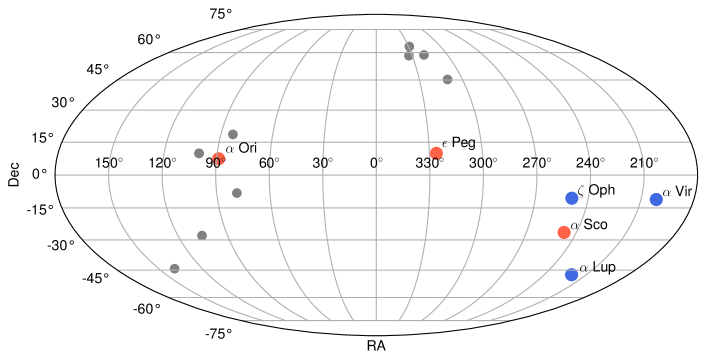
Figure 1: The position of the SN progenitors in Table 1 on the Mollweide projection of the celestial sphere, where the red and blue dots correspond to the spectral types of K/M and O/B, respectively. We also show by the gray dots the progenitors with $d>250$ pc and $M\gtrsim 10~{}M_{\odot}$ listed in Table A1 in Ref. [87].

With pre-SN neutrinos, it is in principle possible to estimate the location of the source on the sky, which would be useful to identify the progenitor [91, 87]. A liquid scintillator detector, such as JUNO [71], can use the inverse beta decay process, $\bar{\nu}_{e}+p\to n+e^{+}$, to reconstruct the direction of the incoming anti-neutrino. The angular resolution obtained with a JUNO-like detector at ${\cal O}(1)$ hours before the SN explosion is estimated to be $\simeq 60^{\circ}$ [87] for a nearby progenitor as in Table 1. This information by itself can narrow the list of candidates down to a few. Moreover, if a detector with a better angular sensitivity is available in the future, the precision of the progenitor identification is considerably improved. For instance, a lithium-loaded liquid scintillator [92] may be able to give an angular resolution of $\simeq 15^{\circ}$ [87], with which we can most likely identify the progenitor star uniquely. All in all, it is feasible to determine the exploding nearby progenitor with a pre-SN neutrino alert system by ${\cal O}(1)$ hours before the explosion, which thus makes it possible to direct an axion SNscope at the progenitor in advance.

4 Axion SNscope

An axion helioscope [29] is a tool to detect the axion flux from the Sun, in which an incoming axion is converted into a photon while it passes through the strong magnetic field inside the helioscope. The converted photon is then detected by a X-ray detector placed on its end side. Previous axion helioscope experiments have not yet detected axion signatures, imposing constraints on axion models [30, 31, 32, 33, 34, 35, 36, 37, 38, 39]. Among these experiments, the CERN Axion Solar Telescope (CAST) experiment gives the most stringent limit on the axion-photon coupling: $g_{a\gamma\gamma}<0.66\times 10^{-10}~{}{\rm GeV}^{-1}$ for $m_{a}<0.02$ eV [39].

Table 2: List of the on-going and next-generation helioscopes as well as their (proposed) site, magnetic field strength $B$, length $L$, and cross sectional area $A$.

Experiment	(Proposed) site	$B$ (T)	$L$ (m)	$A$ (m2)
CAST [34, 35, 36, 37, 38, 39]	CERN	9	9.3	$2.9\times 10^{-3}$
BabyIAXO [41]	DESY	$\sim 2$	10	$0.77$
IAXO baseline [40, 41]	DESY	$\sim 2.5$	$20$	$2.3$
IAXO+ [41]	DESY	$\sim 3.5$	$22$	$3.9$
TASTE [42]	INR	3.5	12	0.28

There are several proposals for next-generation helioscopes, which we summarize with their properties in Table 2. IAXO [40, 41] was proposed as a follow-up of CAST and is planned to be built at DESY. It consists of eight bores of 600 mm diameter and a 25 m long toroidal superconducting magnet, which provides $\sim 2.5$ T magnetic field in the bores on average. This setup, called the IAXO baseline, realizes a total cross section area of $2.3$ m². Prior to IAXO, an experiment with a prototype helioscope with two 10 m long bores, called BabyIAXO [41], is going to be performed. This prototype experiment offers not only physics outcome with a sensitivity better than that of CAST but also opportunities to test potential improvements in the technical design. With this feedback, we may have an improved version of IAXO in the future, which we refer to as the IAXO+ [41] in Table 2. Meanwhile, another axion helioscope called TASTE [42] is projected to be constructed in the Institute for Nuclear Research (INR) in Russia. We show the relevant parameters of these axion helioscopes—the magnetic field strength $B$, length $L$, and cross sectional area $A$—in Table 2.

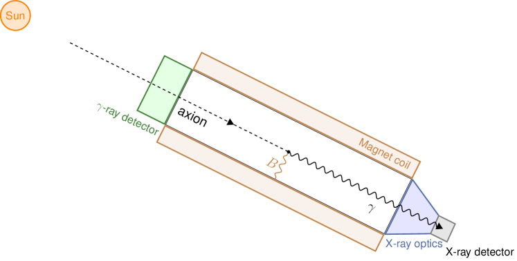
(a) Axion helioscope

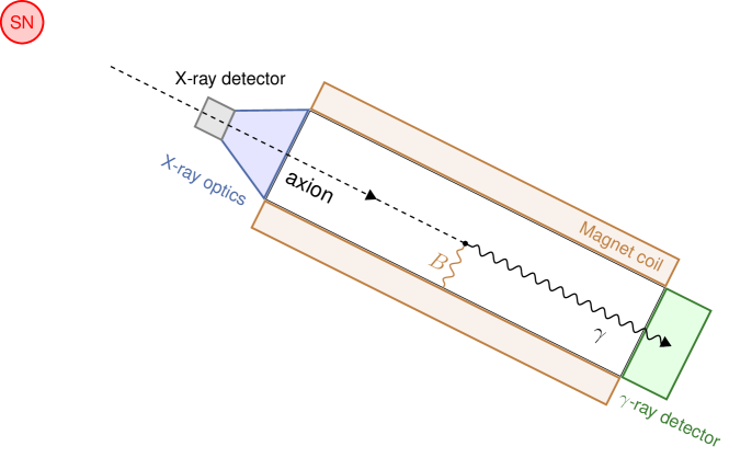
(b) Axion SNscope

Figure 2: Conceptual design of the axion detector discussed in this paper and its orientation for the detection of (a) solar and (b) SN axions.

With the help of the pre-SN neutrino alarm discussed in the previous section, we can direct an axion helioscope at an exploding progenitor in advance, aiming at the detection of SN axions. Nevertheless, it is not possible to merely use an axion helioscope as it is for this purpose, since SN axions typically have energies of ${\cal O}$(10–100) MeV as we will show in Sec. 5.2 and thus the converted photons have a wavelength in the $\gamma$-ray range. This requires an additional installation of a $\gamma$-ray detector on a helioscope. For instance, we can put a $\gamma$-ray detector on the end side of a helioscope opposite to the X-ray detector, as illustrated in Fig. 2. The conceptual design shown in this figure is basically the same as that for IAXO and TASTE, except for the additionally installed $\gamma$-ray detector indicated by the green box. We refer to this type of SN axion detectors as axion SNscopes. During the normal operation time, the $\gamma$-ray detector side is headed toward the Sun, as shown in Fig. 2(a), so that the converted photons are to be detected by the X-ray detector. When we receive a pre-SN neutrino alert, we turn the helioscope around to head the X-ray detector side toward a SN progenitor candidate, as shown in Fig. 2(b). This setup allows us to use a solar axion helioscope for the SN axion detection as well, with a minimum modification. An example for the design of the $\gamma$-ray detector is given in Sec. 5.3. In the next section, we discuss the prospects of such a SNscope for detecting axions from nearby SN progenitor candidates.

5 Prospects

Now we discuss the feasibility of the SN axion detection with the setup discussed in the previous section. We first estimate the total fraction of time during which we can target a SNscope at progenitor stars in Sec. 5.1. We then evaluate the expected number of signal and background events in Sec. 5.2 and Sec. 5.3, respectively, and discuss the prospects for the detection of SN axions.

5.1 Observation time fraction

Suppose an axion SNscope whose position in the equatorial coordinate system at time $t$ is $(\alpha_{\rm det}(t),\delta_{\rm det})$; for instance, $\delta_{\rm det}\simeq 53.6^{\circ}$ for DESY, $\delta_{\rm det}\simeq 46.2^{\circ}$ for CERN, and $\delta_{\rm det}\simeq 55.5^{\circ}$ for INR. The azimuthal angle of the detector position, $\alpha_{\rm det}(t)$, varies as a linear function of time according to the Earth’s rotation; the following discussion does not depend on its initial value and thus it will be set to a certain value for our convenience. We assume that this SNscope can rotate by $360^{\circ}$ in the horizontal plane with the maximum elevation $\pm\theta_{\rm max}$; the planned values of $\theta_{\rm max}$ for IAXO and TASTE are $25^{\circ}$ [40] and $20^{\circ}$ [42], respectively. We use $\delta_{\rm det}\simeq 53.6^{\circ}$ and $\theta_{\rm max}=25^{\circ}$, corresponding to IAXO, as representative parameters in the following analysis.

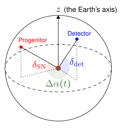
Figure 3: The positions of the detector (blue dot) and the target progenitor (red dot) in our equatorial coordinate system.

We then consider a progenitor whose right ascension and declination are $\alpha_{\rm SN}$ and $\delta_{\rm SN}$, respectively, and define $\Delta\alpha(t)\equiv\alpha_{\rm det}(t)-\alpha_{\rm SN}$, as shown in Fig. 3. In the tangent plane at the detector position, the altitude of the progenitor, $\theta_{\rm SN}(t)$, is given by

$$\sin\theta_{\rm SN}(t)=\cos\delta_{\rm SN}\cos\delta_{\rm det}\cos\Delta\alpha(t)+\sin\delta_{\rm SN}\sin\delta_{\rm det}~{}.$$ (8)

If $|\theta_{\rm SN}|<\theta_{\rm max}$, we can target the SNscope at the progenitor.

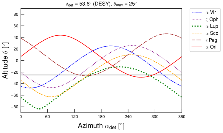
Figure 4: The altitude of the progenitors in Table 1 observed at the detector position $(\alpha_{\rm det},\delta_{\rm det})$ with $\delta_{\rm det}=53.6^{\circ}$ (corresponding to DESY) as functions of $\alpha_{\rm det}$. The horizontal lines correspond to $\theta=\pm\theta_{\rm max}$ with $\theta_{\rm max}=25^{\circ}$.

In Fig. 4, we show the altitude of the progenitors in Table 1 observed at the detector position $(\alpha_{\rm det},\delta_{\rm det})$ with $\delta_{\rm det}=53.6^{\circ}$ (corresponding to DESY) as functions of $\alpha_{\rm det}$. The horizontal lines correspond to $\theta=\pm\theta_{\rm max}$ with $\theta_{\rm max}=25^{\circ}$. From this figure, we see that the observational time fraction $\epsilon_{t}$ is larger than 50% for all of the progenitors in Table 1 except for $\alpha$ Lupi (green dotted line).

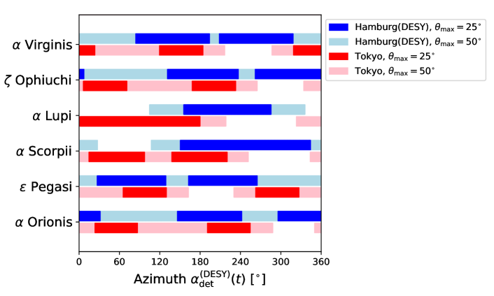
Figure 5: The observable time of each progenitor at DESY and Tokyo ($\delta_{\rm det}=35.7^{\circ}$) in blue and red, respectively, with dark (light) bands corresponding to $\theta_{\rm max}=25^{\circ}$ ($50^{\circ}$). The longitudes of these two points differ by $\simeq 130^{\circ}$.

The effective observational time fractions for these progenitors can be much improved if we simultaneously operate two SNscopes at different observation points or if the maximum elevation $\theta_{\rm max}$ is increased. To see this, in Fig. 5, we show the observable time of each progenitor at DESY and Tokyo ($\delta_{\rm det}=35.7^{\circ}$) in blue and red, respectively, with dark (light) bands corresponding to $\theta_{\rm max}=25^{\circ}$ ($50^{\circ}$). The longitudes of these two points differ by $\simeq 130^{\circ}$. As we see, the axion SNscopes at these two positions complement each other. The extension of the maximum elevation also has significant impact on the observational time fraction; for instance, if IAXO has $\theta_{\rm max}=50^{\circ}$, it can always be directed at $\alpha$ Virginis, $\zeta$ Ophiuchi, $\epsilon$ Pegasi, and $\alpha$ Orionis. Moreover, if both of the SNscopes have $\theta_{\rm max}=50^{\circ}$, then all of the progenitor candidates in Table 1 can always be observed by at least one SNscope.

5.2 Event number

In the first $10$ seconds after the bounce of a core-collapse SN, the axion can be abundantly produced and eventually reach the SNscope on Earth. The dominant production process is the nucleon-nucleon bremsstrahlung in the proto-neutron star,

$$N\,N^{\prime}\rightarrow N\,N^{\prime}+a~{},$$ (9)

where $N$, $N^{\prime}$ can be either proton or neutron. This process was originally calculated in the one-pion exchange (OPE) approximation [93, 94, 16]. However, it was realized that various effects in the nuclear medium can reduce the axion emissivity with respect to the OPE evaluation [95, 96, 19, 20]. To estimate the event number obtained with the SNscope, we follow the result presented in Ref. [20], which considered corrections from the non-vanishing mass of the exchanged pion, the $\rho$ meson exchange, the effective nucleon masses in the medium, and the multiple scattering of nucleons. These effects reduce the axion emissivity from the OPE approximation by about an order of magnitude. The study was done with a simulated $18M_{\odot}$ progenitor and is applicable to heavier SN progenitors with mass $\gtrsim 10M_{\odot}$, such as the SN1987A.

Nevertheless, we emphasize that the result in [20] and thus the event number estimated in this subsection should be considered as a guide rather than a precise evaluation. Besides the uncertainty of the nuclear medium effects, the detail composition of the proto-neutron star remains as an open question [97, 98]. The neglected feedback from the axion emission on the SN further alters the axion emission rate, especially when the axion luminosity is close to that of the neutrino. These effects further obscure the prediction of the axion emissivity from an SN.

We start by showing that the energies of the emitted SN axions are mostly at the $\mathcal{O}$(10) MeV scale. The spectrum of the axions emitted by a unit volume ${\rm d}V$ with temperature $T$ can be expressed as [95, 96]

$$\frac{{{\rm d}}{N}_{a}}{{{\rm d}}\omega{\rm d}t{\rm d}V}=\frac{1}{4{\pi}^{7/2}f_{a}^{2}}\left(\frac{g_{A}}{2f_{\pi}}\right)^{4}n_{B}\rho\;\omega\sqrt{m_{N}T}e^{-\omega/T}s(\omega/T)~{},$$ (10)

where $\omega$ is the energy of the emitted axion, $g_{A}\simeq 1.26$ is the axial charge, $n_{B}$ is the baryon number density, and $\rho$ is the mass density of the unit volume. $s(x)$ is a dimensionless function that depends on the detailed composition of the proto-neutron star medium and the axion-nucleon couplings $C_{N}$. With the normalization of Eq. (10), $s(0)=C_{n}^{2}Y_{n}^{2}+C_{p}^{2}Y_{p}^{2}+\frac{4}{3}Y_{n}Y_{p}(3C_{+}^{2}+C_{-}^{2})$ with the OPE approximation and in the limit of massless pion and non-degenerate nucleon. Here, $Y_{n(p)}$ is the fraction of neutron (proton) and $C_{\pm}\equiv(C_{n}\pm C_{p})$ .

Even though the exact form of $s(x)$ is highly reliant on the uncertain medium effect [20], the shape of the spectrum is only mildly affected. In Fig. 6, we display the scaled axion spectrum $F_{a}(\omega/T)$ from Eq. (10), which is normalized as $\int\!{\rm d}x\,F_{a}(x)=1$, for a unit volume of the SN medium. The dash-dotted and the solid curves represent results obtained with OPE and with medium corrections described in [20], respectively. The red curves are plotted for a schematic uniform SN with temperature $T=30$ MeV, density $\rho=3\times 10^{14}\,{\rm g/cm^{3}}$, and proton fraction $Y_{p}=0.3$ for the KSVZ. The blue curves are plotted with the result from [20] for a simulated SN at a position of $10$ km from the center and $1$s post-bounce. We conclude that the average axion energy is $\langle\omega\rangle\approx(2.2-2.5)\,T$. Over $99.9\%$ of the emitted axions are more energetic than $1$ MeV because of the high SN temperature, and typically have energy of ${\cal O}(10)$ MeV. The momentum dependence of the axion coupling with fermions in Eq. (4) allows the axion to take away large momentum.

Despite the evidently well determined shape of the spectrum, the height of the spectrum remains less understood. After integrating over the axion energy in Eq. (10), the total number of emitted axion scales roughly as $T^{5/2}$ according to dimensional analysis together with the fact that $s(x)$ is almost temperature independent and only a function of $x$. This magnifies the uncertainty from the SN temperature. Moreover, the constituent of the SN and the medium effect can also alter $s(x)$ by an ${\cal O}(1)$ factor; Therefore, we expect roughly an order of magnitude uncertainty in the estimated total number of axion emitted from the SN.

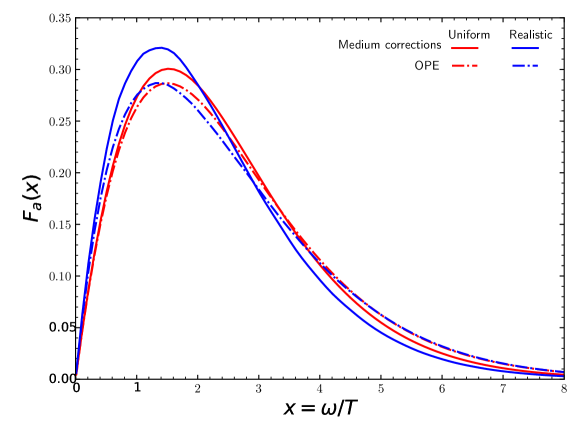
Figure 6: The normalized axion spectrum $F_{a}(\omega/T)$ for a unit volume of the SN medium. The dashed and the solid curves represent the results obtained with OPE and with medium corrections respectively. The red curves are plotted for a schematic uniform SN and the blue curves are plotted for a simulated SN [20].

The axion luminosity of a SN was estimated at the post-bounce time $t_{\rm pb}=1$ s in Ref. [20] as,

$$L_{a}\simeq 2.42\times 10^{70}\,{\rm erg\cdot s^{-1}}\times\left(\frac{m_{N}}{f_{a}}\right)^{2}C_{N,{\rm eff}}^{2}~{},$$ (11)

with

$$C_{N,{\rm eff}}^{2}\equiv C_{n}^{2}+0.61C_{p}^{2}+0.53C_{n}C_{p}~{}.$$ (12)

In the first $10$ s post-bounce, the temperature of the proto-neutron star only varies between $(20-40)$ MeV in its densest region of $r\lesssim 10$ km [97, 20]. For a rough estimation, we approximate the SN as an isothermal object with $T\approx 30$ MeV. The average emitted axion energy is $\langle\omega\rangle\approx 2.3T\approx 70$ MeV. The rate of axion emission is thus,

$$\dot{N}_{a}\simeq\frac{L_{a}}{\langle\omega\rangle}\simeq 2.2\times 10^{74}\,\ {\rm s^{-1}}\times\left(\frac{m_{N}}{f_{a}}\right)^{2}C_{N,{\rm eff}}^{2}~{}.$$ (13)

The probability of an axion converted into a photon inside a helioscope is [29, 99, 100]

$$P=\frac{1}{4}\left(g_{a\gamma\gamma}BL\right)^{2}\left(\frac{\sin\left(qL/2\right)}{qL/2}\right)^{2}~{},$$ (14)

where $q=|m_{a}^{2}-m_{\gamma}^{2}|/(2\omega)$ and $m_{\gamma}$ is the plasma mass of the photon. For maximum conversion of axion to photon, $qL\ll 1$ and $P\approx\left(g_{a\gamma\gamma}BL\right)^{2}/4$. For an evacuated helioscope, $m_{\gamma}=0$ and the maximum axion mass that can be probed efficiently is $m_{a}\lesssim\sqrt{2\omega/L}$. The typical energy of solar axion produced by the Primakoff process is $4$ keV and the helioscopes in Table 2 starts to lose sensitivity when $m_{a}\gtrsim 0.01~{}{\rm eV}$. In contrast, the average SN axion energy is around $70$ MeV and allows the SNscope to probe heavier axions up to $1$ eV.

To summarize, the number of events in the SNscope for $m_{a}\lesssim\sqrt{2\langle\omega\rangle/L}$ is estimated as

$$N \approx P\dot{N}_{a}\ \frac{A}{4\pi d^{2}}\Delta t$$ (15a)

$$\approx 1.0\times\left(\frac{A}{2.3\,{\rm m^{2}}}\right)\left(\frac{B}{2.5\,{\rm T}}\right)^{2}\left(\frac{L}{20\,{\rm m}}\right)^{2}\times\left(\frac{150\,{\rm pc}}{d}\right)^{2}\left(\frac{T}{30\,{\rm MeV}}\right)^{5/2}\left(\frac{\Delta t}{10\,{\rm s}}\right)$$

$$\qquad\times\left(\frac{C_{a\gamma\gamma}}{0.0023}\right)^{2}\left(\frac{3\times 10^{8}\,{\rm GeV}}{f_{a}}\right)^{4}\left(\frac{C_{N,{\rm eff}}}{0.37}\right)^{2}~{},$$ (15b)

while for $m_{a}\gg\sqrt{2\langle\omega\rangle/L}$, the number of events is further suppressed by a factor of $(qL/2)^{-2}$ due to the loss of coherence between the axion and the photon field. $A$, $B$, and $L$ are the helioscope parameters listed in Table 2, $d$ is the distance to the SN, $\Delta t$ is the time of observation, and $C_{a\gamma\gamma}\equiv g_{a\gamma\gamma}f_{a}$. We assume that the detection efficiency of the $\gamma$-ray detector is almost 100%. (See also discussion in Sec. 5.3.) We take $\Delta t\simeq 10$ s since the axion flux remains near its peak value in the first 10s post bounce [97, 20]. In Eq. (15b), we show the scaling of the expected number of events with respect to the properties of the helioscope, the SN and the axion model. In the following discussion, we always assume the SN temperature $T\simeq 30$ MeV for estimation.

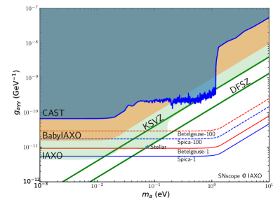
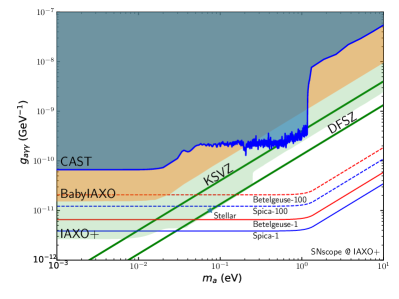
Figure 7: The prospect of the SNscope implemented at IAXO (left) or IAXO+ (right) helioscope with 1 or 100 events for the baseline IAXO SNscope. For illustration we take Spica and Betelgeuse progenitors in Table 1. To obtain the event numbers, we have fixed $C_{N,{\rm eff}}=0.37$ (KSVZ) and $C_{a\gamma\gamma}\equiv g_{a\gamma\gamma}f_{a}=\alpha/\pi$.

In Fig. 7, we plot the contours of 1 and 100 expected events in the $g_{a\gamma\gamma}$-$m_{a}$ plane for the proposed SNscope implemented at IAXO (left panel) or IAXO+ (right panel). The red and the blue contours are plotted respectively for the red supergiant Betelgeuse ($\alpha$ Orionis) and the blue supergiant Spica ($\alpha$ Virginis); the predictions for other progenitors in Table 1 fall between these two curves. To obtain the event numbers, we have fixed the axion parameters at the values in the KSVZ model, $C_{N,{\rm eff}}=0.37$ and $C_{a\gamma\gamma}\equiv g_{a\gamma\gamma}f_{a}=\alpha/\pi$, while taking the axion mass $m_{a}$ as a free parameter. Thus, the event number is proportional to $g_{a\gamma\gamma}^{4}$ in Fig. 7. The event number changes by an ${\cal O}(1)$ factor for different axion models; for instance, for the DFSZ model with $E/N=8/3$, the number increases by a factor of 4 ($\tan\beta\ll 1)$ to 14 $(\tan\beta\gg 1)$. The exclusion region by CAST and the projected exclusion regions by IAXO (as well as BabyIAXO and IAXO+) are taken from [41]. The parameter space for the KSVZ and DFSZ axion models are shown with the green lines. The green asterisk marks the “stellar hint” of the DFSZ axion with $f_{a}=7.7\times 10^{7}\,$GeV and $\tan\beta=0.28$, the best-fit value to the cooling of white dwarfs, red giant branch stars and horizontal branch stars [27]. For $m_{a}<10^{-3}$ eV, the contours remain flat and we ignore this region in the figure. The SNscope starts to lose its sensitivity for $m_{a}\gtrsim 1$ eV due to the loss of coherence between the axion and the photon field. Since the energy of the SN axion is much higher than that of the solar axion, the SNscope probes heavier $m_{a}$ than the helioscopes. This is evident in the region of $m_{a}\gtrsim 0.05$ eV for the DFSZ model which is unreachable by the IAXO helioscope in its buffer gas phase.

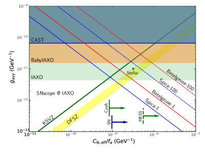
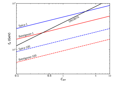
Figure 8: Left panel: the prospect of the SNscope implemented at the IAXO helioscope. For illustration we take Spica and Betelgeuse progenitors in Table 1, and show the contours of 1 (100) event detection by blue and red solid (dashed) lines, respectively. We have fixed $m_{a}=10^{-3}~{}\mbox{eV}$; Right panel: The sensitivity of the SN1987A bound and the 1/100 event contours to the uncertainty of SN axion emission. The latter is parameterized as an overall scaling factor $C_{\rm err}$ to the axion flux.

In the left panel of Fig. 8, we plot similar contours as Fig. 7 but in the plane of $C_{N,\text{eff}}/f_{a}$ and $g_{a\gamma\gamma}$ and with fixed $m_{a}=10^{-3}~{}\mbox{eV}$ for the baseline IAXO SNscope. The green line and the yellow band in this figure represent the relation of $C_{N,\text{eff}}/f_{a}$ and $g_{a\gamma\gamma}$ for the KSVZ and DFSZ axion models, respectively. The projection of the baseline IAXO helioscope covers the parameter space where the QCD axion emitted from a nearby SN gets detected by the IAXO SNscope. If an axion signal is obtained by both the helioscope and the SNscope, it provides valuable structural information of the SN convoluted with the nucleon couplings of the axion. This could be further disentangled in the most optimistic scenario where the event rate in the IAXO helioscope confirms the “stellar hint” of the DFSZ axion.

The dark blue, the green solid and the green dashed arrows in the left panel of Fig. 8 presents the astrophysical bounds on $C_{N,\text{eff}}/f_{a}$ for KSVZ axion from the SN1987A [20], the neutron star in Cas A [22] and the neutron star HESS J1731-347 [23]. These bounds should be regarded as indicators rather than strict constraints since the detail structure and the processes in these stars are not well understood. The cooling processes of neutron stars depend heavily on property of their envelope and the nucleon superfluid in their core. This could lead to ${\cal O}(1)$ uncertainty in the bound. For the SN1987A, a recent study [21] argues that the observed neutrino events might have come from an accretion disk that would not be cooled by axions and this invalidates the bound all together. Even if the SN neutrinos and axions are emitted from the proto-neutron star as in the conventional proposal, the medium effect could still decrease the axion flux [95, 96, 19, 20]. However, this effect both relaxes the SN1987A bound and reduces the expected number of events in the SNscope. We parameterize the uncertainty of the SN axion flux by an overall scaling factor $C_{\rm err}$, so that the “true” axion luminosity and emission rate are parameterized by $\tilde{L}_{a}=C_{\rm err}L_{a}$ and $\dot{\tilde{N}}_{a}=C_{\rm err}\dot{N}_{a}$, with $L_{a}$ and $\dot{N}_{a}$ given by Eq. (11) and Eq. (13) respectively. The SN1987A bound is then set by $\tilde{L}_{a}\lesssim L_{\nu}\simeq 2\times 10^{52}\,{\rm erg}\cdot{\rm s}^{-1}$. For a given axion model, the bound on $f_{a}$ scales as $C_{\rm err}^{1/2}$ while the $f_{a}$ required to observe one event in the SNscope scales as $C_{\rm err}^{1/4}$. This is demonstrated for the KSVZ model in the right panel of Fig. 8. There, the black line depicts the sensitivity of the SN1987A bound on $f_{a}$ to $C_{\rm err}$. The red and the blue solid (dashed) lines are drawn for Spica and Betelgeuse respectively, and represent the $f_{a}$ needed to generate 1 (100) events in the SNscope with varying $C_{\rm err}$. For $C_{\rm err}=0.1$–0.3, the SN1987A observation would be consistent with observing ${\cal O}(10)$ axions from Spica or ${\cal O}(1)$ axions from Betelgeuse with SNscope. Therefore, the observation of axion from a nearby SN is fully plausible even if the SN1987A neutrino was emitted with the conventional mechanism from the proto-neutron star. In any case, the SNscope is a great tool to reserve given the rarity of nearby SN.

5.3 Background estimate

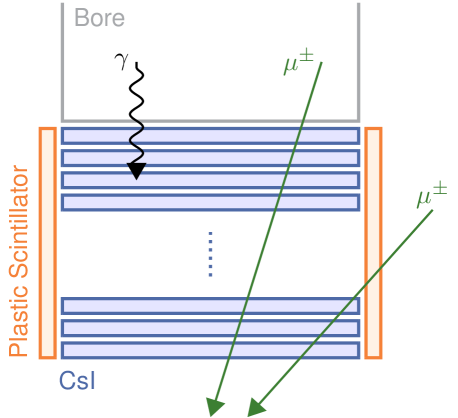
Figure 9: A design for the gamma-ray detector installed on the axion SNscope. The blue and orange rectangles represent CsI and plastic scintillators, respectively.

We now discuss potential background of the axion SNscope. To that end, we consider a concrete setup for the gamma-ray detector, which is illustrated in Fig. 9. We use a set of CsI scintillators (indicated by the blue rectangles) as a gamma-ray detector and pile them up onto the end side of the bore. The side of the detector is surrounded by plastic scintillators (indicated by the orange rectangles), which are used to veto background muons. These scintillators are connected to photosensors to read out scintillation signals. The number of layers of the CsI scintillators will be set large enough so that the photons converted from SN axions deposit most of their energy inside the detector.

The background for SN axion events in this detector is dominantly caused by cosmic-ray muons. The intensity of cosmic-ray muons at sea level is $\sim 1~{}{\rm cm}^{-2}\cdot{\rm min}^{-1}$ [45], and thus for a detector of an ${\cal O}(1)$-meter scale, such as IAXO, we expect $\sim{\cal O}(10^{3})$ muons in $\sim 10$ seconds, which is the typical duration of SN axion burst. It is, therefore, crucial to assure that the detector is able to reject cosmic-ray muons with high accuracy. Hereafter, we focus on muons that pass through the CsI plates perpendicularly, assuming that the plastic scintillators are able to reject muons entering from the side of the detector, as indicated by the right green arrow in Fig. 9, with 100% efficiency.

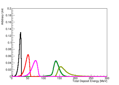
(a) Total Energy deposit.

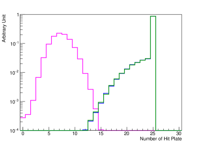
(b) $N_{\rm hit}$

Figure 10: (a) Histograms of the total energy deposit for $30$ MeV (black), $60$ MeV (red), and $90$ MeV (magenta) photons, 0.5 GeV (blue) and 4 GeV (cyan) muons, and 0.5 GeV (green) and 4 GeV (yellow) antimuons; (b) Histograms of the number of plates that receive an energy deposit larger than 1 MeV, $N_{\rm hit}$, for 90 MeV photons (magenta), 0.5 GeV muons (blue), and 0.5 GeV antimuon (green).

To see the prospects for the background muon rejection, we perform Geant4 Monte Carlo simulations [102] using 25 layers of CsI scintillators with a size of $10~{}{\rm cm}\times 10~{}{\rm cm}\times 1~{}{\rm cm}$, which are piled up in parallel and separated by $1$ cm. We generate 2 $\times 10^{5}$ events for 30, 60, and 90 MeV photons and 0.5 GeV and 4 GeV (anti-)muons. All of the particles are injected from above to the center of the top surface of the detector, perpendicularly to the CsI plates. Here 4 GeV muon corresponds to the muon with mean energy at ground level, and 0.5 GeV muon is chosen as a representative of low energy muon.

Figure 10(a) shows the histograms of the total energy deposit for $30$ MeV (black), $60$ MeV (red), and $90$ MeV (magenta) photons, 0.5 GeV (blue) and 4 GeV (cyan) muons, and 0.5 GeV (green) and 4 GeV (yellow) antimuons. It is found that the photons deposit most of their energy inside the detector; we indicate this feature by the black wavy line in Fig. 9. On the other hand, muons and antimuons lose only a small fraction of their initial energy, and thus penetrate through the detector, as shown by the left green arrow in Fig. 9. The total energy deposited by muons scarcely depends on their initial energy and is almost the same as that for antimuons—and is considerably larger than that for photons. We can use this total energy deposit information to eliminate the muon background events.

These muons can also be removed by using the information of the number of plates that receive an energy deposit of more than 1 MeV, $N_{\rm hit}$, as shown in Fig. 10(b). For example, if we apply the selection of $N_{\rm hit}\leq 12$, an ${\cal O}(10^{-4})$ reduction of 0.5 GeV muon is achieved while keeping the $\geq 99.5$% acceptance of the 90 MeV $\gamma$ signal events. Reconstructing the muon trajectory with segmented CsI scintillators also distinguishes signals and backgrounds. The trajectory reconstruction can be improved if the CsI bars are placed perpendicular to each other for neighboring layers. The distribution of energy deposits over the CsI plates may also be useful to distinguish the photon and muon events, even if both the total energy deposit and $N_{\rm hit}$ are similar in these two cases.

A subdominant contribution to the background may be provided by nuclear reactions in the detector material. In particular, neutron captures on nuclei in the detector material emit $\gamma$-rays, which can mimic the signal event. It is, however, found that the energies of such $\gamma$-rays are less than 10 MeV (see, e.g., Ref. [103]), and thus these $\gamma$-rays can be discriminated from the photons converted from SN axions, as can be seen from Fig. 10(a).

All in all, we conclude that it is feasible to sufficiently reduce the number of background events in the axion SNscope, with a realistic setup for the $\gamma$-ray detector. We, therefore, strongly encourage those who work on axion helioscopes to seriously consider the additional installation of such a $\gamma$-ray detector, in order to equip them with the ability of axion SNscopes.

6 Conclusion

If a SN explosion occurs within a few 100 pc from the Earth, it would be a once in a lifetime opportunity for directly detecting SN axions. Together with the high statistics measurements of the SN neutrinos expected for such a nearby SN, the (non-)detection of SN axions will provide valuable information about both the SN and the axion physics. In this paper, we have studied the prospect of directly detecting the SN axions with an axion helioscope equipped with a $\gamma$-ray detector, which we call SNscope. If the $\gamma$-ray detector is installed at the opposite end to the X-ray detector for the solar axion, the experiment still functions as an axion helioscope during the normal operation time, whereas it can work as an axion SNscope once the pre-SN neutrinos alert is received.

There are several nearby SN candidates within hundreds of parsecs. With the help of the pre-SN neutrino events, we may be able to narrow the SN candidates down to a few, or may even uniquely identify the one. An axion SNscope can then be pointed to the (one of) the SN candidate(s) in advance. We have shown that the observation time fraction, i.e., the time fraction when the SNscope can be targeted to a SN progenitor within a day, is larger than 50% for most of the nearby SN candidates, for the IAXO helioscope located at DESY and with a maximal elevation of $\pm\theta_{\rm max}=\pm 25^{\circ}$. The effective observational time fraction significantly increases if two or more SNscopes at different places operate at the same time and/or the maximal elevation $\theta_{\rm max}$ is increased.

The expected number of SN axions detected at a SNscope is estimated in Sec. 5.2, and summarized in Figs. 7 and 8. If a SN explosion occurs within 250 pc, ${\cal O}$(1–100) events can be detected for an axion decay constant $f_{a}\simeq(0.9-5)\times 10^{8}$ GeV taking the KSVZ axion as an example. We have also discussed the background events, in particular the muon background. By combining the veto by the plastic scintillators around the detector, the total energy deposit, and the number of plates with energy deposit, it is feasible that we can sufficiently reduce the number of background events at the axion SNscope.

In summary, our study suggests that the SN axion detection is a realistic and promising option for future axion helioscopes and thus is worth being considered seriously. Further studies, including detailed simulations dedicated to each experimental setup with a concrete design for a $\gamma$-ray detector, are highly motivated, which we leave for future work.

References

- [1] S. Weinberg, A New Light Boson?, Phys. Rev. Lett. 40 (1978) 223–226.
- [2] F. Wilczek, Problem of Strong and Invariance in the Presence of Instantons, Phys. Rev. Lett. 40 (1978) 279–282.
- [3] R. D. Peccei and H. R. Quinn, CP Conservation in the Presence of Instantons, Phys. Rev. Lett. 38 (1977) 1440–1443. [,328(1977)].
- [4] R. D. Peccei and H. R. Quinn, Constraints Imposed by CP Conservation in the Presence of Instantons, Phys. Rev. D16 (1977) 1791–1797.
- [5] J. E. Kim, Weak Interaction Singlet and Strong CP Invariance, Phys. Rev. Lett. 43 (1979) 103.
- [6] M. A. Shifman, A. I. Vainshtein, and V. I. Zakharov, Can Confinement Ensure Natural CP Invariance of Strong Interactions?, Nucl. Phys. B166 (1980) 493–506.
- [7] A. R. Zhitnitsky, On Possible Suppression of the Axion Hadron Interactions. (In Russian), Sov. J. Nucl. Phys. 31 (1980) 260. [Yad. Fiz.31,497(1980)].
- [8] M. Dine, W. Fischler, and M. Srednicki, A Simple Solution to the Strong CP Problem with a Harmless Axion, Phys. Lett. 104B (1981) 199–202.
- [9] Kamiokande-II Collaboration, Observation of a Neutrino Burst from the Supernova SN 1987a, Phys. Rev. Lett. 58 (1987) 1490–1493. [,727(1987)].
- [10] R. M. Bionta et al., Observation of a Neutrino Burst in Coincidence with Supernova SN 1987a in the Large Magellanic Cloud, Phys. Rev. Lett. 58 (1987) 1494.
- [11] E. N. Alekseev, L. N. Alekseeva, V. I. Volchenko, and I. V. Krivosheina, Possible Detection of a Neutrino Signal on 23 February 1987 at the Baksan Underground Scintillation Telescope of the Institute of Nuclear Research, JETP Lett. 45 (1987) 589–592. [,739(1987)].
- [12] J. R. Ellis and K. A. Olive, Constraints on Light Particles From Supernova Sn1987a, Phys. Lett. B193 (1987) 525.
- [13] G. Raffelt and D. Seckel, Bounds on Exotic Particle Interactions from SN 1987a, Phys. Rev. Lett. 60 (1988) 1793.
- [14] M. S. Turner, Axions from SN 1987a, Phys. Rev. Lett. 60 (1988) 1797.
- [15] R. Mayle, et al., Constraints on Axions from SN 1987a, Phys. Lett. B203 (1988) 188–196.
- [16] R. P. Brinkmann and M. S. Turner, Numerical Rates for Nucleon-Nucleon Axion Bremsstrahlung, Phys. Rev. D38 (1988) 2338.
- [17] A. Burrows, M. S. Turner, and R. P. Brinkmann, Axions and SN 1987a, Phys. Rev. D39 (1989) 1020.
- [18] R. Mayle, et al., Updated Constraints on Axions from SN 1987a, Phys. Lett. B219 (1989) 515. [,188(1989)].
- [19] J. H. Chang, R. Essig, and S. D. McDermott, Supernova 1987A Constraints on Sub-GeV Dark Sectors, Millicharged Particles, the QCD Axion, and an Axion-like Particle, JHEP 09 (2018) 051 [arXiv:1803.00993].
- [20] P. Carenza, et al., Improved axion emissivity from a supernova via nucleon-nucleon bremsstrahlung, JCAP 1910 (2019) 016 [arXiv:1906.11844].
- [21] N. Bar, K. Blum, and G. D’amico, Is there a supernova bound on axions?, Phys. Rev. D 101 (2020) 123025 [arXiv:1907.05020].
- [22] K. Hamaguchi, N. Nagata, K. Yanagi, and J. Zheng, Limit on the Axion Decay Constant from the Cooling Neutron Star in Cassiopeia A, Phys. Rev. D98 (2018) 103015 [arXiv:1806.07151].
- [23] M. V. Beznogov, E. Rrapaj, D. Page, and S. Reddy, Constraints on Axion-like Particles and Nucleon Pairing in Dense Matter from the Hot Neutron Star in HESS J1731-347, Phys. Rev. C98 (2018) 035802 [arXiv:1806.07991].
- [24] L. B. Leinson, Constraints on axions from neutron star in HESS J1731-347, JCAP 2019 (2019) 031 [arXiv:1909.03941].
- [25] G. G. Raffelt, J. Redondo, and N. Viaux Maira, The meV mass frontier of axion physics, Phys. Rev. D84 (2011) 103008 [arXiv:1110.6397].
- [26] M. Giannotti, I. Irastorza, J. Redondo, and A. Ringwald, Cool WISPs for stellar cooling excesses, JCAP 05 (2016) 057 [arXiv:1512.08108].
- [27] M. Giannotti, I. G. Irastorza, J. Redondo, A. Ringwald, and K. Saikawa, Stellar Recipes for Axion Hunters, JCAP 1710 (2017) 010 [arXiv:1708.02111].
- [28] K. Saikawa and T. T. Yanagida, Stellar cooling anomalies and variant axion models, JCAP 03 (2020) 007 [arXiv:1907.07662].
- [29] P. Sikivie, Experimental Tests of the Invisible Axion, Phys. Rev. Lett. 51 (1983) 1415–1417. [Erratum: Phys.Rev.Lett. 52, 695 (1984)].
- [30] D. M. Lazarus, et al., A Search for solar axions, Phys. Rev. Lett. 69 (1992) 2333–2336.
- [31] S. Moriyama, et al., Direct search for solar axions by using strong magnetic field and x-ray detectors, Phys. Lett. B434 (1998) 147 [hep-ex/9805026].
- [32] Y. Inoue, et al., Search for sub-electronvolt solar axions using coherent conversion of axions into photons in magnetic field and gas helium, Phys. Lett. B536 (2002) 18–23 [astro-ph/0204388].
- [33] Y. Inoue, et al., Search for solar axions with mass around 1 eV using coherent conversion of axions into photons, Phys. Lett. B668 (2008) 93–97 [arXiv:0806.2230].
- [34] CAST Collaboration, First results from the CERN Axion Solar Telescope (CAST), Phys. Rev. Lett. 94 (2005) 121301 [hep-ex/0411033].
- [35] CAST Collaboration, An Improved limit on the axion-photon coupling from the CAST experiment, JCAP 0704 (2007) 010 [hep-ex/0702006].
- [36] CAST Collaboration, Probing eV-scale axions with CAST, JCAP 0902 (2009) 008 [arXiv:0810.4482].
- [37] CAST Collaboration, CAST search for sub-eV mass solar axions with 3He buffer gas, Phys. Rev. Lett. 107 (2011) 261302 [arXiv:1106.3919].
- [38] CAST Collaboration, Search for Solar Axions by the CERN Axion Solar Telescope with 3He Buffer Gas: Closing the Hot Dark Matter Gap, Phys. Rev. Lett. 112 (2014) 091302 [arXiv:1307.1985].
- [39] CAST Collaboration, New CAST Limit on the Axion-Photon Interaction, Nature Phys. 13 (2017) 584–590 [arXiv:1705.02290].
- [40] E. Armengaud et al., Conceptual Design of the International Axion Observatory (IAXO), JINST 9 (2014) T05002 [arXiv:1401.3233].
- [41] IAXO Collaboration, Physics potential of the International Axion Observatory (IAXO), JCAP 1906 (2019) 047 [arXiv:1904.09155].
- [42] TASTE Collaboration, Towards a medium-scale axion helioscope and haloscope, JINST 12 (2017) P11019 [arXiv:1706.09378].
- [43] P. Antonioli et al., SNEWS: The Supernova Early Warning System, New J. Phys. 6 (2004) 114 [astro-ph/0406214].
- [44] I. G. Irastorza and J. Redondo, New experimental approaches in the search for axion-like particles, Prog. Part. Nucl. Phys. 102 (2018) 89–159 [arXiv:1801.08127].
- [45] Particle Data Group Collaboration, Review of Particle Physics, Phys. Rev. D98 (2018) 030001.
- [46] L. Di Luzio, M. Giannotti, E. Nardi, and L. Visinelli, The landscape of QCD axion models, arXiv:2003.01100 (2020).
- [47] P. Sikivie, Invisible Axion Search Methods, arXiv:2003.02206 (2020).
- [48] M. Gorghetto and G. Villadoro, Topological Susceptibility and QCD Axion Mass: QED and NNLO corrections, JHEP 03 (2019) 033 [arXiv:1812.01008].
- [49] S. Borsanyi et al., Calculation of the axion mass based on high-temperature lattice quantum chromodynamics, Nature 539 (2016) 69–71 [arXiv:1606.07494].
- [50] G. Grilli di Cortona, E. Hardy, J. Pardo Vega, and G. Villadoro, The QCD axion, precisely, JHEP 01 (2016) 034 [arXiv:1511.02867].
- [51] F. Capozzi and G. Raffelt, Axion and neutrino red-giant bounds updated with geometric distance determinations, arXiv:2007.03694 (2020).
- [52] P. Carenza, et al. in 14th Patras Workshop on Axions, WIMPs and WISPs. 2018. arXiv:1808.04101.
- [53] P. Carenza, AXION EMISSION AND DETECTION FROM A GALACTIC SUPERNOVA, http://www.dmf.unisalento.it/~gpco/tesi/TesiPCarenza.pdf, 2018. Ph.D. Thesis.
- [54] M. Meyer, M. Giannotti, A. Mirizzi, J. Conrad, and M. A. Sánchez-Conde, Fermi Large Area Telescope as a Galactic Supernovae Axionscope, Phys. Rev. Lett. 118 (2017) 011103 [arXiv:1609.02350].
- [55] M. Meyer and T. Petrushevska, Search for Axionlike-Particle-Induced Prompt Gamma-Ray Emission from Extragalactic Core-Collapse Supernovae with the Fermi Large Area Telescope, Phys. Rev. Lett. 124 (2020) 231101 [arXiv:2006.06722].
- [56] A. Odrzywolek, M. Misiaszek, and M. Kutschera, Detection possibility of the pair - annihilation neutrinos from the neutrino - cooled pre-supernova star, Astropart. Phys. 21 (2004) 303–313 [astro-ph/0311012].
- [57] A. Odrzywolek, M. Misiaszek, and M. Kutschera, Neutrinos from pre-supernova star, Acta Phys. Polon. B35 (2004) 1981 [astro-ph/0405006].
- [58] M. Kutschera, A. Odrzywołek, and M. Misiaszek, Presupernovae as Powerful Neutrino Sources, Acta Physica Polonica B 40 (2009) 3063.
- [59] A. Odrzywolek, Nuclear statistical equilibrium neutrino spectrum, Phys. Rev. C80 (2009) 045801 [arXiv:0903.2311].
- [60] C. Kato, et al., Pre-supernova neutrino emissions from ONe cores in the progenitors of core-collapse supernovae: are they distinguishable from those of Fe cores?, Astrophys. J. 808 (2015) 168 [arXiv:1506.02358].
- [61] K. M. Patton, C. Lunardini, and R. J. Farmer, Presupernova neutrinos: realistic emissivities from stellar evolution, Astrophys. J. 840 (2017) 2 [arXiv:1511.02820].
- [62] T. Yoshida, K. Takahashi, H. Umeda, and K. Ishidoshiro, Presupernova neutrino events relating to the final evolution of massive stars, Phys. Rev. D93 (2016) 123012 [arXiv:1606.04915].
- [63] C. Kato, et al., Neutrino emissions in all flavors up to the pre-bounce of massive stars and the possibility of their detections, Astrophys. J. 848 (2017) 48 [arXiv:1704.05480].
- [64] K. M. Patton, C. Lunardini, R. J. Farmer, and F. X. Timmes, Neutrinos from beta processes in a presupernova: probing the isotopic evolution of a massive star, Astrophys. J. 851 (2017) 6 [arXiv:1709.01877].
- [65] G. Guo, Y.-Z. Qian, and A. Heger, Presupernova neutrino signals as potential probes of neutrino mass hierarchy, Phys. Lett. B796 (2019) 126–130 [arXiv:1906.06839].
- [66] C. Kato, K. Ishidoshiro, and T. Yoshida, Theoretical prediction of presupernova neutrinos and their detection, arXiv:2006.02519 (2020).
- [67] KamLAND Collaboration, KamLAND Sensitivity to Neutrinos from Pre-Supernova Stars, Astrophys. J. 818 (2016) 91 [arXiv:1506.01175].
- [68] SNO+ Collaboration, Current Status and Future Prospects of the SNO+ Experiment, Adv. High Energy Phys. 2016 (2016) 6194250 [arXiv:1508.05759].
- [69] Super-Kamiokande Collaboration, Sensitivity of Super-Kamiokande with Gadolinium to Low Energy Anti-neutrinos from Pre-supernova Emission, Astrophys. J. 885 (2019) 133 [arXiv:1908.07551].
- [70] Hyper-Kamiokande Collaboration, Hyper-Kamiokande Design Report, arXiv:1805.04163 (2018).
- [71] JUNO Collaboration, Neutrino Physics with JUNO, J. Phys. G43 (2016) 030401 [arXiv:1507.05613].
- [72] DUNE Collaboration, The DUNE Far Detector Interim Design Report Volume 1: Physics, Technology and Strategies, arXiv:1807.10334 (2018).
- [73] DUNE Collaboration, Deep Underground Neutrino Experiment (DUNE), Far Detector Technical Design Report, Volume II DUNE Physics, arXiv:2002.03005 (2020).
- [74] N. Raj, V. Takhistov, and S. J. Witte, Presupernova neutrinos in large dark matter direct detection experiments, Phys. Rev. D101 (2020) 043008 [arXiv:1905.09283].
- [75] K. Scholberg, The SuperNova Early Warning System, Astron. Nachr. 329 (2008) 337–339 [arXiv:0803.0531].
- [76] SNEWS Collaboration, SNEWS: The supernova early warning system, J. Phys. Conf. Ser. 309 (2011) 012026.
- [77] S. BenZvi, SNEWS 2.0: A Supernova Early Warning System for the Multimessenger Era, https://indico.cern.ch/event/868940/contributions/3813639/attachments/2081550/3496381/BenZvi_SNEWS_2.0.pdf, 2020. Talk at ICHEP 2020, Jul. 28–Aug. 6, 2020.
- [78] F. van Leeuwen, Validation of the new Hipparcos reduction, Astron. Astrophys. 474 (2007) 653–664 [arXiv:0708.1752].
- [79] A. Tkachenko, et al., Stellar modelling of Spica, a high-mass spectroscopic binary with a Cep variable primary component, Mon. Not. Roy. Astron. Soc. 458 (2016) 1964–1976 [arXiv:1601.08069].
- [80] I. D. Howarth and K. C. Smith, Rotational mixing in early-type main-sequence stars, Mon. Not. Roy. Astron. Soc. 327 (2001) 353–368.
- [81] N. Tetzlaff, R. Neuhäuser, and M. M. Hohle, A catalogue of young runaway Hipparcos stars within 3 kpc from the Sun, Mon. Not. Roy. Astron. Soc. 410 (2011) 190–200 [arXiv:1007.4883].
- [82] K. Ohnaka, et al., High spectral resolution imaging of the dynamical atmosphere of the red supergiant Antares in the CO first overtone lines with VLTI/AMBER, Astron. Astrophys. 555 (2013) A24 [arXiv:1304.4800].
- [83] G. M. Harper, et al., An Updated 2017 Astrometric Solution for Betelgeuse, Astron. J. 154 (2017) 11 [arXiv:1706.06020].
- [84] H. R. Neilson, J. B. Lester, and X. Haubois in 9th Pacific Rim Conference on Stellar Astrophysics, S. Qain, et al., eds., vol. 451 of Astronomical Society of the Pacific Conference Series, p. 117. 2011. arXiv:1109.4562.
- [85] K. Nakamura, et al., Multimessenger signals of long-term core-collapse supernova simulations: synergetic observation strategies, Mon. Not. Roy. Astron. Soc. 461 (2016) 3296–3313 [arXiv:1602.03028].
- [86] List of nearby RSG candidates, http://th.nao.ac.jp/MEMBER/nakamura/2016multi/.
- [87] M. Mukhopadhyay, C. Lunardini, F. X. Timmes, and K. Zuber, Presupernova neutrinos: directional sensitivity and prospects for progenitor identification, arXiv:2004.02045 (2020).
- [88] N. Panagia, et al., Photometric properties of SN 1987A and other sources in the same field., Astron. Astrophys. 177 (1987) L25–L28.
- [89] R. Gilmozzi, et al., The progenitor of SN1987A, Nature 328 (1987) 318–320.
- [90] G. Sonneborn, B. Altner, and R. P. Kirshner, The Progenitor of SN 1987A: Spatially Resolved Ultraviolet Spectroscopy of the Supernova Field, Astrophys. J. Lett. 323 (1987) L35.
- [91] H.-L. Li, Y.-F. Li, L.-J. Wen, and S. Zhou, Prospects for Pre-supernova Neutrino Observation in Future Large Liquid-scintillator Detectors, JCAP 05 (2020) 049 [arXiv:2003.03982].
- [92] H. K. M. Tanaka and H. Watanabe, 6Li-loaded directionally sensitive anti-neutrino detector for possible geo-neutrinographic imaging applications, Scientific Reports 4 (2014) 4708.
- [93] N. Iwamoto, Axion Emission from Neutron Stars, Phys. Rev. Lett. 53 (1984) 1198–1201.
- [94] M. S. Turner, Axions, SN 1987a and One Pion Exchange, Phys. Rev. D 40 (1989) 299–308.
- [95] G. Raffelt and D. Seckel, A selfconsistent approach to neutral current processes in supernova cores, Phys. Rev. D 52 (1995) 1780–1799 [astro-ph/9312019].
- [96] S. Hannestad and G. Raffelt, Supernova neutrino opacity from nucleon-nucleon Bremsstrahlung and related processes, Astrophys. J. 507 (1998) 339–352 [astro-ph/9711132].
- [97] T. Fischer, et al., Probing axions with the neutrino signal from the next galactic supernova, Phys. Rev. D 94 (2016) 085012 [arXiv:1605.08780].
- [98] T. Sukhbold, T. Ertl, S. E. Woosley, J. M. Brown, and H. T. Janka, Core-Collapse Supernovae from 9 to 120 Solar Masses Based on Neutrino-powered Explosions, Astrophys. J. 821 (2016) 38 [arXiv:1510.04643].
- [99] P. Sikivie, Detection Rates for ’Invisible’ Axion Searches, Phys. Rev. D 32 (1985) 2988. [Erratum: Phys.Rev.D 36, 974 (1987)].
- [100] G. Raffelt and L. Stodolsky, Mixing of the Photon with Low Mass Particles, Phys. Rev. D 37 (1988) 1237.
- [101] CAST Collaboration, New solar axion search using the CERN Axion Solar Telescope with 4He filling, Phys. Rev. D 92 (2015) 021101 [arXiv:1503.00610].
- [102] S. Agostinelli, et al., Geant4—a simulation toolkit, Nuclear Instruments and Methods in Physics Research Section A: Accelerators, Spectrometers, Detectors and Associated Equipment 506 (2003) 250 – 303.
- [103] T. Iida et al., The energy calibration system for CANDLES using (, ) reaction, arXiv:2003.13404 (2020).