Characterizing The Many-Body Localization via Studying State Sensitivity to Boundary Conditions

Abstract

We introduce novel characterizations for many-body phase transitions between delocalized and localized phases based on the system’s sensitivity to boundary conditions. In particular, we change boundary conditions from periodic to antiperiodic and calculate shift in the system’s energy and shifts in the single-particle density matrix eigenvalues in the corresponding energy window. We employ the typical model for studying MBL, a one-dimensional disordered system of fermions with nearest-neighbor repulsive interaction where disorder is introduced as randomness on on-site energies. By calculating numerically the shifts in the system’s energy and eigenvalues of the single-particle density matrix, we observe that in the localized regime, both shifts are vanishing; while in the extended regime, both shifts are on the order of the corresponding level spacing. We also applied these characterizations of the phase transition to the case of having next-nearest-neighbor interactions in addition to the nearest-neighbor interactions, and studied its effect on the transition.

I Introduction

In a free fermion model with extending plain-wave eigenfunctions, fermions move freely in the entire system. Introducing randomness in the free fermion model, which represents disorder, leads to the localization of fermions due to the quantum interference, proposed by AndersonAnderson (1958). This phenomenon, so-called Anderson localization, has been widely studied numerically, analytically, and experimentally. In general, the Anderson localization is associated with the symmetry and dimension of the systemHorodecki et al. (2009). For one- and two-dimensional systems, any infinitesimal uncorrelated randomness makes the system localizedEvers and Mirlin (2008). For a three-dimensional (3D) system, however, there exists a non-zero critical disorder strength at which a quantum phase transition between localized and delocalized phase occursMacKinnon and Kramer (1981). In a weak randomness regime, system is delocalized; as the disorder strength increases and hits the critical value, the system becomes localized. Besides, a phase transition from a delocalized to a localized phases can be seen in the energy resolution, if the system under study has mobility edges. A 3D Anderson model, for example, has localized phases at both tails of the energy spectrum, and delocalized phases in the middle of the spectrumEconomou and Cohen (1972); Izrailev and Krokhin (1999). Thus, as the system’s energy changes from one energy window to another, it will undergo a phase transition between localized and delocalized phases.

Another interesting phenomenon arises when interaction is introduced in the Anderson model, whence we encounter the following questions: Does disorder suppress the effect of the interaction? or interaction effect is so strong that makes the interacting system delocalized? More interestingly, what role does temperature play in such a system? We can also ask these questions from the perspective of statistical physics: It is assumed that a classical ergodic system can visit its whole phase space after a finite time, so the averaging a physical quantity over time is the same as averaging over the whole phase space. In this perspective, the question of the ergodicity of a random interacting system is importantNandkishore and Huse (2015). Answering the above questions is one of the hot research topics. By now, we know that in the interacting systems, at a non-zero temperature, a phase transition between localized and delocalized phases arises by varying disorder strengthAltman (2018); Abanin et al. (2019). In strong disorder regime, the conductivity– even at a non-zero temperature– is zero, and the state of the system is localized in Fock space. The phase is thus called many-body localized (MBL) phaseBasko et al. (2006); Parameswaran et al. (2017); Alet and Laflorencie (2018); Altman and Vosk (2015). The states in the MBL phase do not thermalize in the sense that after a long time, its properties still depend on the initial state of the system (i.e. local integrals of motion constrain the system); in other words, the system carries the information of the initial statesNandkishore and Huse (2015). Thus, an MBL phase is an out-of-equilibrium phase, and the laws of statistical mechanics are not obeyed. On the other hand, in weak disorder regime, a part of the system acts as a bath for the remainder, such that the eigenstate thermalization hypothesis (ETH)Deutsch (1991); Srednicki (1994); Rigol et al. (2008); Deutsch (2018) can be applied, and the system thermalizes. In addition, an ETH-MBL phase transition can be seen at a fixed disorder strength in the energy resolution, i.e. the mobility edges can also be seen in the interacting systemBaygan et al. (2015); Li et al. (2015).

Experimentally, phase transition between the ETH and MBL phases has been witnessed in many systems such as ultra-cold atomsBloch et al. (2008), trapped ions systems Smith et al. (2016), optical latticesLangen et al. (2015); Chin et al. (2010); Kaufman et al. (2016); Bordia et al. (2017); Choi et al. (2016); Bordia et al. (2016); Schreiber et al. (2015), and quantum information devicesSapienza et al. (2010).

In the remainder of this section, we first cite models with ETH-MBL phase transitions. Then we mention some of the previously studied ETH-MBL phase transition characterizations along with our novel characterization. The typical model employed to study the ETH-MBL phase transition is the spinless fermion model with constant nearest-neighbor (NN) hopping and NN interactions (which is the Jordan-Wigner transformation of the XXZ model for the spin $1/2$); disorder is introduced by random on-site energies. Some studies also introduced random interactions into the systemPapić et al. (2015); Li et al. (2017); Bar Lev et al. (2016). Having MBL phase in translation-invariant Hamiltonians and systems with delocalized single-particle spectrum, also have been investigatedYao et al. (2016); Bar Lev et al. (2016); Smith et al. (2017); De Roeck and Huveneers (2014). Although disorder is usually described by random on-site energies, some studies reported that on-site energies with incommensurate periodicity could trigger ETH-MBL phase transitionsLi et al. (2015); Modak and Mukerjee (2015); Li et al. (2016); other systems such as a frustrated spin chainChoudhury et al. (2018) and a system under strong electric fieldSchulz et al. (2019) also exhibit ETH-MBL phase transitions.

Finding a characterization for the ETH-MBL phase transition is part of the current research. Entanglement entropy (EE) is one candidate that shows distinguished behavior in the ETH and MBL phasesKjäll et al. (2014); Geraedts et al. (2017). To calculate EE, one divides the system into two subsystems $A$ and $B$; reduced density matrix of each subsystem $\rho_{A/B}$ is calculated by tracing over degrees of freedom of other subsystem. EE then can be calculated as $\text{EE}=-tr\rho_{A/B}\log\rho_{A/B}$ Horodecki et al. (2009); Laflorencie (2016). EE follows an area-law behavior in the MBL phaseBardarson et al. (2012); Serbyn et al. (2013); while it obeys volume law in the ETH phase, where the reduced density matrix of a subsystem approaches the thermal density matrix. EE thus fluctuates strongly around the localization-delocalization transition pointKhemani et al. (2017). In addition, the statistics of the low energy entanglement spectrum (eigenvalues of the reduced density matrix) has been used as a characterization of the phase transition. The entanglement spectrum distribution goes from Gaussian orthogonal in extended regime to a Poisson distribution in localized regimeRichard . Furthermore, people have used the eigen-energies level spacingOganesyan and Huse (2007) and level dynamicsMaksymov et al. (2019) as characterizations. Some other methods, such as machine learning is also used for detecting the MBL phase transitionRao (2018). These were just to name a few, among many othersFilippone et al. (2016); Li et al. (2016); Richard ; De Luca et al. (2014); Li et al. (2015).

A recent paperBera et al. (2015) studied the single-particle density matrix to distinguish MBL from the ETH phase. The single-particle density matrices are constructed by the eigenstates of the Hamiltonian ($H$) of the system in a target energy window through

$$\centering\rho_{ij}=\langle\psi|c^{\dagger}_{i}c_{j}|\psi\rangle,\@add@centering$$ (1)

where $i$ and $j$ go from $1$ to $L$ (system size), and $|\psi\rangle$ is the eigenstate of the Hamiltonian. They studied eigenvalues $\{n\}$ and eigenfunctions of the density matrix, $|\phi_{k}\rangle$. Its eigenvalues, which can be interpreted as occupations of the orbitals, demonstrate the Fock space localization: Deep in the delocalized phase, $\{n\}$’s are evenly spaced between $0$ and $1$. While, in the localized phase, they tend to be very close to either $0$ or $1$. Thus, the difference between two successive eigenvalues of $\rho$ shows different behavior in delocalized and localized phases. Moreover, they found that eigenfunctions of the density matrix, $|\phi_{k}\rangle$ are extended (localized) in delocalized (localized) phaseBera et al. (2017); Lin et al. (2018).

We, in this paper, look at the ETH-MBL phase transition from the perspective of boundary condition effects on the system, namely, we change the boundary conditions from periodic to antiperiodic and then study its effects on the system’s energy as well as on the eigenvalues of the single-particle density matrix ($\rho$) at a given energy window (see section II for more detail). Our work is a generalization of Ref. [Edwards and Thouless, 1972] where Anderson localization in free fermion models is characterized based on the response of the system to the change in the boundary conditions. The response of an interacting system to a local perturbation, on the other hand, is also investigated in Refs. [Serbyn et al., 2017; Khemani et al., 2015] as a characterization of the MBL phase, which is analogous to our work.

Results of our work, in brief, are as follows. In contrast to the MBL phase, the system’s energy and occupation numbers are sensitive to the boundary conditions in the ETH phase. In MBL phase, shifts in the system’s energy and occupation numbers are vanishing; however, in ETH phase, both shifts are on the order of the corresponding level spacing. We use these metrics in a previously studied model with NN interactions that has a known ETH-MBL phase transition. We also apply these characterizations to a model having both NN and NNN interactions.

The paper’s structure is as follows; We first introduce the model and explain the numerical method in section II. The responses of the Hamiltonian’s eigen-energy and the single-particle density matrix eigenvalues to the boundary conditions, considering only the NN interaction, will be presented in sections III and IV, respectively. In sec V, we introduce the NNN interaction in the model and consider its effect. We close with some remarks in section VI.

II Method and Model

We consider spinless fermions confined on a one-dimensional (1D) chain with the nearest-neighbor (NN) hopping; NN and next-nearest-neighbor (NNN) repulsive density-density interactions as well as diagonal disorder. The effective Hamiltonian can be written as:

$$H =-t\sum_{i=1}^{L}\left(c_{i}^{\dagger}c_{i+1}+h.c.\right)+\sum_{i=1}^{L}\mu_{i}(n_{i}-\frac{1}{2})$$ (2)

$$+ V_{1}\sum_{i=1}^{L}(n_{i}-\frac{1}{2})(n_{i+1}-\frac{1}{2})+V_{2}\sum_{i=1}^{L}(n_{i}-\frac{1}{2})(n_{i+2}-\frac{1}{2}).$$

where $c_{i}^{\dagger}(c_{i})$ is the fermionic creation (annihilation) operator, creating (annihilating) a fermion on the site $i$ and $n_{i}=c^{\dagger}_{i}c_{i}$ is the number operator. The first term in the Hamiltonian is the NN hopping with constant strength $t$, which is used as the energy unit in our calculations and is set to unity. The randomized on-site energies, as a disorder representation, are described by $\mu$’s. They follow uniform distribution within $[-W,W]$, where $W$ is called disorder strength. The last two terms in the Hamiltonian are the constant repulsive NN and NNN density-density interactions.

To apply boundary conditions, we set $c^{(\dagger)}_{i+L}=c^{(\dagger)}_{i}$ for the the periodic boundary condition (PBC) and $c^{(\dagger)}_{i+L}=-c^{(\dagger)}_{i}$ for the antiperiodic boundary condition (APBC) where $L$ is the length of the 1D chain.

We first diagonalize the Hamiltonian through exact diagonalization method, and find its eigenvectors and the corresponding eigenvalues. We use parameter $\epsilon$ which is defined as $\epsilon=\frac{(E-E_{0})}{(E_{max}-E_{0})}$, where $E$ is the target energy, $E_{0}$ is the ground state energy, and $E_{max}$ represents the highest energy in the spectrum; it changes between $0$ and $1$ corresponding to the ground state and highest energy, respectively. We focus on a certain energy window of the spectrum: For a given $\epsilon$, we calculate the target energy $E$ and select six eigenstates of $H$ with the energy closest to $E$. For each of these six eigenstates, we build up the single-particle density matrix $\rho$ from Eq. (1). By changing the boundary conditions from PBC to APBC, we calculate the energy shift for each eigenstate:

$$\delta E_{i}=|E_{i,PBC}-E_{i,APBC}|,$$ (3)

where $E_{i}$ is the energy of the $i$th eigenstate; in this way, $i$th level of the Hamiltonian with PBC is compared with the $i$th level of the Hamiltonian with APBC. We then take typical averaging over six eigenstates and take typical disorder average to obtain $\delta E^{typ}$ (typical average of random variable $x$ is $e^{\langle\ln x\rangle}$, where $\langle\cdots\rangle$ stands for arithmetic mean). In the same manner, we calculate shifts in the eigenvalues of the single-particle density matrix:

$$\delta n_{i}^{(j)}=|n_{i,PBC}^{(j)}-n_{i,APBC}^{(j)}|.$$ (4)

A typical average on all eigenvalues of the $\rho$ ($j$ goes from $1$ to $L$), another typical average over the six samples, and a typical disorder average will be calculated to obtain $\delta n^{typ}$.

III Effect of the boundary change on the energy

In a free fermion model, the state of the system is the Slater determinant of the occupied single-particle eigenstates. In the localized phase, occupied eigenstates of the system are confined in a small region of space, while in the delocalized phase, they spread over entire system. In Ref. [Edwards and Thouless, 1972], the effect of the change in the boundary conditions on the single-particle eigen-energies of a free fermion model is studied. By changing the boundary conditions in the localized phase, the single-particle energy does not change. On the other hand, in the delocalized phase, where eigenstates of the system are extended, any changes in the boundary conditions can be seen by the wave-function; these changes are then reflected in the corresponding energy. Accordingly, the energy shift for each level, $\delta E$, divided by the average level spacing $\Delta E$ known as Thouless conductance, is a characterization of the Anderson phase transition between delocalized and localized phases:

$$\centering g_{E}=\delta E/\Delta E.\@add@centering$$ (5)

We conjecture that if we change boundary conditions for an interacting system, a similar quantity as Thouless conductance (now for the system’s energy rather than the single-particle eigen-energy) can be used to characterize the phase transition. In particular, we change the condition from periodic to antiperiodic (as explained in section II) and calculate $g_{E}$ for the system’s energy. In Fig. 1, typical averaged $g_{E}$ is plotted for some selected values of the energy for the case of NN interaction of Eq. (2) corresponding to $V_{1}=1,V_{2}=0$ (standard deviation of $g_{E}$ is plotted in Fig. 7). We see that deep in the delocalized phase, the shift in the system’s energy is on the order of level spacing, while deep in the localized phase, the shift is zero. Based on this plot, in the middle of the spectrum ($\epsilon=0.5$), $g_{E}$ goes to zero at $W\approx 3.5$, consistent with the previously obtained resultsLuitz et al. (2015); Serbyn et al. (2017); Filho et al. (2017); Villalonga et al. (2018). Also, $g_{E}$ is plotted for the whole spectrum of energy in Fig. 2 as we vary the disorder strength $W$. This plot is also consistent with the previously obtained results.

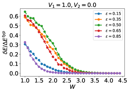
Figure 1: (color online) typical averaged $g_{E}=\frac{\delta E}{\Delta E}$ for the case of having only NN interaction ($V_{1}=1,V_{2}=0$) for some selected $\epsilon$ as disorder strength $W$ varies. We set $L=14,N=7$. We take typical disorder average over altogether $2000$ samples for each data point.

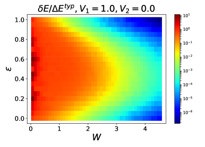
Figure 2: (color online) typical average of $g_{E}=\frac{\delta E}{\Delta E}$ for the entire spectrum of the energy as we change the disorder strength $W$ for the NN interaction case ($V_{1}=1,V_{2}=0$). System size $L=14,N=7$. We take typical disorder average over altogether $2000$ samples for each data point.

IV Effect of the boundary change on the single-particle density matrix

Now, we focus on the effect of boundary conditions on the occupation numbers of density matrix Eq. (1). First, let us look at the case of free fermions, where we can write the Hamiltonian of the system as:

$$\centering H_{\text{Free fermion}}=\sum_{i,j=1}^{L}h_{ij}\ c^{\dagger}_{i}c_{j},\@add@centering$$ (6)

we observe that eigen-functions of the single-particle density matrix and matrix $h$ are the same (both can be diagonalized by the same unitary matrix):

$$\centering h_{ij}\@add@centering = \sum_{k}U_{ik}\ \epsilon_{k}\ U_{kj}^{\dagger},$$ (7)

$$\rho_{ij} = \sum_{k}U_{ik}\ n_{k}\ U_{kj}^{\dagger},$$ (8)

where $\epsilon_{k}$ is the single-particle eigen-energy of the Hamiltonian. By the argument of ThoulessEdwards and Thouless (1972) that single-particle eigenstates of the Hamiltonian are sensitive (insensitive) to the boundary conditions in delocalized (localized) phase, we can say that eigenvalues of the $\rho$ are sensitive (insensitive) to the boundary conditions in delocalized (localized) phase. Thus, we can identify the shifts in the eigenvalues of the $\rho$ when we change the boundary condition from periodic to antiperiodic as a probe of the phase transition.

This idea has been verified indirectly before: We know that for a free fermion system divided into two subsystems, reduced density matrix of each subsystem can be written as $\exp(-H_{\text{ent}})$, where $H_{\text{ent}}$ is called entanglement Hamiltonian and can be obtained from single-particle density matrix of the corresponding subsystemPeschel (2003). Effect of the boundary condition changes on the entanglement Hamiltonian for free fermion models was studied in Ref [Pouranvari and Montakhab, 2017]: Boundary condition is changed from periodic to antiperiodic and shifts in the eigenvalues of the entanglement Hamiltonian (and thus on the entanglement entropy) are calculated; and it is shown that they can be used as characterization of the localized-delocalized phase transition.

For the interacting case, we know that the single-particle density matrix eigenstates are localized (delocalized) in the localized (delocalized) phaseBera et al. (2015); Thus, we put one step forwards and conjecture that ETH phase can be distinguished from the MBL phase by analyzing the shifts of the occupation numbers when we change boundary conditions. In particular, we change the boundary condition from periodic to antiperiodic (as described in Section II) and calculate the shifts in the occupation numbers of single-particle density matrix $\delta n$.

In Fig. 3 we plot occupation numbers for the NN interaction case of Eq. (2) corresponding to $V_{1}=1,V_{2}=0$, for periodic and antiperiodic boundary conditions in extended and MBL phases. Here, just one sample is considered without disorder averaging. We can see that in the MBL phase, occupation numbers corresponding to PBC and APBC are almost identical, and the shifts are negligible; in contrast, we get a non-vanishing change of the occupation numbers in the extended phase.

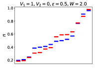
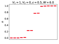
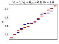
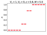
Figure 3: (color online) eigenvalues of the single-particle density matrix (occupation numbers $\{n\}$) corresponding to periodic boundary condition (Blue), and antiperiodic boundary condition (red) for NN interaction of Eq.(2) ($V_{1}=1,V_{2}=0$). In left plots, $\epsilon$ and $W$ are chosen such that we are in the extended phase, while in the right plots, they correspond to the MBL phase. We set $L=14,N=7$. Only one sample is considered, and we do not take disorder average. We see that shifts in the occupation numbers in the MBL phase are almost zero, while the shifts are appreciable in the extended phase.

To have a characterization independent of the system size, we divide $\delta n$ to average level spacing for occupation numbers, $\Delta n$, and introduce the following as an ETH-MBL phase transition characterization:

$$\centering g_{n}=\delta n/\Delta n.\@add@centering$$ (9)

We plot typical averaged $g_{n}$ for the NN case of Eq. (2) ($V_{1}=1,V_{2}=0$) for some selected values of $\epsilon$, as we change disorder strength $W$ in Fig. 4. We see that deep in the delocalized phase, shifts in the eigenvalues of density matrix are on the order of level spacing of the eigenvalues, and it vanishes in the localized phase. At the middle of the spectrum ($\epsilon=0.5$), we obtain $W_{c}\approx 3.6$, consistent with the previously obtained resultsLuitz et al. (2015); Serbyn et al. (2017); Filho et al. (2017); Villalonga et al. (2018). We see that $g_{n}$ is not symmetric about the middle of the spectrum and it is tilted toward smaller $\epsilon$.

Figure 4: (color online) typical averaged $g_{n}=\frac{\delta n}{\Delta n}$ for the NN interaction case of Eq. (2) corresponding to $V_{1}=1,V_{2}=0$, for some selected values of $\epsilon$’s, as we change the disorder strength $W$. We set $L=14,N=7$. We take typical average over altogether $2000$ samples for each data point.

By looking at $g_{n}$, we can locate mobility edges, the points in the energy spectrum, for a fixed value of disorder strength, where phase changes between delocalized and localized . We calculate $g_{n}$ for a fixed value of $W$, as we change $\epsilon$. The results are plotted in Fig. 5. As we can see, there are no mobility edges deep in the localized phase and deep in the delocalized phase, i.e. for $W=1.0$ and $W=4.5$. For $W=1.0$, $g_{n}$ is always non-zero, while for $W=4.5$ it vanishes for all values of $\epsilon$. For other disorder strength values, we can see mobility edges where $g_{n}$ goes to zero. All this information can be summarized in Fig. 6, where $g_{n}$ is calculated for the entire energy spectrum as we change disorder strength $W$(standard deviation of $g_{n}$ is plotted in Fig. 7).

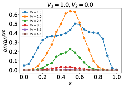
Figure 5: (color online) typical averaged $g_{n}=\frac{\delta n}{\Delta n}$ for the NN interaction case of Eq. (2) corresponding to $V_{1}=1,V_{2}=0$, for some selected values of disorder strength $W$, as energy varies, where we can see the mobility edges. We set $L=14,N=7$. We take typical average over altogether $2000$ samples for each data point.

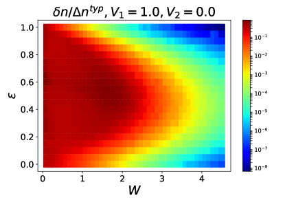
Figure 6: (color online) typical averaged $g_{n}=\frac{\delta n}{\Delta n}$ for the NN interaction case of Eq. (2) corresponding to $V_{1}=1,V_{2}=0$, for the entire energy spectrum as we change the disorder strength $W$. We set $L=14,N=7$. We take typical average over altogether $2000$ samples for each data point.

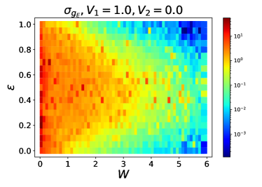
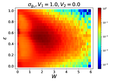
Figure 7: (color online) standard deviation of $g_{E}$ (upper panel) and $g_{n}$ (lower panel) for the entire spectrum of the energy as we change the disorder strength $W$ for the NN interaction case ($V_{1}=1,V_{2}=0$). System size $L=14,N=7$. Number of samples is $2000$ for each data point.

V Nearest-neighbor and next-nearest-neighbor interactions

It is also instructive to apply our method of characterizing ETH-MBL phase transition to the case of having both NN and NNN interactions, corresponds to $V_{1}=1,V_{2}=1$ in Eq. (2). Having NNN interaction in addition to the NN interaction makes localization harder; i.e. we expect that a larger amount of disorder is required to make the state localized at each energy, and thus transition from ETH to MBL phase happens at a larger value of $W_{c}$ compare to the NN case. Obtained results of $g_{E}$ and $g_{n}$ for the case of $V_{1}=1,V_{2}=1$ are plotted in Figs. 8 and 9. As we expected, transition point moves to larger values of disorder strength. We also see that the transition points become more asymmetric compare to the NN case. Moreover, there is no phase transition between ETH and MBL for states with the largest $\epsilon$’s, and those states are localized with a non-zero disorder strength.

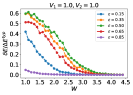
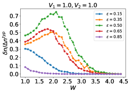
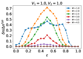
Figure 8: (color online) typical averaged $g_{E}=\frac{\delta E}{\Delta E}$ (left panel) and $g_{n}=\frac{\delta n}{\Delta n}$ (right panel) for the case of having both NN and NNN interactions corresponding to $V_{1}=1,V_{2}=1$ in Eq. (2) for some specific $\epsilon$’s as disorder strength $W$ varies. Right panel: typical averaged $g_{n}=\frac{\delta n}{\Delta n}$ for the case of NN and NNN interactions for some selected values of disorder strength $W$ as energy varies, where we can see the mobility edges. For all plots, We set $L=14,N=7$. We take typical average over altogether $2000$ samples for each data point.

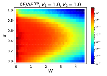
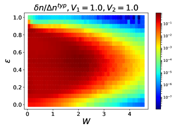
Figure 9: (color online) typical average of $g_{E}=\frac{\delta E}{\Delta E}$ (upper panel) and $g_{n}=\frac{\delta n}{\Delta n}$ (lower panel) for the entire spectrum of the energy as we change the disorder strength $W$ for the case of having both NN and NNN interactions corresponding to $V_{1}=1,V_{2}=1$ in Eq. (2). We set $L=14,N=7$. We take typical average over altogether $2000$ samples for each data point.

VI Conclusion and outlook

Regarding the ETH-MBL phase transition in random interacting systems, finding the phase characterizations are one of main research today. In this work, we introduced new methods for characterizing the phase transition; namely, we studied the response of the system to the boundary conditions. For free fermions, the effect of change in boundary conditions on single-particle eigen-energiesEdwards and Thouless (1972), as well as on the single-particle density matrixPouranvari and Montakhab (2017) has been studied before. Extended eigenstates feel what happens at the boundary, while changes in boundary conditions are not reflected in the localized phase. We extend this idea to the interacting case. In particular, we changed the boundary conditions between periodic and antiperiodic; then, we studied the echo of these changes in the energy of the system and eigenvalues of the single-particle density matrix. We used these characterizations for the case of a 1D model with nearest-neighbor interaction, nearest-neighbor hopping, and disorder which is added by random onsite energies. This model has been studied before, and we know approximately the phase transition point. We could identify the ETH phase with significant shifts in the system’s energy and significant shifts in the occupation numbers (both shifts are on the order of corresponding level spacing). In contrast, the MBL phase has a vanishing response to the change in the boundary conditions. Furthermore, we added extra next-nearest-neighbor interactions and studied its effects on the ETH-MBL phase transition.