ConnectIt: A Framework for Static and Incremental Parallel Graph Connectivity Algorithms

Abstract.

Connected components is a fundamental kernel in graph applications. The fastest existing multicore algorithms for solving graph connectivity are based on some form of edge sampling and/or linking and compressing trees. However, many combinations of these design choices have been left unexplored. In this paper, we design the ConnectIt framework, which provides different sampling strategies as well as various tree linking and compression schemes. ConnectIt enables us to obtain several hundred new variants of connectivity algorithms, most of which extend to computing spanning forest. In addition to static graphs, we also extend ConnectIt to support mixes of insertions and connectivity queries in the concurrent setting.

We present an experimental evaluation of ConnectIt on a 72-core machine, which we believe is the most comprehensive evaluation of parallel connectivity algorithms to date. Compared to a collection of state-of-the-art static multicore algorithms, we obtain an average speedup of 12.4x (2.36x average speedup over the fastest existing implementation for each graph). Using ConnectIt, we are able to compute connectivity on the largest publicly-available graph (with over 3.5 billion vertices and 128 billion edges) in under 10 seconds using a 72-core machine, providing a 3.1x speedup over the fastest existing connectivity result for this graph, in any computational setting. For our incremental algorithms, we show that our algorithms can ingest graph updates at up to several billion edges per second. To guide the user in selecting the best variants in ConnectIt for different situations, we provide a detailed analysis of the different strategies. Finally, we show how the techniques in ConnectIt can be used to speed up two important graph applications: approximate minimum spanning forest and SCAN clustering.

1. Introduction

Computing the connected components (connectivity) of an undirected graph is a fundamental problem for which numerous algorithms have been designed. In the connected components problem, we are given an undirected graph and the goal is to assign labels to the vertices such that two vertices reachable from one another have the same label, and otherwise have different labels (Cormen et al., 2009). A recent paper by Sahu et al. (Sahu et al., 2017) surveying industrial uses of graph algorithms shows that connectivity is the most frequently performed graph computation out of a list of 13 fundamental graph routines including shortest paths, centrality computations, triangle counting, and others. Computing connected components is also used to solve many other graph problems, for example, to solve biconnectivity and higher-order connectivity (Tarjan and Vishkin, 1985), as well as a subroutine in popular clustering algorithms (Ester et al., 1996; Xu et al., 2007; Patwary et al., 2012a; Gan and Tao, 2015; Fang et al., 2016; Wen et al., 2017).

In the sequential setting, connected components can be easily solved using breadth-first search, depth-first search, or union-find. However, it is important to have fast parallel algorithms for the problem in order to achieve high performance. Many parallel algorithms for connected components have been proposed in the literature (see, e.g., (Awerbuch and Shiloach, 1987; Chin et al., 1982; Chong and Lam, 1995; Cole and Vishkin, 1991; Han and Wagner, 1990; Hirschberg et al., 1979; Iwama and Kambayashi, 1994; Johnson and Metaxas, 1997; Karger et al., 1999; Koubek and Krsnakova, 1985; Kruskal et al., 1990; Nath and Maheshwari, 1982; Phillips, 1989; Reif, 1985; Shiloach and Vishkin, 1982; Gazit, 1991; Vishkin, 1984; Shun et al., 2014; Dhulipala et al., 2018; Greiner, 1994; Halperin and Zwick, 1996; Slota et al., 2014; Blelloch et al., 2012; Bader et al., 2005; Bader and JaJa, 1996; Madduri and Bader, 2009; Bader and Cong, 2005; Bus and Tvrdik, 2001; Caceres et al., 2004; Krishnamurthy et al., 1994; Patwary et al., 2012b; Hambrusch and TeWinkel, 1988; Hsu et al., 1997; Nguyen et al., 2013; Hawick et al., 2010; Soman et al., 2010; Banerjee and Kothapalli, 2011; Shun and Blelloch, 2013; Sutton et al., 2018; Jaiganesh and Burtscher, 2018; Liu and Tarjan, 2019; Stergiou et al., 2018; Jain et al., 2017; Kiveris et al., 2014; Iverson et al., 2015; Feng et al., 2018; Cong and Muzio, 2014; Meng et al., 2019; Andoni et al., 2018; Behnezhad et al., 2019b, a, 2020; Zhang et al., 2020; Pai and Pingali, 2016; Ben-Nun et al., 2017; Rastogi et al., 2013; Yan et al., 2014), among many others). Recent state-of-the-art parallel implementations are based on graph traversal (Slota et al., 2014; Dhulipala et al., 2018; Shun et al., 2014; Shun and Blelloch, 2013), label propagation (Slota et al., 2014; Nguyen et al., 2013; Shun and Blelloch, 2013), union-find (Blelloch et al., 2012; Patwary et al., 2012b; Jaiganesh and Burtscher, 2018), or the hook-compress paradigm (Liu and Tarjan, 2019; Shiloach and Vishkin, 1982; Bader et al., 2005; Awerbuch and Shiloach, 1987; Cong and Muzio, 2014; Beamer et al., 2015; Greiner, 1994; Soman et al., 2010; Meng et al., 2019; Wang et al., 2017; Pai and Pingali, 2016; Ben-Nun et al., 2017; Zhang et al., 2020). Recent work by Sutton et al. (Sutton et al., 2018) uses sampling to find the connected components on a subset of the edges, which can be used to reduce the number of edge inspections when running connectivity on the remaining edges. However, most prior work has provided only one, or a few implementations of a specific approach for a particular architecture, and there are many variants of these algorithmic approaches that have been left unexplored.

In this paper, we design the ConnectIt framework for multicore CPUs, which enables many possible implementation choices of the algorithmic paradigms for parallel connectivity from the literature. Furthermore, as many real-world graphs are frequently updated under insertion-heavy workloads (e.g., there are about 6,000 tweets per second on Twitter, but only a few percent of tweets are deleted (Almuhimedi et al., 2013)), ConnectIt provides algorithms that can maintain connectivity under incremental updates (edge insertions) to the graph. A subset of the ConnectIt implementations also support computing the spanning forest of a graph in both the static and incremental settings. We focus on the multicore setting as the largest publicly-available real-world graphs can fit in the memory of a single machine (Dhulipala et al., 2018; Dhulipala et al., 2020b). We also compare ConnectIt’s results with reported results for the distributed-memory setting, showing that our multicore solutions are significantly faster and much more cost-efficient. We have recently extended our techniques to the GPU setting (Hong et al., 2020).

ConnectIt Overview

Algorithms. ConnectIt is designed for min-based connectivity algorithms, which are based on vertices propagating labels to other vertices that they are connected to, and updating labels based on the minimum label received. All of the algorithms conceptually view the label of a vertex $v$ as a directed edge from $v$ to the vertex corresponding to $v$’s label. Thus, these directed edges form a set of directed trees. All of the algorithms that we study maintain acyclicity in this forest (ignoring self-loops at the roots of trees). The min-based algorithms that we study include both root-based algorithms, which include a broad class of union-find algorithms and several other algorithms that only modify the labels of roots of trees in the forest, as well as other min-based algorithms which deviate from this rule and can modify the labels of non-root vertices.

Sampling and Two-phase Execution. Inspired by the Afforest algorithm (Sutton et al., 2018), ConnectIt produces algorithms with two phases: the sampling phase and the finish phase. In the sampling phase, we run connected components on a subset of the edges in the graph, which assigns a temporary label to each vertex. We then find the most frequent label, $L_{\max}$, which corresponds to the ID of the largest component (not necessarily maximal) found so far. In the finish phase, we only need to run connected components on the incident edges of vertices with a label not equal to $L_{\max}$, which can significantly reduce the number of edge traversals. We observe that this optimization is similar in spirit to the direction-optimization in breadth-first search (Beamer et al., 2012), which skips over incoming edges for vertices, once they have already been visited during dense iterations. If sampling is not used, then the finish phase is equivalent to running a min-based algorithms on all vertices and edges.

Our main observation is that these sampling techniques are general strategies that reduce the number of edge traversals in the finish phase, and thus accelerate the overall algorithm. In ConnectIt, any of the min-based algorithms that we consider can be used for the finish phase in combination with any of the three sampling schemes: $k$-out, breadth-first search, and low-diameter decomposition sampling. For the implementations where the finish phase uses a root-based algorithm, ConnectIt also supports spanning forest computation. Our generalized sampling paradigm and integration into ConnectIt enables us to express over 232 combinations of parallel algorithms of parallel graph connectivity and 192 implementations for parallel spanning forest (only our root-based algorithms support spanning forest).

Incremental Connectivity. Due to the frequency of updates to graphs, various parallel streaming algorithms for connected components have been developed (McColl et al., 2013; Ediger et al., 2012; Simsiri et al., 2017; Sengupta and Song, 2017; Acar et al., 2019; Dhulipala et al., 2020a). Motivated by this, the ConnectIt framework supports a combination of edge insertions and connectivity queries in the graph. Both the union-find and root-based algorithm implementations in ConnectIt support batched edge insertions/queries. Additionally, all of the union-find implementations, other than the variants of Rem’s algorithm combined with the splice compression scheme, support asynchronous updates and queries, and most of them are lock-free or wait-free.

System	Graph	Mem. (TB)	Threads	Nodes	Time (s)
Mosaic (Maass et al., 2017)	Hyperlink2014	0.768	1000	1	708
FlashGraph (Zheng et al., 2015)	Hyperlink2012	.512	64	1	461
GBBS (Dhulipala et al., 2018)	Hyperlink2012	1	144	1	25.8
GBBS (NVRAM) (Dhulipala et al., 2020b)	Hyperlink2012	0.376	96	1	36.2
Galois (NVRAM) (Gill et al., 2020)	Hyperlink2012	0.376	96	1	76.0
Slota et al. (Slota et al., 2016)	Hyperlink2012	16.3	8192	256	63
Stergiou et al. (Stergiou et al., 2018)	Hyperlink2012	128	24000	1000	341
Gluon (Dathathri et al., 2018)	Hyperlink2012	24	69632	256	75.3
Zhang et al. (Zhang et al., 2020)	Hyperlink2012	$\geq 256$	262,000	4096	30
ConnectIt	Hyperlink2014	1	144	1	2.83
	Hyperlink2012	1	144	1	8.20

Table 1. System configurations, including memory (terabytes), num. hyper-threads and nodes, and running times (seconds) of connectivity results on the Hyperlink graphs. The last rows show the fastest ConnectIt times. The fastest time per graph is shown in green.

Experimental Evaluation. We conduct a comprehensive experimental evaluation of all of the connectivity and spanning forest implementations in ConnectIt on a 72-core multicore machine, in both the static and incremental setting. Compared to existing work, the ConnectIt implementations significantly outperform state-of-the-art implementations using the new sampling techniques proposed in this paper, and often outperform prior work even without applying sampling. Our fastest algorithms using sampling are always faster than the fastest currently available implementation. As an example of our high performance, ConnectIt is able to produce implementations that can process the Hyperlink2012 graph (Meusel et al., 2015), which is the largest publicly-available real-world graph and has over 3.5 billion vertices and 225 billion directed edges, on a single 72-core machine with a terabyte of RAM. We show existing results on this graph, and the smaller Hyperlink2014 graph (1.7 billion vertices and 128 billion directed edges) in Table 1. Our running times are between 3.65–41.5x faster than existing distributed-memory results that report results for Hyperlink2012, while using orders of magnitude fewer computing resources. Finally, we show that ConnectIt can be used to speed up two graph applications: approximate minimum spanning forest and index-based SCAN clustering.

Contributions. The contributions of this paper are as follows.

1. We introduce ConnectIt, which provides several hundred different multicore implementations of connectivity, spanning forest, and incremental connectivity, most of which are new.

2. ConnectIt provides different choices of sampling methods based on provably-efficient graph algorithms, which can be used in two-phase execution to reduce the number of edge traversals.

3. The fastest implementation in ConnectIt achieves an average speedup of 2.3x (and ranges from 1.5–4.02x speedup) over the fastest existing static multicore connectivity algorithms.

4. For incremental connectivity, the multicore implementations in ConnectIt achieve a speedup of 1,461–28,364x over existing multicore solutions and a throughput (in terms of directed edges) of between 4.6 million insertions per second for very small batch sizes to 7.1 billion insertions per second for large batches, on graphs of varying sizes.

5. We present a detailed experimental analysis of the different implementations in ConnectIt to guide the user into finding the most efficient implementation for each situation.

6. We show that ConnectIt can be used to speed up approximate minimum spanning forest by 2.03–5.36x and index-based SCAN clustering by 42.5–50.5x.

7. The ConnectIt source code is available at https://github.com/ParAlg/gbbs/tree/master/benchmarks/Connectivity/ConnectIt.

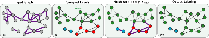
Figure 1. This figure illustrates the ConnectIt framework for connectivity using $k$-out Sampling on a small input graph. (i) illustrates the input graph. The bolded purple edges are those selected by the $k$-out sample with $k=2$. (ii) shows the partial connectivity labeling after computing connectivity on the sampled edges (e.g., using a union-find algorithm). $L_{\max}$ indicates the vertices in the largest component (shown in green). (iii) shows the edges (bolded in purple) which still must be processed in the finish step, namely all edges incident to vertices $v\notin L_{\max}{}$. Lastly, (iv) shows the output connectivity labeling.

2. Preliminaries

Graph Notation and Formats. We denote an unweighted graph by $G(V,E)$, where $V$ is the set of vertices and $E$ is the set of edges in the graph. We use $n=|V|$ to refer to the number of vertices and $m=|E|$ to refer to the number of directed edges. In our graph representations, vertices are indexed from $0$ to $n-1$, and we consider two graph formats—compressed sparse row (CSR) and edge/coordinate list (COO). In CSR, we are given two arrays, $I$ and $A$, where the incident edges of a vertex $v$ are stored in $\{A[I[v]],\ldots,A[I[v+1]-1]\}$ (we assume $A[n]=m$). In COO, we are given an array of pairs $(u,v)$ corresponding to edge endpoints. Unless otherwise mentioned, we store graphs in the CSR

Compare-and-Swap. A compare-and-swap (CAS) takes three arguments: a memory location x, an old value oldV, and a new value newV. If the value stored at x is equal to oldV, the CAS atomically updates the value at x to be newV and returns true; otherwise the CAS returns false. CAS is supported by most modern processors.

Work-Depth Model. We analyze our parallel algorithms using the work-depth measure (Jaja, 1992; Cormen et al., 2009). The work is the number of operations used by the algorithm and the depth is the length of the longest sequential dependence. The work-depth measure is a fundamental tool in analyzing parallel algorithms, e.g., see  (Blelloch et al., 2016; Dhulipala et al., 2018; Gu et al., 2015; Shun et al., 2014; Sun et al., 2019, 2018; Wang et al., 2020; Dhulipala et al., 2020b) for a sample of recent practical uses of this model.

Linearizability. Linearizability (Herlihy and Wing, 1990; Herlihy and Shavit, 2012) is the standard correctness criteria for concurrent algorithms. A set of operations are linearizable if the result of a concurrent execution is the same as if the operations were applied at a distinct point in time (the linearization point) between the operation’s invocation and response. The sequential ordering of the operations based on their linearization points is its linearization order.

Graph Connectivity and Related Problems. A connected component (CC) in $G$ is a maximal set of vertices, such that there is a path between any two vertices in the set. An algorithm for computing connected components returns a connectivity labeling $C$ for each vertex, such that $C{}(u)=C{}(v)$ if and only if vertices $u$ and $v$ are in the same connected component. We represent connectivity labelings using an array of $n$ integers. A partial connectivity labeling is a labeling $C{}$ such that $C{}(u)=C{}(v)$ implies that $u$ and $v$ are in the same component. A connectivity query takes as input two vertex identifiers and returns true if and only if their labels are the same. A spanning forest (SF) in $G=(V,E)$ contains one tree for each connected component in $G$ containing all vertices of that component. A breadth-first search (BFS) algorithm takes as input a graph $G=(V,E)$ and a source vertex $\mathit{src}\in V$, and traverses the vertices reachable from $\mathit{src}$ in increasing order of their distance from $\mathit{src}$. A low-diameter decomposition (LDD) of a graph parameterized by $0<\beta<1$ and $d$ is a partition of the vertices into $V_{1},\ldots,V_{k}$, such that the shortest path between any two vertices in the same partition using only intra-partition edges is at most $d$, and the number of inter-partition edges is at most $\beta m$ (Miller et al., 2013).

A union-find (or disjoint-set) data structure maintains a collection of sets where all elements in each set are associated with the same label. The data structure is represented as a forest where each element has a parent pointer (with the root of each tree pointing to itself), and the label of an element is the root of the tree it belongs to. A union-find data structure supports the MakeSet, Union, and Find operations (Cormen et al., 2009). MakeSet($e$) creates a new set containing just the element $e$ with a parent pointer to itself. Union($e$,$e^{\prime}$) merges together the trees of $e$ and $e^{\prime}$ into a single tree, if they are not already in the same tree. Find($e$) returns the label of element $e$ by looking up the root of the tree that $e$ belongs to. The Find and Union operations can compress paths in the tree to speed up future operations. When used in a CC algorithm, the elements are vertices, and at the end of the algorithm, Find($v$) returns $C{}(v)$. There are various versions of union-find based on how the Union and Find operations are implemented, and this paper explores a large number of union-find implementations for the concurrent setting.

A min-based connectivity algorithm also maintains a set data structure, like union-find algorithms. A min-based algorithm only updates the label of an element if the new label is smaller than the previous one. All of the connectivity algorithms studied in this paper are min-based algorithms. A root-based connectivity algorithm is a special type of min-based algorithm. Specifically, a root-based algorithm only links sets together by adding a link from the root of one tree, to a node in another tree.

3. ConnectIt Framework

In this section, we define the components of the ConnectIt framework and the specific ways in which they can be combined. We start by presenting our algorithm for computing connectivity. The algorithm supports combining multiple sampling methods and finish methods, which we describe in detail in Sections 3.2 and 3.3. Figure 1 illustrates how the ConnectIt framework works for a $k$-out sampling algorithm on an example graph.

Next, in Sections 3.4 and 3.5, we describe modifications required to adapt our framework for spanning forest, and for the incremental setting. We present correctness proofs for our algorithms in all of the settings in Appendix B. Finally, in Section 3.6 we describe details regarding our implementation.

3.1. Connectivity

Algorithm 1 ConnectIt Framework: Connectivity

1:procedure Connectivity($G(V,E),\mathit{sample\_f},\mathit{finish\_f}$)

2:    $\mathit{sampling}\leftarrow\textsc{GetSamplingAlgorithm}(\mathit{sample\_opt})$

3:    $\mathit{finish}\leftarrow\textsc{GetFinishAlgorithm}(\mathit{finish\_opt})$

4:    $\mathit{labels}\leftarrow\{i\rightarrow i\ |\ i\in[|V|]\}$

5:    $\mathit{labels}\leftarrow\mathit{sampling}.\textsc{SampleComponents}(G,\mathit{labels})$

6:    $L_{\max}{}\leftarrow\textsc{IdentifyFrequent}(\mathit{labels})$

7:    $\mathit{labels}\leftarrow\mathit{finish}.\textsc{FinishComponents}(G,\mathit{labels},L_{\max}{})$

8:    return$\ \mathit{labels}$

A connectivity algorithm in ConnectIt is instantiated by supplying $\mathit{sampling}$ and $\mathit{finish}$ methods. Algorithm 1 presents the generic ConnectIt connectivity algorithm, parameterized by these user-defined functions. The algorithm first initializes a connectivity labeling, which is represented as an array of $n$ integers, by setting each vertex’s label to be its own ID (Line 4). It then performs a sampling step using the provided $\mathit{sampling}$ algorithm (Line 5). The sampling step results in partial connectivity information being computed and stored in the $\mathit{labels}$ array. Next, it identifies $\bm{L_{\max}{}}$, the most frequently occurring component ID in the $\mathit{labels}$ array (Line 6). The identified component is then supplied to the $\mathit{finish}$ algorithm, which finishes computing the connected components of $G$. The finish method potentially saves significant work by avoiding processing vertices in the component with an ID of $L_{\max}{}$.

Properties of Sampling Methods. Before discussing the sampling and finish methods, we discuss the properties that we require in ConnectIt to obtain a correct parallel connectivity algorithm.

Definition 3.0.

Consider a graph $G$. Let $C{}$ be the labeling produced by a sampling method $S$ and let the labeling $C{}^{\prime}=\textsc{Connectivity}$ $(G[C{}])$ where $G[C{}]$ is the graph induced by contracting $G$ using $C{}$. We say that a sampling method $S$ is correct if:

$C{}^{\prime\prime}=\{C{}^{\prime}[C{}[v]]\ |\ v\in V\}$ is a correct connectivity labeling.

In other words the definition states that the connectivity label found by composing the sampled label $(C{}[v])$ with the connectivity label of the contracted vertex on the contracted graph, i.e., $C{}^{\prime}[C{}[v]]$, yields a correct connectivity labeling.

Properties of Finish Methods. Next, we define the correctness properties for finish methods in ConnectIt. The definition uses the interpretation of labels as rooted trees, which we discussed above.

Definition 3.0.

Let $C{}$ be a connectivity labeling, which initially maps every vertex to its own node ID. We call a connectivity algorithm monotone if the algorithm updates the labels such that the updated labeling can be represented as the union of two trees in the previous labeling.

In other words, once a vertex is connected to its parent in a tree, it will always be in the same tree as its parent. Finally, we define linearizable monotonicity, which is the relaxed correctness property possessed by most finish algorithms in our framework.

Definition 3.0.

Given an undirected graph $G(V,E)$, we say that a connectivity algorithm operating on a connectivity labeling $C{}$ is linearizably monotone if

1. Its operations are linearizable.

2. Every operation in the linearization preserves monotonicity.

The finish methods considered in ConnectIt are linearizably monotone, with only a few exceptions. The first is a subset of the variants of Rem’s algorithms (all variants using the splice rule), which we analyze separately (Theorem 3), and the family of other min-based connectivity algorithms, which includes a subset of Liu-Tarjan algorithms, Stergiou’s algorithm, Shiloach-Vishkin, and label propagation (Theorem 5).

3.2. Sampling Algorithms

This section introduces the correct sampling methods used in ConnectIt. We provide pseudocode for our sampling methods in Appendix D.1.

$k$-out Sampling. The $k$-out method takes a positive integer parameter $k$, selects $k$ edges out of each vertex uniformly at random, and computes the connected components of this sampled graph. An important result shown in a recent paper by Holm et al. (Holm et al., 2019) is that if $nk$ edges are sampled in this way for sufficiently large $k$, only $O(n/k)$ inter-component edges remain after contraction, in expectation. Holm et al. conjecture that this fact about the number of inter-component edges holds for any $k\geq 2$, although the proof holds for $k=\Omega(\log n)$. Sutton et al. (Sutton et al., 2018) describe a sampling scheme that selects the first $k$ edges incident to the vertex, which does not use randomization. However, on some graphs with poor orderings, this method can result in only a small fraction of the components being discovered (leaving up to several orders of magnitude more inter-component edges), which results in a costly sampling step that provides little benefit. To improve our results for these poorly ordered graphs while achieving good performance on graphs where this heuristic performs well, we select the first edge incident to each vertex, and select the remaining $k-1$ edges randomly. To the best of our knowledge, using randomness in this experimental setting has not been explored before. We provide a full evaluation of different options in Appendix C.5.

Breadth-First Search Sampling. The breadth-first search (BFS) sampling method is a simple heuristic based on using a breadth-first search from a randomly chosen source vertex. Assuming that the graph contains a massive component, containing, say, at least a constant fraction of the vertices, running a BFS from a randomly selected vertex will discover this component with constant probability. To handle the case where we are unlucky and pick a bad vertex, we can apply this process $c$ times. Setting $c=\Theta(\log n)$ would ensure that we find the massive component with high probability. In practice we set $c=3$, and in our experiments we found that one try was sufficient to discover the massive component on all of the real-world graphs we test on. ConnectIt terminates the sampling algorithm when a component containing more than 10% of the vertices is found or after $c$ rounds, whichever happens first.

Low-Diameter Decomposition Sampling. As discussed in Section 2, running an LDD algorithm on a graph with parameter $\beta<1$ partitions the graph into clusters such that the strong diameter (the shortest path using only edges inside the cluster) of each cluster is $O(\log n/\beta)$, and cuts $O(\beta m)$ edges in expectation (Miller et al., 2013). Shun et al. (Shun et al., 2014) give a simple and practical work-efficient (linear-work) parallel connectivity algorithm based on recursively applying LDD and performing graph contraction to recurse on a contracted graph.

In this paper, we consider applying just a single round of the LDD algorithm of Miller, Peng, and Xu (Miller et al., 2013), without actually contracting the graph after performing the LDD. On low-diameter graphs, the hope is that much of the largest connected component will be contained in the most frequent cluster identified. Our approach is practically motivated by studying the behavior of the work-efficient connectivity algorithm of Shun et al. (Shun et al., 2014) on low-diameter real-world graphs and observing that after one application of LDD, the resulting clustering contains a single massive cluster, and the number of distinct clusters in the contracted graph is extremely small. We provide an empirical analysis of this sampling method for different values of $\beta$ in Appendix C.5

In Appendix B.1, we prove that $k$-out Sampling, BFS Sampling, and LDD Sampling are all correct, i.e., they all produce connectivity labeling satisfying Definition 1.

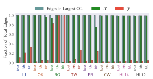
Figure 2. Bar plot showing the performance of different sampling strategies on eight large real-world graphs in terms of the number of edges in the largest connected component, the number of edges in the most frequent sampled component ($\mathcal{X}$) and the number of edges processed by the sampling strategy ($\mathcal{Y}$). All quantities are shown as a fraction of the total number of edges, $m$.

The Potential Benefits of Sampling. Intuitively, the main advantage of our sampling schemes is that if the graph has a single large component containing a significant fraction of the edges, applying a sampling method can allow us to skip processing most of these edges. Specifically, suppose applying a correct sampling scheme uncovers a frequent component $L_{\max}$ containing $\mathcal{X}$ edges while processing only $\mathcal{Y}$ edges. Then, by skipping processing vertices in $L_{\max}$ in the finish phase, the total number of edges that are processed by the algorithm is $m-\mathcal{X}+\mathcal{Y}$.

Figure 2 illustrates the potential benefits from applying our sampling schemes on a suite of large real-world graphs (see Section 4 for graph details). We observe that $\mathcal{X}$ is usually a large fraction of both the number of edges in the largest component and of $m$, indicating that the sampling methods can help us skip nearly all of the edges in the graph in the finish phase. The one exception is the road_usa (RO) graph, where LDD and BFS Sampling both suffer due to the graph’s large diameter, which we discuss in more detail in Section 4.1. However, both LDD and BFS Sampling perform well on the other low-diameter graphs since direction-optimization enables them to complete while only examining a small number of edges. Note that applying LDD on high-diameter graphs results in a large number of small clusters, and thus this scheme is better suited for low-diameter graphs (Miller et al., 2013). We observe that $k$-out Sampling results in a large value of $\mathcal{X}$ in all cases. Finally, $\mathcal{Y}$ is typically significantly smaller than $\mathcal{X}$ indicating that our approach enables us to process $\mathcal{Y}+(m-\mathcal{X})$ edges in total, which is only a small fraction of $m$.

3.3. Finish Algorithms

We now describe different min-based methods that can be used as finish methods in our framework. All of the finish methods that we describe can be combined with any of the sampling methods described in Section 3.2. We provide implementations of several different algorithm classes, which internally have many options that can be combined to generate different instantiations of the algorithm. The min-based algorithms that we consider as part of the framework are union-find (many different variants, described below), Shiloach-Vishkin (Shiloach and Vishkin, 1982), Liu-Tarjan (Liu and Tarjan, 2019), Stergiou (Stergiou et al., 2018), and label propagation. An important feature of ConnectIt is in modifying these finish methods to avoid traversing the vertices with the most frequently occurring ID as identified from sampling in Algorithm 1. We provide pseudocode for all of our implementations described in this section in Appendix B.

3.3.1. Union-Find

We consider several different concurrent (asynchronous) union-find algorithms, which are all min-based. All of these algorithms are linearizably monotone for a set of concurrent union and find operations, with the exception of the concurrent Rem’s algorithm variants using the splice rule, which are linearizable only for a set of concurrent union operations or a set of concurrent find operations, but not for mixed operations. All of these algorithms can be combined with sampling by simply skipping traversing the vertices with label equal to $L_{\max}{}$ after sampling.

Asynchronous Union-Find. The first class of algorithms are inspired by a recent paper exploring concurrent union-find implementations by Jayanti and Tarjan (Jayanti and Tarjan, 2016). We implement all of the variants from their paper, as well as a full path compression technique (also considered in (Alistarh et al., 2019)) which works better in practice in some cases. We refer to this union-find algorithm as $\bm{\mathsf{UF\mathchar 45\relax Async}{}}$ since it is the classic union-find algorithm directly adapted for an asynchronous shared-memory setting. The algorithm links from lower-indexed to higher-indexed vertices to avoid cycles, and only performs links on roots (thus implying that the algorithm is monotone). This algorithm can be combined with the following implementations of the find operation: $\bm{\mathsf{FindNaive}}$, which performs no compression during the operation; $\bm{\mathsf{FindSplit}}$ and $\bm{\mathsf{FindHalve}}$, which perform path-splitting and path-halving, respectively; and $\bm{\mathsf{FindCompress}}$, which fully compresses the find path. Jayanti and Tarjan show that this class of algorithms is linearizable for a set of concurrent union and find operations (they do not consider $\mathsf{FindCompress}$, but it is relatively easy to show that it is linearizable). The fact that these algorithms are linearizably monotone for a set of concurrent union and find operations follows from the observation that they only link roots, and thus all label changes made by the operations are the result of taking the union of trees.

We also consider two similar variants of the $\mathsf{UF\mathchar 45\relax Async}$ algorithm: $\mathsf{UF\mathchar 45\relax Hooks}$ and $\mathsf{UF\mathchar 45\relax Early}$. $\bm{\mathsf{UF\mathchar 45\relax Hooks}{}}$ is closely related to $\mathsf{UF\mathchar 45\relax Async}$, with the only difference between the algorithms being that instead of performing a CAS directly on the array storing the connectivity labeling, we perform a CAS on an auxiliary $\mathit{hooks}$ array, and perform an uncontended write on the $\mathit{parents}$ array. $\bm{\mathsf{UF\mathchar 45\relax Early}{}}$ is also similar to $\mathsf{UF\mathchar 45\relax Async}$, except that the algorithm traverses the paths from both vertices together, and tries to eagerly check and hook a vertex once it is a root. The algorithm can optionally perform a find on the endpoints of the edge after the union operation finishes, which has the effect of compressing the find path. The linearizability proof for $\mathsf{UF\mathchar 45\relax Async}$ by Jayanti and Tarjan (Jayanti and Tarjan, 2016) applies to $\mathsf{UF\mathchar 45\relax Hooks}$ and $\mathsf{UF\mathchar 45\relax Early}$, and shows that both algorithms are linearizable for a set of concurrent find and union operations. Thus, these algorithms are also linearizably monotone for a set of concurrent union and find operations as they only link roots.

Randomized Two-Try Splitting. Next, we incorporate a more sophisticated randomized algorithm by Jayanti, Tarjan, and Boix-Adserà (Jayanti et al., 2019), and refer to this algorithm as $\bm{\mathsf{UF\mathchar 45\relax JTB}{}}$. The algorithm either performs finds naively, without using any path compression ($\bm{\mathsf{FindNaive}{}}$), or uses a strategy called $\bm{\mathsf{FindTwoTrySplit}}$, which guarantees provably-efficient bounds for their algorithm, assuming a source of random bits. We refer to (Jayanti et al., 2019) for the pseudocode and proofs of correctness. In particular, they show that the algorithm has low total expected work, and low cost per operation with high probability. Since the $\mathsf{UF\mathchar 45\relax JTB}$ algorithm is linearizable, and only links roots, the algorithm is also linearizably monotone. Extending Theorem 4.1 in (Jayanti et al., 2019) to the work-depth setting, we have the following corollary:

Corollary 0.

The $\mathsf{UF\mathchar 45\relax JTB}$ algorithm solves connectivity in $O(m\cdot(\alpha(n,m/(np))+\log(1+np/m)))$ expected work and $O(\log n)$ depth with high probability.

Concurrent Rem’s Algorithm. We implement two concurrent versions of Rem’s algorithm (Rem’s algorithm was first published in Dijkstra’s book (Dijkstra, 1976)): a lock-based version by Patwary et al. (Patwary et al., 2012b) ($\bm{\mathsf{UF\mathchar 45\relax Rem\mathchar 45\relax Lock}{}}$) and a lock-free compare-and-swap based implementation ($\bm{\mathsf{UF\mathchar 45\relax Rem\mathchar 45\relax CAS}{}}$). Our implementations of Rem’s algorithm can be combined with the same rules for path compression described for $\mathsf{Union}$ above, with one exception which we discuss below. In addition to path compression strategies, our implementations of Rem’s algorithm take an extra splice strategy, which is used when a step of the union algorithm operates at a non-root vertex. Specifically, our algorithms support the $\bm{\mathsf{HalveAtomicOne}{}}$, $\bm{\mathsf{SplitAtomicOne}{}}$, and $\bm{\mathsf{SpliceAtomic}{}}$ rules. The first two rules perform a single path-halving or path-splitting. The third rule performs the splicing operation described in Rem’s algorithm, which atomically swaps the parent of the higher index vertex in the path to the lower index vertex. Combining the $\mathsf{FindCompress}$ option with the $\mathsf{SpliceAtomic}$ rule results in an incorrect algorithm, and so we exclude this single combination. All variants of Rem’s algorithm that do not perform $\mathsf{SpliceAtomic}{}$ are linearizable for a set of concurrent union and find operations by simply following the proof of Jayanti and Tarjan (Jayanti and Tarjan, 2016). The implementations of Rem’s algorithm combined with $\mathsf{SpliceAtomic}$ do not satisfy linearizability of both concurrent find and union operations. In Appendix B.2.2 (Theorem 3), we show that the algorithm is correct in the phase-concurrent setting, where union and find operations are separated by a barrier.

We note that a recent paper by Alistarh et al. (Alistarh et al., 2019) performed a careful performance evaluation of concurrent union-find implementations for multicores on much smaller graphs. They introduce a lock-free version of concurrent Rem’s algorithm with path-splitting similar to our implementation, but do not prove that the algorithm is correct, or consider other path-compaction methods in their algorithm. Compared to their lock-free Rem’s implementation, our implementation is more general, allowing the algorithm to be combined with path-halving and splicing in addition to path-splitting.

3.3.2. Other Min-Based Algorithms

Lastly, we overview the other min-based algorithms supported by ConnectIt.

Liu-Tarjan’s Algorithms. Recently, Liu and Tarjan present a framework for simple concurrent connectivity algorithms based on several rules that manipulate an array of parent pointers using edges to transmit the connectivity information (Liu and Tarjan, 2019). These algorithms are not true concurrent algorithms, but really parallel algorithms designed for the synchronous Massively Parallel Computation ($\mathsf{MPC}$) setting. We implement the framework proposed in their paper as part of ConnectIt. Their framework ensures that the parent array is a minimum labeling, where each vertex’s parent is the minimum value among candidates that it has observed.

Conceptually, each round of an algorithm in the framework processes all remaining edges and performs several rules on each edge. On each round, each vertex observes a number of candidates and updates its parent at the end of the round to the minimum of its current parent, and all candidates. Each round performs a connect phase, a shortcut phase, and possibly an alter phase. The connect phase updates the parents of edges based on different operations, the shortcut phase performs path compression, and the optional alter phase updates the endpoints of an edge to be the current labels of its endpoints. We provide details of the different options for implementing each phase in Appendix D.

Liu and Tarjan prove that all of the algorithm combinations generated from their framework are correct, but only analyze five particular algorithms in terms of their parallel round complexity. In addition to the five original algorithms considered by Liu and Tarjan, we consider a number of algorithm combinations that were not explored in the original paper. We evaluate all algorithm combinations that are expressible in the Liu-Tarjan framework, which we list in Appendix D. Note that only the root-based algorithms in the Liu-Tarjan framework are linearizably monotone. The remaining algorithms are not monotone since a non-root vertex can be moved to a different subtree (one where the previous tree and new trees are disconnected). The non-monotone algorithms result in correct connectivity algorithms due to the fact that edges which were previously applied continue to be applied in subsequent rounds of the algorithm (Liu and Tarjan, 2019).

Stergiou et al.’s Algorithm. Stergiou et al. (Stergiou et al., 2018) recently proposed a min-based connectivity algorithm for the massively parallel computation setting, which is not monotone. We implement the algorithm as part of the Liu-Tarjan framework, within which it can be viewed as a particular instantiation of the Liu-Tarjan rules (Liu and Tarjan, 2019).

Shiloach-Vishkin and Label Propagation. ConnectIt also includes the classic Shiloach-Vishkin ($\mathsf{SV}$) algorithm, which is linearizably monotone, and the folklore label propagation ($\mathsf{Label\mathchar 45\relax Prop}$) algorithm, which is not monotone, both of which we discuss in Appendix B.2.4.

Sampling for Other Min-Based Algorithms. Lastly, we describe how to combine the other min-based algorithms above which are not monotone with the sampling algorithms in ConnectIt. If the largest component after sampling, which has ID $L_{\max}{}$, is relabeled such that all vertices in this component have the smallest possible ID, then these vertices will never change components, and we thus we never have to inspect edges oriented out of these vertices. We show that this modification produces correct algorithms by viewing the largest component as a single contracted vertex that only preserves its inter-cluster edges, and then applying the correctness proof for a connectivity algorithm in the Liu-Tarjan framework (Liu and Tarjan, 2019). We provide a detailed proof in Theorem 5 in the Appendix B.

3.4. Spanning Forest

We also extend ConnectIt to generate a spanning forest of the graph. We show that the class of root-based algorithms can be converted in a black-box manner from parallel connectivity algorithms to parallel spanning forest algorithms. This class consists of every finish algorithm discussed in Section 3.3, with the exception of the Liu-Tarjan algorithms that are not root-based, and Stergiou’s algorithm. We defer our description to Appendix B.3.

3.5. Streaming

We now discuss how ConnectIt supports streaming graph connectivity in the parallel batch-incremental and wait-free asynchronous settings. Formally, an algorithm in the parallel batch-incremental streaming setting receives a sequence of batches of operations, where each batch consists of Insert$(u,v)$ operations and IsConnected$(u,v)$ queries. The algorithm must process the batches one after the other, but operations within a batch are not ordered, and so the streaming algorithm can use parallelism to accelerate processing a batch. We also consider the stronger asynchronous setting. Formally, in the wait-free asynchronous streaming setting, operations are not presented to the algorithm as batches, but instead the Insert and IsConnected operations can be called concurrently by a set of asynchronous threads (Herlihy and Shavit, 2012). Note that any wait-free asynchronous algorithm can be easily extended to a parallel batch-incremental algorithm by simply invoking the concurrent implementation on every operation in parallel. ConnectIt supports the following types of algorithms in the streaming setting:

1. The union-find algorithms in Section 3.3.1, excluding Rem’s algorithms with the $\mathsf{SpliceAtomic}$ method. These algorithms are linearizably monotone in both the parallel batch-incremental and wait-free asynchronous settings.

2. Shiloach-Vishkin ($\mathsf{SV}$) and the root-based $\mathsf{Liu\mathchar 45\relax Tarjan}$ algorithms. These algorithms are linearizably monotone in the parallel batch-incremental setting, although we show that IsConnected queries can be applied concurrently in the wait-free asynchronous setting. However, in these algorithms insertions cause edges to be processed multiple times until convergence, so they must be processed in batches.

3. $\mathsf{UF\mathchar 45\relax Rem\mathchar 45\relax CAS}$ and $\mathsf{UF\mathchar 45\relax Rem\mathchar 45\relax Lock}$ using $\mathsf{SpliceAtomic}$. For this class of algorithms, we consider the phase-concurrent setting which lies between the wait-free asynchronous and parallel batch-incremental settings. Essentially, in this setting, we have a synchronous barrier between insertion and query phases, but within a phase, operations can be called concurrently, like in the wait-free asynchronous setting.

Due to space constraints, we provide details about our streaming algorithm in ConnectIt in Appendix B.

3.6. Implementation

Our implementation of ConnectIt is written in C++, and uses template specialization to generate high-performance implementations while ensuring that the framework code is high-level and general. Using ConnectIt, we can instantiate any of the supported connectivity algorithm combinations using one line of code. Implementing a new sampling algorithm is done by creating a new structure that implements the sampling method for connectivity (and if applicable, a specialized implementation for spanning forest). The sampling code emits an array containing the partial connectivity information. Additionally, for spanning forest the code emits a subset of the spanning forest edges corresponding to the partial connectivity information. Implementing a new finish algorithm is done by implementing a structure providing a FinishComponents method. If the finish algorithm supports spanning forest, it also implements a FinishForest method. Finally, if it supports streaming, the structure implements a ProcessBatch method, taking a batch of updates, and returning results for the queries in the batch. We note that our code can be easily extended to the wait-free asynchronous setting.

We use the compression techniques provided by Ligra+ (Shun et al., 2015; Dhulipala et al., 2018) to process the large graphs used in our experiments. Storing the largest graph used in our experiments in the uncompressed format would require well over 900GB of space to store the edges alone. However, the graph requires only 330GB when encoded using byte codes. The compression scheme uses difference-encoding for each vertex’s adjacency list, storing the differences using variable-length byte codes. This compression scheme is supported by the Graph Based Benchmark Suite (GBBS) (Dhulipala et al., 2018; Dhulipala et al., 2020c), and we used this code base as the basis for implementing ConnectIt.

4. Evaluation

Overview. We show the following results in this section:

• Without sampling, the $\mathsf{UF\mathchar 45\relax Rem\mathchar 45\relax CAS}$ algorithm using the options $\{\mathsf{SplitAtomicOne}{},\mathsf{HalveAtomicOne}{}\}$ is the fastest ConnectIt algorithm across all graphs (Section 4.1).

• Performance analysis of the union-find variants (Section 4.1.1).

• With sampling, the $\mathsf{UF\mathchar 45\relax Rem\mathchar 45\relax CAS}$ algorithm using the options $\{\mathsf{SplitAtomicOne}{},\mathsf{HalveAtomicOne}{}\}$ is consistently the fastest algorithm in ConnectIt (Section 4.2).

• The fastest ConnectIt algorithms using sampling significantly outperform existing state-of-the-art results (Section 4.3).

• ConnectIt streaming algorithms achieve throughputs between 108M–7.16B directed edge insertions per second across all inputs. Our algorithms achieve high throughput even at small batch sizes, and have consistent latency (Section 4.4).

• ConnectIt’s streaming algorithms outperform the streaming algorithm from STINGER, an existing state-of-the-art graph streaming system, by between 1,461–28,364x (Section 4.4).

• An evaluation of ConnectIt’s fastest algorithms on synthetic networks, and guidelines for selecting sampling and finish methods based on graph propertries (Section 4.5).

We show the additional experimental results in the appendix:

• An analysis of the three sampling schemes considered in this paper, showing how these schemes behave in practice as a function of their parameters, and different implementation choices. One of our main observations is that in practice, the number of inter-cluster edges left after $k$-out Sampling is significantly less than $n/k$ (Appendix C.5).

• The fastest ConnectIt algorithms with sampling are as fast as or faster than basic graph routines that perform one indirect read per edge.

• We compare ConnectIt’s performance on very large graphs (Table 1), to the performance of state-of-the-art external-memory, distributed-memory, and shared-memory systems.

• The trends for spanning forest are similar to connectivity, and on average the additional overhead needed to obtain the spanning forest compared to connectivity is 23.7%.

Graph	$n$	$m$	Diam.	Num C.	Largest C.	LT-DC (s)	LT (s)
RO	23.9M	57.7M	6,809	1	23.9M	0.108	0.241
LJ	4.8M	85.7M	16	1,876	4.8M	0.101	0.226
CO	3.1M	234.4M	9	1	3.1M	0.094	0.520
TW	41.7M	2.4B	23*	1	41.7M	0.115	2.80
FR	65.6M	3.6B	32	1	65.6M	0.182	6.07
CW	978.4M	74.7B	132*	23.7M	950.5M	0.534	54.2
HL14	1.7B	124.1B	207*	129M	1.57B	1.02	101.3
HL12	3.6B	225.8B	331*	144M	3.35B	1.64	192.5

Table 2. Graph inputs, including vertices, directed edges, graph diameter, the number of components (Num C.), the number of vertices in the largest component (Largest C.), and the time required in seconds to load the graph input in the binary CSR format used in GBBS, assuming that the graph is already in the disk-cache (LT-DC). The loading time (LT) is the time to fully read the input graph from a 1TB Samsung-SM961 SSD. (The focus of this paper is not on accelerating this hardware-dependent loading time, but on accelerating connected components in the in-memory setting where the data is already in the disk-cache.) We mark diameter values where we are unable to calculate the exact diameter with * and report the effective diameter observed during our experiments, which is a lower bound on the actual diameter.

Experimental Setup. Our experiments are performed on a 72-core Dell PowerEdge R930 (with two-way hyper-threading) with $4\times 2.4\mbox{GHz}$ Intel 18-core E7-8867 v4 Xeon processors (with a 4800MHz bus and 45MB L3 cache) and 1TB of main memory. Our programs use a work-stealing scheduler that we implemented. The scheduler is implemented similarly to Cilk for parallelism (Blelloch et al., 2020). Our programs are compiled with the g++ compiler (version 7.3.0) with the -O3 flag. We use the command numactl -i all to balance the memory allocations across the sockets. All of the numbers we report are based on our parallel implementations on 72 cores with hyper-threading.

Graph Data. To show how ConnectIt performs on graphs at different scales, we selected a representative set of real-world graphs of varying sizes. Most of our graphs are Web graphs and social networks—low-diameter graphs that are frequently used in practice. To test our algorithms on high-diameter graphs, we also ran our implementations on a road network.

Table 2 lists the graphs we use. We used a collection of graphs at different scales, including the largest publicly-available graphs. road_usa (RO) is an undirected road network from the DIMACS challenge (Demetrescu et al., 2019). LiveJournal (LJ) is a directed graph of the LiveJournal social network (Boldi and Vigna, 2004). com-Orkut (CO) is an undirected graph of the Orkut social network. Twitter (TW) is a directed graph of the Twitter network (Kwak et al., 2010). Friendster (FR) is an undirected graph describing friendships from a gaming network. ClueWeb (CW) is a directed Web graph from the Lemur project at CMU (Boldi and Vigna, 2004). Hyperlink2012 (HL12) and Hyperlink2014 (HL14) are directed hyperlink graphs obtained from the WebDataCommons dataset where vertices represent Web pages (Meusel et al., 2015). We note that Hyperlink2012 is the largest publicly-available real-world graph.

Some of the inputs (such as the Hyperlink graphs) are originally directed. Like previous work on connectivity for these graphs (Stergiou et al., 2018), we symmetrize them before applying our algorithms and find that this results in a single massive component for all graphs that we consider (the size of the largest component is shown in Table 2).

Grp.	Algorithm	RO	LJ	CO	TW	FR	CW	HL14	HL12
No Sampling	$\mathsf{UF\mathchar 45\relax Early}$	3.61e-2	3.48e-2	8.63e-2	2.52	1.50	59.8	17.0	32.9
	$\mathsf{UF\mathchar 45\relax Hooks}$	3.37e-2	1.75e-2	2.69e-2	0.390	1.17	6.05	9.37	20.0
	$\mathsf{UF\mathchar 45\relax Async}$	4.02e-2	2.03e-2	3.12e-2	0.426	1.21	7.92	12.2	25.5
	$\mathsf{UF\mathchar 45\relax Rem\mathchar 45\relax CAS}$	2.80e-2	1.27e-2	1.91e-2	0.316	0.902	4.04	6.64	13.9
	$\mathsf{UF\mathchar 45\relax Rem\mathchar 45\relax Lock}$	5.07e-2	1.95e-2	2.84e-2	0.437	1.23	5.64	9.20	19.3
	$\mathsf{UF\mathchar 45\relax JTB}$	6.90e-2	4.49e-2	8.48e-2	0.965	2.76	22.5	36.4	72.1
	$\mathsf{Liu\mathchar 45\relax Tarjan}$	7.40e-2	5.18e-2	6.46e-2	2.78	6.60	30.1	67.1	142
	$\mathsf{SV}$	0.138	4.34e-2	5.70e-2	1.65	5.38	21.2	38.5	106
	$\mathsf{Label\mathchar 45\relax Prop}$	13.4	4.66e-2	6.37e-2	1.24	4.37	13.4	20.7	46.5
$k$-out Sampling	$\mathsf{UF\mathchar 45\relax Early}$	3.25e-2	9.00e-3	8.61e-3	0.117	0.227	2.28	4.77	8.94
	$\mathsf{UF\mathchar 45\relax Hooks}$	3.62e-2	9.18e-3	9.16e-3	0.121	0.230	2.22	3.63	8.51
	$\mathsf{UF\mathchar 45\relax Async}$	3.33e-2	8.97e-3	8.56e-3	0.117	0.228	2.21	3.60	8.49
	$\mathsf{UF\mathchar 45\relax Rem\mathchar 45\relax CAS}$	3.43e-2	8.96e-3	8.62e-3	0.117	0.227	2.15	3.51	8.20
	$\mathsf{UF\mathchar 45\relax Rem\mathchar 45\relax Lock}$	4.45e-2	1.13e-2	1.01e-2	0.138	0.344	2.63	4.33	9.91
	$\mathsf{UF\mathchar 45\relax JTB}$	3.89e-2	9.77e-3	8.80e-3	0.125	0.237	2.43	4.05	9.58
	$\mathsf{Liu\mathchar 45\relax Tarjan}$	6.34e-2	9.90e-3	9.18e-3	0.129	0.374	2.61	6.74	11.5
	$\mathsf{SV}$	5.72e-2	9.72e-3	8.78e-2	0.124	0.237	2.70	5.03	12.5
	$\mathsf{Label\mathchar 45\relax Prop}$	12.6	1.02e-2	9.63e-3	0.121	0.375	2.44	4.75	9.68
BFS Sampling	$\mathsf{UF\mathchar 45\relax Early}$	2.69	1.07e-2	9.26e-3	9.42e-2	0.186	2.27	4.02	9.33
	$\mathsf{UF\mathchar 45\relax Hooks}$	2.65	1.09e-2	9.71e-3	9.53e-2	0.186	2.29	2.94	9.40
	$\mathsf{UF\mathchar 45\relax Async}$	2.69	1.08e-2	9.12e-3	9.31e-2	0.189	2.23	2.87	9.23
	$\mathsf{UF\mathchar 45\relax Rem\mathchar 45\relax CAS}$	2.66	1.06e-2	9.19e-3	9.24e-2	0.183	2.21	2.83	9.11
	$\mathsf{UF\mathchar 45\relax Rem\mathchar 45\relax Lock}$	2.67	1.13e-2	1.07e-2	0.113	0.219	2.69	3.68	10.8
	$\mathsf{UF\mathchar 45\relax JTB}$	2.75	1.14e-2	9.52e-3	9.80e-2	0.195	2.38	3.22	9.88
	$\mathsf{Liu\mathchar 45\relax Tarjan}$	2.68	1.17e-2	9.80e-3	9.61e-2	0.383	2.85	7.61	13.4
	$\mathsf{SV}$	2.54	1.12e-2	9.72e-3	9.87e-2	0.196	2.59	4.13	12.2
	$\mathsf{Label\mathchar 45\relax Prop}$	2.58	1.19e-2	1.03e-2	9.47e-2	0.446	2.31	3.21	9.91
LDD Sampling	$\mathsf{UF\mathchar 45\relax Early}$	0.117	1.32e-2	8.63e-3	0.124	0.193	1.74	4.63	8.52
	$\mathsf{UF\mathchar 45\relax Hooks}$	0.112	1.33e-2	8.81e-3	0.127	0.197	1.75	3.58	8.46
	$\mathsf{UF\mathchar 45\relax Async}$	0.103	1.32e-2	8.49e-3	0.123	0.193	1.71	3.48	8.31
	$\mathsf{UF\mathchar 45\relax Rem\mathchar 45\relax CAS}$	9.86e-2	1.29e-2	8.48e-3	0.122	0.193	1.69	3.46	8.28
	$\mathsf{UF\mathchar 45\relax Rem\mathchar 45\relax Lock}$	0.126	1.54e-2	1.03e-2	0.144	0.226	2.16	4.31	9.97
	$\mathsf{UF\mathchar 45\relax JTB}$	0.148	1.35e-2	8.98e-3	0.131	0.202	1.85	3.84	9.13
	$\mathsf{Liu\mathchar 45\relax Tarjan}$	0.178	1.45e-2	8.73e-3	0.130	1.24	2.32	8.33	12.5
	$\mathsf{SV}$	0.250	1.36e-2	8.81e-3	0.131	0.197	2.07	4.70	11.2
	$\mathsf{Label\mathchar 45\relax Prop}$	14.3	1.41e-2	8.99e-3	0.127	2.03	1.76	3.79	9.06
Other Systems	BFSCC (Shun and Blelloch, 2014)	2.60	1.94e-2	1.05e-2	0.169	1.34	5.56	61.6	62.5
	WorkeffCC (Shun et al., 2014)	0.41	0.247	2.78e-2	0.587	2.18	5.97	11.4	25.8
	MultiStep (Slota et al., 2014)	29.6	0.272	0.138	—	1.76	—	—	—
	Galois (Nguyen et al., 2014)	6.10e-2	2.55e-2	3.40e-2	1.167	1.77	—	—	—
	PatwaryRM (Patwary et al., 2012b)	6.81e-2	3.65e-2	3.93e-2	0.428	1.15	—	—	—
	GAP-SV (Beamer et al., 2015)	0.103	0.134	0.150	5.669	7.01	—	—	—
	GAP-AF (Sutton et al., 2018)	4.29e-2	5.30e-2	7.32e-2	0.172	0.306	—	—	—

Table 3. Running times (seconds) of ConnectIt algorithms and state-of-the-art static connectivity algorithms on a 72-core machine (with 2-way hyper-threading enabled). We report running times for the No Sampling setting, as well as the $k$-out Sampling, BFS Sampling, and LDD Sampling schemes considered in this paper. Within each group, we display the running time of the fastest ConnectIt variant in green. Additionally, for each graph we display the fastest running time achieved by any algorithm combination in bold. We mark entries that did not successfully solve the problem with —.

4.1. Performance Without Sampling

We start by studying the performance of different ConnectIt finish methods without sampling, since trends observed in this setting hold when sampling is applied. Table 3 shows the results of the fastest ConnectIt implementations across our inputs. For algorithms that have many options, such as union-find, we report the fastest time out of all combinations of options.

Among all of our algorithms, we observe that $\mathsf{UF\mathchar 45\relax Rem\mathchar 45\relax CAS}$ is consistently the fastest finish algorithm. We find that the fastest variant of $\mathsf{UF\mathchar 45\relax Rem\mathchar 45\relax CAS}$ across all graphs uses the $\mathsf{FindNaive}$ option for find (i.e., it does not perform any extra compression after the union operation), and most frequently uses the $\mathsf{SplitAtomicOne}$ option to perform path compression during the union operation(see Algorithm 14). We observe that the running times of the other splice options, $\mathsf{SpliceAtomic}$ and $\mathsf{HalveAtomicOne}$, are almost identical to $\mathsf{SplitAtomicOne}$.

The $\mathsf{UF\mathchar 45\relax Hooks}$ algorithm also achieves high performance, and is between 1.20–1.49x slower than $\mathsf{UF\mathchar 45\relax Rem\mathchar 45\relax CAS}$ across all graphs (1.35x slower on average). The $\mathsf{UF\mathchar 45\relax Async}$ algorithm also achieves consistent high performance, and is between 1.34–1.96x slower than $\mathsf{UF\mathchar 45\relax Rem\mathchar 45\relax CAS}$ across all graphs (1.62x slower on average). $\mathsf{UF\mathchar 45\relax JTB}$ is consistently slower than $\mathsf{UF\mathchar 45\relax Rem\mathchar 45\relax CAS}$, being between 2.46–5.56x slower across all graphs, and 4.09x slower on average. The fastest find option for $\mathsf{UF\mathchar 45\relax JTB}$ in this setting was always the two-try splitting option, with the exception of the road_usa graph where $\mathsf{FindNaive}$ was slightly faster. We discuss the source of performance differences between these algorithms in Section 4.1.1.

Compared to the union-find algorithms, the $\mathsf{Liu\mathchar 45\relax Tarjan}$ algorithms are much slower on our inputs. The fastest variants in this setting were one of $\{\mathsf{EF},\mathsf{PRF},\mathsf{PR},\mathsf{CRFA}\}$ (we define these $\mathsf{Liu\mathchar 45\relax Tarjan}$ variants in Appendix D). The fastest $\mathsf{Liu\mathchar 45\relax Tarjan}$ variant is still 2.64–10.2x slower than $\mathsf{UF\mathchar 45\relax Rem\mathchar 45\relax CAS}$ (6.74x slower on average). Stergiou’s algorithm was always slower than the fastest variant from the $\mathsf{Liu\mathchar 45\relax Tarjan}$ framework. Finally, our implementation of $\mathsf{SV}$ is between 2.98–7.62x slower than $\mathsf{UF\mathchar 45\relax Rem\mathchar 45\relax CAS}$ (5.14x slower on average). The performance of $\mathsf{Label\mathchar 45\relax Prop}$ is between 3.11–4.92x slower on all graphs except for road_usa. On road_usa, its performance is 478x worse than that of $\mathsf{UF\mathchar 45\relax Rem\mathchar 45\relax CAS}$ because it requires a large number of rounds where most vertices are active due to the high diameter of the graph.

Takeaways. Without sampling, the $\mathsf{UF\mathchar 45\relax Rem\mathchar 45\relax CAS}$ algorithm using $\mathsf{SplitAtomicOne}$, with no additional path-compression option is a robust algorithm choice, and consistently performs the best across all graphs compared with other ConnectIt implementations.

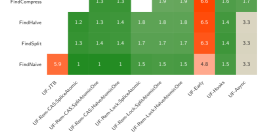
Figure 3. Relative performance of different union-find implementations on graphs used in our evaluation of ConnectIt in the No Sampling setting. The numbers are slowdowns relative to the fastest implementation.

4.1.1. Union-Find Evaluation

Figure 3 shows the relative performance of different union-find variants from ConnectIt in the No Sampling setting, averaged across all graphs. $\mathsf{UF\mathchar 45\relax Rem\mathchar 45\relax CAS}$ implementations achieve consistently high performance in this setting using either $\mathsf{SplitAtomicOne}$, $\mathsf{HalveAtomicOne}$, or $\mathsf{SpliceAtomic}$ to perform compression. The $\mathsf{UF\mathchar 45\relax Rem\mathchar 45\relax Lock}$ implementation is 1.5–1.9x slower than $\mathsf{UF\mathchar 45\relax Rem\mathchar 45\relax CAS}$ for all 6 variants of this algorithm. $\mathsf{UF\mathchar 45\relax Early}$, $\mathsf{UF\mathchar 45\relax Hooks}$, and $\mathsf{UF\mathchar 45\relax Async}$ are all slower on average: between 4.8–6.6x, 1.4–1.6x, and 1.7–3.3x on average, respectively. Finally, $\mathsf{UF\mathchar 45\relax JTB}$ is much slower, although the $\mathsf{FindTwoTrySplit}$ option only incurs a more modest slowdown of 4.2x on average.

Performance Analysis. We annotated our union-find algorithms to measure the Max Path Length (MPL), or the longest path length experienced by the union-find algorithm during the execution of any Union operation, and the Total Path Length (TPL), which is the sum of all path lengths observed during all Union executions. We also measured the number of LLC misses, and the total amount of bytes transferred to the memory controller (both reads and writes). We note that adding this instrumentation affects the overall running times between 10–20%. We report the detailed results of the analysis in Appendix C.1. We find that the TPL is relevant for predicting the running time—the TPL has a Pearson correlation coefficient of 0.738 with running time (the MPL has a weaker coefficient of 0.344).

Takeaways. Based on this discussion, we conclude that minimizing both the total amount of data written to and read from the memory controller, and improving the locality of these accesses, thereby reducing the number of LLC misses, is critical for high performance. One way of achieving these objectives is by minimizing the TPL, although optimizing to minimize the TPL does not by itself guarantee the fastest performance.

4.2. Performance With Sampling

We defer a detailed analysis of our performance under different sampling schemes to Appendix C.2, and list our main findings here. Our results for combining ConnectIt algorithms with different sampling schemes suggest the following takeaways when selecting algorithms and sampling schemes for different graphs:

• For low-diameter graphs, such as social networks and Web graphs, the fastest finish algorithms combined with all three sampling schemes explored in this paper provide significant speedups over the fastest ConnectIt algorithms that do not use sampling, ranging from 1.4–3.9x speedup using $k$-out Sampling (2.2x on average), 1.1–4.9x speedup using BFS Sampling (2.4x on average), and 0.98–4.6x speedup for LDD Sampling (2.3x on average).

• If the graph has high diameter, then using $k$-out Sampling with any union-find method seems to be the best fit, unless using label propagation, in which case BFS Sampling is the best choice.

• For large Web graphs, like the ClueWeb and the two Hyperlink graphs studied in this paper, all three sampling schemes result in very high speedups over the fastest unsampled algorithms in ConnectIt, ranging from 1.7–1.9x for $k$-out Sampling, 1.5–2.3x for BFS Sampling, and 1.7–2.4x for LDD Sampling. Furthermore, the fastest ConnectIt algorithm for these graphs is obtained by combining one of these sampling schemes with the $\mathsf{UF\mathchar 45\relax Rem\mathchar 45\relax CAS}$ algorithm (each scheme is fastest on one graph).

4.3. Comparison with State-Of-The-Art

Table 3 reports the performance of these systems on the inputs used in our evaluation. Aside from BFSCC and WorkeffCC (defined below), which we implemented as part of our system, we were unable to run the other systems on the large inputs due to the fact that these systems do not support compression, which is required for systems to compactly store and process our largest graph inputs on our machine without using an exorbitant amount of memory. We list the main takeaways of the experimental results here, and present detailed results of the comparison in Appendix C.3.

• BFSCC: The BFS-based connectivity implementation available from Ligra (Shun and Blelloch, 2014). This algorithm computes each connected component by running a parallel BFS from the vertex with the lowest ID within it. We find that using sampling, ConnectIt is between 1.22–80.0x faster than BFSCC, and 15.6x faster on average.

• WorkeffCC: The work-efficient connectivity implementation by Shun et al. (Shun et al., 2014), which recursively computes LDD (publicly available as part of GBBS (Dhulipala et al., 2018)). Our implementations without sampling are between 1.45–19.4x faster (5.6x faster on average). Our implementations with sampling are between 3.1–27.5x faster (9.03x faster on average). This algorithm previously held the record time for connectivity on the Hyperlink2012 graph on any system, running in 25.8 seconds on a 72-core machine. The fastest ConnectIt algorithm, $\mathsf{UF\mathchar 45\relax Rem\mathchar 45\relax CAS}$ with $\mathsf{SplitAtomicOne}$, is 3.14x faster on the same machine, and thus breaks this record.

• Multistep: The hybrid BFS/label propagation method by Slota et al. (Slota et al., 2014). Our codes without sampling are between 1.95–21.4x faster, and 10.1x faster on average. Using sampling, our codes are between 9.6–30.3x faster, and 18.6x faster on average. Our codes are much faster on large-diameter networks (over 1,000x faster).

• Galois: Galois is a state-of-the-art shared-memory parallel programming library (Nguyen et al., 2013). We found that their label propagation algorithm is consistently the fastest implementation in their code base, and report running times for this implementation for all but one graph (road_usa, discussed below).

  Our codes without sampling are between 1.78–3.69x faster than theirs (2.32x faster on average), and our codes using sampling are between 2.17–12.3x faster than theirs (6.21x faster on average). Our codes are 2.43x faster than their default (EdgetiledAsync) algorithm on the road_usa graph, which was their fastest algorithm for this graph.

• PatwaryRM: We compare with the multicore Rem’s algorithm by Patwary et al. (Patwary et al., 2012b). Our fastest implementations without sampling achieve between 1.27–2.87x speedup over their implementation (1.99x speedup on average), and our fastest implementations with sampling achieve between 2.09–6.28x speedup over their implementation (4.31x speedup on average).

• GAPBS: We compared with the GAP Benchmark Suite, a state-of-the-art shared-memory graph processing benchmark (Beamer et al., 2015), which implements the Afforest algorithm (Sutton et al., 2018). Our fastest implementations without sampling are between 0.33–4.17x faster than their Afforest (Sutton et al., 2018) implementation (2.08x faster on average). Our fastest implementations with sampling are between 1.32–8.55x faster than their Afforest implementation (3.9x faster on average).

Algorithm	RO	LJ	CO	TW	FR	RM	BA	CW	HL14	HL12
$\mathsf{UF\mathchar 45\relax Early}$	1.48e9	9.23e8	1.38e9	4.31e8	1.05e9	3.49e8	5.16e8	4.00e8	3.15e9	2.80e9
$\mathsf{UF\mathchar 45\relax Hooks}$	3.12e9	4.21e9	5.94e9	2.79e9	1.49e9	7.27e8	1.18e9	4.69e9	5.17e9	4.48e9
$\mathsf{UF\mathchar 45\relax Async}$	3.49e9	3.36e9	5.29e9	2.73e9	1.41e9	8.05e8	1.13e9	4.86e9	5.92e9	4.69e9
$\mathsf{UF\mathchar 45\relax Rem\mathchar 45\relax CAS}$	3.98e9	5.28e9	7.16e9	3.85e9	2.01e9	8.78e8	1.46e9	5.73e9	6.64e9	5.64e9
$\mathsf{UF\mathchar 45\relax Rem\mathchar 45\relax Lock}$	1.56e9	3.68e9	5.95e9	3.36e9	1.74e9	7.67e8	1.42e9	3.56e9	2.99e9	3.21e9
$\mathsf{UF\mathchar 45\relax JTB}$	1.15e9	1.06e9	2.68e9	1.42e9	7.33e8	2.88e8	5.27e8	2.15e9	2.26e9	1.79e9
$\mathsf{Liu\mathchar 45\relax Tarjan}$	2.87e8	4.31e8	5.98e8	3.77e8	1.84e8	1.11e8	1.98e8	3.02e8	2.80e8	2.62e8
$\mathsf{SV}$	1.79e8	4.56e8	1.13e9	2.89e8	1.76e8	1.06e8,	2.43e8	3.34e8	2.65e8	2.24e8

Table 4. Maximum parallel streaming throughput (directed edge insertions per second) achieved by ConnectIt streaming algorithms on our graph inputs, and two synthetic graph inputs from the RMAT (RM) and Barabasi-Albert (BA) families. Due to memory constraints, we were unable to materialize a COO representation of our three largest graphs, and instead, sample 10% of the edges to use in the batch. Otherwise, the entire graph is used as part of a single batch, which is not permuted. Note that there are no queries in the batch. For each graph we display the algorithm with the highest throughput in bold.

4.4. Streaming Parallel Graph Connectivity

Experiment Design. We run two types of streaming experiments. The first type generates a stream of edge insertions by sampling a fraction of the edges ($f_{u}$) from a static input graph to use as insertions. Unless otherwise mentioned, we use all edges as insertions ($f_{u}=1$). The second type uses synthetic graph generators to sample edge insertions. We consider the RMAT and Barabasi-Albert (BA) graph generators (Bader and Madduri, 2006; Barabási and Albert, 1999) in these experiments. We generate RMAT graphs using the parameters $(a,b,c)=(0.5,0.1,0.1)$. In both the RMAT and BA graphs, the number of vertices is $n=2^{30}$ and the number of edges is $10n$. For both graphs, the batches used by our streaming algorithms are represented in the COO format. For the ClueWeb, Hyperlink2014, and Hyperlink2012 graphs, we are unable to represent the entire graph in COO, and sample 10% of the edges to use as insertions.

4.4.1. Streaming Throughput

We first consider the throughput achieved by each algorithm family in the setting where only insertions are applied. Table 4 reports the streaming throughput achieved by the fastest variant of each algorithm on each graph. Note that no sampling is applied in these streaming experiments. The insertions are streamed as part of a single, large batch, which is applied by the algorithm in parallel for Type (1) and (2), and separately applied for insertions first, then queries second, for Type (3) algorithms (see the discussion on these types in Section 3.5).

The performance of most of our union-find algorithms is consistently high on these graphs, in particular the performance of $\mathsf{UF\mathchar 45\relax Hooks}$, $\mathsf{UF\mathchar 45\relax Async}$, $\mathsf{UF\mathchar 45\relax Rem\mathchar 45\relax CAS}$, and $\mathsf{UF\mathchar 45\relax Rem\mathchar 45\relax Lock}$. As in the static setting, the $\mathsf{UF\mathchar 45\relax Rem\mathchar 45\relax CAS}$ algorithm consistently performs the best across all input graphs, achieving a maximum throughput of over 7 billion edge insertions per second on the com-Orkut graph. The other two union-find algorithms, $\mathsf{UF\mathchar 45\relax Early}$ and $\mathsf{UF\mathchar 45\relax JTB}$, achieve somewhat inconsistent performance, which is consistent with our findings from Section 4.1. For $\mathsf{UF\mathchar 45\relax Early}$, the version of the algorithm with no extra compression performed best compared with the versions that perform additional path compression algorithms, as in the static case in Figure 3 (comparing $\mathsf{FindNaive}$ performance to that of non-trivial path compression options). The performance of $\mathsf{SV}$ seems to depend mostly on the number of rounds required (more rounds on larger diameter networks like road_usa). We note that the algorithm requires just two rounds on com-Orkut. The performance of the fastest $\mathsf{Liu\mathchar 45\relax Tarjan}$ algorithm is similar to that of the $\mathsf{SV}$ algorithm in the streaming setting across all graphs. Both of these methods are significantly slower than the fastest union-find methods. We note that the fastest $\mathsf{Liu\mathchar 45\relax Tarjan}$ algorithm in this setting is consistently the version using $\mathsf{Connect}$, $\mathsf{RootUp}$, $\mathsf{FullShortcut}$, and $\mathsf{Alter}$ (the $\mathsf{CRFA}$ algorithm in Appendix D).

Batch Size	STINGER	Updates/sec	ConnectIt	Updates/sec
10	6.07e-2	164	2.14e-6	4.67M
$10^{2}$	9.87e-2	1013	1.19e-5	8.40M
$10^{3}$	0.171	5,847	2.19e-5	45.6M
$10^{4}$	0.137	72,992	5.19e-5	192M
$10^{5}$	0.503	198,807	3.25e-4	307M
$10^{6}$	3.99	250,626	2.73e-3	366M
$2\cdot 10^{6}$	6.52	306,748	4.313e-3	463M

Table 5. Running times (seconds) and edge insertion rates (directed edges/second) for STINGER’s dynamic connected components algorithm and ConnectIt’s $\mathsf{UF\mathchar 45\relax Rem\mathchar 45\relax CAS}$ algorithm (with $\mathsf{SplitAtomicOne}$) when performing batch edge insertions on an empty graph with varying batch sizes. Inserted edges are sampled from the RMAT graph generator.

4.4.2. Streaming Comparison with STINGER

STINGER is based on a dynamic data structure for representing dynamic graphs in the streaming setting (Ediger et al., 2012). STINGER supports a dynamic connected components algorithm by McColl et al. (McColl et al., 2013). Their algorithm also supports edge deletions, which makes it more general than our algorithms. Since our codes do not update the graph structure, for the sake of comparing STINGER with our codes, we only report the time required for STINGER to update its connectivity labeling, which is strictly less than the overall update time of STINGER. As far as we know, the only existing parallel algorithm designed for incremental connectivity is by Simsiri et al. (Simsiri et al., 2017), but unfortunately we were unable to obtain the code from the authors.

Comparison. The STINGER code takes a parameter which trades off space usage with the amount of re-computation that has to be done upon an update (edge insertion or deletion). We set it to the lowest possible value, which gave the best performance. We note that the STINGER dynamic connectivity algorithm has an unusually long initialization period, which depends on the number of vertices. We were unable to initialize the STINGER dynamic connectivity algorithm within several hours for graphs with more than 1 million vertices, and were only able to evaluate batches of size up to 2 million due to limitations in their system. Based on this, we opted to generate batches from an RMAT graph generator using $2^{20}$ vertices. Our experiment inserts batches of varying sizes and measures the time required by the dynamic connectivity algorithm to process the batch. The times we report ignore the time taken by STINGER to update adjacency information.

Table 5 reports the results of the experiments for STINGER and for ConnectIt’s $\mathsf{UF\mathchar 45\relax Rem\mathchar 45\relax CAS}$ algorithm with the $\mathsf{SplitAtomicOne}$ option. Both implementations are run on the same machine using all cores with hyper-threading. ConnectIt significantly outperforms STINGER in this setting, achieving between 1,461–28,364x speedup across different batch sizes. Surprisingly, ConnectIt applied with a batch size of 10 achieves significantly higher throughput than STINGER for a batch size of 2M. We realize that our comparison is somewhat unfair toward STINGER, since although this implementation is one of the fastest batch-incremental connectivity implementations currently publicly available, it is designed for both edge insertions and deletions, and must perform extra work in anticipation of edge deletions, which our algorithms do not handle.

4.5. Algorithm Selection in ConnectIt

Given a graph, which combination of ConnectIt’s sample and finish methods should one apply to obtain the best performance?

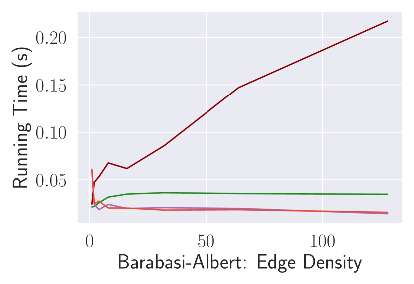
(a)

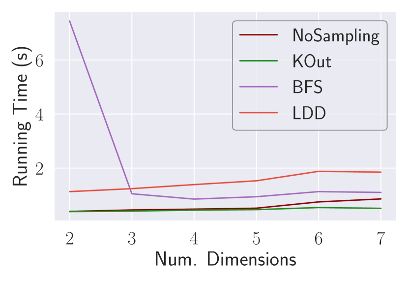
(b)

Figure 4. Running times (seconds) of the $\mathsf{UF\mathchar 45\relax Rem\mathchar 45\relax CAS}$ algorithm with $\mathsf{SplitAtomicOne}$ and $\mathsf{FindNaive}$ using different sampling methods on two synthetic graph families. Subfigure 4(a) displays results for graphs drawn from the Barabasi-Albert generator where the $x$-axis specifies the edge density, or the number of edges drawn for each newly added vertex. Subfigure 4(b) shows results for $d$-dimensional torii where the $x$-axis shows the dimension.

Evaluation on Synthetic Networks. To provide guidance, we evaluated $\mathsf{UF\mathchar 45\relax Rem\mathchar 45\relax CAS}$ with $\mathsf{SplitAtomicOne}$ and $\mathsf{FindNaive}$, which are consistently ConnectIt’s fastest connectivity methods, on two synthetic graph families with significantly different properties. Figure 4(a) displays results for graphs drawn from the Barabasi-Albert (BA) generator on $10^{7}$ vertices, varying the edge density of the graphs in powers of two from $1$ to $128$. Figure 4(b) displays results for $d$-dimensional torii on $10^{9}$ vertices where we vary the dimension of the grid (each vertex is connected to its $2d$ adjacent neighbors).

The diameter of the BA graphs decreases with increasing density, and as a result both BFS and LDD Sampling achieve good performance as the density increases. Both schemes use the direction-optimization technique used when traversing frontiers (Beamer et al., 2012; Shun and Blelloch, 2013), which is beneficial in high-density graphs. For the sparse (high-diameter) case where $n=m$, we found that $k$-out Sampling and not using sampling were the fastest.

For $d$-dimensional torii, $k$-out Sampling consistently performs the best across the range of $d$ that we evaluate. For small $d$, there is little difference between $k$-out Sampling and no sampling, but for larger $d$, and thus higher average degree, $k$-out Sampling begins to achieve significant speedups over no sampling. The performance of BFS Sampling is poor on this graph family since the diameter of the $d$-dimensional torus is $O(n^{1/d})$, causing BFS to perform many rounds. The performance of LDD Sampling is also poor, since the induced clustering consists of many small clusters and thus most of the vertices must be processed in the finish phase.

Picking an Algorithm. Based on both our evaluation on the synthetic graph families above, and the results for a broad collection of large real-world graphs shown in Table 3, we devised a decision tree that can help users select an appropriate algorithm, which we show in Figure 5. We recommend using the $\mathsf{UF\mathchar 45\relax Rem\mathchar 45\relax CAS}$ algorithm, with any of the three possible splice strategies in combination with the $\mathsf{FindNaive}$ strategy. Based on our evaluation of union-find algorithms in Section 4.1.1, this family of algorithms is consistently the fastest. Regarding sampling, for extremely sparse networks with low average degree such as road_usa $(m/n<3)$, not using sampling can be beneficial. The reason is that the cost of simply going over this small set of edges twice during two-phase execution outweighs the additional benefit provided by sampling, since we almost finish computing connectivity after applying $k$-out Sampling. On the other hand, if the graph is reasonably dense, and also has low diameter, either BFS or LDD Sampling can obtain the best results. Finally, if the graph diameter is unknown, or known to be high, then we recommend using $k$-out Sampling.

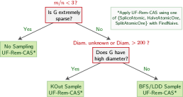
Figure 5. Decision tree for selecting a ConnectIt algorithm based on the input graph properties. The text shown in red are suggested (heuristic) decision rules derived from our evaluation.

5. Applying ConnectIt

In this section, we examine how ConnectIt can be used to accelerate graph processing in two important graph applications.

5.1. Approximate Minimum Spanning Forest

Computing a minimum spanning forest (MSF) of a weighted undirected graph is an important problem, and some popular graph clustering algorithms including single linkage, and affinity clustering can be viewed as post-processing of a graph’s minimum spanning forest (Manning et al., 2008; Bateni et al., 2017). We consider the closely related problem of computing an approximate MSF, and show how a folklore approach can be accelerated using ConnectIt.

Definition. Consider a weighted graph $G(V,E,w)$. Let $\mathcal{F}_{\mathsf{OPT}}$ represent any spanning forest of $G$ of minimum weight. The approximate minimum spanning forest (AMSF) problem is to compute a spanning forest $\mathcal{F}_{\mathsf{APX}}$ of $G$, where $W(\mathcal{F}_{\mathsf{OPT}})\leq W(\mathcal{F}_{\mathsf{APX}})\leq(1+\epsilon)W(\mathcal{F}_{\mathsf{OPT}}).$ We make the standard assumption that the weights are polynomially-bounded, i.e., $\exists c$ s.t. $\forall e\in E,w(e)=O(n^{c})$ for some constant $c$.

Algorithm. The following is a folklore algorithm for the AMSF problem. Let $W_{\min}=\min_{e\in E}w(e)$. Bucket the edges of $G$, such that the $i$’th bucket contains edges with weight in the range $[W_{\min}(1+\epsilon)^{i},W_{\min}(1+\epsilon)^{i+1})$. As the weights in $G$ are polynomially bounded, there are $O(\log_{1+\epsilon}n)$ buckets. The algorithm maintains a connectivity labeling $\mathcal{C{}}$, which is updated as it processes the buckets from smallest to largest weight. For the $i$’th bucket, it first removes all edges that are self-loops. It then computes a spanning forest $\mathcal{F}_{i}$ on the remaining edges in the bucket, and updates the connectivity labeling so that $\mathcal{C{}}$ represents the connected components of $\cup_{j=0}^{i}\mathcal{F}_{j}$. The final minimum spanning forest is simply the union of all of the computed spanning forests.

Variants. We consider several variants of the algorithm above:

1. $\mathsf{AMSF}\mathchar 45\relax\mathsf{COO}$ is a direct implementation of the algorithm described above, which works by writing the edges in the graph into the COO format, which is then sorted by weight. The buckets are represented using $O(\log n)$ pointers into this array.

2. $\mathsf{AMSF}\mathchar 45\relax\mathsf{F}$ avoids extracting all of the edges into COO, and instead extracts the buckets in COO format one at a time from input graph (in CSR representation). The extracted edges are removed (filtered out) from the CSR representation, and at the end of the algorithm, the CSR graph has no remaining edges.

3. $\mathsf{AMSF}\mathchar 45\relax\mathsf{NF}$ works similarly to $\mathsf{AMSF}\mathchar 45\relax\mathsf{F}$, with the exception that the graph is not mutated when extracting edges (and thus all edges in the graph are inspected in every round).

For the $\mathsf{AMSF}\mathchar 45\relax\mathsf{NF}$ variant, we consider applying a sampling optimization similar to the one used in ConnectIt, which we refer to as $\mathsf{AMSF}\mathchar 45\relax\mathsf{NF}\mathchar 45\relax\mathsf{S}$. The idea is to compute, in each round, the largest connected component in the connectivity labeling, $L_{\max}$, and to skip processing vertices in the $L_{\max}$ component and their incident edges when searching for the spanning forest over edges in the current round. This optimization is correct, since any edge emanating out of the $L_{\max}$ component that is skipped will be considered from the other endpoint, which will not be skipped.

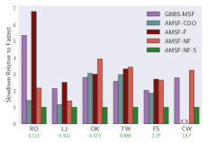
Figure 6. Relative performance of the AMSF algorithms with $\epsilon=0.25$. The values on the $y$-axis are normalized to the running time of the fastest algorithm; this time in seconds is shown below the name of each graph in green. Methods resulting in failure are marked with a red $\mathsf{x}$.

Experimental Results. We evaluated all of the AMSF variants above over weighted versions of our unweighted graph inputs by adding random weights drawn from an exponential distribution with a constant mean. We set $\epsilon=0.25$. We did not evaluate weighted versions of the Hyperlink graphs due to storage constraints in our experimental environment. All AMSF variants use the $\mathsf{UF\mathchar 45\relax Rem\mathchar 45\relax CAS}$ method with $\mathsf{SplitAtomicOne}$ and $\mathsf{FindNaive}$ to concurrently update the connectivity labeling when processing edges within a bucket. We compare these variants to $\mathsf{GBBS}\mathchar 45\relax\mathsf{MSF}$, an exact minimum spanning forest (MSF) algorithm from GBBS (Dhulipala et al., 2018), which is a CSR-based implementation of Borůvka’s algorithm. To the best of our knowledge, $\mathsf{GBBS}\mathchar 45\relax\mathsf{MSF}$ is the fastest existing multicore MSF algorithm.

Figure 6 shows our results. Other than the two smallest graphs, no AMSF variant without sampling outperforms the $\mathsf{GBBS}\mathchar 45\relax\mathsf{MSF}$ algorithm by a significant margin. For $\mathsf{AMSF}\mathchar 45\relax\mathsf{COO}$, the primary reason for its poor performance on large graphs is the large overhead of sorting and processing edges stored in COO. $\mathsf{AMSF}\mathchar 45\relax\mathsf{F}$ suffers for similar reasons, since a large fraction of the edges fall into the first few buckets, which are explicitly stored in COO. Both $\mathsf{AMSF}\mathchar 45\relax\mathsf{COO}$ and $\mathsf{AMSF}\mathchar 45\relax\mathsf{F}$ fail due to memory allocation errors on the ClueWeb graph for this reason. $\mathsf{AMSF}\mathchar 45\relax\mathsf{NF}\mathchar 45\relax\mathsf{S}$ consistently attains the best performance across all graphs, obtaining between 2.03–5.36x speedup over the exact algorithm (2.95x on average), since it quickly finds a partial spanning forest spanning most of the largest connected component after processing the first few buckets, and can skip processing vertices in this component in subsequent rounds.

5.2. Index-Based SCAN

The Structural Clustering Algorithm for Networks (SCAN) clustering algorithm (Xu et al., 2007) clusters graphs using the idea that ‘similar’ vertices have similar neighbor sets, e.g., using a similarity measure such as cosine similarity. SCAN is defined using two parameters: a similarity threshold $\epsilon\in[0,1]$ and $\mu\geq 2$. Two vertices are said to be $\epsilon$-similar if their similarity is at least $\epsilon$. A vertex is a core vertex if it has at least $\mu$ neighbors that it is $\epsilon$-similar to. The objective is to find a maximal clustering where all vertices within a cluster are connected over a path of $\epsilon$-similar edges.

GS*-Index and GS*-Query (Wen et al., 2017). Motivated by the fact that often one is interested in finding multiple clusterings with varying $\epsilon$ and $\mu$, the GS*-Index (Wen et al., 2017) algorithm builds an index structure so that cluster retrieval can be quickly performed using the index. Once the index has been computed, for a given $\epsilon$ and $\mu$ the query algorithm, GS*-Query (Algorithm 4 in (Wen et al., 2017)), performs a sequential search from the core vertices, considering only $\epsilon$-similar edges.

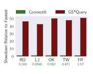
Figure 7. Relative performance of our parallel implementation of GS*-Query using ConnectIt, and GS*-Query when searching for a clustering with $\epsilon=0.1$ and $\mu=3$. The fastest running time in seconds for each graph is shown in green.

Experimental Results. We parallelized the GS*-Query algorithm with ConnectIt using the $\mathsf{UF\mathchar 45\relax Rem\mathchar 45\relax CAS}$ algorithm with $\mathsf{FindNaive}$ and $\mathsf{SplitAtomicOne}$, and compared the parallel query algorithm to the sequential GS*-Query algorithm. Figure 7 shows the results of our evaluation for $\epsilon=0.1$ and $\mu=3$ on a subset of our graph inputs. The index requires $O(m)$ space (with a significant constant), and so we were unable to evaluate it on our larger graph inputs. Our results show that by using ConnectIt, we can obtain between 42.5–50.5x speedup (47.4x on average) over the original sequential GS*-Query, potentially enabling an order of magnitude more clusterings to be evaluated by users. We have recently also parallelized the index construction algorithm (GS*-Index) (Tseng et al., 2021).

6. Conclusion

We have introduced the ConnectIt framework, which provides orders of magnitude more parallel static and incremental connectivity and spanning forest implementations than what currently exist today. We have found that the fastest multicore implementations in ConnectIt significantly outperform state-of-the-art parallel solutions. We believe that this paper is one of the most comprehensive evaluation of multicore connectivity implementations to date.

Appendix A Appendix Overview

The appendix is structured as follows:

1. Section B contains deferred content and proofs about the ConnectIt framework.

   1. Section B.1 contains correctness proofs for our sampling algorithms.

   2. Section B.2 contains correctness proofs about our finish algorithms, as well as more information about our Shiloach-Vishkin, Stergiou, and Label Propagation algorithms.

   3. Section B.3 describes the ConnectIt framework for spanning forest.

   4. Lastly, Section B.4 describes the ConnectIt framework for streaming in the batch-incremental and wait-free asynchronous settings.

2. Section C contains deferred experimental results including:

   1. Results about ConnectIt algorithms in the setting without sampling (Section C.1). This includes a performance characterization of our union-find and Liu-Tarjan algorithms based on performance counters and other metrics.

   2. Results about ConnectIt algorithms in the setting with sampling (Section C.1).

   3. Additional details about the experimental comparisons to state-of-the-art algorithms done in this paper (Section C.3).

   4. An experimental evaluation of the sampling schemes considered in this paper, analyzing how adjusting their parameters affects their running time, and the sampling quality (Section C.5).

   5. A comparison between ConnectIt algorithms, and basic graph processing primitives that map, and perform indirect reads across all edges (Section C.5.1).

   6. A comparison between ConnectIt algorithms on very large graphs, and existing state-of-the-art results for such large graphs (Section C.6).

3. For completeness, we provide pseudocode for our algorithms (Section D).

Additional Primitives. We define an additional primitive used in the following sections: a writeMin takes two arguments, a memory location x and a value val. If val is less than the value stored at x, then writeMin atomically updates the value at x to val and returns true; otherwise it returns false. A writeMin can be implemented with a loop that attempts a CAS as long as val is less than the value at x (Shun et al., 2013).

Appendix B Framework

In this section, we provide deferred correctness proofs, as well as descriptions of algorithms deferred from the main body of the paper.

B.1. Correctness for Sampling Algorithms

Theorem 1.

$k$-out Sampling, BFS Sampling, and LDD Sampling all produce connectivity labelings satisfying Definition 1.

Proof.

Recall that Definition 1 requires that the labeling $C{}$ emitted by the sampling method is a valid partial connectivity labeling (i.e., if two vertices $u,v\in V$ are in the same tree in $C$, then they are connected in $G$). BFS Sampling satisfies this requirement since the labeling represents a single connected component which is clearly a valid partial labeling. Similarly, LDD Sampling satisfies this definition since the labeling is precisely the contraction induced by the low-diameter decomposition clustering, and it is easy to check that this is a valid partial labeling. Finally, since we use a linearizable union-find algorithm as our sub-routine in $k$-out Sampling, a proof almost identical to that of Theorem 2 shows that the labeling induced by $k$-out Sampling is a correct partial labeling of $G$. ∎

B.2. Finish Algorithms

We now finish describing our ConnectIt finish methods and providing deferred correctness proofs for our finish methods. We start with the correctness proofs for linearizably monotonic methods.

B.2.1. Correctness for Linearizably Monotonic Methods

Theorem 2.

The connectivity algorithm in ConnectIt (Algorithm 1) applied with a sampling method $\mathcal{S}$ satisfying Definition 1 and a linearizably monotone finish method $\mathcal{F}$ is correct.

Proof.

Let $C{}$ be the partial labeling produced by the sampling method $\mathcal{S}$. Now, consider $\mathcal{F}$, which is a linearizably monotone finish method operating on the partial connectivity labeling $C{}$. Since we are handling an abstract connectivity algorithm $\mathcal{F}$, it is helpful to think about operations of two types: (i) those that try to “apply” an edge $(u,v)$ (i.e., it checks whether $u$ and $v$ are in different trees, and if so changes the labeling so that $u$ and $v$ are in the same tree in the new labeling), and (ii) lower-level operations that compress trees. Furthermore, note that $\mathcal{F}$ will avoid applying (directed) edges coming out of $L_{\max}{}$, which could be problematic since there may be many edges of the form $(u,v)$ where $u\in L_{\max}{}$ and $v\notin L_{\max}{}$ that must be examined to compute a correct labeling. However, since the graph is symmetric, $\mathcal{F}$ does apply all such inter-cluster edges, since such edges will be applied while processing vertex $v\notin L_{\max}{}$, which is contained in some initial component $c\neq L_{\max}{}$. The algorithm must process this component, since it only skips applying the directed edges incident to vertices in component $L_{\max}{}$.

Consider the linearization order of the finish algorithm $\mathcal{F}$. Before running $\mathcal{F}$, the labeling $C{}$ represents some set of intermediate clusters that is a partial connectivity labeling of $G$ (i.e., if there is a path between two vertices $u$ and $v$ in the trees represented by the labeling $C{}$, then this implies that there is a path between $u$ and $v$ in $G$). We will show by induction on the linearization order that each operation preserves the fact that $C{}$ is a partial connectivity labeling of $G$. Consider the two types of operations:

• Operations of type (ii) described above are trivial to handle since the operations only change the structure of the labeling, and not the connectivity information represented by it. Thus, the labeling is still a valid partial connectivity labeling of $G$.

• Next, consider an operation of type (i), which applies an edge $(u,v)$. If $u$ and $v$ are in the same tree before the operation, the operation does not modify the structure of the trees and thus the new connectivity labeling (if any labels changed) is equivalent to the previous labeling (and is thus valid). Otherwise, if $u$ and $v$ are in different trees, the operation will produce a new labeling where $u$ and $v$ are in the same tree, and the labeling for any vertices $z$ not in the same tree as either $u$ or $v$ is unmodified. Thus, the new labeling is a partial connectivity labeling of $G$, since the algorithm only changes labels of vertices in the trees containing $u$ and $v$, and by induction all vertices in each of $u$’s and $v$’s trees were connected by paths in $G$, and due to the $(u,v)$ edge, all vertices in the union of these trees have paths between each other in $G$.

Therefore, at the end of the execution, the algorithm has computed a partial connectivity labeling, and has linearized the apply operations of all $(u,v)$ edges, where $u$ and $v$ are not both in $L_{\max}{}$. Note that all edges $(u,v)$, where both $u$ and $v$ are initially in $L_{\max}{}$ are initially in the same tree. Therefore, the algorithm has computed a connectivity labeling, having applied all edges $(u,v)\in E$, and so for any $u,v\in V$, $u$ and $v$ are in the same tree in $C{}$ if and only if there is a path between $u$ and $v$ in $G$, completing the proof. ∎

B.2.2. Correctness Properties of Rem’s Algorithm

Theorem 3.

$\mathsf{UF\mathchar 45\relax Rem\mathchar 45\relax CAS}$ and $\mathsf{UF\mathchar 45\relax Rem\mathchar 45\relax Lock}$ are correct connectivity algorithms in the phase-concurrent setting, and result in linearizable results for a set of phase-concurrent union and find operations.

Proof.

We provide a high-level proof sketch. The proof is based on building a graph of completed and currently active union operations. Let this graph be $G_{C}$. The graph (roughly) corresponds to the trees concurrently maintained by the algorithm, and includes extra edges corresponding to the currently executing Union operations.

• When a $\textsc{Union}(u,v)$ operation starts (is invoked), we place a shadow edge between the root of the tree currently containing $u$ and the tree currently containing $v$.

• When a $\textsc{Union}(u,v)$ operation completes (we receive its response), we first check if it returns $\mathsf{True}$ due to atomically hooking a tree root $r_{u}$ to a vertex $h_{v}$. If so, we link the tree containing $r_{u}$ to $h_{v}$ in the graph. Then, we remove the shadow edge corresponding to this Union operation from the graph.

The proof is by induction on the completion times of the operations that (i) once a $\textsc{Union}(u,v)$ call completes, $u$ and $v$ always remain connected in $G_{C}$ and (ii) any vertices $u$ and $v$ in different components in $G$ are never connected in $G_{C}$. The proof is similar to that of Theorem 2. ∎

B.2.3. Counter-example for Rem’s Algorithm with SpliceAtomic and FindCompress

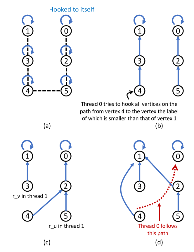
Figure 8. A counter example of Rem’s algorithm with $\mathsf{SpliceAtomic}$ and $\mathsf{FindCompress}$.

As mentioned in Section 3.3, combining the $\mathsf{Find-}$ $\mathsf{Compress}$ option with the $\mathsf{SpliceAtomic}$ rule in the $\mathsf{UF\mathchar 45\relax Rem\mathchar 45\relax Lock}$ and $\mathsf{UF\mathchar 45\relax Rem\mathchar 45\relax CAS}$ algorithms results in incorrect connectivity algorithms. Figure 8 illustrates a counter-example for these algorithms. Without loss of generality, we will explain why $\mathsf{UF\mathchar 45\relax Rem\mathchar 45\relax Lock}$ can lead to an incorrect result with $\mathsf{FindCompress}$ and $\mathsf{SpliceAtomic}$ (the counter-example is identical for $\mathsf{UF\mathchar 45\relax Rem\mathchar 45\relax CAS}$).

Consider the following input graph where $V=\{0,1,2,3,4,5\}$ and $E=\{(0,2),(1,3),(2,5),(3,4),(4,5)\}$ (shown in Figure 8 (a)). Assume the $\mathsf{UF\mathchar 45\relax Rem\mathchar 45\relax Lock}$ algorithm is applied to the edges $(2,5)$ and $(0,2)$ sequentially. After that, thread 0 applies $\mathsf{UF\mathchar 45\relax Rem\mathchar 45\relax Lock}$ to the edge $(3,4)$, and is about to execute Line 11 in Algorithm 8 (i.e., thread 0 is in the process of executing $\mathsf{FindCompress}$ (Line 17 in Algorithm 13)).

In the meantime, suppose another thread finishes applying $\mathsf{UF\mathchar 45\relax}$ $\mathsf{Rem\mathchar 45\relax Lock}$ to the edge $(1,3)$. The state of the trees at this point in the execution is shown in Figure 8 (b). The only outstanding operation is in thread 0, which will still execute $\mathsf{FindCompress}$ from vertex $4$.

Now, thread 1 applies $\mathsf{UF\mathchar 45\relax Rem\mathchar 45\relax Lock}$ to the edge $(4,5)$: after one iteration of while statement (Line 6 in Algorithm 13), $P[4]$ is changed from 3 to 2, and $r_{u}=5$, $r_{v}=3$ (Figure 8 (c)).

After that, thread 0 executes the while loop (Line 11 in Algorithm 8), which hooks $P[4]$ and $P[2]$ to 1 (Figure 8 (d)); $P[0]$ is not hooked to vertex $1$ as $P[0]=0<1$.

Therefore vertex 0 is now isolated, and so thread 1 cannot link vertex 1 to any other vertices during $\mathsf{UF\mathchar 45\relax Rem\mathchar 45\relax CAS}$. Thus, the number of connected components after applying $\mathsf{UF\mathchar 45\relax Rem\mathchar 45\relax Lock}$ is 2, which is incorrect.

Additional Finish Methods

B.2.4. Shiloach-Vishkin

We include Shiloach-Vishkin’s algorithm (Shiloach and Vishkin, 1982) in ConnectIt, which is a classic parallel connectivity algorithm. The algorithm works by combining vertices into trees over a series of synchronous rounds using linking rules. Since only roots of trees can be linked (from larger root to smaller), the algorithm is naturally monotonic.

We provide pseudocode for our implementation of Shiloach-Vishkin in Algorithm 15 in Appendix D. The algorithm iteratively hooks roots of trees onto each other and compresses these trees by linking all vertices to the root of the tree. Each round of the algorithm maps over all edges. If an edge goes between two tree roots, the algorithm tries to hook the larger root to the smaller one. This operation can either be done using a plain write, which is what existing implementations of Shiloach-Vishkin use, or using the atomic writeMin operation to hook to the lowest incident root, which is what our algorithm does. A round ends by making the parent pointers of all vertices point to the root of their tree using pointer jumping. By considering the hook operations the algorithm tries to apply to each edge as a set of concurrent union operations, it is easy to show that this algorithm is linearizable, and thus linearizably monotonic, since it only links tree roots. Overall, our implementation of Shiloach-Vishkin requires $O(\log n)$ rounds, and each round can be implemented in $O(n+m)$ work and $O(\log n)$ depth. The overall work and depth of the algorithm are $O((n+m)\log n)$ and $O(\log^{2}n)$ respectively.

B.2.5. Stergiou

Stergiou et al. (Stergiou et al., 2018) presented a simple connectivity algorithm for the bulk synchronous parallel (BSP) model. Stergiou’s algorithm is nearly expressible in the Liu-Tarjan framework, with the exception that the algorithm uses two parents arrays, prevParent and curParent, instead of just one array as in the Liu-Tarjan algorithms. In each round, the algorithm first updates prevParent to be equal to curParent. It then performs a $\mathsf{ParentConnect}$, updating curParent based on the parent information in prevParent. Finally, it applies $\mathsf{Shortcut}$ on curParent and repeats until the parent array no longer changes. This algorithm is similar to the $\mathsf{PUS}$ algorithm of Liu-Tarjan, except that it uses two parent arrays instead of a single array. Stergiou’s algorithm is not monotonic since the algorithm can relabel non-root vertices in the parents array. The correctness proof for this algorithm is similar to the one for the Liu-Tarjan framework. We compose Stergiou’s algorithm with sampling methods in the same way as with the Liu-Tarjan framework.

B.2.6. Label Propagation

Label propagation is arguably the most frequently implemented parallel graph connectivity today, and has been implemented by many existing popular graph processing systems, including Pregel, Giraph, and other frameworks (Malewicz et al., 2010; Giraph, 2012; Nguyen et al., 2014; Shun and Blelloch, 2013; Zheng et al., 2015). The label propagation algorithm can be viewed as iterative sparse-matrix vector multiplication (SpMV), where the product is done over the $(\min,\min)$ semiring.

The implementation of this algorithm works as follows. Initially, each vertex is its own parent (we interpret the parents in the algorithm as the labels). In each round, the algorithm maintains a subset of vertices called a frontier that had their parent change in the previous round (at the start of the algorithm, this set contains all vertices). Then, in each round, the algorithm processes all edges incident to vertices in the current frontier, writing the minimum parent ID to the neighbors using a writeMin. The algorithm terminates once the array of parents no longer changes, which will occur within $D$ rounds where $D$ is the diameter of the graph. In the worst case, the algorithm will process all edges in each round giving overall work $O(mD)$ and depth $(D\log n)$. Note that the label propagation algorithm is not monotonic, since the label updates only affect the 1-hop neighborhood of a vertex spreading its label, and not entire trees.

The correctness of this algorithm is folklore, but we provide a generic proof of correctness for it, and other min-based algorithms like Liu-Tarjan and Stergiou’s algorithm in Theorem 5 below. We compose label propagation with sampling methods by using the same idea as with our sampled Liu-Tarjan framework, since relabeling the largest component to have the smallest ID ensures that vertices in this component never change their ID in subsequent rounds.

Correctness for Other Min-Based Methods

We start by abstractly defining the other min-based finish methods, which captures Liu-Tarjan’s algorithms, label propagation, and Stergiou’s algorithm.

Definition B.0.

An other min-based finish method is a round-based algorithm that repeatedly performs an “application” step on all edges. An edge application takes an edge $(u,v)$ and may update $P[u]$ (resp. $P[v]$) based on $P[v]$ (resp. $P[u]$), where a parent value is updated if and only if the new value is strictly smaller than the previous value. The algorithm terminates once the parent values stop changing.

Label propagation, Liu-Tarjan’s algorithms, and Stergiou’s algorithms all satisfy this definition. The following theorem states that composing other min-based algorithms with sampling algorithms produces correct results in ConnectIt.

Theorem 5.

The connectivity meta-algorithm in ConnectIt (Algorithm 1) applied with a sampling method $\mathcal{S}$ satisfying Definition 1 and an other min-based finish method $\mathcal{F}$ produces a correct connectivity labeling.

Proof.

The proof is by contradiction. Let $C{}$ be the labels produced by $\mathcal{S}$ satisfying Definition 1, that is they are consistent with some contraction of $G$ such that composing the contraction with the connectivity induced by inter-component edges results in a correct connectivity labeling of $G$. The proof only relies on the fact that the sampling method only maps vertices to the same label in $C{}$ if they are in the same component. Let $C{}^{\prime}$ be the final connectivity labeling after running $\mathcal{F}$.

Suppose that two vertices $u$ and $v$ in the same component in $G$ are assigned different labels in $C{}^{\prime}$. Since $u$ and $v$ are connected, there is a path between them in $G$, and on this path, there must be an edge $(x,y)$ where $C{}^{\prime}[x]\neq C{}^{\prime}[y]$. However, since the other min-based method $\mathcal{F}$ applies all edges in each round, on the last round it must have applied the $(x,y)$ edge, and since $C{}^{\prime}[x]\neq C{}^{\prime}[y]$, one of these values must have changed in this round, contradicting the assumption that this was the last round of the algorithm.

Furthermore, the other min-based algorithms composed with sampling methods can skip the edges incident to the largest sampled component, since the largest sampled component is relabeled to have the smallest ID, and thus by the preceding argument, all vertices that are connected to the largest sampled component in $G$ will eventually acquire its ID. ∎

B.3. ConnectIt: Spanning Forest

In this section, we show how to extend ConnectIt to solve the problem of generating a spanning forest of the graph. Algorithm 2 shows the generic ConnectIt algorithm for this problem. Like our connectivity algorithm, the algorithm can be supplied with different combinations of sample and finish methods and generate correct spanning forest algorithms. The main idea in the algorithm is to map each edge in the spanning forest to a unique vertex that is one of the edge’s endpoints.

Algorithm Description. The main changes between the ConnectIt connectivity algorithm and spanning forest algorithm are as follows. The spanning forest algorithm requires (i) supplying an $\mathit{edges}$ array to the algorithm, which is an array of size $|V|$ where each entry is initially an edge pair of a suitable null value $(\infty,\infty)$ (Line 3); (ii) the sampling method generates a subset of the spanning forest edges in addition to computing partial connectivity information (Line 4); and (iii) the $\mathit{finish}$ procedure now takes both the partially computed components and the partially computed forest from the sampling step, and finishes computing the spanning forest of the graph (Line 6). Finally, since some of the vertices may not have a corresponding spanning forest edge, we filter the edges array to remove any pairs which are not edges (Line 7). Our goal when building this interface was to allow as many finish methods as possible to work with it, and so we did not consider optimizations, such as replacing the edges array, which is an array of edge pairs, by a parents array which would only store a single endpoint per vertex (such a modification could be made to work for a small subset of the finish methods, but would exclude many other finish methods from working in the interface).

We show in the following subsections that any correct sampling method can be combined with any root-based finish method (defined in Section B.3.2) to generate correct spanning forest algorithms (Theorem 8). Our framework currently only works for root-based algorithms, and thus excludes algorithms such as the class of non-root-based algorithms in Liu-Tarjan’s framework.

Algorithm 2 ConnectIt Framework: Spanning Forest

1:procedure SpanningForest($G(V,E),\mathit{sampling},\mathit{finish}$)

2:    $\mathit{labels}\leftarrow\{i\rightarrow i\ |\ i\in[|V|]\}$

3:    $\mathit{edges}\leftarrow\{i\rightarrow(\infty,\infty)\ |\ i\in[|V|]\}$

4:    $(\mathit{labels},\mathit{edges})\leftarrow\mathit{sampling}.\textsc{SampleForest}(G,\mathit{labels},\mathit{edges})$

5:    $L_{\max}{}\leftarrow\textsc{IdentifyFrequentComp}(\mathit{labels})$

6:    $(\mathit{labels},\mathit{edges})\leftarrow\mathit{finish}.\textsc{FinishForest}(G,\mathit{labels},\mathit{edges},L_{\max}{})$

7:    return $\textsc{Filter}(\mathit{edges},\textsc{fn}(u,v)\rightarrow((u,v)\neq(\infty,\infty)))$

B.3.1. Sampling Methods for Spanning Forest

We first introduce the following correctness definition for spanning forest sampling methods, which ensures that the sample methods compose correctly with all finish methods that are subsequently applied.

Definition B.0 (Sampling for Spanning Forest).

Given an undirected graph $G(V,E)$ let $\mathcal{E}_{S}$ denote the set of forest edges generated by a sampling method $\mathcal{S}$, and $C$ denote the connectivity labeling after applying $S$. The sampling method $\mathcal{S}$ is correct if

1. The sampling method satisfies Definition 1.

2. $\textsc{Connectivity}(V,\mathcal{E}_{S})=C$, i.e., finding the connected components on the spanning forest edges induces the connectivity labeling $C$.

3. Each edge $e=(u,v)\in\mathcal{E}_{S}$ is assigned to exactly one non-root vertex, and no vertex is assigned more than one edge.

Requirement (1) is simply the original notion of correctness for sampling algorithms in the context of connected components. Requirement (2) corresponds to the intuitive notion that the connectivity labeling generated by the sampling method corresponds is equivalent to contracting the subset of spanning forest edges returned by the method. Requirement (3) is required to correctly compose the output of our sampling methods with our finish methods. We now discuss how to adapt each of the sampling methods presented in Section 3.2 to satisfy the requirements of Definition 6.

$k$-Out Sampling. For $k$-out Sampling, we require the following modifications. First, we include an edge $e=(u,v)$ as a forest edge if it was successfully used to hook a root to a different vertex in the underlying union-find algorithm used by the $k$-Out sampling method. Let $r(u)$ and $r(v)$ be the roots of $u$ and $v$, respectively, at the time this edge is hooked. Without loss of generality, suppose $r(u)$ is the root we hook ($r(u)$ is no longer a tree root after hooking). We store this edge in the edges array by setting $\textsc{edges}[r(u)]=e$.

BFS Sampling and LDD Sampling. We modify BFS Sampling to take all edges in the BFS tree as spanning forest edges. Consider a tree edge $e=(u,v)$ in the BFS tree where $u$ is the parent of $v$ in the tree. Then, we assign $e$ to $v$ as part of the sampling method. Finally, for low-diameter decomposition sampling, we take the edges traversed by the searches in the LDD as spanning forest edges. As in BFS sampling, we assign each tree edge $e=(u,v)$ to the child in the BFS tree rooted at the cluster containing $u$ and $v$.

Theorem 7.

$k$-out Sampling, BFS Sampling, and LDD Sampling all satisfy Definition 6.

Proof.

Theorem 1 shows that all three sampling methods satisfy requirement (1) Definition 6.

For $k$-out Sampling, since the union-find algorithm is monotonic, it is easy to verify that the set of forest edges we include from the sampling produces exactly the trees represented by the parent array after $k$-out Sampling, and thus this method satisfies requirement (2) of Definition 6. Requirement (3) can also be satisfied since $k$-out Sampling algorithm only hooks roots. Recall that when the algorithm applies an edge $(u,v)$ that hooks a root $r(u)$ to $r(v)$, it sets $\textsc{edges}[r(u)]=e$. This assignment satisfies the first part of (3) since $e$ is included in the forest, and is only assigned to exactly one non-root vertex, namely $r(u)$. It also satisfies the second part of (3) since only vertices that are roots at some point in the algorithm have edges assigned to them, and every root is hooked at most once. Therefore, a vertex has at most one edge assigned to it, as required.

Let $T$ be the BFS tree of the sampled component. Since a BFS tree is clearly connected, the sampling method clearly satisfies requirement (2) of Definition 6. Now, consider a tree edge $e=(u,v)$ in the BFS tree where $u$ is the parent of $v$ in the tree, and recall that we assign $e$ to $v$, which is not a root vertex. Since each vertex in the tree has exactly one parent, this assignment satisfies requirement (3) of Definition 6.

The proof for LDD Sampling is identical to that of BFS Sampling since each cluster in the LDD is explored using a BFS rooted at the center. We described the algorithm used to compute LDD earlier in Section 3.2, and recall that it works by sampling a start time from an exponential distribution for each vertex, and performing a simultaneous breadth-first search. Vertices join the search at their start time if they are not already covered by a cluster. We refer to Miller et al. (Miller et al., 2013) and Shun et al. (Shun et al., 2014) for more details on LDD. ∎

B.3.2. Finish Methods for Spanning Forest

Next, we apply our framework to handle a class of root-based spanning-forest algorithms. As the name suggests, a root-based spanning-forest algorithm is one that adds an edge to a spanning forest if the edge successfully hooks the root of the tree containing one of its endpoints to a smaller vertex in the other endpoint’s tree. It is easy to see that the entire class of union-find algorithms considered in this paper satisfy this definition, since each of the union steps in these algorithms only operates on roots, and atomically hooks a root to a smaller vertex in the other tree. The main correctness property of our framework for spanning forest is summarized by the following theorem:

Theorem 8.

Given an undirected graph $G(V,E)$, composing a correct sampling method $\mathcal{S}$ (as per Definition 6) with a root-based spanning forest method $\mathcal{F}$ using Algorithm 2 outputs a correct spanning forest.

Proof.

We provide a high-level proof sketch. The parents array, $P$, emitted by the sampling method represents a set of rooted trees, where the forest edges discovered by the sampling method, $E_{S}$, induce the connectivity information stored in the trees. Applying a root-based spanning forest method to this configuration (the parents array, $P$, and the edge array, $E_{S}$) can be viewed as applying a root-based spanning forest algorithm to $G[P]$, the graph induced by the connectivity mapping generated by the sampling method.

The finish method by definition will hook a number of roots during its execution. Since each root can be hooked at most once, and does not have an edge written into its index in $E_{S}$ yet (by requirement (3) of Definition 6), the finish method can successfully store this edge in $E_{S}$. Since the finish method is correct, the algorithm outputs a correct spanning forest for $G[P]$. Applying the fact that the sampling method also satisfies Definition 1 shows that the union of the forest generated by the sampling method and the forest generated on $G[P]$ is a spanning forest for $G$. ∎

Theorem 8 provides correctness guarantees for the following algorithms in our framework, which can be composed with all three sampling methods:

• All union-find variants, including variants of Rem’s algorithm, and all internal parameter combinations for these algorithms

• Shiloach-Vishkin’s algorithm

• The root-based algorithms in the Liu-Tarjan framework

B.4. ConnectIt: Streaming

Algorithm Description. We first describe the generic ConnectIt algorithm for computing streaming connectivity. The pseudocode for our algorithm is described in Algorithm 3.

Algorithm 3 is initialized similarly to the ConnectIt connectivity algorithm (Algorithm 1) on an initial graph (which is possibly empty). Before batch-processing starts, the framework calls the Initialize method on the initial graph (Line 9). The ProcessBatch function provided by the framework can then be called by clients, where each ProcessBatch call is executed internally in parallel by calling the underlying finish algorithm’s batch-processing mechanism (Line 11). The algorithm then returns the results of the queries (Line 12).

Algorithm 3 ConnectIt Framework: Streaming

1:procedure Initialize($G(V,E),\mathit{sampling\_opt},\mathit{finish\_opt}$)

2:    $\mathit{sampling}\leftarrow\textsc{GetSamplingAlgorithm}(\mathit{sample\_opt})$

3:    $\mathit{finish}\leftarrow\textsc{GetFinishAlgorithm}(\mathit{finish\_opt})$

4:    $\mathit{components}\leftarrow\{i\rightarrow i\ |\ i\in[|V|]\}$

5:    $\mathit{sampling}.\textsc{SampleComponents}(G,\mathit{components})$

6:    $L_{\max}{}\leftarrow\textsc{IdentifyFrequent}(\mathit{components})$

7:    $\mathit{finish}.\textsc{FinishComponents}(G,\mathit{components},L_{\max}{})$

8:    return$\ \mathit{finish}$

9:$\mathsf{let}\ \mathcal{BC}\leftarrow\textsc{Initialize}(G,\mathit{sampling\_opt},\mathit{finish\_opt})$

10:procedure ProcessBatch($B=\{\emph{updates},\emph{queries}\}$)

11:    $\mathit{query\_results}\leftarrow\mathcal{BC}.\textsc{ProcessBatch}(B)$

12:    return$\ \mathit{query\_results}$

Correctness in the Parallel Batch-Incremental Setting. What do we mean by an algorithm being correct in the parallel batch-incremental setting? A natural definition is to enforce that the algorithm is linearizable for a set of union and find operations, and that the linearization points of operations that occur in previous batches are fixed, i.e., operations in future batches cannot affect the linearization points of operations in previous batches that have already happened. If union and find operations within a batch are run concurrently, we require these operations to be linearizable with respect to the connectivity information at the start of the batch. We believe this correctness definition, which we use in this paper, is intuitive, and captures the desired properties of parallel batch-incremental algorithms.

Recall the different types of streaming algorithms introduced in Section 3.5. The reason we categorize algorithms as Type (3), and apply the updates and finds phase concurrently is because these algorithms are not linearizable when applying finds concurrently with updates.

The proof that the algorithms of Type (1) and Type (2) are correct according to this definition follows due to the fact that these algorithms are linearizable for a collection of concurrent unions and finds. The proof that algorithms of Type (3) are correct in the parallel batch-incremental setting when run phase-concurrently follows from their correctness for a collection of edge updates in the static setting. After applying all updates, the parents array stores the correct connectivity information such that two vertices are in the same component if and only if they have the same root in the parents array. Therefore, we have the following theorem:

Theorem 9.

Type (1), Type (2), and Type (3) streaming algorithms implemented in ConnectIt are correct when run in the parallel batch-incremental setting.

Correctness in the Wait-Free Asynchronous Setting. We use the standard definition of linearizability in the wait-free asynchronous setting (see Section 2). Recall from Section 3.5 that we only consider Type (1) and Type (2) algorithms. The correctness for these two types follows from the fact that both types of algorithms are linearizable for a collection of concurrent unions and finds. Note that for Type (2), only the IsConnected operations may run concurrently, since both the Shiloach-Vishkin and Liu-Tarjan algorithms process updates synchronously, over a number of rounds. Our point for Type (2) algorithms is that the finds can run concurrently while the connectivity information is being updated by the batch-incremental update algorithm.

Theorem 10.

Type (1) and Type (2) algorithms implemented in ConnectIt are correct when run in the wait-free asynchronous setting.

Appendix C ConnectIt Evaluation

In this section we provide additional experimental results that are deferred from the main body of the paper.

C.1. Parallel Connectivity without Sampling

This section reports additional results and performance analyses about ConnectIt in the setting where no sampling is performed.

Union-Find Algorithms

We start by analyzing how quantities such as the Max Path Length and Total Path Length for union-find algorithms affect the algorithm performance, as well as how hardware counters can explain performance differences between union-find algorithms.

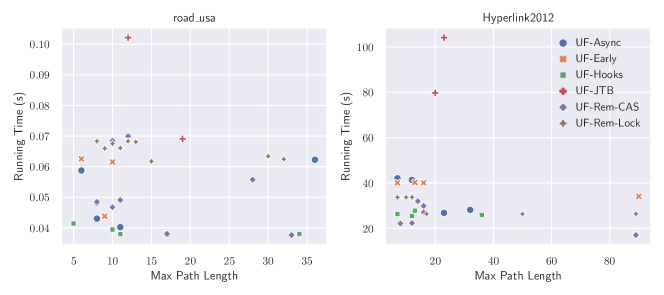
Figure 9. Plot of the Max Path Length encountered during algorithm execution vs. running time in seconds for the road_usa and Hyperlink2012 graphs.

Max Path Length (MPL). Figure 9 plots the Max Path Length statistic vs. the total running time for different union-find variants on the road_usa and Hyperlink2012 graphs, which are the smallest and largest graphs used in our evaluation (the plots for other graphs are elided in the interest of space; we note that they are very similar). We observed that this value is consistently small across all executions for both the smallest and largest graphs we test on, reaching a maximum of 36 on the road_usa graph, and a maximum of less than 100 on the Hyperlink2012 graph. Perhaps surprisingly, this quantity does not seem to be correlated with the running time—on the Hyperlink2012 graph the $\mathsf{UF\mathchar 45\relax Rem\mathchar 45\relax CAS}$ implementation has one of the largest Max Path Lengths, but still achieves the lowest running time in this setting.

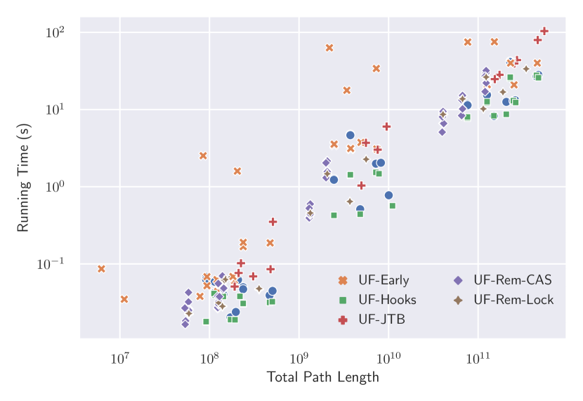
Figure 10. Plot of the Total Path Length traversed during algorithm execution (log-scale) vs. running time in seconds (log-scale) for all union-find experiments on all of our inputs.

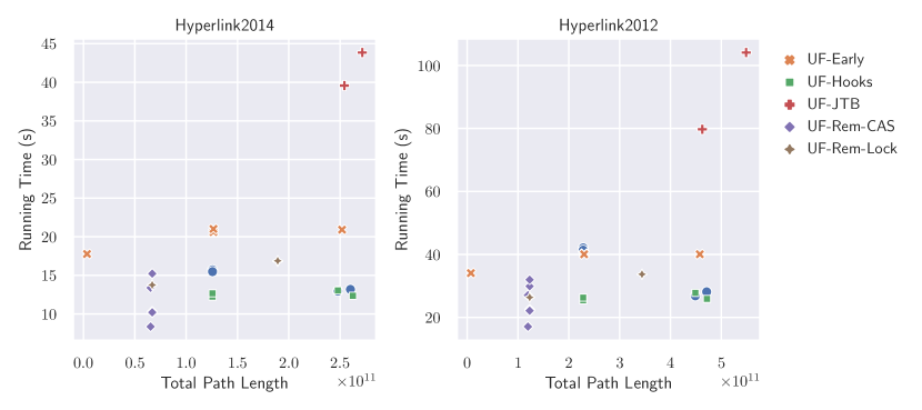
(a) Plot of the Total Path Length traversed during algorithm execution (log-scale) vs. running time in seconds (log-scale) for all union-find experiments on the Hyperlink2014 and Hyperlink2012 graphs.

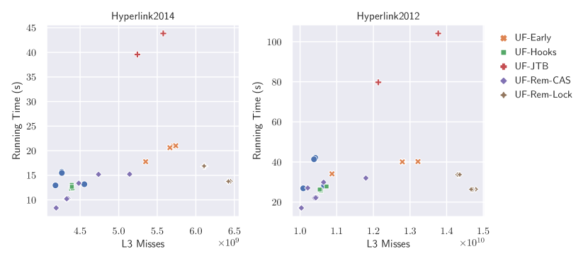
(b) Plot of the number of LLC misses during algorithm execution vs. running time in seconds for all union-find experiments on the Hyperlink2014 and Hyperlink2012 graphs.

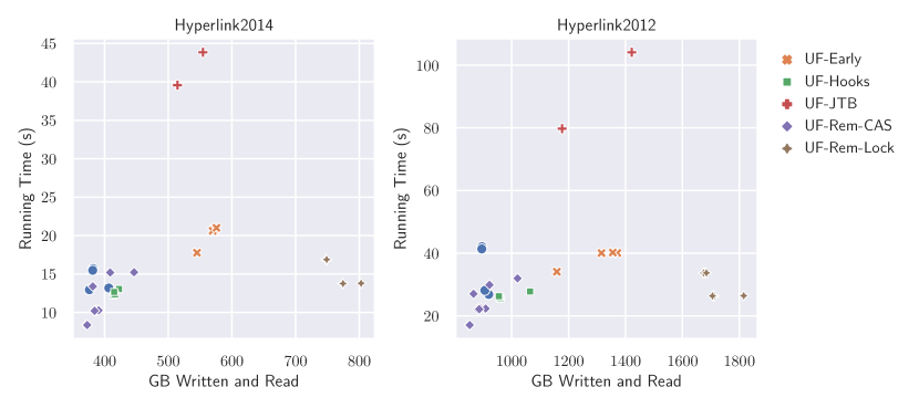
(c) Plot of the total GB written and read during execution vs. running time in seconds for all union-find experiments on the Hyperlink2014 and Hyperlink2012 graphs.

Figure 11. Performance statistics for the Hyperlink2014 and Hyperlink2012 graphs.

Total Path Length (TPL). Figure 10 plots the Total Path Length (TPL) statistic vs. the total running time across all graphs for different union-find variants (both axes are shown in log-scale). The plot shows that the TPL is highly relevant for predicting the running time—the TPL has a Pearson correlation coefficient of 0.738 with the running time (the MPL has a much weaker coefficient of 0.344). Figure 11(a) plots the same statistic for the Hyperlink2014 and Hyperlink2012 graphs, where we see a similar trend. The poor performance of the $\mathsf{UF\mathchar 45\relax JTB}$ algorithms under both find configurations is explained largely by the large total path lengths traversed by these algorithms (the algorithm with larger TPL and running time was always for the $\mathsf{FindNaive}$ implementation). We note that the $\mathsf{UF\mathchar 45\relax Early}$ algorithm exhibits a single data point which experiences significantly lower TPL than any of the other algorithms. This data point is for the version of the $\mathsf{UF\mathchar 45\relax Early}$ algorithm combined with the $\mathsf{FindNaive}$ strategy. Since the algorithm does not perform any finds, the only contribution to the path length is from the path length traversed by the $\mathsf{Union}$ method. Despite this fact, it is interesting that the $\mathsf{UF\mathchar 45\relax Early}$ code with the $\mathsf{FindNaive}$ option incurs such a low TPL. We note that $\mathsf{FindNaive}$ is always the fastest option for this algorithm.

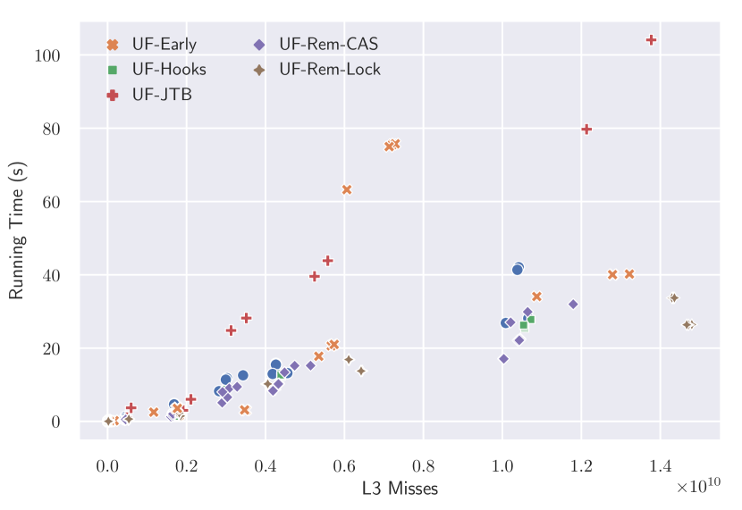
Figure 12. Plot of the number of LLC misses incurred during algorithm execution vs. running time in seconds for all union-find experiments on all of our inputs.

LLC Misses. In Figure 12, we plot the number of LLC misses vs. running time across all graphs. Figure 11(b) plots the same quantities for the Hyperlink2014 and Hyperlink2012 graphs. We see that the $\mathsf{UF\mathchar 45\relax Early}$ implementations, which perform poorly on the Hyperlink2014 graph incur a large number of LLC misses. The Pearson correlation coefficient between the number of LLC misses and the overall running time is 0.797 across all graphs, which is comparable with the correlation between the TPL and the running time. Lastly, we observe that the fastest algorithms incur the fewest number of LLC misses, with $\mathsf{UF\mathchar 45\relax Rem\mathchar 45\relax CAS}$ with the $\mathsf{FindAtomicSplit}$ option achieving the point in the bottom left corner of the plot for the Hyperlink graphs.

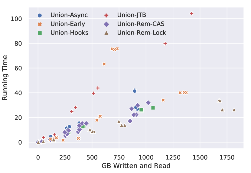
Figure 13. Plot of the total number of bytes written and read (in GB) during algorithm execution vs. running time for all union-find experiments on all of our inputs.

Total Bytes Written/Read. In Figure 13, we plot the total gigabytes written to and read from the memory controller vs. running time across all graphs. Figure 11(c) plots the same quantities for the Hyperlink2014 and Hyperlink2012 graphs. As one might expect, the trends appear to be similar to the number of LLC misses. Perhaps surprisingly, although the $\mathsf{UF\mathchar 45\relax Rem\mathchar 45\relax Lock}$ requires the largest amount of memory traffic, these algorithms are much faster than algorithms that read and write fewer bytes across the memory controllers ($\mathsf{UF\mathchar 45\relax Early}$ and $\mathsf{UF\mathchar 45\relax JTB}$). This quantity has a Pearson correlation coefficient with the running time of 0.774, which is similar to that of the LLC misses statistic. Finally, we observe that the $\mathsf{UF\mathchar 45\relax Rem\mathchar 45\relax CAS}$ and $\mathsf{UF\mathchar 45\relax Async}$ algorithms require reading and writing very little data.

C.1.1. Liu-Tarjan Algorithms

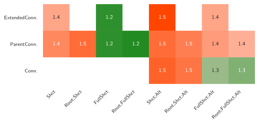
Figure 14. Relative performance of different Liu-Tarjan implementations on graphs used in our evaluation of ConnectIt in the No Sampling setting.

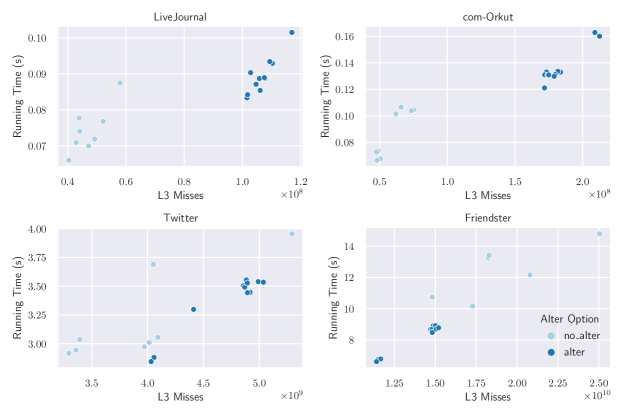
Figure 15. Plot of the number of LLC misses for each algorithm execution vs. running time in seconds for the LiveJournal, com-Orkut, Twitter, and Friendster graphs.

Figure 14 shows the relative performance of different Liu-Tarjan implementations from ConnectIt in the No Sampling setting. These results are averaged across all graphs used in our evaluation, and are computed the same way as in our union-find evaluation previously.

We observed that the four fastest Liu-Tarjan variants in this setting are the new variants we implemented that perform a $\mathsf{FullShortcut}$, namely $\mathsf{PUF}$, $\mathsf{EUF}$, $\mathsf{PRF}$, and $\mathsf{CRFA}$. The remaining methods achieve between 1.3x–1.5x slowdown on average across all graphs, with the slowest algorithms on average being those using the $\mathsf{Alter}$ method.

Figure 15 analyzes how the number of LLC misses affects the running time. We see that the algorithm performance of the Liu-Tarjan variants is significantly determined by the number of LLC misses (the Pearson correlation coefficient is 0.982). We note that the algorithms using the $\mathsf{Alter}$ method are sometimes the fastest Liu-Tarjan variants, which can be seen in Figure 15.

C.2. Parallel Connectivity with Sampling

This section reports additional results, and performance analyses about ConnectIt in the setting where sampling is performed. In particular, we evaluate how ConnectIt algorithms perform when combined with the $k$-out Sampling, BFS Sampling, and LDD Sampling strategies, and discuss the speedups of the sampling-based algorithms compared to the performance numbers without sampling presented in Section 4.1.

ConnectIt Using $k$-out Sampling. The second group of rows in Table 3 shows the performance of ConnectIt algorithms using the $k$-out Sampling scheme on our graph inputs. We observe that the performance of ConnectIt algorithms combined with $k$-out Sampling is consistently fast, and produces the fastest overall algorithm on almost half of our graph inputs (across both small and large graphs). Like in the no sampling setting, the union-find algorithms achieve very high performance, with $\mathsf{UF\mathchar 45\relax Async}$ and $\mathsf{UF\mathchar 45\relax Rem\mathchar 45\relax CAS}$ achieving similar performance (their running times are within a few percent of each other on all of the graphs in this setting). Unlike in the no sampling setting, the performance of other union-find variants is very close to that of the fastest union-find variants, with the slowest overall variant on average being $\mathsf{UF\mathchar 45\relax Rem\mathchar 45\relax Lock}$. On average, the union-find implementations achieve a 2.11x speedup over the fastest connectivity implementations without sampling, with the highest average speedup obtained by $\mathsf{UF\mathchar 45\relax Rem\mathchar 45\relax CAS}$ (2.25x faster than the fastest algorithms without sampling, on average). Our Liu-Tarjan, Shiloach-Vishkin, and label propagation algorithms also achieve high performance when compared with the fastest algorithms for each graph. Liu-Tarjan achieves 1.71x average speedup over the fastest algorithm in the no sampling setting, Shiloach-Vishkin achieves 1.53x average speedup, and label propagation achieves 1.68x average speedup. These results indicate that these algorithms compose efficiently with the $k$-out Sampling scheme.

Across all of our graphs, the one exception where $k$-out Sampling does not provide significant speedups is for the road_usa graph. The main reason is that the road_usa graph has very low average degree, with most vertices having between 2–5 edges. Therefore, the cost of simply going over this small set of edges twice during two-phase execution outweighs the additional benefit provided by sampling, since we almost finish computing connectivity after applying $k$-out Sampling (see Section C.5 for more experimental analysis of $k$-out Sampling on this graph).

Next, we compare the effectiveness of $k$-out Sampling compared with the fastest results obtained by any combination of sampling and finish methods in the ConnectIt framework. We can see from Table 3 that the $\mathsf{UF\mathchar 45\relax Rem\mathchar 45\relax CAS}$ algorithm achieves the most consistent performance relative to the fastest algorithms, being at most 27% slower than the fastest implementation for all graphs, and within 14% on average. $\mathsf{UF\mathchar 45\relax Async}$ and $\mathsf{UF\mathchar 45\relax Hooks}$ are similarly competitive, being at most 30% and 31% slower, and within 19% and 18% of the fastest on average, respectively. We conclude that applying one of these three union-find algorithms in addition to $k$-out Sampling results in consistent high performance.

To summarize, we find that $k$-out Sampling is an effective and robust sampling scheme that consistently works across a variety of different graph types, and algorithm types (union-find variants, Liu-Tarjan variants, and Shiloach-Vishkin) to produce algorithms that are within 1.12x on average of the fastest running times obtained by any algorithm in our framework. Finally, for the Hyperlink2012 graph, the largest publicly-available real-world graph, the $\mathsf{UF\mathchar 45\relax Rem\mathchar 45\relax CAS}$ algorithm combined with $k$-out Sampling achieves the fastest time out of all algorithm combinations in our framework, running in 8.2 seconds in total. This is a 3.14x improvement over the fastest known result for this graph, previously achieved by the Graph Based Benchmark Suite (Dhulipala et al., 2018) using the work-efficient connectivity algorithm by Shun et al. (Shun et al., 2014), and is competitive with two empirical lower-bounds on the performance of any connectivity algorithm (analyzed in Section C.5.1).

Performance Using BFS Sampling. The third group of rows in Table 3 show the performance of ConnectIt algorithms using the BFS Sampling scheme on our graph inputs. We can immediately see that the performance of this method depends significantly on the diameter of the input graph (listed in Table 2) as the number of rounds in parallel BFS is proportional to the diameter—for example, the performance of these methods on the road_usa graph is significantly worse than the unsampled running times (roughly 60–70x slower). One interesting exception is for label propagation, where the algorithm is 5.1x faster than the unsampled version, since the label propagation algorithm can avoid processing the high-diameter component identified by the BFS.

The performance on the remaining graphs is highly competitive: the fastest running time using BFS Sampling achieves between 1.2–4.9x speedup over the fastest running time without sampling, and 2.5x speedup on average. Like with $k$-out Sampling, the fastest running times using BFS Sampling are obtained using union-find variants, with $\mathsf{UF\mathchar 45\relax Rem\mathchar 45\relax CAS}$ running within 3% of the fastest variant using BFS Sampling. $\mathsf{UF\mathchar 45\relax Async}$ and $\mathsf{UF\mathchar 45\relax Hooks}$ are similarly competitive, running between 1.1–4.7x faster and 1.1–4.8x faster than the fastest algorithm without sampling (both achieve 2.4x speedup on average). Finally, we observe that for the three largest graphs, $\mathsf{UF\mathchar 45\relax Rem\mathchar 45\relax CAS}$ consistently achieves the fastest performance out of all variants using BFS Sampling, with BFS Sampling achieving the fastest overall running time for ConnectIt on the Hyperlink2014 graph.

Our Liu-Tarjan, Shiloach-Vishkin, and label propagation algorithms compose efficiently with BFS Sampling, achieving significant speedups over the versions of these algorithms that do not use sampling. On graphs excluding road_usa (where as discussed, BFS Sampling performs poorly), the Liu-Tarjan algorithms achieve between 4.4–28x speedup over the unsampled versions, achieving 12.3x speedup over the unsampled versions on average. Our Shiloach-Vishkin algorithm also achieves strong speedups over the unsampled versions, achieving between 3.87–12.4x speedup, and 7.58x speedup on average. Our label propagation algorithm achieves between 3.41–13.1x speedup over the unsampled label propagation algorithm, and achieves 7x speedup on average.

To summarize, we find that BFS Sampling is a robust sampling strategy that achieves very high performance when combined with our ConnectIt algorithms on low-diameter graphs exhibiting a massive connected component, such as social networks and Web graphs. On high-diameter graphs such as road networks, the performance results suggest that a different sampling scheme, such as $k$-out Sampling would be a better choice, unless the label propagation algorithm is used in which case BFS Sampling is a good choice (the main source of performance improvement for label propagation is having the BFS fully cover the largest component, since the BFS can be accelerated using direction-optimization (Beamer et al., 2012)).

Performance Using LDD Sampling. Finally, we consider the performance of ConnectIt algorithms using the LDD Sampling scheme on our graph inputs (the fourth group of rows in Table 3). First, we consider the high-diameter road_usa graph. Compared to BFS Sampling, the performance numbers using LDD Sampling are significantly better (between 22–25x), except for label propagation where the time using LDD Sampling is 5.5x slower since the massive high-diameter component is still slowly traversed by a large number of costly iterations, even after applying LDD Sampling. The reason for the improvement on other algorithms is since LDD Sampling only requires a few rounds to compute an LDD, whereas a BFS on this network requires thousands of rounds to traverse the high-diameter component in this graph.

Focusing now on low-diameter graphs, the performance of LDD Sampling achieves significant speedups over the ConnectIt algorithms in the no sampling setting. Our $\mathsf{UF\mathchar 45\relax Rem\mathchar 45\relax CAS}$ implementation achieves between 0.98–4.67x speedup over the fastest connectivity implementation in the no sampling setting, and 2.3x speedup on average. $\mathsf{UF\mathchar 45\relax Async}$ and $\mathsf{UF\mathchar 45\relax Hooks}$ also achieve high performance, achieving between 0.96–4.6x and 0.95–4.5x speedup (2.34x and 2.28x speedup on average), respectively. The remaining union-find implementations also achieve high performance under this scheme. Overall, we see that $\mathsf{UF\mathchar 45\relax Rem\mathchar 45\relax CAS}$ is a robust choice in this setting, and is either the fastest implementation, or within 30% of the fastest across all low-diameter graphs. On the three largest graphs, $\mathsf{UF\mathchar 45\relax Rem\mathchar 45\relax CAS}$ is either the fastest algorithm, or within 22% of the fastest running time, and for the largest graph, this algorithm combined with LDD Sampling is within 1% of the fastest running time.

Our Liu-Tarjan, Shiloach-Vishkin, and label propagation algorithms achieve good speedups over the unsampled versions on graphs other than road_usa. The Liu-Tarjan algorithms achieve between 3.5–21.4x speedup over these algorithms in the unsampled versions, and 10x speedup on average. The Shiloach-Vishkin implementation achieves between 3.1–27.3x speedup over the unsampled versions, and 11.6x speedup on average. Finally, the label propagation implementation also achieves good speedup, ranging from 2.1–9.7x speedup, and 5.7x speedup on average.

To summarize, we find that LDD Sampling offers a more robust sampling mechanism compared with BFS Sampling with performance that achieves significant speedups over the ConnectIt algorithms that do not use sampling. Furthermore, its performance is not overly degraded on high-diameter networks, and achieves excellent performance on low-diameter social networks and Web graphs. We perform a thorough analysis of the parameters to the LDD Sampling scheme in Section C.5.

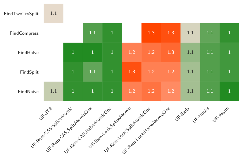
Figure 16. Relative performance of union-find implementations, averaged across all inputs with $k$-out Sampling.

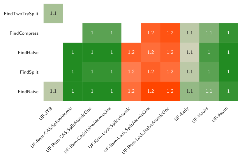
Figure 17. Relative performance of union-find implementations, averaged across all inputs with BFS Sampling.

Union-Find Performance using Sampling. Figures 16, 17, and 18 show heatmaps of the relative performance of different union-find variants when using $k$-out Sampling, BFS Sampling, and LDD Sampling, respectively. Like Figure 3, the running times are aggregated across all of our graph inputs. Unlike Figure 3, the relative running times of each algorithm are significantly closer together for all three sampling schemes, ranging from 1–1.3x slower than the fastest union-find variant on average for $k$-out Sampling, 1–1.2x for BFS Sampling, and 1–1.3x for BFS Sampling. As mentioned previously, the fastest union-find variants are just 1.12x slower on average than the fastest ConnectIt algorithm across all sampling schemes. Therefore, we conclude that applying any union-find variant in conjunction with our sampling schemes results in high performance across all of our graph inputs.

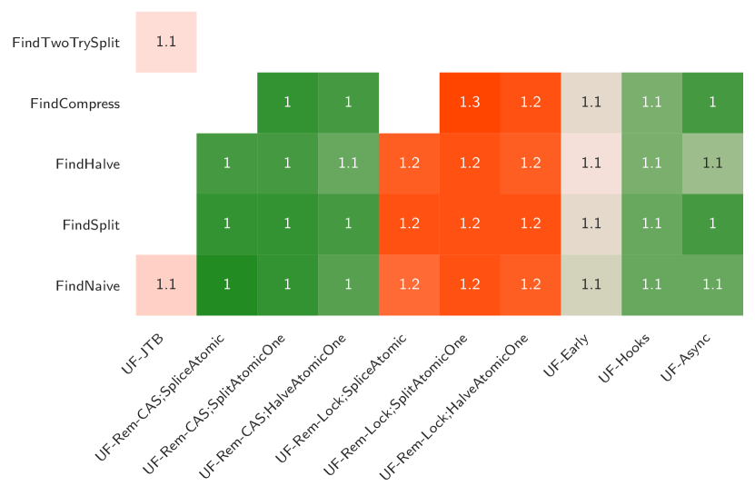
Figure 18. Relative performance of union-find implementations, averaged across all inputs with LDD Sampling.

In summary, all three schemes result in meaningful performance improvements over the unsampled versions, and significantly outperform existing state-of-the-art connectivity results using ConnectIt algorithms.

C.3. ConnectIt vs. State-of-the-Art

In this section, we provide a comparison between ConnectIt and a set of state-of-the-art publicly-available connectivity implementations. The results we analyze can be found in Table 3.

Comparison with BFSCC (Shun and Blelloch, 2014). First, we observe that the BFSCC algorithm has highly variable performance that depends on the input graph diameter. In the no sampling setting for ConnectIt, it ranges from being 92x slower than the fastest ConnectIt algorithm for the road_usa graph, to up to 1.81x and 1.86x faster for the com-Orkut and Twitter graphs, respectively. Compared to ConnectIt algorithms using sampling on instances other than the road_usa graph, where it performs understandably poorly, our implementations are still always faster, ranging from between 1.22–21.7x faster, and 6.46x faster on average.

Comparison with Shun et al. (Shun et al., 2014). We observe that the provably work-efficient LDD-based algorithm from Shun et al. (Shun et al., 2014) achieves more consistent performance across all graphs, including both low and high-diameter networks. Our implementations without sampling are between 1.45–19.4x faster, and 5.6x faster on average. Our implementations with sampling are between 3.1–27.5x faster, and 9.3x faster on average. We note that prior to this paper, this algorithm, implemented as part of the Graph Based Benchmark Suite (GBBS) was the fastest reported running time for the Hyperlink2012 graph, running in 25 seconds (Dhulipala et al., 2018). The fastest ConnectIt algorithm, $\mathsf{UF\mathchar 45\relax Rem\mathchar 45\relax CAS}$ with $\mathsf{SplitAtomicOne}$ improves on this result, even without using any sampling, running in just under 14 seconds.

Comparison with MultiStep (Slota et al., 2014). The MultiStep method implements a hybrid scheme that performs the BFS Sampling scheme combined with label propagation. The MultiStep algorithm performs $O(\mathsf{diam}(G)m+n)$ work in the worst case, and requires $O(\mathsf{diam}(G)\log n)$ depth, where $\mathsf{diam}(G)$ is the graph diameter. The performance of the algorithm is highly variable, especially on high-diameter graphs like road_usa, where it is 2.2x slower than our label propagation implementation. Compared with the fastest ConnectIt implementation without sampling, our implementations are significantly faster, even without sampling. Our codes are between 1.95–21.4x faster across all low-diameter graphs, and 10.1x faster on average. Compared with the fastest ConnectIt implementation with sampling, our codes are between 9.6–30.3x faster across all low-diameter graphs, and 18.6x faster on average. Their code performs significantly worse than ours on road_usa, running 1,057x slower than our fastest code. We note that their algorithm was unable to successfully run on the Twitter graph. Compared to the Slota et al. implementation, our implementation of the MultiStep approach (BFS Sampling combined with label propagation) is between 3.9–22x faster than their implementation, and 12.8x faster on average. The MultiStep code implements the direction-optimization, but we observed that their BFS performance is significantly slower than BFS performance in ConnectIt, which could be due to a cache-optimized version of the edge traversal from the Graph Based Benchmark Suite used in our implementation.

Comparison with Galois (Nguyen et al., 2013). The connectivity algorithm implemented in Galois uses label propagation in conjunction with a priority-based asynchronous scheduler (Nguyen et al., 2013). The algorithm is not work-efficient, and we are not aware of any theoretical upper-bounds on its work when using Galois’ priority-based scheduler. Excluding the road_usa graph where their code performs very poorly using label propagation, our codes without sampling are between 1.78–3.69x faster than theirs (2.36x faster on average), and our codes using sampling are between 2.84–12.6x faster than theirs (7.27x faster on average). Our codes are 2.17x faster than their Async algorithm on the road_usa graph (we tried other implementations from Galois and report times for the fastest one, since their label propagation implementation performed poorly on this graph). Finally, their slow performance on the Twitter graph is likely due to the fact that the Galois implementation requires multiple rounds, where a large fraction of the vertices are active when performing label propagation.

Comparison with Patwary et al. (Patwary et al., 2012b). The connectivity algorithm by Patwary et al. is a concurrent version of Rem’s algorithm. The algorithm is the same as the $\mathsf{UF\mathchar 45\relax Rem\mathchar 45\relax Lock}$ implementation in our framework. However, we find that our implementations are significantly faster than theirs, and that both of our implementations of Rem’s algorithms are competitive with, and often outperform theirs. Our fastest implementations without sampling achieve between 1.27–2.87x speedup over their implementation (1.99x speedup on average), and our fastest implementations with sampling achieve between 2.43–6.28x speedup over their implementation (4.4x speedup on average). We note that they also provide a lock-free version of Rem’s algorithm, but we observed that this algorithm does not always produce correct answers, and thus do not report results for it.

Comparison with GAPBS (Beamer et al., 2015). Finally, we compare ConnectIt with the Shiloach-Vishkin and Afforest implementations from the GAP Benchmark Suite (GAPBS). The Shiloach-Vishkin implementation from GAPBS suffers from an implementation issue that can cause it to perform $O(mn)$ work and $O(n)$ depth in the worst case (under an adversarial scheduler), but we note that this behavior does not seem to arise in practice. The Afforest implementation is implemented jointly with the authors of the Afforest paper by Sutton et al. (Sutton et al., 2018), and was always faster than the original Afforest implementation (Sutton et al., 2018). Our fastest implementations significantly outperform their Shiloach-Vishkin implementation. Our fastest implementations without sampling are between 3.67–17.9x faster (9.55x faster on average), and our fastest implementations with sampling are between 3.67–61.2x faster (27.1x faster on average). We observe that the Afforest algorithm is sometimes faster than our algorithms without sampling (note that Afforest does perform sampling). Our fastest implementations without sampling are between 0.33–4.17x faster than their Afforest implementation (2.08x faster on average). Our fastest implementations with sampling are between 1.53–8.55x faster than their Afforest implementation (3.9x faster on average). We perform an in-depth evaluation of the Afforest sampling scheme in Section C.5.

C.4. Streaming Parallel Graph Connectivity

In this appendix, we provide deferred experimental results on our ConnectIt streaming algorithms. We provide more experimental results showing tradeoffs between batch size and throughput, and addition latency plots.

Additional Observations about Throughput Experiments. We observe that the throughput of all algorithms, even on the smallest graph that we consider is at least hundreds of millions of updates per second for all graphs. In general, the throughput appears to be higher for larger graphs, although some graphs, such as com-Orkut have very high throughput despite being quite small, which could be due to cache effects, since the vertex data fits within LLC. Another source of high performance is that the updates within a batch are left unpermuted in this experiment, and are ordered lexicographically. This ordering provides good data locality when performing work, since the consecutive edges that are applied are likely to contain vertices whose IDs are close together in the vertex ordering.

We ran an experiment to measure the effect of the edge ordering on throughput across different input graphs and found that the performance difference between the two methods scales almost linearly with the number of LLC cache misses incurred by the algorithm. For example, for the Twitter graph, applying the edges of the graph in a single batch for the $\mathsf{UF\mathchar 45\relax Rem\mathchar 45\relax CAS}$ algorithm with $\mathsf{SplitAtomicOne}$ without and with permuting the batch results in 3.85 billion and 2.23 billion edges per second, respectively, or a 1.72x higher throughput in the unpermuted setting. The number of LLC misses measured in these settings is 1.10 billion and 2.05 billion, respectively, which is 1.8x fewer misses in the unpermuted setting. The trend is similar for other graphs, with the performance gap explained by the larger number of cache misses in the permuted setting. We feel that enforcing that batches are permuted is somewhat unrealistic, since our expectation is that real-world data streams possess a large degree of locality (intuitively many of the same vertices are updated, and updates to the same vertex are likely to occur in close succession).

Throughput vs. Batch Size. Figure 19 shows the throughput obtained by our algorithms as a function of the batch size for a subset of our input graphs (the trends for graphs not shown in the figure are very similar). We observe that all ConnectIt algorithms achieve consistently high throughput on very small to very large batch sizes. Our fastest union-find algorithms achieve a throughput of over 10 million updates per second at a batch size of 100, and exceed 100 million updates per second for batches of size 1,000 on all graphs.

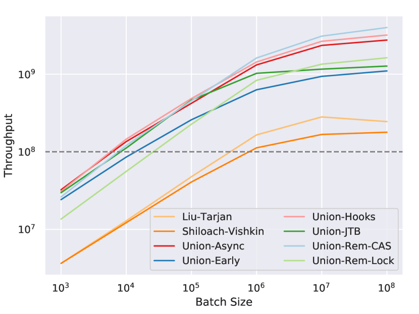
(a) Throughput vs. batch-size for road_usa

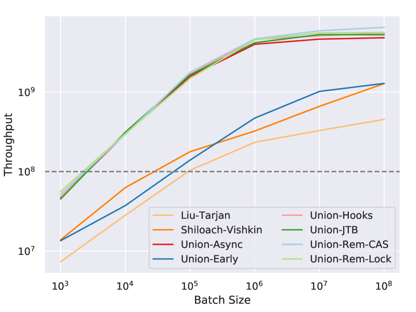
(b) Throughput vs. batch-size for Orkut

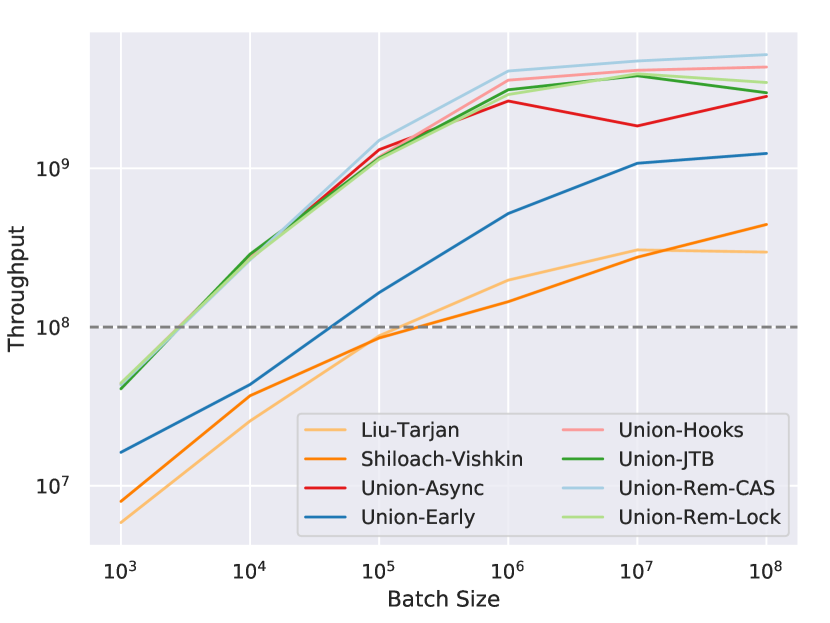
(c) Throughput vs. batch-size for LiveJournal

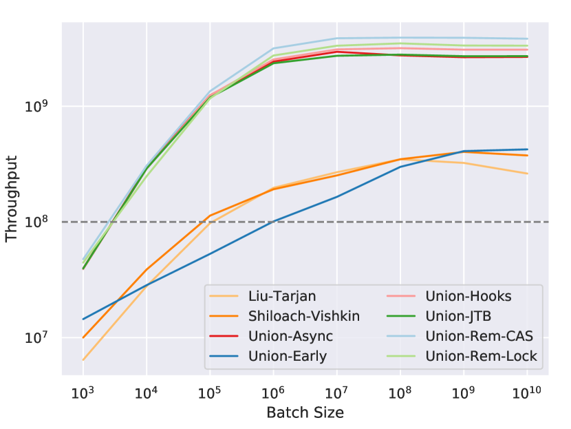
(d) Throughput vs. batch-size for Twitter

Figure 19. Throughput vs. batch size of different union-find implementations on different graphs. The experiment is run on a 72-core machine with 2-way hyper-threading enabled.

Mixed Inserts and Queries Throughput. In these experiments we study how the ratio of insertions to queries affects the overall throughput. We use the $\mathsf{UF\mathchar 45\relax Rem\mathchar 45\relax CAS}$ algorithm as a case study for this experiment, and evaluate the performance of different variants of this algorithm, varying the ratio of insertions to updates. To generate an update stream with an insert-to-query ratio of $x$, we generate $1/x$ many queries on random pairs of vertices, and create a batch permuting the original updates and queries together. Another alternate experiment would be to fix a particular batch size, and then vary the ratio of queries to updates. We tried this strategy but observed that this has the undesirable effect of varying the number of connected components, which affects both query and update performance and thus makes it difficult to interpret the results. Instead, we choose to fix the updates, and generate random pairs of vertices to use as queries. Unlike the experiments in the previous section, we randomly permute the batch so as to accurately reflect the cost of the $\mathsf{UF\mathchar 45\relax Rem\mathchar 45\relax CAS}$ variants which must reorder a batch for correctness.

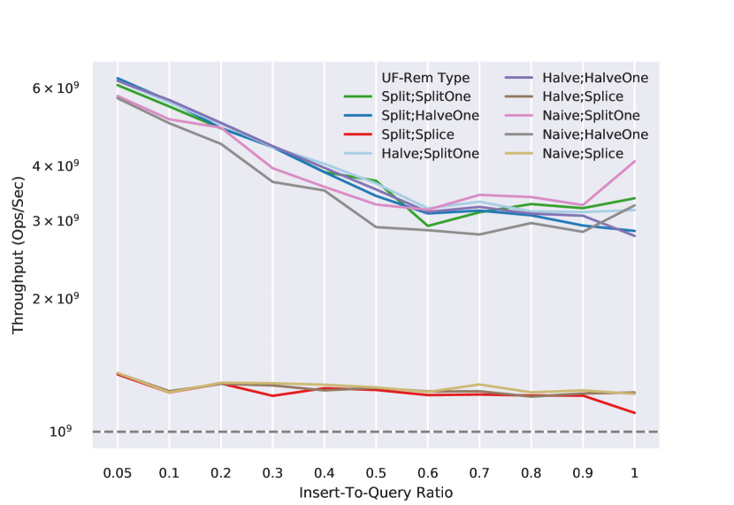
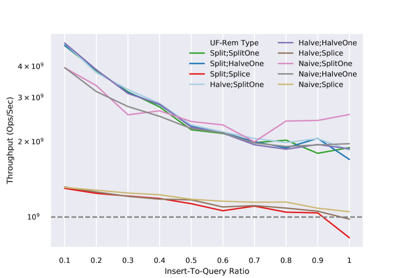
Figure 20. Throughput of different $\mathsf{UF\mathchar 45\relax Rem\mathchar 45\relax CAS}$ implementations on the com-Orkut and LiveJournal graphs, plotted against the ratio of insertions to queries in a batch. The experiment is run on a 72-core machine with 2-way hyper-threading enabled.

Figure 20 shows the result of this experiment on com-Orkut and LiveJournal graphs (the results for other graphs are similar). We observe that the throughput of the algorithms is higher when the ratio between the inserts-to-queries is small, and gradually drops as the ratio approaches $1$. We also observe that the ordering of the algorithms (the relative throughputs) changes as the ratio of inserts-to-queries changes. When there are very few inserts and mostly queries, the fastest algorithms are those that perform additional compression within the query, since queries can help subsequent queries save work by compressing the paths traversed in the union-find trees. On the other hand, when the ratio of inserts-to-queries is large, the algorithms that perform best are those which perform no additional compression during the finds. On both graphs, after a ratio of about 0.6–0.7, the fastest algorithm is the variant which performs no additional compression on a find, and uses the $\mathsf{SplitAtomicOne}$ option (like in the static setting).

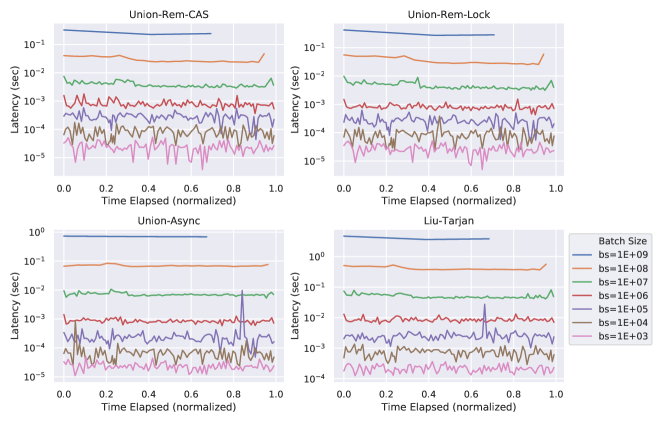
Figure 21. Latency of batch operations (seconds) plotted for varying batch sizes for the $\mathsf{UF\mathchar 45\relax Rem\mathchar 45\relax CAS}$, $\mathsf{UF\mathchar 45\relax Rem\mathchar 45\relax Lock}$, $\mathsf{UF\mathchar 45\relax Async}$, and $\mathsf{Liu\mathchar 45\relax Tarjan}$ algorithms on the Hyperlink2012 graph. The running time of each operation sequence is normalized by the duration of the experiment at that batch size. The $y$-axis is in log-scale. All experiments are run on a 72-core machine with 2-way hyper-threading enabled.

Additional Latency Plots. Figure 21 shows the latency of different ConnectIt implementations while processing an update-only sequence containing a 10% sample of the Hyperlink2012 graph. We observe that the latency for all of our algorithms is highly consistent, with the median time per batch for different batch sizes always being within 1–2% of the average batch time across all algorithms and graphs. The update time, which is plotted in log-scale, grows linearly with the batch size which is also linearly increasing in log-scale. Since the total time taken to process the graph at different batch sizes is different, we rescale the $x$-axis for each experiment to lie in the range $[0,1)$, and subsample the streams to plot a manageable number of operations. We plot the operations as occurring at their start time.

C.5. Sampling Evaluation

We now discuss the empirical performance of the sampling methods presented in this paper. We focus on analyzing (i) the running time of each sampling method; (ii) the fraction of the vertices covered by the largest component the sampling method identifies; and (iii) the number of inter-component edges remaining after running the sampling method.

Graph	$\mathsf{BFS}$ (s)	$\mathsf{BFS}$ Cov.	$\mathsf{BFS}$ IC.	$\mathsf{LDD}$ (s)	$\mathsf{LDD}$ Cov.	$\mathsf{LDD}$ IC.
RU	2.67	100%	0%	0.0743	100%	0%
LJ	0.0109	99.9%	0.0129%	0.0136	99.9%	0.0129%,
CO	0.00909	100%	0%	0.00823	100%	0%
TW	0.0868	100%	0%	0.117	100%	0%
FR	0.330	100%	0%	0.3266	29.0%	43.9%
CW	2.04	97.6%	0.161%	1.523	97.6	0.161%
HL14	2.49	91.4%	0.560%	3.101	91.4%,	0.530%,
HL12	8.42	93.9%	0.538%	7.586	93.9%	0.483%,

Table 6. Performance of the BFS Sampling and LDD Sampling schemes on graphs used in our experiments. The Cov. columns report the percentage of vertices captured in the most frequent component captured by the sampling method. The IC. columns report the fraction of inter-component edges remaining after applying the sampling method. All times reported are measured on a 72-core machine (with 2-way hyper-threading enabled).

BFS Sampling and LDD Sampling Performance. We start with the closely related BFS Sampling and LDD Sampling schemes. Table 6 reports the running times and sampling quality of these two schemes. For LDD Sampling, we report the results using the fixed parameters that are used in our experiments ($\beta=0.2$, and setting permuting to $\mathsf{False}$).

Perhaps as expected, the running time of BFS Sampling is high on the high-diameter road_usa graph, although it completely covers this graph achieving 100% coverage, with no inter-component edges remaining. For the remaining graphs, the running times are reasonable, and a BFS from a random source covers a large portion of the graph, leaving just a fraction of a percentage of inter-component edges on four of our graphs.

For LDD Sampling, the performance is quite reasonable, running in close to the running time of a BFS on each of these graphs, ranging from 35.9x faster on road_usa, to at most 1.24x slower on Hyperlink2014. LDD Sampling achieves an average speedup of 5.35x over BFS Sampling, running between 1.39x slower to 1.34x faster, and is within 1% of the running time of BFS Sampling on average on graphs excluding road_usa. Thus, for graphs with low to moderate diameter, the performance of the two schemes is roughly equivalent. Compared to BFS Sampling, LDD Sampling achieves similar coverage of vertices in the most frequent connected component, and also cuts a similar number of inter-component edges, actually cutting 5–11% fewer edges on both the Hyperlink2014 and Hyperlink2012 graphs. However, both schemes already cut fewer than 1% of the edges, and so the difference in quality is very modest.

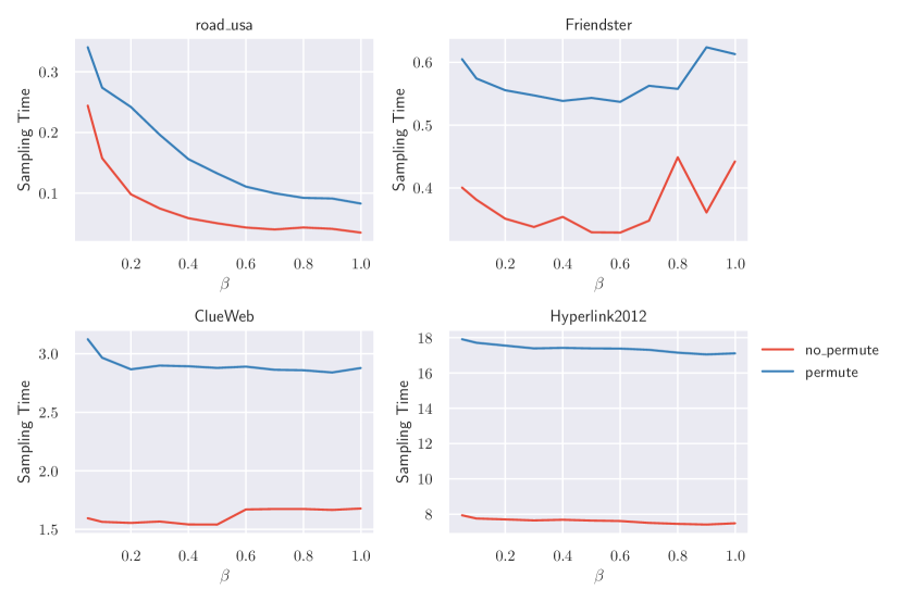
Figure 22. Plot of $\beta$ vs. running time (seconds) when permuting is both enabled and disabled in LDD sampling. Experiments are run on a 72-core machine with 2-way hyper-threading.

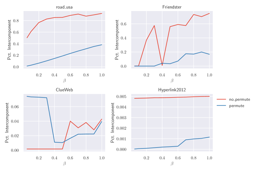
Figure 23. Plot of $\beta$ vs. fraction of inter-component edges remaining after sampling when permuting is both enabled and disabled in LDD sampling.

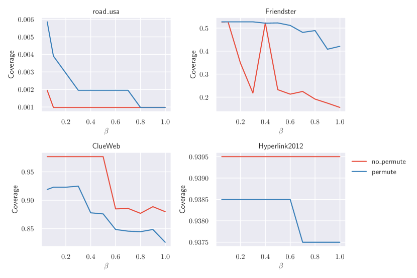
Figure 24. Plot of $\beta$ vs. percentage of vertices covered in the largest component when permuting is both enabled and disabled in LDD sampling.

LDD Sampling Parameters. Next, we study how adjusting the value of $\beta$ and applying a random permutation on the vertex ordering in the LDD algorithm affects both the coverage and number of inter-component edges. In theory, the $\beta$ parameter in LDD Sampling controls both the strong diameter of the components, as well as the number of edges cut in the graph in expectation. In particular, for some $0<\beta<1$, LDD Sampling produces clusters with diameter $O(\log n/\beta)$, and cuts $O(\beta m)$ edges in expectation.

Figure 22 plots the tradeoff between different values of $\beta$ and the overall running time of the algorithm on four of our input graphs, including the high-diameter road_usa graph, the Friendster social network, and the ClueWeb and Hyperlink2012 Web graphs. We see that for road_usa, the running time decreases as a function of $\beta$, which is expected since larger values of $\beta$ produce lower-diameter clusterings which in turn require fewer synchronous rounds to compute. However, higher values of $\beta$ also indicate a larger number of distinct components, since more vertices wake up in early rounds and start their own clusters. This explains why the running time actually increases for large values of $\beta$ on the Friendster graph.

Figure 23 plots the fraction of inter-component edges; letting $I$ be the fraction of inter-component edges, the theory predicts that $I\approx\beta$. This fraction is of interest, since $I$ is a lower-bound on the number of edges that must be processed by our connectivity algorithms, since all edges coming out of the most frequently identified component are skipped. We can see that theory is very useful in predicting the number of inter-component edges—for the road_usa graph, the number of inter-component edges grows linearly with $\beta$ (almost exactly following the line $.4\beta$). We also observe that the number of cut edges is not always monotonically increasing with $\beta$, which can be observed on the ClueWeb graph, although the fraction of cut edges does seem to grow as $\beta$ is increased as a rule of thumb.

Lastly, Figure 24 shows the fraction of vertices covered in the most frequent component identified by LDD Sampling, for different values of $\beta$. We see that the size of this component is extremely small for the road_usa graph (less than 1%), which is consistent with what theory would predict for a high-diameter graph. For lower-diameter graphs, the fraction covered in the most frequent component is much higher, ranging from 80%–98% for the ClueWeb graph and 93%-94% for the Hyperlink2012 graph. Both using a random permutation and using the original vertex ordering perform well, although on the large real-world Web graphs, the original ordering consistently produces a massive component that is 1–5% larger than the one produced by a random permutation of vertices.

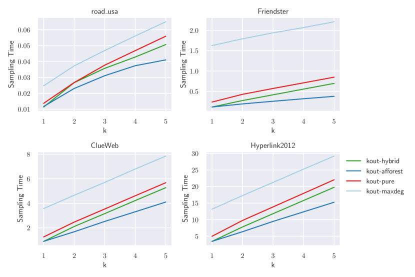
Figure 25. Plot of $k$ vs. running time (seconds) for different variants of $k$-out Sampling. Experiments are run on a 72-core machine with 2-way hyper-threading.

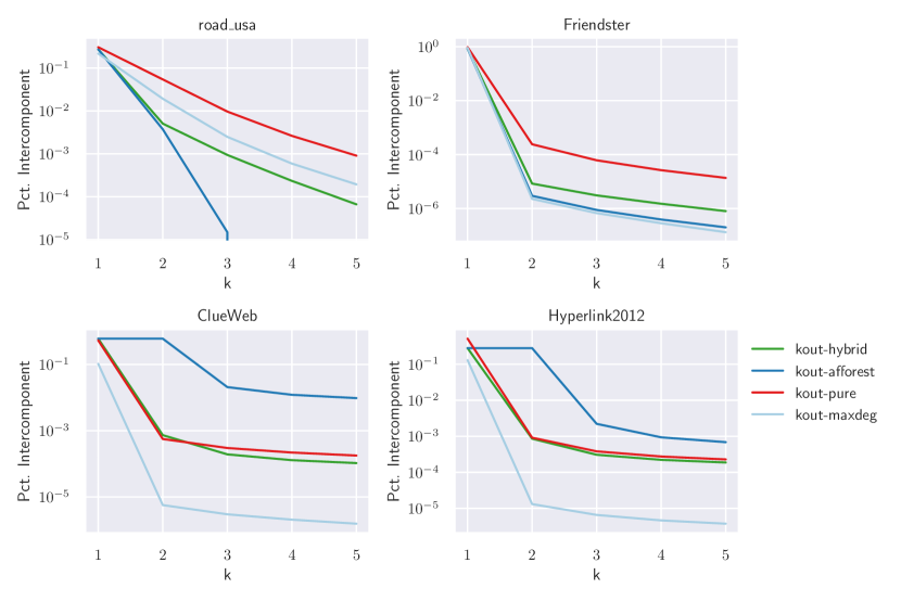
Figure 26. Plot of $k$ vs. fraction of inter-component edges remaining after sampling for different variants of $k$-out Sampling.

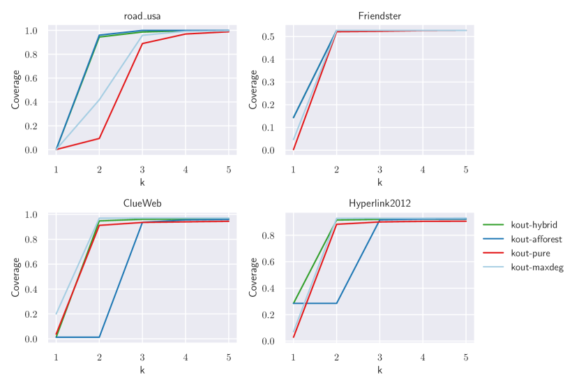
Figure 27. Plot of $k$ vs. percentage of vertices covered in the largest component for different variants of $k$-out Sampling.

$k$-out Sampling. We now turn to $k$-out Sampling, which is particularly interesting due to both its connection with recent fundamental theoretical results (Holm et al., 2019). As described in Section 3.2, given an input $k\geq 1$, the algorithm implemented in this paper selects the first neighbor incident to each vertex, and selects $k-1$ other edges uniformly at random. The sampled components are computed by contracting all selected edges. We use a union-find algorithm to perform the contraction, but note that other min-based algorithms can also be used for this step.

However, there are several other design possibilities and options in this scheme. We explore the following $k$-out algorithm variants in this paper, which differ in how they select edges to use in the $k$-out algorithm (Algorithm 4).

• Afforest ($\mathsf{kout\mathchar 45\relax afforest}$): This scheme proposed by Sutton et al. (Sutton et al., 2018) selects the first $k$ edges incident to each vertex to use.

• Pure Sampling ($\mathsf{kout\mathchar 45\relax pure}$): This scheme proposed by Holm et al. (Holm et al., 2019) selects $k$ edges incident to each vertex uniformly at random to use.

• Hybrid Sampling ($\mathsf{kout\mathchar 45\relax hybrid}$): This scheme selects the first edge incident to each vertex, and $k-1$ edges incident to the vertex uniformly at random to use.

• Max-Degree Sampling ($\mathsf{kout\mathchar 45\relax maxdeg}$): This scheme selects the edge corresponding to the largest degree neighbor incident to each vertex, and $k-1$ edges other incident to the vertex uniformly at random to use.

Both the $\mathsf{kout\mathchar 45\relax hybrid}$ and $\mathsf{kout\mathchar 45\relax maxdeg}$ schemes are new strategies proposed in this paper. We are not aware of any experimental evaluation of the $\mathsf{kout\mathchar 45\relax pure}$ scheme proposed by Holm et al. (Holm et al., 2019) prior to our work. The result Holm et al. provide for $\mathsf{kout\mathchar 45\relax pure}$ is as follows:

Theorem 1.

Let $G$ be an undirected $n$-vertex graph and let $k\geq c\log n$, where $c$ is a sufficiently large constant. Let $G^{\prime}$ be a random $k$-out subgraph of $G$. Then the expected number of edges in $G$ that connect different connected components of $G^{\prime}$ is $O(n/k)$.

$k$-out Sampling Running Time. Figure 25 shows the running times of the different strategies on four of our graph inputs. We observe that the $\mathsf{kout\mathchar 45\relax maxdeg}$ strategy consistently requires the largest running times, since it requires reducing over all edges incident to the vertex, and performing an indirect read on the neighboring endpoint to find the largest degree neighbor. The other schemes all have a similar cost, with $\mathsf{kout\mathchar 45\relax afforest}$ being the fastest across all graphs, and $\mathsf{kout\mathchar 45\relax pure}$ being the second slowest across all graphs. As expected, $\mathsf{kout\mathchar 45\relax hybrid}$’s performance interpolates that of $\mathsf{kout\mathchar 45\relax hybrid}$ and $\mathsf{kout\mathchar 45\relax pure}$, and is equal to the performance of $\mathsf{kout\mathchar 45\relax afforest}$ for $k=1$. This is expected, since the hybrid algorithm is the same as $\mathsf{kout\mathchar 45\relax afforest}$ for $k=1$, and selects $k-1$ random edges, thus approximating the performance of $\mathsf{kout\mathchar 45\relax pure}$ for larger $k$.

$k$-out Sampling Inter-Component Edges. Figure 26 plots the fraction of inter-component edges generated by different variants of the $k$-out Sampling scheme as a function of $k$. We plot the fraction of inter-component edges in log-scale to help interpret the plot. We see that using $k=1$ performs very poorly for all schemes, with the exception of the $\mathsf{kout\mathchar 45\relax maxdeg}$ scheme, where it achieves reasonable performance for the ClueWeb and Hyperlink2012 graphs (both of these graphs are power-law degree distributed, and have several very high degree vertices). The $\mathsf{kout\mathchar 45\relax afforest}$ scheme performs very well on the road_usa graph, probably due to the fact that most vertices in this graph have just a few neighbors—for $k\geq 4$ the $\mathsf{kout\mathchar 45\relax afforest}$ sampling scheme finds all components of this graph and thus the inter-cluster edge percentage is 0 for $k\geq 4$. For the other graphs, the $\mathsf{kout\mathchar 45\relax maxdeg}$ scheme consistently performs best.

The $\mathsf{kout\mathchar 45\relax pure}$ and $\mathsf{kout\mathchar 45\relax hybrid}$ schemes perform similarly, with the $\mathsf{kout\mathchar 45\relax hybrid}$ scheme usually performing slightly better when the $\mathsf{kout\mathchar 45\relax afforest}$ algorithm performs well due to the graph’s vertex ordering. On the other hand, for the ClueWeb and Hyperlink2012 graphs, the $\mathsf{kout\mathchar 45\relax afforest}$ scheme performs quite poorly—these appear to be instances where greedily taking the first $k$ vertices based on the input vertex order results in the graph clustering into local clusters, with many inter-cluster edges between them. The vertex orders of these graphs are based on the lexicographical ordering of pages on the Web, which orders web pages within the same domain consecutively. Therefore, one explanation for this behavior is that the first $k$ edges are all ”inter-domain” edges which result in clusters based on domains being formed by the sampling algorithm.

Graph	$\mathsf{KOut(Hybrid)}$ (s)	$\mathsf{KOut(Hybrid)}$ Cov.	$\mathsf{KOut(Hybrid)}$ IC.
RU	0.0267	94.4%	0.505%
LJ	8.82e-2	99.9%	4.20e-4%
CO	8.574e-2	100%	0%
TW	0.112	99.9%	5.66e-3%
FR	0.274	52.7%	8.39e-4%
CW	2.11	94.8%	0.735%
HL14	3.31	89.9%	0.0323%
HL12	7.79	91.5%	0.0857%

Table 7. Performance of the $k$-out Sampling schemes on graphs used in our experiments. The Cov. column reports the percentage of vertices captured in the most frequent component captured by the sampling method. The IC. column reports the fraction of inter-component edges remaining after applying the sampling method. All times reported are measured on a 72-core machine (with 2-way hyper-threading enabled).

$k$-out Sampling Coverage. Next, Figure 27 plots the fraction of vertices contained in the most frequent component identified by sampling as a function of $k$. The results are similar to those previously analyzed from Figure 26: on some graphs with good vertex orderings (road_usa, Friendster), $\mathsf{kout\mathchar 45\relax afforest}$ achieves excellent performance. However, on other graphs (ClueWeb, Hyperlink2012), $\mathsf{kout\mathchar 45\relax afforest}$ achieves very poor performance due to the ordering containing significant local structure that prevents large components from forming. The $\mathsf{kout\mathchar 45\relax pure}$ algorithm addresses this issue, and achieves consistent performance on all graphs. The $\mathsf{kout\mathchar 45\relax hybrid}$ algorithm further improves the performance of $\mathsf{kout\mathchar 45\relax pure}$, significantly outperforming $\mathsf{kout\mathchar 45\relax afforest}$ on the ClueWeb and Hyperlink2012 graphs for $k=2$, and achieving performance close to $\mathsf{kout\mathchar 45\relax afforest}$ on the other graphs. Table 7 shows the running times, percent coverage, and percent of inter-component edges remaining for the $k$-out Sampling scheme used in our paper ($k=2$ using the $\mathsf{kout\mathchar 45\relax hybrid}$ algorithm).

$k$-out Sampling Summary. Finally, we consider how the performance of these schemes compares with the predictions of the theory. First, we note that the theory rules out the possibility of Theorem 1 holding for $k=1$ (however, it is conjectured to hold for $k\geq 2$). We see that in practice for $k\geq 2$ a huge fraction of the edges become intracluster, with very few remaining inter-cluster edges, and far fewer edges remain than predicted by theory. For example, for the Hyperlink2012 graph, the $\mathsf{kout\mathchar 45\relax pure}$ scheme results in 0.0009149% inter-component edges, or 206M inter-component edges, which is about 1/20th the number of vertices in this graph. Our results suggest that the empirical performance of these schemes is far better than suggested by theory. It would be interesting to explore applying these ideas to speed up connectivity algorithms in other settings, such as practical distributed connectivity implementations, or possibly even in practical dynamic connectivity algorithms.

C.5.1. Comparison with MapEdges and GatherEdges

Next, we compare the cost of our connectivity algorithms with two basic graph processing primitives, MapEdges and GatherEdges. These are primitives that map over all vertices in parallel, and perform a parallel reduction over their incident edges, storing the result in an array proportional to the number of vertices. MapEdges returns a value of $\mathsf{1}$ per edge, which corresponds to computing the degree of each vertex after reading every edge. GatherEdges performs an indirect read into an array at the location corresponding to the neighbor id, and so the performance of this primitive depends on the structure and ordering of the input graph.

Both primitives are useful baselines for understanding the performance of more complex graph algorithms. In particular, MapEdges corresponds to the cost of reading and processing a graph input, and storing some output value for each vertex. GatherEdges serves as a useful practical lower-bound on the performance of graph algorithms that perform indirect accesses over every edge. This is useful for connectivity algorithms, since every connectivity algorithm that always outputs a correct answer (Las Vegas algorithm) must check some connectivity information for both endpoints of an edge, which seems impossible to do without performing an indirect read. All connectivity algorithms in our framework perform an indirect read across every edge to the parent array of the neighboring vertex.

Table 8 shows the running time of the MapEdges and GatherEdges primitives, and the time taken by the fastest connectivity implementation in ConnectIt for that graph. First, we observe that there is an order of magnitude difference in running times between the MapEdges and GatherEdges: GatherEdges is 13.5x slower on average than MapEdges across all inputs. The difference between the two is more noticeable for small graphs, since the sequential reads used in MapEdges are likely to be served by cache. On the other hand, for GatherEdges, even our smallest graph has 23.9M vertices, whose vertex data is already larger than our multicore machine’s LLC, and thus many of the indirect reads across edges will be cache misses.

Graph	MapEdges	GatherEdges	(No Sample)	ConnectIt (Sample)
road_usa	5.54e-3	1.33e-2	2.80e-2	3.77e-2
LiveJournal	1.31e-3	8.59e-3	1.27e-2	8.96e-3
com-Orkut	9.77e-4	1.65e-2	1.91e-2	8.56e-3
Twitter	2.63e-2	0.488	0.316	9.24e-2
Friendster	2.77e-2	1.50	0.902	0.183
ClueWeb	0.790	2.77	4.04	1.69
Hyperlink2014	1.36	4.14	6.64	2.83
Hyperlink2012	2.96	10.4	13.9	8.20

Table 8. 72-core with hyper-threading running times (in seconds) comparing the performance of GatherEdges to the performance of the fastest connectivity implementation in ConnectIt without sampling (No Sample), and with sampling used (Sample).

C.6. Algorithms for Massive Web Graphs

Table 1 in the introduction presents the results of comparing ConnectIt algorithms with these existing state-of-the-art results from different computational paradigms. We can see that in all cases, ConnectIt achieves significant speedup, sometimes ranging on orders of magnitude in terms of raw running time alone. We now provide a detailed breakdown of how ConnectIt algorithms compare with the fastest systems from different categories.

Distributed Memory Systems

There have been various distributed-memory connected components algorithms that report running times for Hyperlink2012, which we compare with here. Slota et al. (Slota et al., 2016) present a distributed-memory connectivity algorithm, and report a running time of 63 seconds for finding the largest connected component on the Hyperlink2012 graph using 8,192 cores (256 nodes each with two 16-core processors) on the Blue Waters supercomputer. Stergiou et al. (Stergiou et al., 2018) describe a distributed-memory connected components algorithm. Using 12,000 cores (1,000 nodes each with two 6-core CPUs) and 128TB of RAM on a proprietary cluster at Yahoo!, they report a running time of 341 seconds for this graph. Dathathri et al. (Dathathri et al., 2018) report a running time of 75.3 seconds for connected components in the D-Galois graph processing system for Hyperlink2012 using 256 nodes (each with a KNL processor with 68 cores and 96GB RAM) on the Stampede KNL Cluster. Very recently, Zhang et al. (Zhang et al., 2020) present a variant of Shiloach-Vishkin for distributed-memory and report a running time of 30 seconds on 262,000 cores of an XC40 supercomputer. Compared with these results, our fastest times are significantly faster.

• Compared to Slota et al. (Slota et al., 2016), our results are 7.68x faster, using a machine with 16x less memory, and 56x fewer hyper-threads. Additionally, our algorithm finds all connected components, whereas their algorithm can only find the largest connected component (this is trivial to do on this graph by running a breadth-first search from a random vertex).

• Compared to Stergiou et al. (Stergiou et al., 2018), our results achieve 41.5x speedup over their result, using 128x less memory, and 166x fewer hyper-threads.

• Compared to the recent results of Dathathri et al. (Dathathri et al., 2018), our results are 9.18x faster. Furthermore, we use 24x less memory, and 483x fewer hyper-threads.

• Compared to the very recent results of Zhang et al. (Zhang et al., 2020), which is the fastest current distributed-memory running time to solve connectivity on this graph, our results are 3.65x faster, using at least 256x less memory (each node on their system has at least 64GB of memory, to up to 256GB of memory, but unfortunately the authors did not report these statistics), and 1,819x fewer hyper-threads.

External Memory Systems

Mosaic (Maass et al., 2017) reports in-memory running times on the Hyperlink2014 graph. Their system is optimized for external memory execution. They solve connected components in 700 seconds on a machine with 24 hyper-threads and 4 Xeon-Phis (244 cores with 4 threads each) for a total of 1,000 hyper-threads, 768GB of RAM, and 6 NVMe SSDs. FlashGraph (Zheng et al., 2015) reports disk-based running times for the Hyperlink2012 graph on a 4-socket, 32-core machine with 512GB of memory and 15 SSDs. On 64 hyper-threads, they solve connected components in 461 seconds.

• Compared with Mosaic, ConnectIt is 247x faster, using 1.3x more memory, but 6.94x fewer hyper-threads. Although the Xeon-Phi chips Mosaic uses are no longer available, from a cost perspective, machines like the one we use in this paper are widely available from existing cloud service providers for a few dollars on the hour, but to the best of our knowledge, one cannot easily rent a machine like the one used in Mosaic.

• Compared with FlashGraph’s result for the Hyperlink2012 graph, ConnectIt is 56x faster, but uses 1.95x more memory, and 2.25x more hyper-threads. Therefore, we achieve orders of magnitude more performance, using comparatively little extra resources, although the comparison is not entirely fair, since FlashGraph must read this graph from an array of SSDs. It would be interesting for future work to evaluate whether our union-find algorithms can be used as part of a “semi-external” memory connectivity algorithm that streams the edges of the graph from SSD, and whether such an approach would improve on existing external and semi-external memory results.

Existing Shared-Memory (DRAM and NVRAM) Systems

Finally, we compare with several recent results showing that the Hyperlink2012 graph can be processed in the main memory of a single machine. To the best of our knowledge, the first such result is from Dhulipala et al. (Dhulipala et al., 2018), who showed a running time of 38.3 seconds for this graph on a single-node system with 1TB of memory and 144 hyper-threads. The authors later presented an improved result, showing that the algorithm runs in just over 25 seconds on the same machine. Subsequently, two simultaneous results achieved very high performance for processing this graph on a system with relatively little DRAM, but a significant amount of NVRAM (Gill et al., 2020; Dhulipala et al., 2020b). The result by Gill et al. (Gill et al., 2020) extends the Galois system to support graph processing when the graph is stored on non-volatile memory. They achieve a running time of 76 seconds on a machine with 376GB of memory, 3TB of NVRAM, and 96 hyper-threads. Dhulipala et al. (Dhulipala et al., 2020b) also describe a system for graph processing on NVRAMs based on a semi-asymmetric approach. Their system runs in 36.2 seconds on the same machine (376GB of memory, 3TB of NVRAM and 96 hyper-threads).

• Compared with GBBS, our results are 3.2x faster on the same machine as used in (Dhulipala et al., 2018). Given that this result was the fastest previous result under any computational model that we are aware of, we improve on the state-of-the-art time for processing this graph by 3.2x, while using exactly the same resources as those used by the authors of GBBS (Dhulipala et al., 2018).

• Compared with the non-volatile memory results of Gill et al. (Gill et al., 2020) and Dhulipala et al. (Dhulipala et al., 2020b), our results for Hyperlink2012 are 9.26x faster, using a system with 2.65x more memory, and 1.5x more hyper-threads. It is an interesting question how quickly our new algorithms solve the connectivity problem when running in the system used by these authors, and also theoretically in the model proposed by Dhulipala et al. (Dhulipala et al., 2020b).

Appendix D ConnectIt Pseudocode

In this section, we provide pseudocode for methods in the ConnectIt framework.

D.1. Sampling Schemes

In Algorithms 4, 5, and 6, we provide the deferred pseudocode for our sampling methods in ConnectIt, and refer to the text in Section 3.2 for the descriptions.

Algorithm 4 $k$-out Sampling

1:procedure $k$OutSample($G(V,E),\mathit{labels},k=2$)

2:    $\mathit{edges}\leftarrow$ $\{$ First edge from each vertex $\}\cup\{$Sample $k-1$ edges uniformly at random from each vertex$\}$

3:    $\textsc{UnionFind}(\mathit{edges},\mathit{labels})$

4:    Fully compress the components array, in parallel.

5:    return $\mathit{labels}$

Algorithm 5 Breadth-First Search Sampling

1:procedure BFS Sampling($G(V,E),\mathit{labels}$, $c=5$)

2:    for $i\in[c]$ do

3:         $s\leftarrow\textsc{RandInt}()\bmod|V|$

4:         $\mathit{labels}\leftarrow\textsc{LabelSpreadingBFS}(G,s)$ $\triangleright$ Runs direction-optimizing BFS from $s$. $\mathit{labels}[u]=s$ if $u$ is reachable from $s$, and $\mathit{labels}[u]=u$ otherwise.

5:         $\mathit{freq}\leftarrow\textsc{IdentifyFrequent}(\mathit{labels})$

6:         if $\mathit{freq}$ makes up more than 10% of labels then

7:             return $\mathit{labels}$              

8:    return $\{i\rightarrow i\ |\ i\in[1,|V|]\}$ $\triangleright$ Return the identity labeling

Algorithm 6 Low-Diameter Decomposition Sampling

1:procedure LDD Sampling($G(V,E),\mathit{labels}$)

2:    $\mathit{labels}\leftarrow\textsc{LDD}(G,\beta=0.2)$

3:    return $\mathit{labels}$

D.2. Union Find Algorithms

Next, we provide the pseudocode for all of our union-find implementations, with the one exception of $\mathsf{UF\mathchar 45\relax JTB}$’s algorithm and $\mathsf{FindTwoTrySplit}$, whose pseudocode is presented in (Jayanti et al., 2019). Algorithm 7 shows our generic union-find template algorithm, which takes a custom union operator, find operator, and splice operator, and runs the resulting algorithm combination. Note that the splice operator is only valid for Rem’s algorithms. Algorithm 8 provides pseudocode for the different find implementations. Algorithm 9 provides pseudocode for different splice options.

• $\mathsf{UF\mathchar 45\relax Async}$ (Algorithm 10)

• $\mathsf{UF\mathchar 45\relax Hooks}$ (Algorithm 11)

• $\mathsf{UF\mathchar 45\relax Early}$ (Algorithm 12)

• $\mathsf{UF\mathchar 45\relax Rem\mathchar 45\relax Lock}$ (Algorithm 13)

• $\mathsf{UF\mathchar 45\relax Rem\mathchar 45\relax CAS}$ (Algorithm 14)

D.3. Shiloach-Vishkin

The pseudocode for our adaptation of the Shiloach-Vishkin algorithm is presented in Algorithm 15.

D.4. Liu-Tarjan Algorithms

Algorithms in the Liu-Tarjan framework consist of rounds, where each round performs a connect phase, a shortcut phase, and possibly an alter phase. The connect phase updates the parents of edges based on different operations. A $\mathsf{Connect}$ uses the endpoints of an edge as candidates for both vertices. A $\mathsf{ParentConnect}$ uses the parents of the endpoints of an edge as candidates for both vertices. Lastly, an $\mathsf{ExtendedConnect}$ uses the parent values of an edge as candidates for both the edge endpoints as well as the parents of the endpoints. Within the connect phase, the operation can also choose to update the parent value of a vertex if and only if it is a tree-root at the start of the round, which we refer to as $\mathsf{RootUp}$. In all cases, an update occurs if and only if the candidate parent is smaller than the current parent. Next, the algorithms perform the shortcut phase, which performs one step of path compression. Some of the algorithms perform a $\mathsf{FullShortcut}$, which repeats shortcutting until no further parents change. The algorithm can then execute an optional alter phase. $\mathsf{Alter}$ updates the endpoints of an edge to be the current labels of the endpoints (this step is required for correctness when using $\mathsf{Connect}$).

Below we list the variants of the Liu-Tarjan framework implemented in ConnectIt. We note that only five of these variants were explored in their original paper. We refer the reader to Section 3.3 for details about the different algorithm options in this framework, as well as the description of the overall framework.

1. $\mathsf{CUSA}$: $\{\mathsf{Connect}{},\mathsf{Shortcut}{},\mathsf{Alter}{}\}$

2. $\mathsf{CRSA}$: $\{\mathsf{Connect}{},\mathsf{RootUp}{},\mathsf{Shortcut}{},\mathsf{Alter}{}\}$

3. $\mathsf{PUSA}$: $\{\mathsf{ParentConnect}{},\mathsf{Shortcut}{},\mathsf{Alter}{}\}$

4. $\mathsf{PRSA}$: $\{\mathsf{ParentConnect}{},\mathsf{RootUp}{},\mathsf{Shortcut}{},\mathsf{Alter}{}\}$

5. $\mathsf{PUS}$: $\{\mathsf{ParentConnect}{},\mathsf{Shortcut}{}\}$

6. $\mathsf{PRS}$: $\{\mathsf{ParentConnect}{},\mathsf{RootUp}{},\mathsf{Shortcut}{}\}$

7. $\mathsf{EUSA}$: $\{\mathsf{ExtendedConnect}{},\mathsf{Shortcut}{},\mathsf{Alter}{}\}$

8. $\mathsf{EUS}$: $\{\mathsf{ExtendedConnect}{},\mathsf{Shortcut}{}\}$

9. $\mathsf{CUFA}$: $\{\mathsf{Connect}{},\mathsf{FullShortcut}{},\mathsf{Alter}{}\}$

10. $\mathsf{CRFA}$: $\{\mathsf{Connect}{},\mathsf{RootUp}{},\mathsf{FullShortcut}{},\mathsf{Alter}{}\}$

11. $\mathsf{PUFA}$: $\{\mathsf{ParentConnect}{},\mathsf{FullShortcut}{},\mathsf{Alter}{}\}$

12. $\mathsf{PRFA}$: $\{\mathsf{ParentConnect}{},\mathsf{RootUp}{},\mathsf{FullShortcut}{},\mathsf{Alter}{}\}$

13. $\mathsf{PUF}$: $\{\mathsf{ParentConnect}{},\mathsf{FullShortcut}{}\}$

14. $\mathsf{PRF}$: $\{\mathsf{ParentConnect}{},\mathsf{RootUp}{},\mathsf{FullShortcut}{}\}$

15. $\mathsf{EUFA}$: $\{\mathsf{ExtendedConnect}{},\mathsf{FullShortcut}{},\mathsf{Alter}{}\}$

16. $\mathsf{EUF}$: $\{\mathsf{ExtendedConnect}{},\mathsf{FullShortcut}{}\}$

Algorithm 7 $\mathsf{Connectivity(Union\mathchar 45\relax Find)}$

1:$\mathsf{FindOption}=\{$ $\triangleright$ Shared by UnionFind Algorithms

2:   $\mathsf{FindNaive}{}$, $\triangleright$ No path compression

3:   $\mathsf{FindAtomicSplit}{}$, $\triangleright$ Path splitting

4:   $\mathsf{FindAtomicHalve}{}$, $\triangleright$ Path halving

5:   $\mathsf{FindCompress}{}$, $\triangleright$ Full path compression

6:$\}$

7:$\mathsf{SpliceOption}=\{$ $\triangleright$ Used by Rem’s algorithms when path has not yet reached a root

8:   $\mathsf{SplitAtomicOne}{}$, $\triangleright$ Performs one path split

9:   $\mathsf{HalveAtomicOne}{}$, $\triangleright$ Performs one path halve

10:   $\mathsf{SpliceAtomic}{}$, $\triangleright$ Performs a splice operation

11:$\}$

12:$\mathsf{UnionOption}=\{$

13:   $\mathsf{\mathsf{UF\mathchar 45\relax Async}{}}$, $\triangleright$ Asynchronous union-find

14:   $\mathsf{\mathsf{UF\mathchar 45\relax Hooks}{}}$, $\triangleright$ Asynchronous hook-based union-find

15:   $\mathsf{\mathsf{UF\mathchar 45\relax Early}{}}$, $\triangleright$ Union with early-optimization

16:   $\mathsf{\mathsf{UF\mathchar 45\relax Rem\mathchar 45\relax Lock}{}}$, $\triangleright$ Lock-based Rem’s algorithm*

17:   $\mathsf{\mathsf{UF\mathchar 45\relax Rem\mathchar 45\relax CAS}{}}$, $\triangleright$ CAS-based Rem’s algorithm*

18:$\}$

19:procedure Connectivity($G$, $\mathit{labels}$, $L_{\max}{}$, $\mathsf{UnionOption}$, $\mathsf{FindOption}$, $\mathsf{SpliceOption}$)

20:     $\mathcal{U}=\mathsf{Union\mathchar 45\relax Find}(\mathsf{UnionOption}$, $\mathsf{FindOption}$, $\mathsf{FindOption})$

21:     parfor $\{u\ |\ \mathit{labels}[u]\neq L_{\max}{}\}$ do

22:         parfor $\{(u,v)\in d^{+}(u)\}$ do

23:              $\mathcal{U}.\mathsf{Union}(u,v,\mathit{labels})$               

Algorithm 8 Find Algorithms

1:procedure FindNaive($u,P$)

2:    $v\leftarrow u$

3:    while $v\neq P[v]^{*}$ do

4:         $v\leftarrow P[v]$     

5:    return $v$

6:procedure FindCompress($u,P$)

7:    $r\leftarrow u$

8:    if $P[r]=r$ then return $r$     

9:    while $r\neq P[r]$ do

10:         $r\leftarrow P[r]$     

11:    while $j\leftarrow P[u]>r$ do

12:         $P[u]\leftarrow r$, $u\leftarrow j$     

13:    return $r$

14:procedure $\mathsf{FindAtomicSplit}$($u,P$)

15:    $v\leftarrow P[u],w\leftarrow P[v]$

16:    while $v\neq w^{*}$ do

17:         $\textsc{CAS{}}(\&P[u],v,w)$

18:         $u\leftarrow v$     

19:    return $v$

20:procedure $\mathsf{FindAtomicHalve}$($u,P$)

21:    $v\leftarrow P[u],w\leftarrow P[v]$

22:    while $v\neq w^{*}$ do

23:         $\textsc{CAS{}}(\&P[u],v,w)$

24:         $u\leftarrow P[u]$     

25:    return $v$

Algorithm 9 Splice Algorithms

1:procedure $\mathsf{SplitAtomicOne}$($u,x,P$)

2:    $v\leftarrow P[r_{u}],w\leftarrow P[v]^{*}$

3:    if $v\neq w$ then

4:         $\textsc{CAS{}}(\&P[u],v,w)$     

5:    return $v$

6:procedure $\mathsf{HalveAtomicOne}$($u,x,P$)

7:    $v\leftarrow P[r_{u}],w\leftarrow P[v]^{*}$

8:    if $v\neq w$ then

9:         $\textsc{CAS{}}(\&P[u],v,w)$     

10:    return $w$

11:procedure $\mathsf{SpliceAtomic}$($u,v,P$)

12:    $p_{u}=P[u]^{*}$

13:    $\textsc{CAS{}}(\&P[u],p_{u},P[v])$

14:    return $p_{u}$

Algorithm 10 $\mathsf{UF\mathchar 45\relax Async}$

1:Find = one of $\{\mathsf{FindNaive},\mathsf{\mathsf{FindAtomicSplit}{}},\mathsf{\mathsf{FindAtomicHalve}{}},\mathsf{FindCompress}\}$

2:procedure Union($u,v,P$)

3:    $p_{u}\leftarrow\textsc{Find}(u,P),p_{v}\leftarrow\textsc{Find}(v,P)$

4:    while $p_{u}\neq p_{v}$ do$\triangleright$ WLOG, let $p_{u}>p_{v}$

5:         if $p_{u}=P[p_{u}]$ and $\textsc{CAS{}}(\&P[u],p_{u},p_{v})$ then

6:             return          

7:         $p_{u}\leftarrow\textsc{Find}(u,P),p_{v}\leftarrow\textsc{Find}(v,P)$     

Algorithm 11 $\mathsf{UF\mathchar 45\relax Hooks}$

1:Find = one of $\{\mathsf{FindNaive},\mathsf{\mathsf{FindAtomicSplit}{}},\mathsf{\mathsf{FindAtomicHalve}{}},\mathsf{FindCompress}\}$

2:$\mathit{H}\leftarrow\{i\rightarrow\infty\ |\ i\in|V|\}$ $\triangleright$ Array of hooks

3:procedure Union($u,v,P$)

4:    $p_{u}\leftarrow\textsc{Find}(u,P),p_{v}\leftarrow\textsc{Find}(v,P)$

5:    while $p_{u}\neq p_{v}$ do $\triangleright$ WLOG, let $p_{u}>p_{v}$

6:         if $p_{u}=P[p_{u}]$ and $\textsc{CAS{}}(\&H[u],\infty,p_{v})$ then

7:             $P[p_{u}]\leftarrow p_{v}$

8:             return          

9:         $p_{u}\leftarrow\textsc{Find}(u,P),p_{v}\leftarrow\textsc{Find}(v,P)$$\triangleright$ WLOG, let $p_{u}<p_{v}$     

Algorithm 12 $\mathsf{UF\mathchar 45\relax Early}$

1:Find = one of $\{\mathsf{FindNaive},\mathsf{\mathsf{FindAtomicSplit}{}},\mathsf{\mathsf{FindAtomicHalve}{}},\mathsf{FindCompress}\}$

2:procedure Union($u,v,P$)

3:    $p_{u}\leftarrow u,p_{v}\leftarrow v$

4:    while $p_{u}\neq p_{v}$ do $\triangleright$ WLOG, let $p_{u}>p_{v}$

5:         if $p_{u}=P[p_{u}]$ and $\textsc{CAS{}}(\&P[u],p_{u},p_{v})$ then

6:             break          

7:         $z\leftarrow P[p_{u}],w\leftarrow P[z]$

8:         $\textsc{CAS{}}(\&P[p_{u}],z,w)$

9:         $p_{u}\leftarrow w$     

10:    $\textsc{Find}(u,P),\textsc{Find}(v,P)$ $\triangleright$ Elided if the find-option is $\mathsf{FindNaive}$

Algorithm 13 $\mathsf{UF\mathchar 45\relax Rem\mathchar 45\relax Lock}$

1:Compress = one of $\{\mathsf{FindNaive},\mathsf{\mathsf{FindAtomicSplit}{}},\mathsf{\mathsf{FindAtomicHalve}{}}\}$

2:$\mathsf{SpliceAtomic}$ = one of $\{\mathsf{\mathsf{SplitAtomicOne}{}},\mathsf{\mathsf{HalveAtomicOne}{}},\mathsf{\mathsf{SpliceAtomic}{}}\}$

3:$\mathit{L}\leftarrow\mathsf{mutex}[|V|]$ $\triangleright$ Array of locks

4:procedure Union($u,v,P$)

5:    $r_{u}\leftarrow u,r_{v}\leftarrow v$

6:    while $P[r_{u}]\neq P[r_{v}]^{*}$ do $\triangleright$ WLOG, let $P[r_{u}]>P[r_{v}]$

7:         if $r_{u}=P[r_{u}]$ then

8:             $L[r_{u}].\textsc{Lock}()$

9:             $p_{v}\leftarrow P[r_{v}]$

10:             if $r_{u}=P[r_{u}]$ and $r_{u}>p_{v}^{*}$ then

11:                 $P[r_{u}]\leftarrow p_{v}$              

12:             $L[r_{u}].\textsc{Unlock}()$

13:             return $\mathsf{True}$

14:         else

15:             $r_{u}\leftarrow\textsc{$\mathsf{SpliceAtomic}${}}(r_{u},r_{v},P)$              

16:    if $\textsc{Compress}\neq\mathsf{FindNaive}$ then

17:         $\textsc{Compress}(u,P),\textsc{Compress}(v,P)$     

18:    return $\mathsf{False}$

Algorithm 14 $\mathsf{UF\mathchar 45\relax Rem\mathchar 45\relax CAS}$

1:Compress = one of $\{\mathsf{FindNaive},\mathsf{\mathsf{FindAtomicSplit}{}},\mathsf{\mathsf{FindAtomicHalve}{}}\}$

2:$\mathsf{SpliceAtomic}$ = one of $\{\mathsf{\mathsf{SplitAtomicOne}{}},\mathsf{\mathsf{HalveAtomicOne}{}},\mathsf{\mathsf{SpliceAtomic}{}}\}$

3:procedure Union($(u,v,P)$)

4:    $r_{u}\leftarrow u,r_{v}\leftarrow v$

5:    while $P[r_{u}]\neq P[r_{v}]^{*}$ do $\triangleright$ WLOG, let $P[r_{u}]>P[r_{v}]$

6:         if $r_{u}=P[r_{u}]$ and $\textsc{CAS{}}(\&P[r_{u}],r_{u},P[r_{v}])^{*}$ then

7:             if $\textsc{Compress}\neq\mathsf{FindNaive}{}$ then

8:                 $\textsc{Compress}(u,P)$

9:                 $\textsc{Compress}(v,P)$              

10:             return $\mathsf{True}$

11:         else

12:             $r_{u}\leftarrow\textsc{$\mathsf{SpliceAtomic}${}}(r_{u},r_{v},P)$              

13:    return $\mathsf{False}$

Algorithm 15 $\mathsf{Shiloach\mathchar 45\relax Vishkin}$

1:procedure Connectivity($G$, $\mathit{labels}$, $L_{\max}{}$)

2:    $\mathit{changed}\leftarrow\mathsf{true}$

3:    $\mathit{candidates}\leftarrow\{v\in V\ |\ \mathit{labels}[v]\neq L_{\max}{}\}$

4:    $\mathit{prev\_labels}\leftarrow\mathit{parents}$ $\triangleright$ A copy

5:    while $\mathit{changed}=\mathsf{true}$ do

6:         $\mathit{changed}=\mathsf{false}$

7:         parfor $\{v\in\mathit{candidates}\}$ do

8:             parfor $\{(u,v)\in d^{+}(u)\}$ do

9:                 $p_{u}=\mathit{labels}[u],p_{v}=\mathit{labels}[v]$

10:                 $l=\min(p_{u},p_{v}),h=\max(p_{u},p_{v})$

11:                 if $l\neq h$ and $h=\mathit{prev\_labels}[h]$ then

12:                     $\textsc{writeMin{}}(\&\mathit{labels}[h],l)$

13:                     $\mathit{changed}\leftarrow\mathsf{true}$                                        

14:         parfor $\{v\in V\}$ do

15:             $\textsc{FullShortcut}(v,\mathit{labels})$

16:             $\mathit{prev\_labels}[v]\leftarrow\mathit{parents}[v]$

References

- (1)
- Acar et al. (2019) Umut A. Acar, Daniel Anderson, Guy E. Blelloch, and Laxman Dhulipala. 2019. Parallel Batch-Dynamic Graph Connectivity. In ACM Symposium on Parallelism in Algorithms and Architectures (SPAA). 381–392.
- Alistarh et al. (2019) Dan Alistarh, Alexander Fedorov, and Nikita Koval. 2019. In Search of the Fastest Concurrent Union-Find Algorithm. In International Conference on Principles of Distributed Systems, (OPODIS). 15:1–15:16.
- Almuhimedi et al. (2013) Hazim Almuhimedi, Shomir Wilson, Bin Liu, Norman Sadeh, and Alessandro Acquisti. 2013. Tweets are Forever: A Large-Scale Quantitative Analysis of Deleted Tweets. In Conference on Computer Supported Cooperative Work. 897–908.
- Andoni et al. (2018) Alexandr Andoni, Zhao Song, Clifford Stein, Zhengyu Wang, and Peilin Zhong. 2018. Parallel Graph Connectivity in Log Diameter Rounds. In IEEE Symposium on Foundations of Computer Science (FOCS). 674–685.
- Awerbuch and Shiloach (1987) Baruch Awerbuch and Yossi Shiloach. 1987. New Connectivity and MSF Algorithms for Shuffle-Exchange Network and PRAM. IEEE Trans. Comput. C-36, 10 (1987), 1258–1263.
- Bader and Cong (2005) David A. Bader and Guojing Cong. 2005. A Fast, Parallel Spanning Tree Algorithm for Symmetric Multiprocessors (SMPs). 65, 9 (2005), 994–1006.
- Bader et al. (2005) David A. Bader, Guojing Cong, and John Feo. 2005. On the Architectural Requirements for Efficient Execution of Graph Algorithms. In International Conference on Parallel Processing (ICPP). 547–556.
- Bader and JaJa (1996) David A. Bader and Joseph JaJa. 1996. Parallel Algorithms for Image Histogramming and Connected Components with an Experimental Study. J. Parallel Distrib. Comput. 35, 2 (1996), 173–190.
- Bader and Madduri (2006) David A. Bader and Kamesh Madduri. 2006. GTgraph: A Synthetic Graph Generator Suite. Atlanta, GA, February 38 (2006).
- Banerjee and Kothapalli (2011) Dip Sankar Banerjee and Kishore Kothapalli. 2011. Hybrid Algorithms for List Ranking and Graph Connected Components. In International Conference on High Performance Computing (HiPC). 1–10.
- Barabási and Albert (1999) Albert-László Barabási and Réka Albert. 1999. Emergence of Scaling in Random Networks. Science 286, 5439 (1999), 509–512.
- Bateni et al. (2017) MohammadHossein Bateni, Soheil Behnezhad, Mahsa Derakhshan, MohammadTaghi Hajiaghayi, Raimondas Kiveris, Silvio Lattanzi, and Vahab S. Mirrokni. 2017. Affinity Clustering: Hierarchical Clustering at Scale. In Advances in Neural Information Processing Systems (NeurIPS). 6867–6877.
- Beamer et al. (2012) Scott Beamer, Krste Asanovic, and David Patterson. 2012. Direction-Optimizing Breadth-First Search. In ACM/IEEE International Conference for High Performance Computing, Networking, Storage and Analysis (SC). 12:1–12:10.
- Beamer et al. (2015) Scott Beamer, Krste Asanovic, and David A. Patterson. 2015. The GAP Benchmark Suite. CoRR abs/1508.03619 (2015). http://arxiv.org/abs/1508.03619
- Behnezhad et al. (2019a) Soheil Behnezhad, Laxman Dhulipala, Hossein Esfandiari, Jakub Lacki, and Vahab Mirrokni. 2019a. Near-Optimal Massively Parallel Graph Connectivity. In IEEE Symposium on Foundations of Computer Science (FOCS). 1615–1636.
- Behnezhad et al. (2019b) Soheil Behnezhad, Laxman Dhulipala, Hossein Esfandiari, Jakub Lacki, Vahab Mirrokni, and Warren Schudy. 2019b. Massively Parallel Computation via Remote Memory Access. In ACM Symposium on Parallelism in Algorithms and Architectures (SPAA). 59–68.
- Behnezhad et al. (2020) Soheil Behnezhad, Laxman Dhulipala, Hossein Esfandiari, Jakub Lacki, Vahab Mirrokni, and Warren Schudy. 2020. Parallel Graph Algorithms in Constant Adaptive Rounds: Theory Meets Practice. PVLDB 13, 13 (2020), 3588–3602.
- Ben-Nun et al. (2017) Tal Ben-Nun, Michael Sutton, Sreepathi Pai, and Keshav Pingali. 2017. Groute: An Asynchronous Multi-GPU Programming Model for Irregular Computations. In ACM SIGPLAN Symposium on Principles and Practice of Parallel Programming (PPoPP). 235–248.
- Blelloch et al. (2020) Guy E. Blelloch, Daniel Anderson, and Laxman Dhulipala. 2020. ParlayLib — A Toolkit for Parallel Algorithms on Shared-Memory Multicore Machines. In ACM Symposium on Parallelism in Algorithms and Architectures (SPAA). 507–509.
- Blelloch et al. (2016) Guy E. Blelloch, Daniel Ferizovic, and Yihan Sun. 2016. Just Join for Parallel Ordered Sets. In ACM Symposium on Parallelism in Algorithms and Architectures (SPAA). 253–264.
- Blelloch et al. (2012) Guy E. Blelloch, Jeremy T. Fineman, Phillip B. Gibbons, and Julian Shun. 2012. Internally Deterministic Parallel Algorithms can be Fast. In ACM SIGPLAN Symposium on Proceedings of Principles and Practice of Parallel Programming (PPoPP). 181–192.
- Boldi and Vigna (2004) Paolo Boldi and Sebastiano Vigna. 2004. The WebGraph Framework I: Compression Techniques. In International World Wide Web Conference (WWW). 595–601.
- Bus and Tvrdik (2001) Libor Bus and Pavel Tvrdik. 2001. A Parallel Algorithm for Connected Components on Distributed Memory Machines. In Recent Advances in Parallel Virtual Machine and Message Passing Interface. 280–287.
- Caceres et al. (2004) E.Norberto Caceres, Frank Dehne, Henrique Mongelli, Siang W. Song, and Jayme L. Szwarcfiter. 2004. A Coarse-Grained Parallel Algorithm for Spanning Tree and Connected Components. In European Conference on Parallel Processing (Euro-Par). 828–831.
- Chin et al. (1982) Francis Y. Chin, John Lam, and I-Ngo Chen. 1982. Efficient Parallel Algorithms for Some Graph Problems. Commun. ACM 25, 9 (1982), 659–665.
- Chong and Lam (1995) Ka W. Chong and Tak W. Lam. 1995. Finding Connected Components in Time on the EREW PRAM. J. Algorithms 18, 3 (1995), 378–402.
- Cole and Vishkin (1991) Richard Cole and Uzi Vishkin. 1991. Approximate Parallel Scheduling. II. Applications to Logarithmic-Time Optimal Parallel Graph Algorithms. Information and Computation 92, 1 (1991), 1–47.
- Cong and Muzio (2014) Guojing Cong and Paul Muzio. 2014. Fast Parallel Connected Components Algorithms on GPUs. In European Conference on Parallel Processing (Euro-Par). 153–164.
- Cormen et al. (2009) Thomas H. Cormen, Charles E. Leiserson, Ronald L. Rivest, and Clifford Stein. 2009. Introduction to Algorithms (3. ed.). MIT Press.
- Dathathri et al. (2018) Roshan Dathathri, Gurbinder Gill, Loc Hoang, Hoang-Vu Dang, Alex Brooks, Nikoli Dryden, Marc Snir, and Keshav Pingali. 2018. Gluon: A Communication-optimizing Substrate for Distributed Heterogeneous Graph Analytics. In ACM SIGPLAN Conference on Programming Language Design and Implementation (PLDI). 752–768.
- Demetrescu et al. (2019) Camil Demetrescu, Andrew Goldberg, and David Johnson. 2019. 9th DIMACS Implementation Challenge: Shortest Paths. http://www.dis.uniroma1.it/challenge9/.
- Dhulipala et al. (2018) Laxman Dhulipala, Guy E. Blelloch, and Julian Shun. 2018. Theoretically Efficient Parallel Graph Algorithms can be Fast and Scalable. In ACM Symposium on Parallelism in Algorithms and Architectures (SPAA). 393–404.
- Dhulipala et al. (2020a) Laxman Dhulipala, David Durfee, Janardhan Kulkarni, Richard Peng, Saurabh Sawlani, and Xiaorui Sun. 2020a. Parallel Batch-Dynamic Graphs: Algorithms and Lower Bounds. In ACM-SIAM Symposium on Discrete Algorithms (SODA). 1300–1319.
- Dhulipala et al. (2020b) Laxman Dhulipala, Charlie McGuffey, Hongbo Kang, Yan Gu, Guy E. Blelloch, Phillip B. Gibbons, and Julian Shun. 2020b. Sage: Parallel Semi-Asymmetric Graph Algorithms for NVRAMs. PVLDB 13, 9 (2020), 1598–1613.
- Dhulipala et al. (2020c) Laxman Dhulipala, Jessica Shi, Tom Tseng, Guy E. Blelloch, and Julian Shun. 2020c. The Graph Based Benchmark Suite (GBBS). In International Workshop on Graph Data Management Experiences and Systems (GRADES) and Network Data Analytics (NDA). 11:1–11:8.
- Dijkstra (1976) Edsger W. Dijkstra. 1976. A Discipline of Programming. Prentice-Hall.
- Ediger et al. (2012) David Ediger, Rob McColl, Jason Riedy, and David A. Bader. 2012. STINGER: High Performance Data Structure for Streaming Graphs. In IEEE Conference on High Performance Extreme Computing (HPEC). 1–5.
- Ester et al. (1996) Martin Ester, Hans-Peter Kriegel, Jörg Sander, and Xiaowei Xu. 1996. A Density-based Algorithm for Discovering Clusters in Large Spatial Databases with Noise. In International Conference on Knowledge Discovery and Data Mining (KDD). 226–231.
- Fang et al. (2016) Yixiang Fang, Reynold Cheng, Siqiang Luo, and Jiafeng Hu. 2016. Effective Community Search for Large Attributed Graphs. PVLDB 9, 12 (2016), 1233–1244.
- Feng et al. (2018) Xing Feng, Lijun Chang, Xuemin Lin, Lu Qin, Wenjie Zhang, and Long Yuan. 2018. Distributed Computing Connected Components with Linear Communication Cost. Distributed and Parallel Databases 36, 3 (2018), 555–592.
- Gan and Tao (2015) Junhao Gan and Yufei Tao. 2015. DBSCAN Revisited: Mis-Claim, Un-Fixability, and Approximation. In ACM International Conference on Management of Data (SIGMOD). 519–530.
- Gazit (1991) Hillel Gazit. 1991. An Optimal Randomized Parallel Algorithm for Finding Connected Components in a Graph. SIAM J. Comput. 20, 6 (1991), 1046–1067.
- Gill et al. (2020) Gurbinder Gill, Roshan Dathathri, Loc Hoang, Ramesh Peri, and Keshav Pingali. 2020. Single Machine Graph Analytics on Massive Datasets using Intel Optane DC Persistent Memory. PVLDB 13, 8 (2020), 1304–13.
- Giraph (2012) Giraph 2012. Giraph. http://giraph.apache.org.
- Greiner (1994) John Greiner. 1994. A Comparison of Parallel Algorithms for Connected Components. In ACM Symposium on Parallelism in Algorithms and Architectures (SPAA). 16–25.
- Gu et al. (2015) Yan Gu, Julian Shun, Yihan Sun, and Guy E. Blelloch. 2015. A Top-Down Parallel Semisort. In ACM Symposium on Parallelism in Algorithms and Architectures (SPAA). 24–34.
- Halperin and Zwick (1996) Shay Halperin and Uri Zwick. 1996. An Optimal Randomized Logarithmic Time Connectivity Algorithm for the EREW PRAM. J. Comput. Syst. Sci. 53, 3 (1996), 395–416.
- Hambrusch and TeWinkel (1988) Susanne E Hambrusch and Lynn TeWinkel. 1988. A Study of Connected Component Labeling Algorithms on the MPP. In International Conference on Supercomputing (ICS). 477–483.
- Han and Wagner (1990) Yujie Han and Robert A. Wagner. 1990. An Efficient and Fast Parallel-Connected Component Algorithm. J. ACM 37, 3 (1990), 626–642.
- Hawick et al. (2010) Kenneth A. Hawick, Arno Leist, and Daniel P. Playne. 2010. Parallel Graph Component Labelling with GPUs and CUDA. Parallel Comput. 36, 12 (2010), 655–678.
- Herlihy and Shavit (2012) Maurice Herlihy and Nir Shavit. 2012. The Art of Multiprocessor Programming. Morgan Kaufmann.
- Herlihy and Wing (1990) Maurice P. Herlihy and Jeanette M. Wing. 1990. Linearizability: A Correctness Condition for Concurrent Objects. ACM Transactions on Programming Languages and Systems 12, 3 (1990), 463–492.
- Hirschberg et al. (1979) Daniel S. Hirschberg, Ashok K. Chandra, and Dilip V. Sarwate. 1979. Computing Connected Components on Parallel Computers. Commun. ACM 22, 8 (1979), 461–464.
- Holm et al. (2019) Jacob Holm, Valerie King, Mikkel Thorup, Or Zamir, and Uri Zwick. 2019. Random -Out Subgraph Leaves Only Inter-component Edges. In 2019 IEEE 60th Annual Symposium on Foundations of Computer Science (FOCS). IEEE, 896–909.
- Hong et al. (2020) Changwan Hong, Laxman Dhulipala, and Julian Shun. 2020. Exploring the Design Space of Static and Incremental Graph Connectivity Algorithms on GPUs. In International Conference on Parallel Architectures and Compilation Techniques (PACT). 55–69.
- Hsu et al. (1997) Tsan-Sheng Hsu, Vijaya Ramachandran, and Nathaniel Dean. 1997. Parallel Implementation of Algorithms for Finding Connected Components in Graphs. In Parallel Algorithms: 3rd DIMACS Implementation Challenge. 23–41.
- Iverson et al. (2015) Jeremy Iverson, Chandrika Kamath, and George Karypis. 2015. Evaluation of Connected-Component Labeling Algorithms for Distributed-Memory Systems. Parallel Comput. 44 (2015), 53–68.
- Iwama and Kambayashi (1994) Kazuo Iwama and Yahiko Kambayashi. 1994. A Simpler Parallel Algorithm for Graph Connectivity. J. Algorithms 16, 2 (1994), 190–217.
- Jaiganesh and Burtscher (2018) Jayadharini Jaiganesh and Martin Burtscher. 2018. A High-performance Connected Components Implementation for GPUs. In International Symposium on High-Performance Parallel and Distributed Computing (HPDC). 92–104.
- Jain et al. (2017) Chirag Jain, Patrick Flick, Tony Pan, Oded Green, and Srinivas Aluru. 2017. An Adaptive Parallel Algorithm for Computing Connected Components. IEEE Transactions on Parallel and Distributed Systems 28, 9 (2017), 2428–2439.
- Jaja (1992) J. Jaja. 1992. Introduction to Parallel Algorithms. Addison-Wesley Professional.
- Jayanti and Tarjan (2016) Siddhartha V. Jayanti and Robert E. Tarjan. 2016. A Randomized Concurrent Algorithm for Disjoint Set Union. In ACM Symposium on Principles of Distributed Computing (PODC). 75–82.
- Jayanti et al. (2019) Siddhartha V. Jayanti, Robert E. Tarjan, and Enric Boix-Adserà. 2019. Randomized Concurrent Set Union and Generalized Wake-Up. In ACM Symposium on Principles of Distributed Computing (PODC). 187–196.
- Johnson and Metaxas (1997) Donald B. Johnson and Panagiotis Metaxas. 1997. Connected Components in Parallel Time for the CREW PRAM. J. Comput. System Sci. 54, 2 (1997), 227–242.
- Karger et al. (1999) David R. Karger, Noam Nisan, and Michal Parnas. 1999. Fast Connected Components Algorithms for the EREW PRAM. SIAM J. Comput. 28, 3 (1999), 1021–1034.
- Kiveris et al. (2014) Raimondas Kiveris, Silvio Lattanzi, Vahab Mirrokni, Vibhor Rastogi, and Sergei Vassilvitskii. 2014. Connected Components in MapReduce and Beyond. In Proceedings of the ACM Symposium on Cloud Computing (SOCC). 18:1–18:13.
- Koubek and Krsnakova (1985) Vaclav Koubek and Jana Krsnakova. 1985. Parallel Algorithms for Connected Components in a Graph. In Fundamentals of Computation Theory. 208–217.
- Krishnamurthy et al. (1994) Arvind Krishnamurthy, Steven S. Lumetta, David E. Culler, and Katherine Yelick. 1994. Connected Components on Distributed Memory Machines. In Parallel Algorithms: 3rd DIMACS Implementation Challenge. 1–21.
- Kruskal et al. (1990) Clyde P. Kruskal, Larry Rudolph, and Marc Snir. 1990. Efficient Parallel Algorithms for Graph Problems. Algorithmica 5, 1-4 (1990), 43–64.
- Kwak et al. (2010) Haewoon Kwak, Changhyun Lee, Hosung Park, and Sue Moon. 2010. What is Twitter, a Social Network or a News Media?. In International World Wide Web Conference (WWW). 591–600.
- Liu and Tarjan (2019) Sixue Liu and Robert E. Tarjan. 2019. Simple Concurrent Labeling Algorithms for Connected Components. In SIAM Symposium on Simplicity in Algorithms (SOSA). 3:1–3:20.
- Maass et al. (2017) Steffen Maass, Changwoo Min, Sanidhya Kashyap, Woonhak Kang, Mohan Kumar, and Taesoo Kim. 2017. Mosaic: Processing a Trillion-Edge Graph on a Single Machine. In European Conference on Computer Systems (EuroSys). 527–543.
- Madduri and Bader (2009) Kamesh Madduri and David A. Bader. 2009. Compact Graph Representations and Parallel Connectivity Algorithms for Massive Dynamic Network Analysis. In IEEE International Parallel and Distributed Processing Symposium (IPDPS). 1–11.
- Malewicz et al. (2010) Grzegorz Malewicz, Matthew H. Austern, Aart J.C Bik, James C. Dehnert, Ilan Horn, Naty Leiser, and Grzegorz Czajkowski. 2010. Pregel: A System for Large-Scale Graph Processing. In ACM Conference on Management of Data (SIGMOD). 135–146.
- Manning et al. (2008) Christopher D. Manning, Hinrich Schütze, and Prabhakar Raghavan. 2008. Introduction to Information Retrieval. Cambridge University Press.
- McColl et al. (2013) Robert McColl, Oded Green, and David A. Bader. 2013. A New Parallel Algorithm for Connected Components in Dynamic Graphs. In IEEE International Conference on High Performance Computing (HiPC). 246–255.
- Meng et al. (2019) Ke Meng, Jiajia Li, Guangming Tan, and Ninghui Sun. 2019. A Pattern Based Algorithmic Autotuner for Graph Processing on GPUs. In Proceedings of the Symposium on Principles and Practice of Parallel Programming (PPoPP). 201–213.
- Meusel et al. (2015) Robert Meusel, Sebastiano Vigna, Oliver Lehmberg, and Christian Bizer. 2015. The Graph Structure in the Web–Analyzed on Different Aggregation Levels. The Journal of Web Science 1, 1 (2015).
- Miller et al. (2013) Gary L. Miller, Richard Peng, and Shen C. Xu. 2013. Parallel Graph Decomposition using Random Shifts. In ACM Symposium on Parallelism in Algorithms and Architectures (SPAA). 196–203.
- Nath and Maheshwari (1982) Dhruva Nath and Shachindra N. Maheshwari. 1982. Parallel Algorithms for the Connected Components and Minimal Spanning Tree Problems. Inf. Process. Lett. 14, 1 (1982), 7–11.
- Nguyen et al. (2013) Donald Nguyen, Andrew Lenharth, and Keshav Pingali. 2013. A Lightweight Infrastructure for Graph Analytics. In ACM Symposium on Operating Systems Principles (SOSP). 456–471.
- Nguyen et al. (2014) Donald Nguyen, Andrew Lenharth, and Keshav Pingali. 2014. Deterministic Galois: On-Demand, Portable and Parameterless. In ACM International Conference on Architectural Support for Programming Languages and Operating Systems (ASPLOS). 499–512.
- Pai and Pingali (2016) Sreepathi Pai and Keshav Pingali. 2016. A Compiler for Throughput Optimization of Graph Algorithms on GPUs. In ACM SIGPLAN International Conference on Object-Oriented Programming, Systems, Languages, and Applications (OOPSLA). 1–19.
- Patwary et al. (2012a) M. M. Ali Patwary, Diana Palsetia, Ankit Agrawal, Wei-keng Liao, Fredrik Manne, and Alok Choudhary. 2012a. A New Scalable Parallel DBSCAN Algorithm using the Disjoint-Set Data Structure. In ACM/IEEE International Conference on High Performance Computing, Networking, Storage and Analysis (SC). 62:1–62:11.
- Patwary et al. (2012b) M. M. Ali Patwary, Peder Refsnes, and Fredrik Manne. 2012b. Multi-core Spanning Forest Algorithms using the Disjoint-Set Data Structure. In IEEE International Parallel and Distributed Processing Symposium (IPDPS). 827–835.
- Phillips (1989) Cynthia A. Phillips. 1989. Parallel Graph Contraction. In ACM Symposium on Parallelism in Algorithms and Architectures (SPAA). 148–157.
- Rastogi et al. (2013) Vibhor Rastogi, Ashwin Machanavajjhala, Laukik Chitnis, and Anish D. Sarma. 2013. Finding Connected Components in Map-Reduce in Logarithmic Rounds. In IEEE International Conference on Data Engineering (ICDE). 50–61.
- Reif (1985) John H. Reif. 1985. Optimal Parallel Algorithms for Integer Sorting and Graph Connectivity. TR-08-85, Harvard University (1985).
- Sahu et al. (2017) Siddhartha Sahu, Amine Mhedhbi, Semih Salihoglu, Jimmy Lin, and M. Tamer Özsu. 2017. The Ubiquity of Large Graphs and Surprising Challenges of Graph Processing. Proceedings of the VLDB Endowment 11, 4 (2017), 420–431.
- Sengupta and Song (2017) Dipanjan Sengupta and Shuaiwen L. Song. 2017. EvoGraph: On-the-Fly Efficient Mining of Evolving Graphs on GPU. In High Performance Computing. 97–119.
- Shiloach and Vishkin (1982) Yossi Shiloach and Uzi Vishkin. 1982. An Parallel Connectivity Algorithm. J. Algorithms 3, 1 (1982), 57–67.
- Shun and Blelloch (2013) Julian Shun and Guy E. Blelloch. 2013. Ligra: A Lightweight Graph Processing Framework for Shared Memory. In ACM SIGPLAN Symposium on Principles and Practice of Parallel Programming (PPoPP). 135–146.
- Shun and Blelloch (2014) Julian Shun and Guy E. Blelloch. 2014. Phase-Concurrent Hash Tables for Determinism. In ACM Symposium on Parallelism in Algorithms and Architectures (SPAA). 96–107.
- Shun et al. (2013) Julian Shun, Guy E. Blelloch, Jeremy T. Fineman, and Phillip B. Gibbons. 2013. Reducing Contention Through Priority Updates. In ACM Symposium on Parallelism in Algorithms and Architectures (SPAA). 152–163.
- Shun et al. (2014) Julian Shun, Laxman Dhulipala, and Guy E. Blelloch. 2014. A Simple and Practical Linear-Work Parallel Algorithm for Connectivity. In ACM Symposium on Parallelism in Algorithms and Architectures (SPAA). 143–153.
- Shun et al. (2015) Julian Shun, Laxman Dhulipala, and Guy E. Blelloch. 2015. Smaller and Faster: Parallel Processing of Compressed Graphs with Ligra+. In IEEE Data Compression Conference (DCC). 403–412.
- Simsiri et al. (2017) Natcha Simsiri, Kanat Tangwongsan, Srikanta Tirthapura, and Kun‐Lung Wu. 2017. Work-Efficient Parallel Union-Find. Concurrency and Computation: Practice and Experience 30, 4 (2017).
- Slota et al. (2014) George M. Slota, Sivasankaran Rajamanickam, and Kamesh Madduri. 2014. BFS and Coloring-based Parallel Algorithms for Strongly Connected Components and Related Problems. In IEEE International Parallel and Distributed Processing Symposium (IPDPS). 550–559.
- Slota et al. (2016) George M. Slota, Sivasankaran Rajamanickam, and Kamesh Madduri. 2016. A Case Study of Complex Graph Analysis in Distributed Memory: Implementation and Optimization. In IEEE International Parallel and Distributed Processing Symposium (IPDPS). 293–302.
- Soman et al. (2010) Jyothish Soman, Kothapalli Kishore, and P.J. Narayanan. 2010. A Fast GPU Algorithm for Graph Connectivity. In IEEE International Parallel and Distributed Processing Symposium (IPDPS). 1–8.
- Stergiou et al. (2018) Stergios Stergiou, Dipen Rughwani, and Kostas Tsioutsiouliklis. 2018. Shortcutting Label Propagation for Distributed Connected Components. In ACM International Conference on Web Search and Data Mining (WSDM). 540–546.
- Sun et al. (2019) Yihan Sun, Guy E Blelloch, Wan Shen Lim, and Andrew Pavlo. 2019. On supporting efficient snapshot isolation for hybrid workloads with multi-versioned indexes. PVLDB 13, 2 (2019), 211–225.
- Sun et al. (2018) Yihan Sun, Daniel Ferizovic, and Guy E. Belloch. 2018. PAM: Parallel Augmented Maps. In ACM SIGPLAN Symposium on Principles and Practice of Parallel Programming (PPoPP). 290–304.
- Sutton et al. (2018) Michael Sutton, Tal Ben-Nun, and Amnon Barak. 2018. Optimizing Parallel Graph Connectivity Computation via Subgraph Sampling. In IEEE International Parallel and Distributed Processing Symposium (IPDPS). 12–21.
- Tarjan and Vishkin (1985) Robert E. Tarjan and Uzi Vishkin. 1985. An Efficient Parallel Biconnectivity Algorithm. SIAM J. Comput. 14, 4 (1985), 862–874.
- Tseng et al. (2021) Tom Tseng, Laxman Dhulipala, and Julian Shun. 2021. Parallel Index-Based Structural Graph Clustering and Its Approximation. To appear in ACM International Conference on Management of Data (SIGMOD) (2021).
- Vishkin (1984) Uzi Vishkin. 1984. An Optimal Parallel Connectivity Algorithm. Discrete Applied Mathematics 9, 2 (1984), 197–207.
- Wang et al. (2020) Yiqiu Wang, Yan Gu, and Julian Shun. 2020. Theoretically-Efficient and Practical Parallel DBSCAN. In ACM International Conference on Management of Data (SIGMOD).
- Wang et al. (2017) Yangzihao Wang, Yuechao Pan, Andrew Davidson, Yuduo Wu, Carl Yang, Leyuan Wang, Muhammad Osama, Chenshan Yuan, Weitang Liu, Andy T. Riffel, and John D. Owens. 2017. Gunrock: GPU Graph Analytics. ACM Trans. Parallel Comput. 4, 1 (2017), 3:1–3:49.
- Wen et al. (2017) Dong Wen, Lu Qin, Ying Zhang, Lijun Chang, and Xuemin Lin. 2017. Efficient Structural Graph Clustering: An Index-based Approach. PVLDB 11, 3 (2017), 243–255.
- Xu et al. (2007) Xiaowei Xu, Nurcan Yuruk, Zhidan Feng, and Thomas A. J. Schweiger. 2007. SCAN: A Structural Clustering Algorithm for Networks. In ACM International Conference on Knowledge Discovery and Data Mining (KDD). 824–833.
- Yan et al. (2014) Da Yan, James Cheng, Kai Xing, Yi Lu, Wilfred Ng, and Yingyi Bu. 2014. Pregel Algorithms for Graph Connectivity Problems with Performance Guarantees. Proc. VLDB Endow. 7, 14 (2014), 1821–1832.
- Zhang et al. (2020) Yongzhe Zhang, Ariful Azad, and Zhenjiang Hu. 2020. FastSV: A Distributed-Memory Connected Component Algorithm with Fast Convergence. In SIAM Conference on Parallel Processing for Scientific Computing (PP). 46–57.
- Zheng et al. (2015) Da Zheng, Disa Mhembere, Randal Burns, Joshua Vogelstein, Carey E Priebe, and Alexander S Szalay. 2015. FlashGraph: Processing Billion-Node Graphs on an Array of Commodity SSDs. In USENIX Conference on File and Storage Technologies (FAST). 45–58.