Online Optimization of Switched LTI Systems Using Continuous-Time and Hybrid Accelerated Gradient Flows

Abstract

This paper studies the design of feedback controllers to steer a switching linear time-invariant dynamical system towards the solution trajectory of a time-varying convex optimization problem. We propose two types of controllers: (i) a continuous controller inspired by the online gradient descent method, and (ii) a hybrid controller that can be interpreted as an online version of Nesterov’s accelerated gradient method with restarts of the state variables. By design, the controllers continuously steer the system towards the time-varying optimizer without requiring knowledge of exogenous disturbances affecting the system. For cost functions that are smooth and satisfy the Polyak-Łojasiewicz inequality, we demonstrate that the online gradient-flow controller ensures uniform global exponential stability when the time scales of the system and controller are sufficiently separated and the switching signal of the system varies slowly on average. For cost functions that are strongly convex, we show that the hybrid accelerated controller outperforms the continuous gradient descent method. When the cost function is not strongly convex, we show that the the hybrid accelerated method guarantees global practical asymptotic stability.

1 Introduction

In this paper, we investigate the use of online optimization algorithms for the control of switching dynamical systems. We consider linear time-invariant (LTI) plants with state $x\in\mathbb{R}^{n}$, output $y\in\mathbb{R}^{p}$, and dynamics

$$\dot{x} =A_{\sigma}x+B_{\sigma}u+E_{\sigma}\omega_{t}:=P_{\sigma}(x,u,\omega_{t}),$$

$$y =Cx+D\omega_{t}~{}~{}~{}~{}~{}~{}~{}~{}~{}~{}~{}~{}~{}:=h(x,\omega_{t}),$$ (1)

where $\omega_{t}:\mathbb{R}_{\geq 0}\to\mathbb{R}^{q}$ is an unknown exogenous disturbance, $u\in\mathbb{R}^{m}$ is the control input, $\sigma:\mathbb{R}_{\geq 0}\to\mathcal{S}$ is a piece-wise continuous switching signal taking values in the finite set $\mathcal{S}:=\{1,2,\ldots,S\}$, with $S\in\mathbb{N}$, and $A_{\sigma},B_{\sigma},E_{\sigma},C,D$ are matrices of appropriate dimensions. The goal is to steer the inputs and outputs of (1) towards the time-varying solutions of the problem:

$$\min_{u,x,y}\;\;\phi_{u}(u)+\phi_{y}(y),$$

$$~{}~{}\text{s.t.}~{}~{}P_{\sigma}(x,u,\omega_{t})=0,~{}~{}~{}y=h(x,\omega_{t}),$$ (2)

where $\phi_{u}:{}^{m}\rightarrow\real$ and $\phi_{y}:{}^{p}\rightarrow\real$ are functions that embed performance metrics associated with the steady-state input and output of the system, respectively. This problem can be interpreted as an equilibrium-selection problem, where the objective is to select at every time the equilibrium points of (1) that minimize the cost in (1). This class of optimization problems has emerged in several engineering applications [1, 2, 3, 4, 5, 6, 7, 8], including power systems [5, 3] and transportation systems [9], where the time-variability of $\omega_{t}$ precludes the off-line solution of  (1) for the purpose of real-time control.

Feedback-based optimizing controllers for (1)-(1) were studied in [5] when $\omega_{t}$ is constant. The authors considered low-gain gradient-flow controllers of the form:

$$\dot{u}=-\eta\nabla\Phi(u,y),$$ (3)

where $\Phi$ is a modified cost function and $\eta>0$ is a small tunable gain. This approach was extended to smooth nonlinear plants and controllers in [4] using singular perturbation tools [10, Ch. 11]. Joint stabilization and regulation problems related to (1) were the focus of [7, 6] for a class of smooth systems. For LTI systems under time-varying disturbances, problem (1) was addressed in [3] via integral quadratic constraints, providing conditions that guarantee exponential stability and bounded tracking errors. Similar time-varying settings for feedback-linearizable plants were considered in [8].

Despite the above line of work, optimization-based controllers for systems with switching dynamics have not been studied yet. These systems are prevalent in engineering applications where plants are characterized by multiple operating modes; these include transportation networks, where multiple modes originate due to the switching nature of traffic lights, and power grids, whose dynamics have multiple modes due to switching hardware. For these systems, it remains an open question whether optimization-based controllers can still be applied, and under what conditions on the switching signal it is possible to guarantee their convergence. In this work, we provide an answer to these questions by presenting new stability results for optimization-based controllers applied to switched LTI systems. By using Lyapunov-based tools for set-valued hybrid dynamical systems (HDS) [11] and the notion of input-to-state stability (ISS), we show that an average dwell-time constraint [12] is sufficient to guarantee closed-loop stability, provided that the time scales of the plant and the controller are suitably separated.

One of the well-known disadvantages of gradient-flow methods in the convex optimization literature is that their rate of convergence is bounded by the fundamental limit $\mathcal{O}(1/t)$ [13]. Naturally, this limitation extends to cases where gradient flows are utilized for controlling dynamical systems under time scale separation, as in (3). A natural question to ask is whether accelerated methods, such as those studied in [14], can also be used as feedback controllers for dynamical systems. We address this question by studying controllers inspired by a family of ODEs with dynamic momentum of the form:

$$\ddot{u}+\frac{p+\dot{\tau}}{\tau}\dot{u}+p^{2}\tau^{p-2}k\nabla\Phi(u,y)=0,$$ (4)

where $\tau$ denotes time, $p\geq 2$, and $k>0$ is a gain. Systems of this form have recently received attention due to their ability to optimize smooth convex cost functions at a rate of $\mathcal{O}(1/\tau^{p})$ [14, 13]. While different versions of (4) have been explored for classical optimization problems (see [15, 16, 17, 18]), the authors in [14, 13] showed that, when $p=2$, system (4) models a continuous-time approximation of Nesterov’s accelerated gradient method. However, while existing results have established convergence of (4) to solve optimization problems without plants in the loop, guaranteeing its convergence in the presence of plant dynamics is not trivial. Indeed, as recently shown in [4, Sec. IV.B] via numerical experiments, the interconnection between (4) and a dynamical plant can result in instabilities even when $k\rightarrow 0$. This observation finds a theoretical explanation through [19], where the authors show that for (4) no (strict) Lyapunov function exists due to absence of uniformity in the convergence (see [19, Prop. 1] and [20, Thm. 1]). This prevents the direct application of standard singular perturbation tools [21, 10] to establish closed-loop stability. To overcome these challenges, in this paper we introduce a new feedback controller that combines the continuous-time dynamics (4) with discrete-time periodic resets. We show that these hybrid controllers guarantee robust approximate tracking as well as acceleration properties. To the best of our knowledge, the results of this paper are the first that incorporate switching plants and hybrid controllers in online optimization.

2 Preliminaries and Problem Statement

Given a compact set $\mathcal{A}\subset{}^{n}$ and $x\in{}^{n}$, we define $|x|_{\mathcal{A}}:=\min_{y\in\mathcal{A}}\|y-x\|_{2}$. When $\mathcal{A}=\{0\}$, $|x|_{\mathcal{A}}=|x|$ denotes the norm of $x$. Given $v\in{}^{n}$ and $w\in{}^{m}$, we let $(v,w)\in{}^{n+m}$ denote their concatenation. For a matrix $M\in{}^{n\times n}$, we let $\bar{\lambda}(M)$ and $\underline{\lambda}(M)$ denote its largest and smallest eigenvalues, respectively.

2.1 Set-Valued Hybrid Dynamical Systems

We use the framework of HDS to analyze switching systems and hybrid algorithms using a common mathematical framework. A HDS with state $\varphi\in{}^{n}$, is given by

$$\varphi \in C,~{}\dot{\varphi}\in F(\varphi), \varphi \in D,~{}\varphi^{+}\in G(\varphi),$$ (5)

where $F:\mathbb{R}^{n}\rightrightarrows\mathbb{R}^{n}$ and $G:\mathbb{R}^{n}\rightrightarrows\mathbb{R}^{n}$ are the flow and jump maps, respectively, whereas $C\subset{}^{n}$ and $D\subset{}^{n}$ are the flow and jump sets, respectively. System (5) generalizes continuous-time systems ($D=\varnothing$) and discrete-time systems ($C=\varnothing$). Solutions to (5) are parametrized by two time indices: a continuous index $t\in\mathbb{R}_{\geq 0}$ that increases continuously whenever the system flows in $C$ as $\dot{\varphi}(t,j):=\frac{d}{dt}\varphi(t,j)\in F(\varphi(t,j))$; and a discrete index $j\in\mathbb{Z}_{\geq 0}$ that increases by one whenever the system jumps in $D$ as $\varphi^{+}:=\varphi(t,j+1)\in G(\varphi(t,j))$. Solutions to (5) are defined on hybrid time-domains [11, Def. 2.3], namely, subsets of $\mathbb{R}_{\geq 0}\times\mathbb{Z}_{\geq 0}$ defined as the union of intervals $[t_{j},t_{j+1}]\times\{j\}$, with $0=t_{0}\leq t_{1}\leq\ldots$, and where the last interval can be closed or open on the right. In compact form, we denote by $\text{dom}(\varphi)$ the domain of $\varphi$.

We study switching signals $\sigma$ that satisfy an average dwell-time (ADT) condition [12] of the form $N(t,s)\leq N_{0}+\frac{t-s}{\tau_{d}}$, $\forall~{}0\leq s\leq t$, where $N(t,s)$ denotes the number of discontinuities of $\sigma$ in the interval $(s,t]$, and $\tau_{d}>0$ is called the dwell-time. The ADT condition guarantees that system (1) has at most $N_{0}$ switches at any time, and finitely-many switches in any finite time interval. As shown in [11, Ch. 2], HDS of the form (5) offer a mathematical model to capture any signal $\sigma$ satisfying the ADT condition. In particular, every switching signal $\sigma$ satisfying ADT can be generated by a HDS with state $\chi=(\tau,\sigma)\in\mathbb{R}_{\geq 0}\times\mathcal{S}$, data $(C_{\chi},F_{\chi},D_{\chi},G_{\chi})$ given by:

$$C_{\chi} :=[0,N_{0}]\times\mathcal{S},~{}~{}~{}~{}F_{\chi}(\chi):=[0,\tau_{d}^{-1}]\times\{0\},$$

$$D_{\chi} :=[1,N_{0}]\times\mathcal{S},~{}~{}~{}~{}G_{\chi}(\chi):=\{\tau-1\}\times\mathcal{S}.$$ (6)

Moreover, every signal $\sigma$ generated by the HDS (2.1) has a hybrid time domain that satisfies the ADT condition.

2.2 Problem Statement

We next formalize the problem of interest. For any fixed $u\in{}^{m}$, $\sigma\in\mathcal{S}$, and $\omega_{t}\in{}^{q}$, we write the steady-state output of (1) as: $y_{\sigma}=G_{\sigma}u+H_{\sigma}\omega_{t}$, where $G_{\sigma}:=-CA_{\sigma}^{\scalebox{0.75}[0.9]{$-$}1}B_{\sigma}$ and $H_{\sigma}:=D-CA_{\sigma}^{\scalebox{0.75}[0.9]{$-$}1}E_{\sigma}$. We will impose the following assumptions.

Assumption 1.

For each $\sigma\in\mathcal{S}$, and each symmetric matrix $P_{\sigma}\succ 0$, there exists a unique symmetric matrix $Q_{\sigma}\succ 0$, such that $A_{\sigma}^{\mathsf{T}}P_{\sigma}+P_{\sigma}A_{\sigma}=-Q_{\sigma}$.

Assumption 2.

For each $\omega_{t}\in{}^{q}$ and each $u\in{}^{m}$, there exists a unique $x\in{}^{n}$, such that $A_{\sigma}x+B_{\sigma}u+E_{\sigma}\omega_{t}=0$, for all $\sigma\in\mathcal{S}$.

Under Assumption 1, $A_{\sigma}$ is Hurwitz and therefore invertible. On the other hand, Assumption 2 is common for the analysis of switched systems [12, 11] and it guarantees that all the modes have a common equilibrium (see also Remark 1), and that the input-output maps are common across the modes, i.e., $G:=G_{\sigma}$ and $H:=H_{\sigma}$ for all $\sigma\in\mathcal{S}$. Under these assumptions, we can rewrite (1) as:

$$\min_{u}\;\;\; \phi_{t}(u):=\phi_{u}(u)+\phi_{y}(Gu+H\omega_{t}).$$ (7)

Note that every solution to (1) is a solution to (7), however, the inverse implication holds only when $(A_{\sigma},C_{\sigma})$, $\sigma\in\mathcal{S}$, is observable. Since we will focus on (7), observability is not necessary in the subsequent analysis. For simplicity, we assume that for each $\omega_{t}$ problem (7) has a unique solution $u_{t}^{*}$, and that the mapping $\omega_{t}\mapsto u_{t}^{*}(\omega_{t})$ is smooth, with $\omega_{t}$ satisfying the following assumption.

Assumption 3.

The function $t\mapsto\omega_{t}$ is generated by an (unknown) Lipschitz continuous exosystem

$$\vspace{-.1cm}\dot{\omega}_{t}=\Pi(\omega_{t}),~{}~{}~{}\omega_{t}\in\Gamma\subset\mathbb{R}^{q},$$ (8)

with $\Gamma$ being forward invariant and compact.

Assumption 3 is standard for regulation problems with exogenous inputs or references [22, 23], and it guarantees that $t\mapsto\omega_{t}$ is continuously differentiable and bounded.

Remark 1.

When $G_{\sigma}$ and $H_{\sigma}$ are not common across modes, but all modes admit a common equilibrium point, we can define the average map $y={G}_{\textup{av}}u+{H}_{\textup{av}}\omega_{t}$, where ${G}_{\textup{av}}:=\sum_{\sigma\in\mathcal{S}}\alpha_{\sigma}G_{\sigma}$ and ${H}_{\textup{av}}:=\sum_{\sigma\in\mathcal{S}}\alpha_{\sigma}H_{\sigma}$, with $0\leq\alpha_{\sigma}\leq 1$, $\sum_{\sigma}\alpha_{\sigma}=1$. In this case, (7) can be generalized to $\min_{u}\phi_{u}(u)+\phi_{y}({G}_{\textup{av}}u+{H}_{\textup{av}}\omega_{t})$. This scenario often emerges in transportation systems [9]. $\square$

In the remainder, we use $z:=(x,u)$ for the joint state of the plant and the control signal, and $z_{t}^{*}:=(x_{t}^{*},u_{t}^{*})$ to denote the unique vector that satisfies the following equations for all times: $0=A_{\sigma}x_{t}^{*}+B_{\sigma}u_{t}^{*}+E_{\sigma}\omega_{t}$, $\sigma\in\mathcal{S}$, and $0=\nabla\phi_{u}(u_{t}^{*})+\nabla\phi_{y}(Gu_{t}^{*}+H\omega_{t})$. In words, the components of $z_{t}^{*}$ correspond to the equilibria of (1) and the time-varying critical point of (7). The problem focus of this work is formalized next.

Problem 2.1.

Let $\tilde{z}:=z-z_{t}^{*}$ denote the tracking error. Design an output-feedback controller for (1) such that for any unknown exogenous signal $t\mapsto\omega_{t}$, the tracking error converges to a neighborhood of the origin, whose size is parameterized by the time-variation of $\omega_{t}$, i.e., by $|\dot{\omega}_{t}|$. $\square$

3 Main Results

To address Problem 2.1, in this paper we propose two different output-feedback controllers: the first based on a gradient-descent flow, and the second based on a hybrid accelerated gradient method.

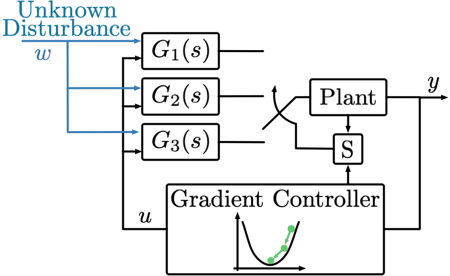
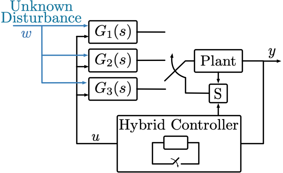
Figure 1: (left) A switched system in feedback with a gradient flow controller. (right) A switched system in feedback with a hybrid controller. “S” denotes a supervisory controller that actuates the switching between the modes of the plant.

3.1 Feedback Control via Online Gradient Descent

We first study the solution of the tracking Problem 2.1 via gradient descent flows of the form (3). The left scheme of Fig. 1 illustrates the approach. For such systems, the following two assumptions are standard.

Assumption 4.

The functions $\phi_{u}(\cdot)$ and $\phi_{y}(\cdot)$ are continuously differentiable, and their gradients are globally Lipschitz with constants $\ell_{u}>0$ and $\ell_{y}>0$, respectively.

Assumption 5.

For all $t\geq 0$, the function $\phi_{t}(u)$: (a) is radially unbounded, and (b) satisfies the Polyak-Łojasiewicz (PL) inequality, namely, $|{\nabla\phi_{t}(u)}|^{2}\geq 2\mu(\phi_{t}(u)-\phi_{t}(u_{t}^{*}))$, for some $\mu>0$ and for all $u\in{}^{m}$.

Under Assumption 4, the mapping $u\mapsto\phi_{t}(u)$ has a globally Lipschitz gradient with Lipschitz constant $\ell:=\ell_{u}+\ell_{y}|{G}|^{2}$. Similarly, Assumption 5 implies that $\phi_{t}(u)-\phi_{t}(u^{*})\geq\frac{\mu}{2}|{u-u_{t}^{*}}|^{2}$, $\forall~{}u\in\mathbb{R}^{m}$.

To design the controller we note that if $\omega_{t}$ and $H$ were known, the following dynamics can be shown to converge to $u_{t}^{*}$ under Assumptions 4 and 5 (see, for example, [24]):

$$\dot{u}=F_{GS}(u,\omega_{t}):=-\nabla\phi_{u}(u)-G^{\mathsf{T}}\nabla\phi_{y}(Gu+H\omega_{t}).$$ (9)

When $\omega_{t}$ and $H$ are unknown, we propose to approximate the steady-state output $Gu+H\omega_{t}$ with instantaneous feedback from the plant, leading to:

$${\dot{u}=F_{G}(u,y,\sigma):=-\eta_{\sigma}(\nabla\phi_{u}(u)+G^{\mathsf{T}}\nabla\phi_{y}(y)),}$$ (10)

where $\eta_{\sigma}>0$ is a mode-dependent tunable gain.

The system obtained by interconnecting plant (1), the switching signal generator (2.1), and the controller (10) leads to a HDS of the form (5), denoted by $\mathcal{H}_{G}$, with state $\varphi=(x,u,\chi,\omega_{t})$, continuous-time dynamics:

$$\dot{x} =P_{\sigma}(x,u,\omega_{t}), \dot{u} ={F_{G}(u,h(x,\omega_{t}),\sigma)},$$

$$\dot{\chi} \in F_{\chi}(\chi), \dot{\omega}_{t} =\Pi(\omega_{t})$$ (11)

flow set $C:={}^{n}\times{}^{m}\times C_{\chi}\times\Gamma$, discrete-time dynamics:

$$x^{+}=x,~{}~{}u^{+}=u,~{}~{}\chi^{+}\in G_{\chi}(\chi),~{}~{}\omega^{+}=\omega,$$ (12)

and jump set $D:={}^{n}\times{}^{m}\times D_{\chi}\times\Gamma$.

Next, we provide a result that establishes an explicit tracking bound for (3.1). To this end, we require that the controller gain satisfies $\eta_{\sigma}<\bar{\eta}_{\sigma}$, where

$$\bar{\eta}_{\sigma}=\frac{(1-\kappa)^{2}}{2-\kappa}\frac{\underline{\lambda}(Q_{\sigma})}{\ell_{y}|{C}||{G}||{P_{\sigma}A_{\sigma}^{\scalebox{0.75}[0.9]{$-$}1}B_{\sigma}}|},$$ (13)

where $(P_{\sigma},Q_{\sigma})$ are as in Assumption 1, and $\kappa\in(0,1)$. Moreover, we define the following constants:

$$\theta_{\sigma} :={\frac{1}{1+2|{P_{\sigma}A_{\sigma}^{\scalebox{0.75}[0.9]{$-$}1}B_{\sigma}}|}},$$ (14a)

$$\bar{a}_{\sigma} :=\frac{1}{\eta}\max\left\{(1\scalebox{0.75}[0.9]{$-$}\theta_{\sigma})\frac{\ell}{2},\theta_{\sigma}\bar{\lambda}(P_{\sigma})\right\},$$ (14b)

$$\underline{a}_{\sigma} :=\frac{1}{\eta}\min\left\{(1\scalebox{0.75}[0.9]{$-$}\theta_{\sigma})\frac{\mu}{2},\theta_{\sigma}\underline{\lambda}(P_{\sigma})\right\},$$ (14c)

$$b_{\sigma} =\frac{\kappa}{2}\min\left\{2\mu\eta_{\sigma},\frac{\underline{\lambda}(Q_{\sigma})}{\bar{\lambda}(P_{\sigma})}\right\},$$ (14d)

$$d_{\sigma} =\frac{2}{\kappa}\max\left\{\frac{\ell_{y}|{H}||{G}|}{\eta_{\sigma}\mu^{2}},\frac{2|{P_{\sigma}A_{\sigma}^{\scalebox{0.75}[0.9]{$-$}1}E_{\sigma}}|}{\underline{\lambda}(Q_{\sigma})}\right\},$$ (14e)

where $(\mu,\ell,\ell_{y},\ell_{u})$ are as in Assumptions 4 and 5.

Theorem 3.1.

Suppose that Assumptions 1-5 hold. If $\eta_{\sigma}\in(0,\bar{\eta}_{\sigma})$ for all $\sigma\in\mathcal{S}$ and the dwell-time satisfies $\tau_{d}>\frac{\ln a}{\min_{\sigma}b_{\sigma}}$, then the tracking error $\tilde{z}=z-z_{t}^{*}$ of the system $\mathcal{H}_{G}$ satisfies:

$$|\tilde{z}(t,j)|\leq a_{0}e^{-\frac{b_{0}t+c_{0}j}{2}}|\tilde{z}(t,j)|+a_{0}d_{0}\sup_{0\leq\tau\leq t}|{\dot{\omega}_{\tau}}|,$$ (15)

where $a_{0}=e^{\frac{\varrho}{2}N_{0}}\sqrt{a}$, $b_{0}=\min_{\sigma}b_{\sigma}-\frac{\varrho}{\tau_{d}}$, $c_{0}=\varrho-\ln a$, $d_{0}=\max_{\sigma}d_{\sigma}$, with $a:=\frac{\max_{\sigma}\bar{a}_{\sigma}}{\min_{\sigma}\underline{a}_{\sigma}}$ and $\varrho>0$ is any constant that satisfies $\ln a<\varrho<\tau_{d}\min_{\sigma}b_{\sigma}$. $\square$

This result establishes that a sufficiently-small gain $\eta_{\sigma}$ guarantees exponential convergence of $z$ to a neighborhood of the optimal trajectory $z_{t}^{*}$. As characterized by (13), the upper bound on the controller gain is proportional to the rate of convergence of the open-loop plant $\underline{\lambda}(Q_{\sigma})/\bar{\lambda}(P_{\sigma})$, and inversely proportional to the Lipschitz constant of the cost function $\ell_{y}$. Moreover, as characterized by (14d), the rate of decay of the tracking error is governed by the minimum between the rate of convergence of the controller (namely, $2\mu\eta_{\sigma}$) and the rate of convergence of the plant (namely, $\underline{\lambda}(Q_{\sigma})/\bar{\lambda}(P_{\sigma})$).

Remark 2.

The constants $(a_{0},b_{0},c_{0},d_{0})$ characterized in Theorem 3.1 depend on: (i)  $(\mu,\ell)$, which characterize the smoothness and gradient dominance of the steady state cost function (7); (ii) the matrices $(A_{\sigma},B_{\sigma},C_{\sigma},D_{\sigma},E_{\sigma})$ and $(Q_{\sigma},P_{\sigma})$, which govern the dynamics of the switched plant (1); and (iii) $(\tau_{d},N_{0})$ that govern the behavior of the signal $\sigma$ in (2.1). $\square$

Remark 3.

Assumption 5 is fundamental to guarantee exponential convergence. Indeed, as $\mu\rightarrow 0$, we have that $b_{\sigma}\rightarrow 0$ and $d_{\sigma}\rightarrow\infty$. Similar scenarios were recently investigated in [5, 4]. In contrast to these results, Theorem 3.1 accounts for time-varying disturbances, switching plant dynamics, and establishes an explicit exponential bound, as opposed to asymptotic convergence. $\square$

3.2 Feedback Control via Hybrid Gradient Descent

We now address Problem 2.1 by proposing a feedback controller inspired by the accelerated gradient method (4). To design the controller, we adapt (4) as follows: first we rewrite (4) as a set of first-order ODEs by letting $p=2$ and by defining the variables $u_{1}:=u$ and $u_{2}:=\frac{\tau}{2}\dot{u}_{1}+u_{1}$; second, we introduce an auxiliary state $u_{3}$ that models the evolution of a timer and replaces the temporal variable $\tau$, thus leading to the dynamics:

$$\dot{u}_{1} =\frac{2}{u_{3}}(u_{2}-u_{1})$$ (16a)

$$\dot{u}_{2} =-2ku_{3}\left(\nabla\phi_{u}(u_{1})+G^{\mathsf{T}}\nabla\phi_{y}(Gu_{1}+H\omega_{t})\right),$$ (16b)

$$\dot{u}_{3} =\frac{1}{2}.$$ (16c)

The choice of the variables $(u_{1},u_{2},u_{3})$ is inspired by accelerated momentum-based optimization and estimation algorithms proposed in e.g. [13, Eq. (14)], [16], and [15]. Further, we note that the choice $\dot{u}_{3}=1/2$, also used in [15] to solve static optimization problems, is motivated by our Lyapunov-based analysis, presented below.

Remark 4.

As shown in [19, Prop. 1] and [20, Thm. 1], the convergence of (16) lacks uniformity with respect to the initial value of $u_{3}$. In turn, this precludes the application of standard multi-time scale techniques using quadratic-type Lyapunov functions [10, pp. 453] or regular perturbations techniques, see [21, Thm. 1]. $\square$

Similarly to (9), the dynamics (16) require knowledge of $H$ and $\omega_{t}$ to be implemented. Hence, we propose to approximate the steady-state map $Gu_{1}+H\omega_{t}$ with the instantaneous output $y$ of the dynamical system. While this modification leads to an accelerated version of the controller proposed in Section 3.1, empirical and theoretical evidence suggests that such modifications are not sufficient to guarantee tracking of the optimal trajectories (see Remark 4). To address this limitation, we introduce discrete-time resets of the state variables of (16), which resemble the “restarting” heuristics used in the literature of machine learning [14, 13, 25] and hybrid control [26]. The proposed controller is then hybrid, with state $u=(u_{1},u_{2},u_{3})$, continuous-time dynamics

$$\dot{u}=F_{H}(u,y,\sigma):=\eta_{\sigma}\left(\begin{array}[]{c}\dfrac{2}{u_{3}}(u_{2}-u_{1})\\ -2ku_{3}\left(\nabla\phi_{u}(u_{1})+G^{\mathsf{T}}\nabla\phi_{y}(y)\right)\\ \frac{1}{2}\end{array}\right),$$

where $\eta_{\sigma}>0$ is a mode-dependent tunable gain; flow set $C_{H}=\mathbb{R}^{n}\times\mathbb{R}^{n}\times[\delta,\Delta]$, where $\Delta>\delta>0$ are tunable parameters characterizing the restarts of the timer variable; discrete-time dynamics

$$u^{+}=G_{H}(u):=R_{0}u,~{}~{}R_{0}=\left[\begin{array}[]{ccc}I&0&0\\ r_{0}I&(1-r_{0})I&0\\ 0&0&\frac{\delta}{\Delta}\end{array}\right],$$

where $r_{0}\in\{0,1\}$ is the reset policy of the controller; and jump set $D_{H}=\mathbb{R}^{n}\times\mathbb{R}^{n}\times\{\Delta\}$.

In words, the logic of the controller is as follows: when the timer $u_{3}$ is equal to $\Delta$, the controller states $(u_{1},u_{2})$ are re-initialized and the timer variable is reset to the value $\delta$. Notice that when $r_{0}=0$, only the timer $u_{3}$ is reset to $\delta$, whereas when $r_{0}=1$ both the momentum variable $u_{2}$ is re-initialized to $u_{1}$ and the timer $u_{3}$ is reset to $\delta$. By recalling the definition of $u_{2}$, we notice that the latter restarting policy corresponds to setting the momentum $\dot{u}_{1}$ to zero.

The interconnection of the hybrid controller and the switched LTI plant (1) leads to a HDS with state $\varphi=(x,u,\chi,\omega_{t})$, continuous-time dynamics:

$$\dot{x} =P_{\sigma}(x,u,\omega_{t}), \dot{u} ={F_{H}(u,h(x,\omega_{t}),\sigma)},$$

$$\dot{\chi} \in F_{\chi}(\chi), \dot{\omega}_{t} =\Pi(\omega_{t})$$ (17)

and flow set $C=\mathbb{R}^{n}\times C_{H}\times C_{\chi}\times\Gamma$. Jumps in the closed-loop system can be triggered by both switches of the plant and by resets of the controller. Therefore, the discrete-time dynamics are captured by the inclusion:

$$\varphi\in D:=D_{1}\cup D_{2},~{}~{}~{}\varphi^{+}\in G(\varphi),$$ (18)

where the set-valued map $G$ and the sets $D_{1},D_{2}$ are

$$G(\varphi):=\left\{\begin{array}[]{l}G_{1}(\varphi),~{}~{}~{}~{}\varphi\in D_{1}:=\mathbb{R}^{n}\times C_{H}\times D_{\chi}\times\Gamma\\ G_{2}(\varphi),~{}~{}~{}~{}\varphi\in D_{2}:=\mathbb{R}^{n}\times D_{H}\times C_{\chi}\times\Gamma\\ G_{1}(\varphi)\cup G_{2}(\varphi),~{}~{}~{}\varphi\in D_{1}\cap D_{2},\end{array}\right.$$ (19)

with $G_{1}(\varphi):=\{x\}\times\{u\}\times G_{\chi}(\chi)\times\{\omega_{t}\}$ and $G_{2}(\varphi):=\{x\}\times\{G_{H}(u)\}\times\{\chi\}\times\{\omega_{t}\}$. We denote the hybrid system (3.2)-(19) in compact form by $\mathcal{H}_{H}$.

Remark 5.

Notice that the model (3.2)-(19) naturally captures non-uniqueness of solutions that can emerge when the plant and the controller are in their jump sets simultaneously. In these scenarios, arbitrarily-small disturbances may force the plant or the controller to jump before the other, and a well-posed model of the hybrid dynamics allows us to capture both behaviors of the system as the disturbance vanishes. $\square$

Next, we provide error-tracking guarantees for $\mathcal{H}_{H}$. To this end, we first consider the case where the disturbance $\omega_{t}$ is constant, and we show that the (time-invariant) optimizer is globally practically asymptotically stable.

Remark 6.

Since we first focus on asymptotic stability properties, it suffices to consider plants (1) with a single mode (i.e., $\mathcal{S}:=\{\sigma\}$). Indeed, if each individual mode in $\mathcal{S}$ leads to asymptotic stability of the closed-loop system, then semi-global practical asymptotic stability (with respect to $\tau_{d}^{-1}$ in (2.1)) for the system with multiple modes will follow directly from [11, Corollary 7.28]. $\square$

We begin by introducing an inverse Lipschitz-type assumption.

Assumption 6.

The function $u\mapsto\phi_{t}(u)$ is convex, radially unbounded, and for each $\nu_{0}>0$ there exists $\ell_{0}>0$ such that $|{u-u_{t}^{*}}|\geq\nu_{0}$ for some $u\in{}^{m}$ implies $|{\nabla\phi_{t}(u)}|\geq\ell_{0}|{u-u_{t}^{*}}|$. $\square$

Next, we require that the controller gain satisfies $\eta_{\sigma}<\bar{\eta}_{\sigma}$, where

$$\bar{\eta}_{H}=\frac{\underline{\lambda}(Q_{\sigma})}{2\ell_{y}|{C}||{G}|}\min\left\{\frac{1}{2k\delta\Delta|{P_{\sigma}A_{\sigma}^{\scalebox{0.75}[0.9]{$-$}1}B_{\sigma}}|},\frac{\theta\ell_{0}^{2}\delta\kappa^{2}k}{2(1-\theta)\ell\Delta|{C}||{G}|}\right\}.$$

with $\kappa\in(0,1)$ and

$$\theta=\frac{\ell_{y}k\Delta|{C}||{G}|}{\ell_{y}k\Delta|{C}||{G}|+2\delta|{P_{\sigma}A_{\sigma}^{\scalebox{0.75}[0.9]{$-$}1}B_{\sigma}}|}.$$

Using this gain we obtain the following result:

Theorem 3.2.

Let Assumptions 1-4 and 6 hold, and assume that $\omega_{t}:=\omega\in\mathbb{R}^{q}$ is constant, that the plant has a single mode $\mathcal{S}=\{\sigma\}$, and let the reset policy be $r_{0}=0$. If $\eta_{\sigma}\in(0,\bar{\eta}_{\sigma})$, then any solution of $\mathcal{H}_{H}$ satisfies:

$$a)~{}\limsup_{t+j\rightarrow\infty}|z(t,j)-z^{*}|\leq\nu_{0},~{}~{}~{}~{}~{}~{}~{}~{}~{}\forall(t,j)\in\text{dom}(\varphi).$$

$$b)~{}\phi(u_{1}(t,j))-\phi(u^{*})\leq\frac{\alpha_{j}}{u_{3}^{2}(t,j)}+\nu_{0},~{}\forall(t,j)\in\text{dom}(\varphi),t>\underline{t}_{j},$$

where $\alpha_{j}>0$, $z:=(x,u_{1})$, $z^{*}:=(x^{*},u^{*})$, and $\underline{t}_{j}:=\min\{t\geq 0:(t,j)\in\text{dom}(\varphi)\}$. $\square$

The convergence result of Theorem 3.2 is global, but of “practical” nature. Namely, convergence is achieved only to a $\nu_{0}$-neighborhood of the optimal set via the choice of $\bar{\eta}_{\sigma}$, which, in turn, depends on the constant $\ell_{0}$. Two main comments are in order. First, the upper bound on the controller gain $\bar{\eta}_{\sigma}$ shrinks to zero when either $\delta\to 0^{+}$ or $\Delta\to\infty$. Since $\delta=0$ and $\Delta=\infty$ correspond to the (non-restarted ODE) (4), our analysis suggests that for (4) there may exist no gain $\eta>0$ that guarantees stability for the closed-loop system: a similar observation was recently made in [4, Sec. IV.B]. Second, the result establishes that the error in the steady-state cost function decreases (outside a neighborhood of the optimal point) at a rate of order $\mathcal{O}(c_{j}/u_{3}^{2})$ during the $j^{th}$ interval of flow, where $c_{j}$ is constant in each interval. Thus, the larger the difference $\Delta-\delta$, the larger the size of the intervals where this bound holds. This can be seen as a semi-acceleration property that holds during flows. Indeed, using the definition of $u_{3}$, during the first interval of flow we have that $u_{3}(t,0)=u_{3}(0,0)+0.5t$, and the error in the cost decreases at a rate $\mathcal{O}(c_{0}/t^{2})$; see also [14, 13, 15] for similar bounds in static optimization problems. We also note that, as revealed by the proof (presented below), and in contrast to the case of optimization problems without plants in the loop, the quantity $\alpha_{j}$ in item b) explicitly depends on the LTI plant (1) via the matrix $P_{\sigma}$. Finally, we note that as $\nu_{0}\rightarrow 0$, the controller gain might satisfy $\eta\rightarrow 0$, as shown in the following example.

Example 7.

Let $\phi(u_{1})=\frac{1}{\theta}(|{u_{1}-u^{*}}|^{\theta}+|{Gu_{1}+H\omega_{t}}|^{\theta})$, with $\theta\in\mathbb{Z}_{\geq 2}$, which is not strongly convex when $\theta>2$. Also, let $G=[g_{ij}]$ with $g_{ij}\geq 0$ for all $i,j$, as it is the case in compartmental systems [9]. It then follows that $|{\nabla\phi(u_{1})}|\geq|{u_{1}-u_{t}^{*}}|^{\theta-1}\geq\nu_{0}^{\theta-2}|{u_{1}-u_{t}^{*}}|$. Thus, $\phi_{t}$ satisfies Assumption 6 with $\ell_{0}=\nu_{0}^{\theta-2}$. Note that in this case, as $\nu_{0}\to 0^{+}$, the admissible constant $\ell_{0}$ and the controller gain $\bar{\eta}_{\sigma}$ shrink to zero. This relation suggests that as the size of the neighborhood satisfies $\nu_{0}\rightarrow 0$, the controller gain also satisfies $\eta\rightarrow 0$. $\square$

Next, under the following strong convexity assumption, we will show that the hybrid controller can solve Problem 1 with an exponential rate of convergence.

Assumption 7.

There exists $\mu\in{}_{>0}$ such that $\phi_{t}(u)\geq\phi_{t}(u^{\prime})+\nabla\phi_{t}(u^{\prime})^{\mathsf{T}}(u-u^{\prime})+\frac{\mu}{2}|{u-u^{\prime}}|^{2}$ holds for all $u,u^{\prime}\in{}^{m}$, and all $t\geq 0$.

To establish an exponential tracking bound, we require that the controller gain satisfies $\eta_{\sigma}<\bar{\eta}_{\sigma}$, where

$$\bar{\eta}_{\sigma} ={\frac{(1-\kappa)^{2}}{16}\frac{\delta\underline{\lambda}(Q_{\sigma})}{k\Delta\ell_{y}|{C}||{G}||{P_{\sigma}A_{\sigma}^{\scalebox{0.75}[0.9]{$-$}1}B_{\sigma}}|},} \kappa \in(0,1).$$ (20)

Moreover, we define the following constants:

$$\theta_{\sigma} ={\frac{k\Delta\ell_{y}|{C}||{G}|}{k\Delta\ell_{y}|{C}||{G}|+2\delta^{\scalebox{0.75}[0.9]{$-$}1}|{P_{\sigma}A_{\sigma}^{\scalebox{0.75}[0.9]{$-$}1}B_{\sigma}}|}},$$ (21a)

$$\bar{a}_{\sigma} :={\max\left\{(1-\theta_{\sigma})\frac{1+k\ell\Delta^{2}}{2},\theta_{\sigma}\bar{\lambda}(P_{\sigma})\right\}},$$ (21b)

$$\underline{a}_{\sigma} :={\min\left\{(1-\theta_{\sigma})\frac{1+2k\ell\Delta^{2}}{4},\theta_{\sigma}\underline{\lambda}(P_{\sigma})\right\}},$$ (21c)

$$b_{\sigma} ={\frac{\kappa}{2}\min\left\{\frac{2\eta_{\sigma}}{\Delta(1+2k\ell\Delta^{2})},\frac{\eta_{\sigma}k\delta\mu}{2(1+2k\ell\Delta^{2})},\frac{\underline{\lambda}(Q_{\sigma})}{\bar{\lambda}(P_{\sigma})}\right\}},$$ (21d)

$$d_{\sigma} ={\frac{2}{\kappa}\max\left\{\frac{\bar{d}_{\sigma}}{\eta_{\sigma}\min\{\Delta^{\scalebox{0.75}[0.9]{$-$}1},k\delta\mu/4\}},\frac{2|{P_{\sigma}A_{\sigma}^{\scalebox{0.75}[0.9]{$-$}1}E_{\sigma}}|}{\underline{\lambda}(Q_{\sigma})}\right\}}.$$ (21e)

where $\bar{d}_{\sigma}:=\sqrt{2}k\Delta^{2}\ell_{y}|{H}||{G}|+\sqrt{2}\max_{\omega\in\Gamma}|{\frac{\partial u^{*}}{\partial\omega}}|(k\Delta^{2}+\frac{1}{2}(1+2k\Delta^{2}\ell))$.

Theorem 3.3.

Let Assumptions 1-4 and 7 hold and let the reset policy be $r_{0}=1$. If $\eta_{\sigma}\in(0,\bar{\eta}_{\sigma})$ for all $\sigma\in\mathcal{S}$, the timer thresholds satisfy $\Delta^{2}-\delta^{2}>\frac{1}{2k\mu}$, and the dwell-time satisfies $\tau_{d}>\frac{\ln a}{\min_{\sigma}b_{\sigma}}$, then the tracking error $\tilde{z}=z-z_{t}^{*}$ of the system $\mathcal{H}_{H}$ satisfies:

$$|\tilde{z}(t,j)|\leq a_{0}e^{-\frac{b_{0}t+c_{0}j}{2}}|\tilde{z}(t,j)|+a_{0}d_{0}\sup_{0\leq\tau\leq t}|{\dot{\omega}_{\tau}}|,$$ (22)

where $a_{0}=e^{\frac{\varrho}{2}N_{0}}\sqrt{a}$, $b_{0}=\min_{\sigma}b_{\sigma}-\frac{\varrho}{\tau_{d}}$, $c_{0}=\varrho-\ln a$, $d_{0}=\max_{\sigma}d_{\sigma}$, with $a:=\frac{\max_{\sigma}\bar{a}_{\sigma}}{\min_{\sigma}\underline{a}_{\sigma}}$ and $\varrho>0$ is any constant that satisfies $\ln a<\varrho<\tau_{d}\min_{\sigma}b_{\sigma}$. $\square$

The result of Theorem 3.3 requires three types of conditions on the controller parameters: (i) a sufficiently-small choice of the controller gain $\eta_{\sigma}$, (ii) a quadratic-like dwell-time condition $\Delta^{2}-\delta^{2}>1/2k\mu$, which gives a lower bound on the restarting frequency, and (iii) an average dwell-time condition imposed on the switching signal $\sigma$.

Remark 8.

The result of Theorem 3.3 leverages the resets of the momentum $\dot{u}$. Similar “restarting” techniques have been studied in literature of optimization and machine learning [14, 13], with optimal restarting frequencies presented in [25, Thm. 3.1], [15, Sec. 3.2.1]. For example, in [15, Sec. 3.2.1], it is shown that, as $\delta\to 0^{+}$, the choice $\Delta=e\sqrt{\frac{1}{2k\mu}+\delta^{2}}$ with $k=1/2\ell$ can achieve exponential convergence of order $\mathcal{O}(e^{-t\sqrt{\mu/\ell}})$. This is particularly advantageous in problems with condition numbers satisfying $\ell/\mu\gg 1$. In the context of feedback-based optimization, the advantages of using momentum are recovered as the time scale separation between the plant and the controller increases. Numerical experiments are presented in Section 5. $\square$

We conclude by noting that the closed-loop systems $\mathcal{H}_{H}$ with constant disturbances $\omega_{t}=\omega$ are robust to small bounded additive disturbances $t\mapsto e(t)$ acting on the states and dynamics of the system. Indeed, by construction, the hybrid system $\mathcal{H}_{H}$ is well-posed and it satisfies the Basic Conditions [11, Assump. 6.5]. Therefore, the robustness property follows directly by [11, Cor. 7.27].

4 Proofs

To prove our main results, we use tools from HDS theory [11]. We model the closed-loop system as a time-invariant and well-posed HDS described by the interconnection between the exosystem (8), the plant (1), the switching generator (2.1), and the controller. For this interconnection, we construct a hybrid Lyapunov function to guarantee stability of the closed-loop dynamics. The construction of the Lyapunov functions is inspired by singular perturbation arguments [10], adjusted to account for the switching dynamics and the hybrid controllers. This construction allows us to derive conditions on $\eta_{\sigma}$ and on the dwell-time parameters of $\sigma$ to guarantee suitable asymptotic or exponential input-to-state stability with respect to $\dot{\omega}$. Since the closed-loop system can be modeled as a time-invariant HDS, in our analysis we drop the subscript $t$ from the signal $\omega$, the optimizer $u^{*}(\omega)$, and the cost function (7), which we write as an explicit function of $u$ and $\omega$ of the form $\phi(u,\omega)$.

4.1 Proof of Theorem 3.1

We divide the proof into four main steps.

Step 1. Consider the change of variable $\tilde{u}:=u-u^{*}(\omega)$, and $\tilde{x}:=x-\left(-A_{\sigma}^{\scalebox{0.75}[0.9]{$-$}1}B_{\sigma}(\tilde{u}+u^{*}(\omega))-A_{\sigma}^{\scalebox{0.75}[0.9]{$-$}1}E_{\sigma}\omega\right)$, which denote the tracking error of the plant and the controller, respectively. The dynamics of $\tilde{u}$ are:

$$\dot{\tilde{u}} =\dot{u}-\dot{\overbrace{u^{*}(\omega)}}=-\eta\Big{(}\nabla\phi_{u}(\tilde{u}+u^{*}(\omega))$$

$$\quad+G^{\mathsf{T}}\nabla\phi_{y}\big{(}C\tilde{x}+G(\tilde{u}+u^{*}(\omega))+H\omega\big{)}\Big{)}-\dot{\overbrace{u^{*}(\omega)}}$$

$$=:\eta\psi_{c}(\tilde{x},\tilde{u},\omega)-\dot{\overbrace{u^{*}(\omega)}},$$ (23)

and note that $\psi_{c}(0,\tilde{u},\omega)=-\nabla_{u}\phi(\tilde{u}+u^{*}(\omega),\omega)$. Also

$$\dot{\tilde{x}} =A_{\sigma}\tilde{x}+\eta A_{\sigma}^{-1}B_{\sigma}\psi_{c}(\tilde{x},\tilde{u},\omega)+A_{\sigma}^{-1}E_{\sigma}\dot{\omega}.$$ (24)

Next, we consider the Lyapunov-like function

$$V_{\sigma}(\tilde{z},\omega)=\frac{(1-{\theta_{\sigma}})}{\eta}V_{1}(\tilde{u},\omega)+\frac{{\theta_{\sigma}}}{\eta}V_{2}(\tilde{x},\sigma),$$ (25)

with $\tilde{z}=(\tilde{x},\tilde{u})$ and $\theta_{\sigma}\in(0,1)$ is as in (14), and $V_{1}(\tilde{u},\omega):=\phi(\tilde{u}+u^{*}(\omega),\omega)-\phi(u^{*}(\omega),\omega)$, $V_{2}(\tilde{x},\sigma):=\tilde{x}^{\mathsf{T}}P_{\sigma}\tilde{x},$ with $P_{\sigma}$ given by Assumption 1. The function ${V_{\sigma}}$ is a convex combination of a Lyapunov-like function for the plant and a Lyapunov-like function for a standard gradient flow. By Assumption 1, we have that $\underline{\lambda}(P_{\sigma})|\tilde{x}|^{2}\leq V_{2}(\tilde{x})\leq\overline{\lambda}(P_{\sigma})|\tilde{x}|^{2}$. Also, by Assumptions 4 and 5, we have that $\frac{\mu}{2}|\tilde{u}|^{2}\leq V_{1}(\tilde{u},\omega)\leq\frac{\ell}{2}|\tilde{u}|^{2}$, for all $\omega\in\Gamma$. Therefore, $\underline{a}|\tilde{z}_{\sigma}|^{2}\leq V_{\sigma}(\tilde{z},\omega)\leq\bar{a}_{\sigma}|z|^{2}$, for all $\omega\in\Gamma$, with $\bar{a}_{\sigma}$ and $\underline{a}_{\sigma}$ given by (14b) and (14c).

Step 2. Next, we show that for each fixed mode $\sigma\in\mathcal{S}$, and outside a neighborhood of the origin that is proportional in size to ${|\dot{\omega}|}$, the function ${V_{\sigma}}$ decreases along the trajectories of (23) and (24) at an exponential rate. In particular, note that

$$\frac{1}{\eta}\nabla_{\tilde{u}}V_{1}^{\top}\dot{\tilde{u}} =-\psi_{c}(0,\tilde{u},\omega)^{\top}\Big{(}\psi_{c}(\tilde{x},\tilde{u},\omega)-\frac{1}{\eta}\dot{\overbrace{u^{*}(\omega)}}\Big{)}$$

$$\leq-|{\psi_{c}(0,\tilde{u},\omega)}|^{2}+a_{2}|{\psi_{c}(0,\tilde{u},\omega)}||{\tilde{x}}|$$

$$~{}~{}~{}+\frac{1}{\eta}\psi_{c}(0,\tilde{u},\omega)^{\top}\frac{\partial u^{*}}{\partial\omega}\dot{\omega},$$

where the last inequality follows by Assumption 4 with $a_{2}:=\ell_{y}|{C}||{G}|$. Similarly, we have that

$$\nabla_{\omega}V_{1}^{\top}\dot{\omega}=\left(\nabla_{\omega}\phi(\tilde{u}+u^{*}(\omega),\omega)-\nabla_{\omega}\phi(u^{*}(\omega),\omega)\right)^{\top}\dot{\omega}.$$ (26)

Using the structure of $\phi$, and the chain rule:

$$\nabla_{\omega}\phi =\frac{\partial u^{*}}{\partial\omega}^{\top}\nabla\phi_{u}+H^{\top}\nabla\phi_{y}+\frac{\partial u^{*}}{\partial\omega}^{\top}G^{\top}\nabla\phi_{y}$$

$$=\frac{\partial u^{*}}{\partial\omega}^{\top}\nabla_{u}\phi+H^{\top}\nabla\phi_{y}.$$ (27)

Since $\nabla_{u}\phi(u^{*}(\omega))=0$, and using the definition of $\psi_{c}(0,\tilde{u},\omega)$, it follows that

$$\nabla_{\omega}V_{1}^{\top}\dot{\omega} \leq-\left(\frac{\partial u^{*}}{\partial\omega}^{\top}\psi_{c}(0,\tilde{u},\omega)\right)^{\top}\dot{\omega}+\ell_{y}|H||G||\tilde{u}||\dot{\omega}|.$$

where we used again Assumption 4. Since $\dot{V}_{1}=\nabla_{\tilde{u}}V_{1}^{\top}\dot{\tilde{u}}+\nabla_{\omega}V_{1}^{\top}\dot{\omega}$, we have

$$\frac{1}{\eta}\dot{V}_{1} \leq-|{\psi_{c}(0,\tilde{u},\omega)}|^{2}+a_{2}|{\psi_{c}(0,\tilde{u},\omega)}||{\tilde{x}}|$$

$$~{}~{}~{}~{}+\frac{1}{\eta}\psi_{c}(0,\tilde{u},\omega)^{\top}\frac{\partial u^{*}}{\partial\omega}\dot{\omega}-\frac{1}{\eta}\left(\frac{\partial u^{*}}{\partial\omega}^{\top}\psi_{c}(0,\tilde{u},\omega)\right)^{\top}\dot{\omega}$$

$$~{}~{}~{}~{}+\frac{\ell_{y}}{\eta}|H||G|\frac{|\psi_{c}(0,\tilde{u},\omega)|}{\mu}|\dot{\omega}|,$$

$$\leq-|{\psi_{c}(0,\tilde{u},\omega)}|^{2}+a_{2}|{\psi_{c}(0,\tilde{u},\omega)}||{\tilde{x}}|$$

$$~{}~{}~{}~{}+\frac{\ell_{y}}{\eta\mu}|H||G||\psi_{c}(0,\tilde{u},\omega)||\dot{\omega}|,$$

where the last term follows from the quadratic growth inequality. Using $|{\nabla_{u}\phi}|^{2}\geq 2\mu V_{1}$, we obtain:

$$\frac{1}{\eta}\dot{V}_{1}\leq-a_{1}|{\psi_{c}(0,\tilde{u},\omega)}|^{2}+a_{2}|{\psi_{c}(0,\tilde{u},\omega)}||{\tilde{x}}|-a_{3}V_{1}(\tilde{u},\omega),$$

where $a_{1}=(1-\kappa)$ and $a_{3}=\kappa\mu$, which holds whenever $|{\psi_{c}(0,\tilde{u},\omega)}|\geq\frac{2\ell_{y}|{H}||{G}|}{\kappa\eta\mu}{|{\dot{\omega}}|}$. Since $|{\psi_{c}(0,\tilde{u},\omega)}|\geq\mu|{\tilde{u}}|$, a sufficient condition for the above inequality to hold is $|{\tilde{u}}|\geq\frac{2\ell_{y}|{H}||{G}|}{\kappa\eta\mu^{2}}{|{\dot{\omega}}|}$.

On the other hand, for each fixed $\sigma\in\mathcal{S}$, we have:

$$\frac{1}{\eta}\dot{V}_{2} =2\tilde{x}^{\mathsf{T}}P_{\sigma}\left(\frac{1}{\eta}A_{\sigma}\tilde{x}+A_{\sigma}^{\scalebox{0.75}[0.9]{$-$}1}B_{\sigma}\psi_{c}(\tilde{x},\tilde{u},\omega)+\frac{1}{\eta}A_{\sigma}^{\scalebox{0.75}[0.9]{$-$}1}E_{\sigma}\dot{\omega}\right)$$

$$\leq-\frac{\underline{\lambda}(Q_{\sigma})}{\eta}|{\tilde{x}}|^{2}+2|{P_{\sigma}A_{\sigma}^{\scalebox{0.75}[0.9]{$-$}1}B_{\sigma}}||{\tilde{x}}||{\psi_{c}(\tilde{x},\tilde{u},\omega)}|$$

$$\quad\quad+\frac{2}{\eta}|{P_{\sigma}A_{\sigma}^{\scalebox{0.75}[0.9]{$-$}1}E_{\sigma}}||{\tilde{x}}||{\dot{\omega}}|,$$ (28)

where the inequality follows from Assumption 1. Since $|\psi_{c}(\tilde{x},\tilde{u},\omega)|\leq|{\psi_{c}(0,\tilde{u},\omega)}|+a_{2}|{\tilde{x}}|$, and $V_{2}(\tilde{x},\sigma)\leq\bar{\lambda}(P_{\sigma})|{\tilde{x}}|^{2}$, we can further upper bound (28) as:

$$\frac{1}{\eta}\dot{V}_{2}\leq-\frac{b_{1}}{\eta}|{\tilde{x}}|^{2}+b_{2}|{\tilde{x}}||{\psi_{c}(0,\tilde{u},\omega)}|+b_{3}|{\tilde{x}}|^{2}-b_{4}V_{2}(\tilde{x},\sigma)$$

which holds whenever $|{\tilde{x}}|\geq\frac{4|{P_{\sigma}A_{\sigma}^{\scalebox{0.75}[0.9]{$-$}1}E_{\sigma}}|}{\kappa\underline{\lambda}(Q_{\sigma})}{|{\dot{\omega}}|}$, where $b_{1}:=(1-\kappa)\underline{\lambda}(Q_{\sigma})$, $b_{2}:=2|{P_{\sigma}A_{\sigma}^{\scalebox{0.75}[0.9]{$-$}1}B_{\sigma}}|$, $b_{3}:=2a_{2}|{P_{\sigma}A_{\sigma}^{\scalebox{0.75}[0.9]{$-$}1}B_{\sigma}}|$, and $b_{4}:=\frac{\kappa}{2\eta}\frac{\underline{\lambda}(Q_{\sigma})}{\bar{\lambda}(P_{\sigma})}$.

Step 3. Next, using the bounds on $\dot{V}_{1}$ and $\dot{V}_{2}$, we obtain that for each fixed $\sigma\in\mathcal{S}$ the function $V_{\sigma}$ satisfies the following bound outside a $|\dot{\omega}|$-neighborhood of the origin:

$$\dot{V}_{\sigma} \leq-\xi^{\mathsf{T}}\Lambda_{\sigma}\xi-{\frac{\kappa}{2}\min\left\{2\eta\mu,\frac{\underline{\lambda}(Q_{\sigma})}{\bar{\lambda}(P_{\sigma})}\right\}}V_{\sigma}(\tilde{z},\omega),$$ (29)

where $\xi=(|{\nabla\phi(\tilde{u}+u^{*}(\omega),\omega)}|,|{\tilde{x}}|)$ and $\Lambda_{\sigma}$ is a $2\times 2$ symmetric matrix with entries $\Lambda_{11}=(1-\theta)a_{1}$, $\Lambda_{12}=\Lambda_{12}=-\frac{1}{2}((1-\theta)a_{2}+\theta b_{2})$, and $\Lambda_{22}=\theta(b_{1}/\eta-b_{3})$. Since the largest $\theta\in(0,1)$ that guarantees $\Lambda\succ 0$ is as in (14), we conclude that $\Lambda\succ 0$ when $\eta_{\sigma}\in(0,\bar{\eta}_{\sigma})$, with $\bar{\eta}_{\sigma}$ as in (13).

Step 4. Finally, we incorporate the switches of the plant which are governed by the states $(\sigma,\tau)$ generated by (2.1). Using $V_{\sigma}$, we consider the extended function $W(\tilde{\vartheta})=e^{\varrho\tau}V_{\sigma}(\tilde{z},\omega)$, where $\varrho>0$ and $\tilde{\vartheta}:=(\tilde{z},\sigma,\tau,\omega)$. We will show the existence of $\varrho$ such that $W$ is a hybrid ISS Lyapunov function for the HDS with dynamics (2.1), (8), and (23)-(24), with respect to the “input” $|\dot{\omega}|$, and the compact set $\mathcal{A}_{1}:=\left\{\tilde{\vartheta}:\tilde{z}=0,~{}\sigma\in\mathcal{S},~{}\tau\in[0,N_{0}],~{}\omega\in\Gamma\right\}$. Indeed, note that for all $\tilde{z}\in\mathbb{R}^{n+m}$, all $(\tau,\sigma)\in[0,N_{0}]\times\mathcal{S}$, and $\omega\in\Gamma$, we have that $\min_{\sigma}\underline{a}_{\sigma}|{\tilde{z}}|^{2}\leq W(\tilde{\vartheta})\leq e^{\varrho N_{0}}\max_{\sigma}\bar{a}_{\sigma}|{\tilde{z}}|^{2}$, where $\underline{a}_{\sigma},\bar{a}_{\sigma}$ are as in (14). During flows, we have that:

$$\dot{W}=e^{\varrho\tau}(\varrho V_{\sigma}\dot{\tau}+\dot{V}_{\sigma})\leq\left(\frac{\varrho}{\tau_{d}}-\min_{\sigma}b_{\sigma}\right)W(\tilde{\vartheta}),$$

where $b_{\sigma}$ is as in (14d), which holds whenever $|{\tilde{u}}|\geq{\frac{2\ell_{y}|{H}||{G}|}{\kappa\eta\mu^{2}}|{\dot{\omega}}|}$ and $|{\tilde{x}}|\geq{\frac{4|{P_{\sigma}A_{\sigma}^{\scalebox{0.75}[0.9]{$-$}1}E_{\sigma}}|}{\kappa\underline{\lambda}(Q_{\sigma})}|{\dot{\omega}}|}$. Hence, $W$ decreases during flows if $\varrho<\tau_{d}\min_{\sigma}b_{\sigma}$. Next, note that at each jump we have that $\tilde{x}^{+}=\tilde{x}$, $\tilde{u}^{+}=\tilde{u}$, $\sigma^{+}\in\mathcal{S}$, $\omega^{+}=\omega$, and $\tau^{+}=\tau-1$. Hence, $W(\tilde{\vartheta}^{+})\leq e^{\varrho\tau^{+}}\max_{\sigma}V_{\sigma}(\tilde{z}^{+},\omega^{+})$ and $W(\tilde{\vartheta}^{+})\leq e^{-\varrho+\ln(\max_{\sigma}\bar{a}_{\sigma})-\ln(\min_{\sigma}\underline{a}_{\sigma})}W(\tilde{\vartheta})$. It follows that if $\varrho>\ln\left(\max_{\sigma}\bar{a}_{\sigma}/\min_{\sigma}\underline{a}_{\sigma}\right)$, the function $W$ also decreases during jumps. It follows that if $\tau_{d}>\frac{\ln(\max_{\sigma}\bar{a}_{\sigma}/\min_{\sigma}\underline{a}_{\sigma})}{\min_{\sigma}b_{\sigma}}$, then $W$ is a hybrid ISS Lyapunov function for the closed-loop system with “input” $\dot{\omega}$. The quadratic bounds and the periodic nature of the jumps imply exponential input-to-state stability of $\mathcal{A}_{1}$, with input $|\dot{\omega}|$. $\blacksquare$

4.2 Proof of Theorem 3.3

We follow similar steps to the proof of Theorem 3.1, now incorporating the jumps of the hybrid controller.

Step 1. Let $\tilde{u}_{1}:=u_{1}-u^{*}(\omega)$, $\tilde{u}_{2}:=u_{2}-u^{*}(\omega)$, $\tilde{u}_{3}=u_{3}$, and $\tilde{x}:=x+A_{\sigma}^{\scalebox{0.75}[0.9]{$-$}1}B_{\sigma}(\tilde{u}_{1}+u^{*}(\omega))+A_{\sigma}^{\scalebox{0.75}[0.9]{$-$}1}E_{\sigma}\omega$. The error dynamics of $\tilde{u}=(\tilde{u}_{1},\tilde{u}_{2},\tilde{u}_{3})$ are given by $\dot{\tilde{u}}_{3}=\frac{\eta}{2}$, and

$$\dot{\tilde{u}}_{1} =\dfrac{2\eta}{\tilde{u}_{3}}(\tilde{u}_{2}-\tilde{u}_{1})-\dot{\overbrace{u^{*}(\omega)}},$$

$$\dot{\tilde{u}}_{2} =2k\eta\tilde{u}_{3}\psi_{c}(\tilde{x},\tilde{u}_{1},\omega)-\dot{\overbrace{u^{*}(\omega)}},$$ (30)

where $\psi_{c}$ was defined in (23). Also, we have

$$\dot{\tilde{x}}=A_{\sigma}\tilde{x}+\frac{2\eta}{\tilde{u}_{3}}A_{\sigma}^{-1}B_{\sigma}(\tilde{u}_{2}-\tilde{u}_{1})+A_{\sigma}^{-1}E_{\sigma}\dot{\omega}.$$ (31)

We consider the Lyapunov-like function:

$$V_{\sigma}(\tilde{z},\omega)=\frac{(1-{\theta_{\sigma}})}{{\eta_{\sigma}}}V_{1}(\tilde{u},\omega)+\frac{{\theta_{\sigma}}}{{\eta_{\sigma}}}V_{2}(\tilde{x},\sigma),~{}$$ (32)

where $\theta_{\sigma}\in(0,1)$, $\tilde{z}:=(\tilde{x},\tilde{u})$, $\tilde{u}:=(u_{1},u_{2},u_{3})$, $V_{1}(\tilde{u},\omega)=\frac{1}{4}|\tilde{u}_{2}-\tilde{u}_{1}|^{2}+\frac{1}{4}|\tilde{u}_{2}|^{2}+k\tilde{u}_{3}^{2}(\phi(\tilde{u}_{1}+u^{*}(\omega),\omega)-\phi(u^{*}(\omega),\omega))$ and $V_{2}(\tilde{x},\sigma)=\tilde{x}^{\mathsf{T}}P_{\sigma}\tilde{x}$. Note that $V_{1}$ is a Lyapunov function for the accelerated hybrid gradient controller acting on static maps [15]. The individual components of $V_{\sigma}$ satisfy $\underline{\lambda}(P_{\sigma})|{\tilde{x}}|\leq V_{2}(\tilde{x},\sigma)\leq\bar{\lambda}(P_{\sigma})|{\tilde{x}}|$ with $\bar{a}_{\sigma},\underline{a}_{\sigma}$ as in (14); and ${\frac{1+2k\ell\delta^{2}}{4}}|{\tilde{u}}|_{\mathcal{A}_{\tilde{u}}}^{2}\leq V_{1}(\tilde{u},\omega)\leq{\frac{1+2k\ell\Delta^{2}}{2}}|{\tilde{u}}|_{\mathcal{A}_{\tilde{u}}}^{2}$, for all $\omega\in\Gamma$, where $\mathcal{A}_{\tilde{u}}=\{0\}\times\{0\}\times[\delta,\Delta]$, and where we used Assumptions 4 and 7. It follows that for each $\sigma\in\mathcal{S}$, $V_{\sigma}$ satisfies $\underline{a}_{\sigma}|\tilde{z}|^{2}\leq V_{\sigma}(\tilde{z})\leq\bar{a}_{\sigma}|\tilde{z}|^{2}$, for all $\tilde{z}\in\mathbb{R}^{n+m}$ and all $\omega\in\Gamma$, where $\tilde{z}:=(\tilde{x},\tilde{u})$. Next, we show that $V_{\sigma}$ decreases during the flows of $\tilde{u}$ and $\tilde{x}$. In particular, since $\psi_{c}(0,\tilde{u}_{1},\omega)=-\nabla_{u_{1}}\phi(\tilde{u}_{1}+u^{*}(\omega),\omega)$, we have

$$\frac{1}{\eta}\nabla_{\tilde{u}_{1}}V_{1}^{\top}\dot{\tilde{u}}_{1}=-\frac{1}{\tilde{u}_{3}}|{\tilde{u}_{2}-\tilde{u}_{1}}|^{2}+\frac{1}{2\eta}(\tilde{u}_{2}-\tilde{u}_{1})^{\top}\dot{\overbrace{u^{*}(\omega)}}$$

$$~{}~{}~{}-2k\tilde{u}_{3}\psi_{c}(0,\tilde{u}_{1},\omega)^{\top}(\tilde{u}_{2}-\tilde{u}_{1})+\frac{k}{\eta}\tilde{u}_{3}^{2}\psi_{c}(0,\tilde{u}_{1},\omega)^{\top}\dot{\overbrace{u^{*}(\omega)}},$$

and

$$\frac{1}{\eta}\nabla_{u_{2}}V_{1}^{\top}\dot{\tilde{u}}_{2} =\frac{1}{2\eta}(2\tilde{u}-\tilde{u}_{1})^{\top}\dot{\tilde{u}}_{2}$$

$$\leq k\tilde{u}_{3}(2\tilde{u}_{2}-\tilde{u}_{1})^{\mathsf{T}}\psi_{c}(0,\tilde{u}_{1},\omega)+2\bar{a}_{2}|{\tilde{x}}||\tilde{u}_{1}-\tilde{u}_{2}|$$

$$~{}~{}~{}+\bar{a}_{2}|\tilde{x}||\tilde{u}_{1}|-\frac{(2\tilde{u}_{2}-\tilde{u}_{1})^{\top}}{2\eta}\dot{\overbrace{u^{*}(\omega)}},$$

where $\bar{a}_{2}:=k\Delta\ell_{y}|{C}||{G}|$. Also, using (26) and (4.1):

$$\frac{1}{\eta}\nabla_{\omega}V_{1}^{\top}\dot{\omega} \leq-\frac{k\tilde{u}_{3}^{2}}{\eta}\left(\frac{\partial u^{*}}{\partial\omega}^{\top}\psi_{c}(0,\tilde{u}_{1},\omega)\right)^{\top}\dot{\omega}$$

$$~{}~{}~{}~{}+\frac{k\tilde{u}_{3}^{2}}{\eta}\ell_{y}|H||G||\tilde{u}_{1}||\dot{\omega}|\leq{\frac{\bar{a}_{3}}{\eta}}|\tilde{u}|_{\mathcal{A}_{\tilde{u}}}|\dot{\omega}|,$$

with $\bar{a}_{3}:=k\Delta^{2}(\ell|\frac{\partial u^{*}}{\partial\omega}|+\ell_{y}|H||G|)$, where we used Lipschitz continuity of $\nabla_{u_{1}}\phi(\cdot)$. Combining the above bounds and using $\frac{1}{\eta}\nabla_{\tilde{u}_{3}}V_{1}^{\top}\dot{\tilde{u}}_{3}=k\tilde{u}_{3}(\phi(\tilde{u}_{1}+u^{*}(\omega),\omega)-\phi(u^{*}(\omega),\omega))$, we obtain

$$\frac{1}{\eta}\nabla V_{1}^{\top}\dot{\tilde{u}}\leq-\tilde{u}_{3}^{-1}|\tilde{u}_{2}-\tilde{u}_{1}|^{2}+\bar{a}_{2}|\tilde{x}||\tilde{u}_{1}|+{\frac{1}{\eta}}\bar{a}_{3}|\dot{\omega}||\tilde{u}|_{\mathcal{A}_{\tilde{u}}}$$

$$~{}~{}~{}-k\tilde{u}_{3}\Big{(}\phi(u^{*}(\omega),\omega)-\phi(\tilde{u}_{1}+u^{*}(\omega),\omega)-\psi_{c}(0,\tilde{u}_{1},\omega)^{\top}\tilde{u}_{1}\Big{)}$$

$$~{}~{}~{}+2a_{2}|{\tilde{x}}||\tilde{u}_{1}-\tilde{u}_{2}|+\frac{1}{2\eta}\dot{\overbrace{u^{*}(\omega)}}^{\top}\left(-\tilde{u}_{2}+2k\tilde{u}^{2}_{3}\psi_{c}(0,\tilde{u}_{1},\omega)\right).$$ (33)

Using strong convexity to bound the fourth term,

$$\frac{1}{\eta}\nabla V_{1}^{\top}\dot{\tilde{u}} \leq-\min\{\frac{1}{\Delta},\frac{k\delta\mu}{4}\}|{\tilde{u}}|_{\mathcal{A}_{\tilde{u}}}^{2}+{a_{2}}|{\tilde{x}}||\tilde{u}|_{\mathcal{A}_{\tilde{u}}}+{\frac{1}{\eta}a_{3}}|{\dot{\omega}}||\tilde{u}|_{\mathcal{A}_{\tilde{u}}}$$

$$\leq-{a_{1}}|{\tilde{u}}|_{\mathcal{A}_{\tilde{u}}}^{2}+{a_{2}}|{\tilde{x}}||\tilde{u}|_{\mathcal{A}_{\tilde{u}}}{-\frac{\kappa}{2}\frac{2\min\left\{\frac{1}{\Delta},\frac{k\delta\mu}{4}\right\}}{1+2k\Delta^{2}\ell}V_{1}(\tilde{u},\omega)}$$ (34)

where $a_{2}:=4\sqrt{2}\bar{a}_{2}$, $a_{1}:=(1-\kappa){\min\left\{\frac{1}{\Delta},\frac{k\delta\mu}{4}\right\}}$, $a_{3}:=\bar{a}_{3}+\frac{1}{2}\max_{\omega\in\Gamma}\left|\frac{\partial u^{*}}{\partial\omega}\right|\sqrt{2}\max\{1,2k\ell\Delta^{2}\}$, and where we used the inequalities $|\tilde{u}|_{\mathcal{A}_{\tilde{u}}}^{2}\leq|{\tilde{u}_{1}}|^{2}+2|{\tilde{u}_{2}-\tilde{u}_{1}}|^{2}+2|{\tilde{u}_{1}}|^{2}$ and $V_{1}(\tilde{u},\omega)\leq\frac{1}{2}(1+k\ell\Delta^{2})|\tilde{u}|^{2}_{\mathcal{A}_{\tilde{u}}}$, and where the last inequality holds whenever $|\tilde{u}|_{\mathcal{A}_{\tilde{u}}}\geq\frac{2a_{3}}{\kappa\eta\min\left\{\frac{1}{\Delta},\frac{k\delta\mu}{4}\right\}}|{\dot{\omega}}|$.

Step 2. Next, we show that the reset policy $r_{0}=1$ guarantees the decrease of $V_{1}$ during the discrete-time updates of the controller. In particular, in this case we have that $\Delta V_{1}:=V_{1}(\tilde{u}^{+},\omega)-V_{1}(\tilde{u},\omega)$ satisfies

$$\Delta V_{1} =\frac{1}{4}|{\tilde{u}_{1}}|^{2}+k\delta^{2}(\phi(\tilde{u}_{1}+u(\omega)^{*},\omega)-\phi(u^{*}(\omega),\omega))-\frac{1}{4}|{\tilde{u}_{2}}|^{2}$$

$$\quad-\frac{1}{4}|{\tilde{u}_{2}-\tilde{u}_{1}}|^{2}-k\Delta^{2}(\phi(\tilde{u}_{1}+u^{*}(\omega),\omega)-\phi(u^{*}(\omega),\omega))$$

$$\leq-c_{s}V_{1}(\tilde{u},\omega),$$

where $c_{s}:=1-\frac{\delta^{2}}{\Delta^{2}}-\frac{1}{2\mu\Delta^{2}k}$, and where we used $|{\tilde{u}_{1}}|^{2}\leq\frac{2}{\mu}(\phi(\tilde{u}_{1}+u^{*}(\omega),\omega)-\phi(u^{*}(\omega),\omega))$ for the first inequality, and $\Delta^{2}-\delta^{2}\geq\frac{1}{2k\mu}$ for the second inequality. This establishes that $V_{1}(\tilde{u}^{+},\omega)\leq(1-c_{s})V_{1}(\tilde{u},\omega)$, with $c_{s}\in(0,1)$.

Step 3. We now consider the function $V_{2}$ in (32), and for each fixed $\sigma$ we bound its evolution during flows and jumps triggered by the controller. In this case, we have

$$\frac{1}{\eta}\nabla V_{2}^{\top}\dot{\tilde{x}} =\frac{1}{\eta}\tilde{x}^{\mathsf{T}}(A_{\sigma}^{\mathsf{T}}P_{\sigma}+P_{\sigma}A_{\sigma})\tilde{x}+2\tilde{x}^{\mathsf{T}}P_{\sigma}A_{\sigma}^{\scalebox{0.75}[0.9]{$-$}1}B_{\sigma}\frac{(\tilde{u}_{2}-\tilde{u}_{1})}{\tilde{u}_{3}}$$

$$\quad\quad+\frac{1}{\eta}2\tilde{x}^{\mathsf{T}}P_{\sigma}A_{\sigma}^{\scalebox{0.75}[0.9]{$-$}1}E_{\sigma}\dot{\omega}$$

$$\leq-\frac{1}{\eta}\underline{\lambda}(Q_{\sigma})|{\tilde{x}}|^{2}+b_{2}|{\tilde{x}}||{\tilde{u}}|_{\mathcal{A}_{\tilde{u}}}+2\eta^{\scalebox{0.75}[0.9]{$-$}1}|{P_{\sigma}A_{\sigma}^{\scalebox{0.75}[0.9]{$-$}1}E_{\sigma}}||{\tilde{x}}||{\dot{\omega}}|$$ (35)

where $b_{2}:=4\sqrt{2}\delta^{\scalebox{0.75}[0.9]{$-$}1}|{P_{\sigma}A_{\sigma}^{\scalebox{0.75}[0.9]{$-$}1}B_{\sigma}}|$. Using $V_{2}(\tilde{x},\sigma)\leq\bar{\lambda}(P_{\sigma})|{\tilde{x}}|^{2}$, we obtain

$$\frac{1}{\eta}\dot{V}_{2}\leq-\frac{1}{\eta}b_{1}|{\tilde{x}}|^{2}+b_{2}|{\tilde{x}}||{\tilde{u}}|_{\tilde{\mathcal{A}}}-\frac{\kappa}{2\eta}\frac{\underline{\lambda}(Q_{\sigma})}{\bar{\lambda}(P_{\sigma})}V_{2}(\tilde{x},\sigma)$$ (36)

where $b_{1}:=(1-\kappa)\underline{\lambda}(Q_{\sigma})$, which holds only if $|{\tilde{x}}|\geq\frac{4|{P_{\sigma}A_{\sigma}^{\scalebox{0.75}[0.9]{$-$}1}E_{\sigma}}|}{\kappa\underline{\lambda}(Q_{\sigma})}\sup_{\tau}|{\dot{\omega}_{\tau}}|$. Since the state of the plant and its mode do not change during discrete-time updates of the controller, we have that $V_{2}(\tilde{x}^{+},\sigma^{+})=V_{2}(\tilde{x},\sigma)$.

Step 4. Combining the estimates (4.2) and (36), we obtain that for each fixed mode $\sigma$, and outside a $|\dot{\omega}|$-neighborhood of $\{0\}\times\mathcal{A}_{\tilde{u}}$, $V_{\sigma}$ satisfies $\dot{V}_{\sigma}(\tilde{z})\leq-\xi^{\mathsf{T}}\Lambda_{\sigma}\xi-b_{\sigma}V_{\sigma}(\tilde{z})$, where $\xi=(|\tilde{u}|_{\mathcal{A}_{\tilde{u}}},|{\tilde{x}}|)$, $b_{\sigma}$ is as in (21d), and $\Lambda_{\sigma}$ is a $2\times 2$ symmetric matrix with entries $\Lambda_{11}=(1-\theta)a_{1}$, $\Lambda_{12}=\Lambda_{12}=-\frac{1}{2}((1-\theta)\tilde{a}_{2}+\theta b_{2})$, and $\Lambda_{22}=\theta b_{1}/\eta$. It follows that when $\eta<\hat{\eta}_{H}$, with $\hat{\eta}_{H}$ given by (20), the matrix $\Lambda_{\sigma}$ is positive definite. Similarly, during jumps triggered by the controller:

$$V_{\sigma^{+}}(\tilde{z}^{+})\leq\min\{1-c_{s},1\}V_{\sigma}(\tilde{z})\leq V(\tilde{z}),$$ (37)

which implies that $V_{\sigma}$ does not increase.

Step 6. Finally, we incorporate the switches into the error plant dynamics (23), where $(\sigma,\tau)$ are generated by (2.1). Using $V_{\sigma}$, we consider the extended function $W(\tilde{\vartheta})=e^{\varrho\tau}V_{\sigma}(\tilde{z})$, where $\varrho>0$ and $\tilde{\vartheta}:=(\tilde{z},\sigma,\tau,\omega)$, with $\tilde{z}=(\tilde{x},\tilde{u}_{1},\tilde{u}_{2},\tilde{u}_{3})$. We will show the existence of $\varrho$ such that $W$ is a hybrid ISS Lyapunov function for the HDS with error dynamics (30)-(31), exosystem (8), and switching generator (2.1), with respect to the compact set:

$$\mathcal{A}_{3}:=\left\{\tilde{\vartheta}:\tilde{x}=0,\tilde{u}\in\mathcal{A}_{\tilde{u}},~{}\sigma\in\mathcal{S},~{}\tau\in[0,N_{0}],~{}\omega\in\Gamma\right\}$$

and with “input” $\dot{\omega}$. Indeed, note that $\min_{\sigma}\underline{a}_{\sigma}|{\tilde{\vartheta}}|^{2}\leq W(\tilde{\vartheta})\leq e^{\varrho N_{0}}\max_{\sigma}\bar{a}_{\sigma}|{\tilde{\vartheta}}|^{2}$, where $\underline{a}_{\sigma},\bar{a}_{\sigma}$ are as in Theorem 3.3. During flows of the system, we have that:

$$\nabla W^{\top}\dot{\tilde{\vartheta}}=e^{\varrho\tau}(\varrho V_{\sigma}(\tilde{z})\dot{\tau}+\dot{V}_{\sigma}(\tilde{z}))\leq\left(\frac{\varrho}{\tau_{d}}-\min_{\sigma}b_{\sigma}\right)W(\tilde{\vartheta}),$$

which holds for all $|u|_{\mathcal{A}_{\tilde{u}}}\geq\frac{2\bar{c}_{1}}{\kappa\frac{1}{3}\min\{\tilde{u}_{3}^{\scalebox{0.75}[0.9]{$-$}1},\frac{\tilde{u}_{3}\mu}{2}\}}|{\dot{\omega}}|$ and $|{\tilde{x}}|\geq\frac{4|{PA^{\scalebox{0.75}[0.9]{$-$}1}E}|}{\kappa\underline{\lambda}(Q)}|{\dot{\omega}}|$. Similarly, during jumps of the form $\tilde{\varrho}\in D_{1}$, we have that $\tilde{x}^{+}=\tilde{x}$, $\tilde{u}^{+}=\tilde{u}$, $\sigma^{+}\in\mathcal{S}$, and $\tau^{+}=\tau-1$, and thus $W(\tilde{\varphi}^{+})\leq e^{-\varrho+\ln(\max_{\sigma}\bar{a}_{\sigma})-\ln(\min_{\sigma}\underline{a}_{\sigma})}W(\tilde{\varphi})$. During jumps of the form $\tilde{\varrho}\in D_{2}$, we have $W(\tilde{\varphi}^{+})=e^{\varrho\tau}V_{\sigma}(\tilde{z}^{+})\leq W(\tilde{\varphi})$, where we used (37). Therefore, to guarantee that $W$ does not increase during jumps it suffices to have $\varrho>\ln(\max_{\sigma}\bar{a}_{\sigma}/\min_{\sigma}\underline{a}_{\sigma})$ and $\varrho<\min_{\sigma}b_{\sigma}\tau_{d}$. Combining the upper and lower inequalities on $\varrho$ we conclude that we need $\tau_{d}>\frac{\ln(\max_{\sigma}\bar{a}_{s}/\min_{\sigma}\underline{a}_{\sigma})}{\min_{\sigma}b_{\sigma}}$, which establishes the result. $\blacksquare$

4.3 Proof of Theorem 3.2

We follow similar steps as in the proof of Theorem 3.3. Since $\omega$ is now constant, we have that $\dot{\omega}=0$, and since we focus on a single mode of the plant we drop the subscript $\sigma$. The error dynamics (30) become $\dot{\tilde{u}}_{3}=\frac{\eta}{2}$ and

$$\dot{\tilde{u}}_{1}=\dfrac{2\eta}{\tilde{u}_{3}}(\tilde{u}_{2}-\tilde{u}_{1}),~{}\dot{\tilde{u}}_{2}=2k\eta\tilde{u}_{3}\psi_{c}(\tilde{x},\tilde{u}_{1},\omega),$$ (38)

while the dynamics of $\tilde{x}$ are still given by (31). By construction, and under Assumption 6, the function $V$ defined in (32) is radially unbounded and positive definite with respect to the compact set $\{0\}\times\mathcal{A}_{\tilde{u}}$. Along the dynamics (38), the function $V_{1}$ still satisfies (33). Using convexity and the Lipschitz property of $\nabla_{u}\phi$, we obtain:

$$\frac{1}{\eta}\nabla V_{1}^{\top}\dot{\tilde{u}} \leq-2\Delta^{\scalebox{0.75}[0.9]{$-$}1}|{\tilde{u}_{2}-\tilde{u}_{1}}|^{2}+a_{2}|{\tilde{x}}||{\tilde{u}_{1}}|+2a_{2}|{\tilde{x}}||\tilde{u}_{1}-\tilde{u}_{2}|$$

$$~{}~{}~{}~{}-a_{4}|{\nabla\phi(\tilde{u}_{1}+u^{*})}|^{2},$$

where $a_{4}:=\frac{\delta k}{2\ell}$. Similarly, from (35), we now have that

$$\frac{1}{\eta}\nabla V_{2}^{\top}\dot{\tilde{x}} \leq-\frac{1}{\eta}\underline{\lambda}(Q)|{\tilde{x}}|^{2}+b_{2}|{\tilde{x}}||{\tilde{u}}|_{\mathcal{A}_{\tilde{u}}}.$$ (39)

where $b_{2}:=2\delta^{-1}|{PA^{\scalebox{0.75}[0.9]{$-$}1}B}|$. It follows that $V$ satisfies

$$\nabla V^{\top}\dot{\tilde{u}}\leq -\xi^{\mathsf{T}}\Lambda\xi-a_{4}(1-\theta)|{\nabla\phi(\tilde{u}_{1}+u^{*})}|^{2}$$

$$-\kappa\theta\frac{\underline{\lambda}(Q)}{\eta}|{\tilde{x}}|^{2}+(1-\theta)a_{2}|{\tilde{x}}||{\tilde{u}_{1}}|,$$ (40)

with $\xi=(|{\tilde{u}_{2}-\tilde{u}_{1}}|,|{\tilde{x}}|)$, and where $\Lambda\in{}^{2\times 2}$ is a symmetric matrix with entries given by $\Lambda_{11}=(1-\theta)\Delta^{\scalebox{0.75}[0.9]{$-$}1}$, $\Lambda_{12}=\Lambda_{21}=-\frac{1}{2}((1-\theta)2a_{2}+\theta b_{2})$, and $\Lambda_{22}=-\theta(1-\kappa)\underline{\lambda}(Q)/2$. We now consider two possible scenarios:

Case 1:  Suppose that $-\kappa\theta\frac{\underline{\lambda}(Q)}{\eta}|{\tilde{x}}|^{2}+(1-\theta)a_{2}|{\tilde{x}}||{\tilde{u}_{1}}|\leq 0$. In this case, we have $\dot{V}\leq-\xi^{\mathsf{T}}\Lambda\xi-(1-\theta)a_{4}|{\nabla\phi(\tilde{u}_{1}+u^{*})}|^{2}$; since $\Lambda\succ 0$, and using the convexity of $\phi$, we conclude that $\dot{V}<0$ for all $\eta\in(0,\bar{\eta}_{s})$ and $\tilde{z}\neq(0,u^{*})$.

Case 2:  Suppose $-\kappa\theta\frac{\underline{\lambda}(Q)}{\eta}|{\tilde{x}}|^{2}+(1-\theta)a_{3}|{\tilde{x}}||{\tilde{u}_{1}}|>0$. In this case, we note that $\eta\in(0,\bar{\eta}_{s})$ implies $\sqrt{\frac{1-\theta}{\theta}\frac{4\ell a_{3}^{2}\eta}{\kappa^{2}b_{1}\delta k}}\leq\ell_{0}$ and, by combining this observation with Assumption 6 we conclude that $|{\nabla\phi(\tilde{u}_{1}+u^{*})}|\geq\sqrt{\frac{1-\theta}{\theta}\frac{4\ell a_{3}^{2}\eta}{\kappa^{2}b_{1}\delta k}}|{\tilde{u}_{1}}|$ and thus $\dot{V}\leq-\xi^{\mathsf{T}}\Lambda\xi-\kappa\theta\frac{\underline{\lambda}(Q)}{\eta}|{\tilde{x}}|^{2}-(1-\kappa)(1-\theta)\frac{k\delta}{4\ell}|{\nabla\phi(\tilde{u}_{1}+u^{*})}|^{2}$. Since $\Lambda\succ 0$ when $\eta\in(0,\bar{\eta}_{s})$, we have that $\dot{V}<0$ outside a neighborhood of $\{0\}\times\mathcal{A}_{\tilde{u}}$. Finally, we show that if $\Delta>\delta$, the Lyapunov function $V$ does not increase during jumps of controller. Indeed, the reset policy $r_{0}=0$ implies that $V(\tilde{z}^{+})-V(\tilde{z})=\frac{k}{4}(\delta^{2}-\Delta^{2})\left(\phi(\tilde{u}_{1}+u^{*})-\phi(u^{*})\right)\leq 0$, where the inequality holds because $\delta<\Delta$. The strong decrease of $V$ during flows outside of a neighborhood of $\{0\}\times\mathcal{A}_{\tilde{u}}$, the non-increase during jumps, and the periodic hybrid time domain of the solutions guarantee uniform convergence of $(\tilde{x},u_{1},u_{2})$ from compact sets to a neighborhood of $(0,u^{*},u^{*})$ via [11, Ch.8], which establishes item a) of Theorem 3.2. Item b) follows by the fact that $\dot{V}\leq 0$ outside a neighborhood of $\{0\}\times\mathcal{A}_{\tilde{u}}$, which implies that in this set $V(t,j)\leq V(\underline{t}_{j},j)$ for each $(t,j)$ in the domain of the solution, and the fact that by construction of (32) we have $ku_{3}(t,j)^{2}(\phi(u_{1}(t,j))-\phi^{*})\leq V(t,j)$, which leads to the bound of the theorem with $c_{j}:=k^{-1}V(\underline{t}_{j},j)$. $\blacksquare$

5 Numerical Examples

To illustrate our results, we consider a plant with two modes $\mathcal{S}=\{1,2\}$, $n=10$ states, $m=5$ inputs, $p=5$ outputs, and $q=6$ exogenous disturbances. We consider cost functions $\phi_{u}(u)=u^{\mathsf{T}}Ru,\,\,\phi_{y}(y)=(y-{y}_{\textup{ref}})^{\mathsf{T}}Q(y-{y}_{\textup{ref}})$ where $R\in{}^{m\times m}$, $R\succ 0$, $Q^{p\times p}$, $Q\succ 0$, and ${y}_{\textup{ref}}\in{}^{p}$ is a constant reference signal. We first consider the gradient flow controller (10), which generates the trajectories shown in Fig. 2. In particular, Fig. 2-(a) shows the bound established in Theorem 3.1, when the switching signal $\sigma$ is constant at all times. On the other hand, Fig. 2-(b) shows the bound corresponding to the case when the switching signal is time-varying.

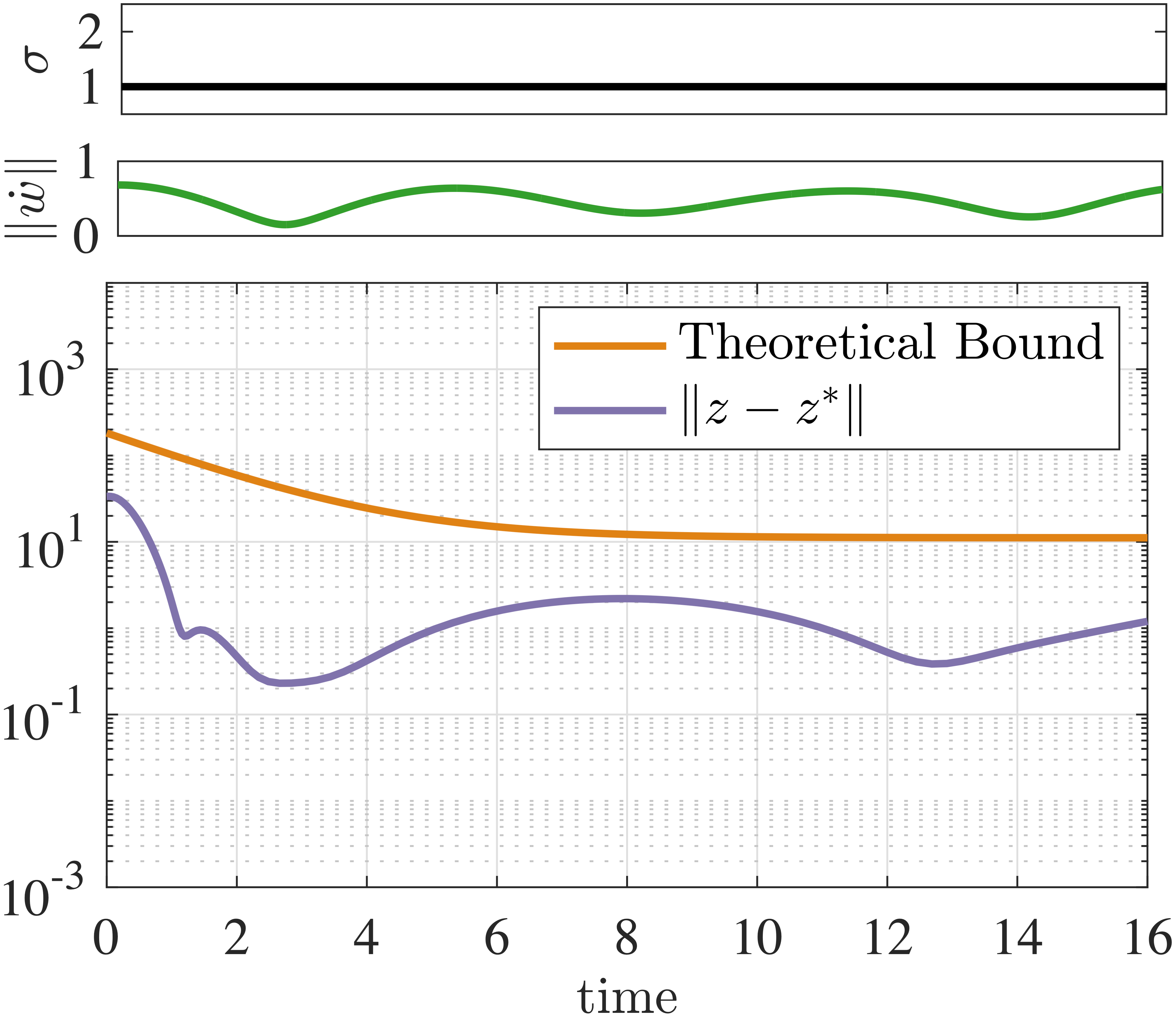
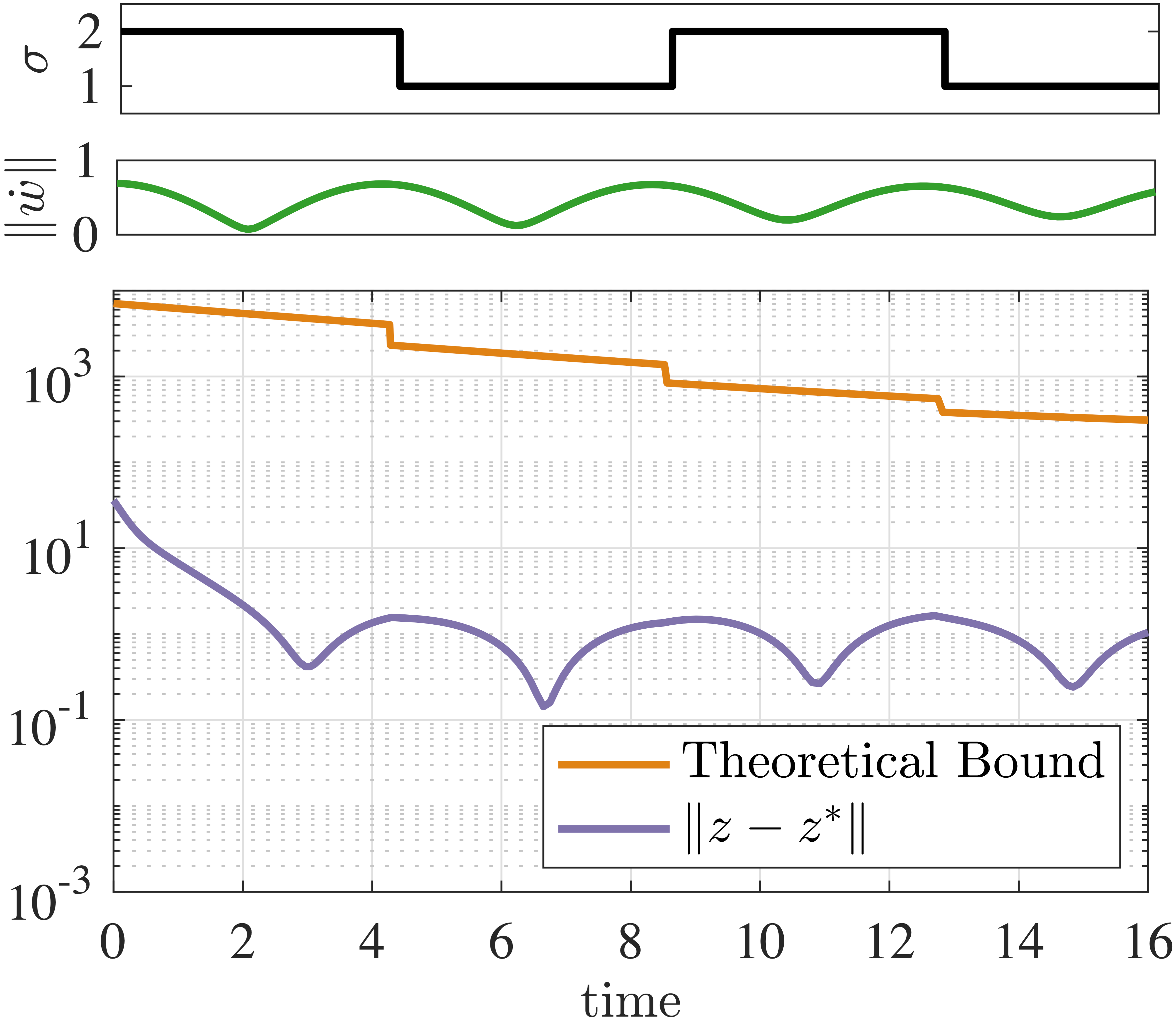
Figure 2: Tracking error of gradient flow controller (10). (a) No plant switching. (b) Plant switches between two modes.

Next, we consider the hybrid accelerated gradient controller of Section 3.2. When the disturbance $\omega_{t}$ is constant and the plant has a single operating mode (i.e. $\sigma=1$) Fig. 3 compares the performance of the hybrid controller versus the gradient-flow controller. Different reset parameters are considered, with $\Delta=0.5,1,5$; we also consider $\Delta=\infty$, corresponding to (4). In the latter case, it can be shown that the trajectories diverge. Similarly, Fig. 4-(a) shows the bound of Theorem 3.3, when $\omega_{t}$ is time-varying and the switching signal $\sigma$ is constant at all times. Fig. 4-(b) considers the case when the switching signal is time-varying.

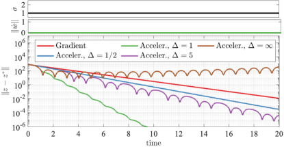
Figure 3: Comparison Gradient Flow vs Accelerated Gradient.

We note that in this simulation the time horizon has been rescaled in order to illustrate the behavior of the controller under switching of the plant.

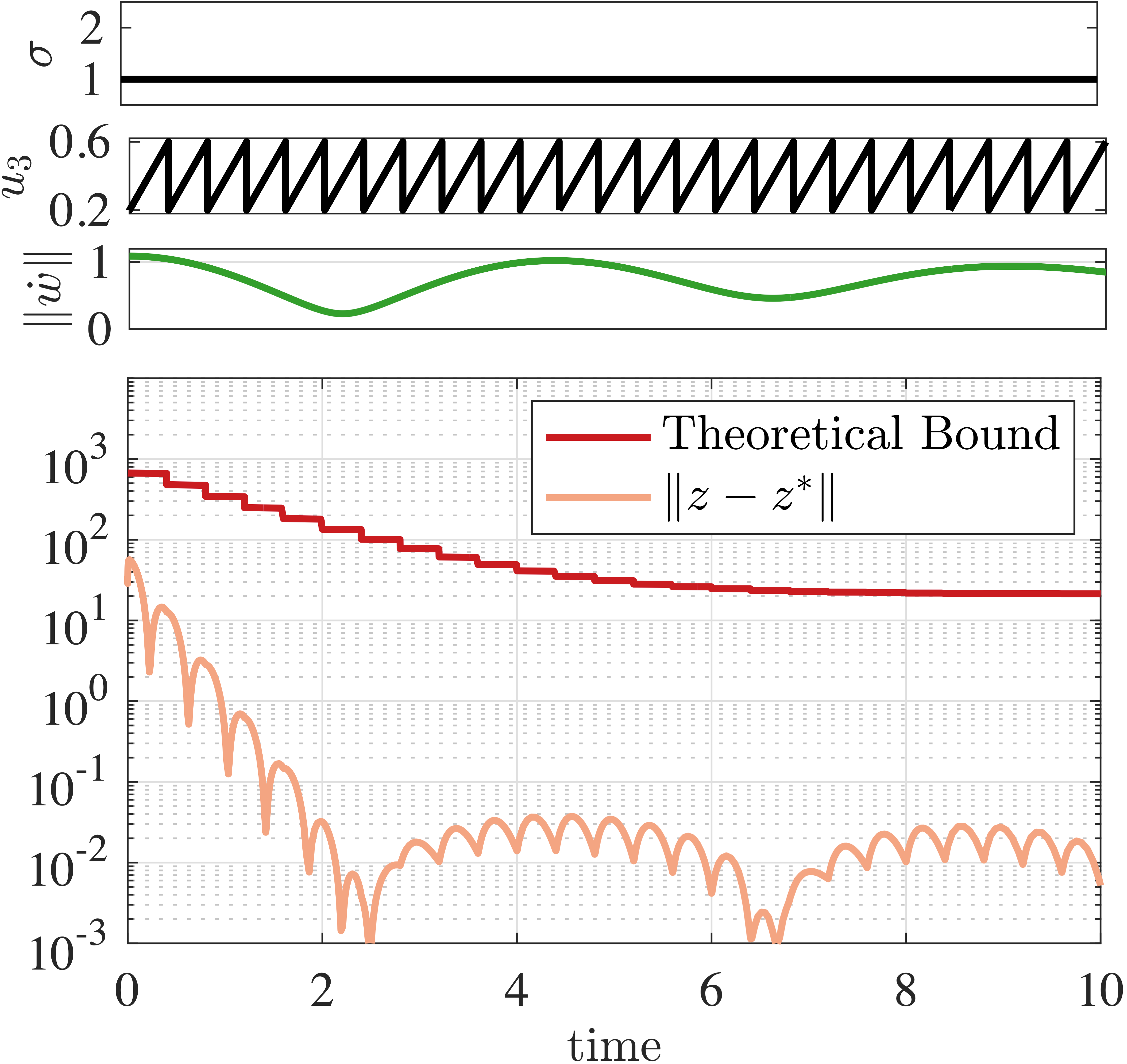
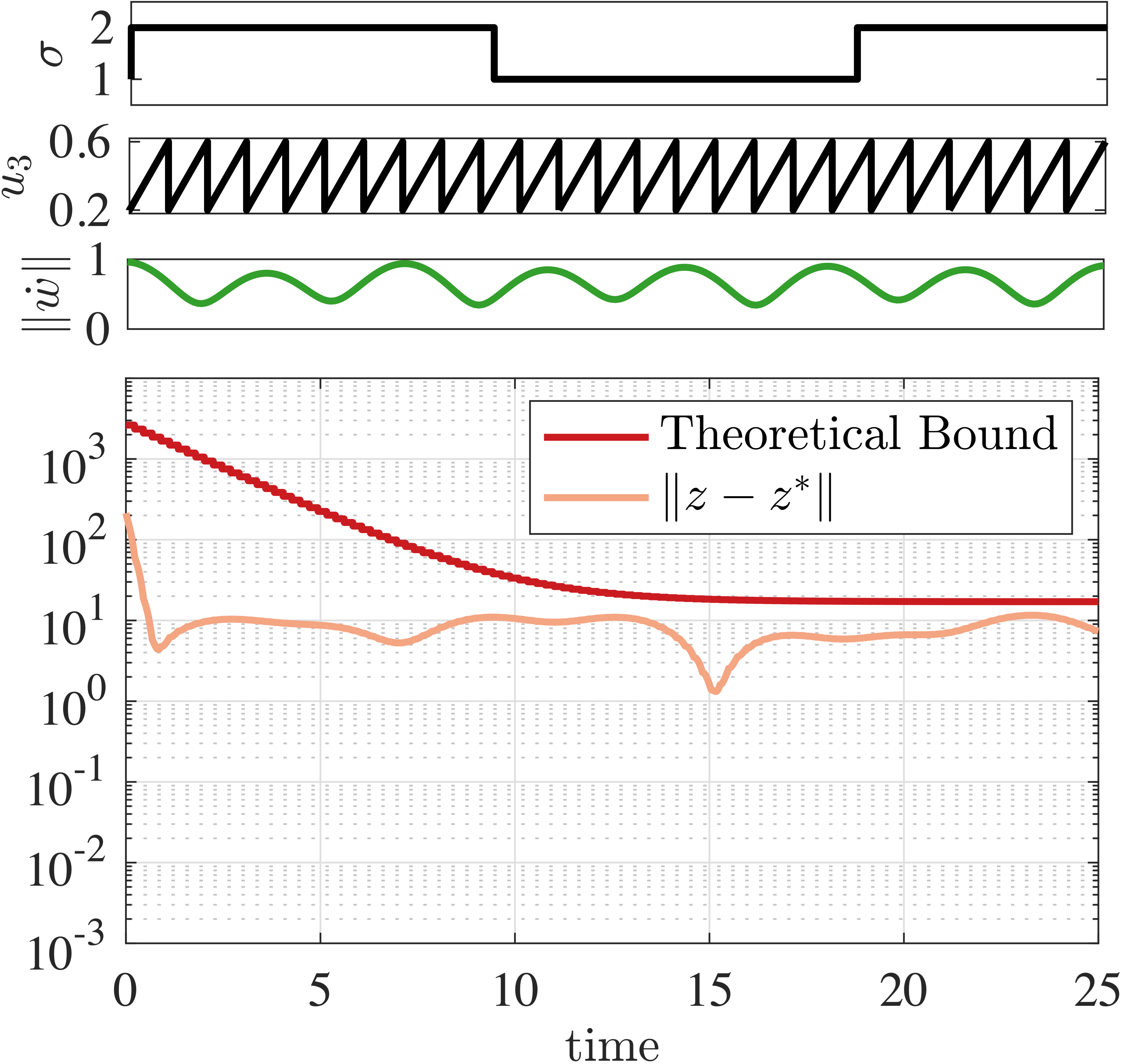
Figure 4: Tracking error of accelerated gradient controller. (a) No plant switching. (b) Switched plant.

Finally, Fig. 5 illustrates the bound in Theorem 3.2. In this case, we consider a scalar plant ($n=m=p=1$) with a single mode ($|\mathcal{S}|=1$) and cost function $\phi_{t}(u)=0.25(Gu+H\omega_{t}-{y}_{\textup{ref}})^{4}$, where ${y}_{\textup{ref}}\in\real$. Note that $\phi_{t}$ satisfies Assumption 6 and Assumption 4 on compact sets. Two important observations follow from Fig. 5. First, the simulations suggest that in this case smaller restarting times $\Delta$ can improve transient performance. Second, the simulation illustrates that the control signal converges only to a neighborhood of the optimal point, thus validating the conclusion of Theorem 3.2. The neighborhood of convergence can be characterized by observing that Assumption 6 implies $(u-{u}_{\textup{ref}})^{2}>\nu_{0}^{2}$, and thus $\nu_{0}^{2}=\ell_{0}$. This condition is illustrated at the top of Fig. 5. Finally, Fig. 5-(c) compares the regulation error of the gradient flow controller versus the hybrid accelerated gradient controller. The figure shows that the accelerated gradient controller achieves faster convergence compared to the gradient descent-based controller, but the convergence is guaranteed only up to a neighborhood of the optimal points.

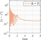
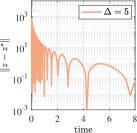
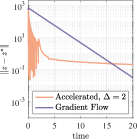
Figure 5: Tracking error of accelerated gradient controller with polynomial cost function. (a) $\Delta=2$. (b) $\Delta=5$. (c) Comparison with Gradient Flow.

6 Conclusions

We addressed the problem of online optimization of switched linear time invariant dynamical systems via optimization-based controllers. We introduced two feedback controllers, one based on gradient descent flows, and a one based on a hybrid regularization of accelerated gradient systems with dynamic momentum. Under a suitable average dwell-time constraint on the switching signal, we established ISS properties for the closed-loop system with input being the time-derivative of the disturbance. This generalizes previous results on time-invariant optimization problems and non-switching plants. Future research directions will focus on developing tighter interconnection bounds between hybrid plants and hybrid controllers via small gain arguments.

References

- [1] F. D. Brunner, H.-B. Dürr, C. Ebenbauer, Feedback design for multi-agent systems: A saddle point approach, in: IEEE Conf. on Decision and Control, 2012, pp. 3783–3789.
- [2] A. Jokic, M. Lazar, P. P. V. D. Bosch, On constrained steady-state regulation: Dynamic KKT controllers, IEEE Transactions on Automatic Control 54 (9) (2009) 2250–2254.
- [3] M. Colombino, E. Dall’Anese, A. Bernstein, Online optimization as a feedback controller: Stability and tracking, IEEE Transactions on Control of Network Systems 7 (1) (2020) 422–432.
- [4] A. Hauswirth, S. Bolognani, G. Hug, F. Dörfler, Timescale separation in autonomous optimization, IEEE Transactions on Automatic Control 66 (2) (2020) 611–624.
- [5] S. Menta, A. Hauswirth, S. Bolognani, G. Hug, F. Dörfler, Stability of dynamic feedback optimization with applications to power systems, in: Annual Conf. on Communication, Control, and Computing, 2018, pp. 136–143.
- [6] L. S. P. Lawrence, Z. E. Nelson, E. Mallada, J. W. Simpson-Porco, Optimal steady-state control for linear time-invariant systems, in: IEEE Conf. on Decision and Control, Miami Beach, FL, USA, 2018, pp. 3251–3257.
- [7] L. S. Lawrence, J. W. Simpson-Porco, E. Mallada, Linear-convex optimal steady-state control, arXiv preprint (2018) arXiv:1810.12892.
- [8] T. Zheng, J. W. Simpson-Porco, E. Mallada, Implicit trajectory planning for feedback linearizable systems: A time-varying optimization approach, arXiv preprint (2019) arXiv:1910.00678.
- [9] G. Bianchin, F. Pasqualetti, Gramian-based optimization for the analysis and control of traffic networks, IEEE Transactions on Intelligent Transportation Systems 21 (7) (2020) 3013–3024.
- [10] H. K. Khalil, Nonlinear Systems, 2nd Edition, Prentice Hall, Upper Saddle River, NJ, 2002.
- [11] R. Goebel, R. G. Sanfelice, A. R. Teel, Hybrid dynamical systems: modeling stability, and robustness, Princeton University Press, Princeton, NJ, 2012.
- [12] J. P. Hespanha, A. S. Morse, Stability of switched systems with average dwell-time, in: IEEE Conf. on Decision and Control, Phoenix, AZ, USA, 1999, pp. 2655–2660.
- [13] A. Wibisono, A. C. Wilson, M. I. Jordan, A variational perspective on accelerated methods in optimization, Proceedings of the National Academy of Sciences 113 (47) (2016) E7351–E7358.
- [14] W. Su, S. Boyd, E. Candes, A differential equation for modeling Nesterov’s accelerated gradient method: Theory and insights, in: Advances in Neural Information Processing Systems 27, Curran Associates, 2014, pp. 2510–2518.
- [15] J. I. Poveda, N. Li, Robust hybrid zero-order optimization algorithms with acceleration via averaging in time, Automatica 123 (2021) 109361.
- [16] J. E. Gaudio, A. M. Annaswamy, M. A. Bolender, E. Lavretsky, A class of high order tuners for adaptive systems, IEEE Control Systems Letters 5 (2) (2021) 391–396.
- [17] B. Shi, S. S. Du, M. I. Jordan, W. J. Su, Understanding the acceleration phenomenon via high-resolution differential equations, Mathematical Programming (Jul 2021).
- [18] J. Zhang, C. A. Uribe, A. Mokhtari, A. Jadbabaie, Achieving acceleration in distributed optimization via direct discretization of the heavy-ball ode, arXiv:1811.02521 (2018).
- [19] J. I. Poveda, N. Li, Inducing uniform asymptotic stability in non-autonomous accelerated optimization dynamics via hybrid regularization, in: IEEE Conf. on Decision and Control, Nice, France, 2019, pp. 3000–3005.
- [20] J. I. Poveda, A. R. Teel, The Heavy-Ball ODE with time-varying damping: Persistence of excitation and uniform asymptotic stability, American Control Conference (2020) 773–778.
- [21] A. R. Teel, L. Moreau, D. Nesic, A unified framework for input-to-state stability in systems with two time scales, IEEE Transactions on Automatic Control (2003) 1526–1544.
- [22] L. Marconi, A. R. Teel, A note about hybrid linear regulation, in: IEEE Conf. on Decision and Control, 2010, pp. 1540–1545.
- [23] V. Gazi, Output regulation of a class of linear systems with switched exosystems, International Journal of Control 80 (10) (2007) 1665–1675.
- [24] P.-A. Absil, K. Kurdyka, On the stable equilibrium points of gradient systems, Systems & Control Letters 55 (7) (2006) 573–577.
- [25] B. O’Donoghue, E. Candes, Adaptive restart for accelerated gradient schemes, Foundations of computational mathematics 15 (3) (2015) 715–732.
- [26] C. Prieur, I. Queinnec, S. Tarbouriech, L. Zaccarian, Analysis and synthesis of reset control systems, Foundations and Trends in Systems and Control 6 (2018) 117–338.