Enhancing photoelectric current by nonclassical light

Abstract

We study the photoelectric current generated by a driving light with nonclassical photon statistics. Due to the nonclassical input photon statistics, it is no longer enough to treat the driving light as a planar wave as in classical physics. We make a quantum approach to study such problems, and find that: when the driving light starts from a coherent state as the initial state, our quantum treatment well returns the quasi-classical driving description; when the the driving light is a generic state with a certain P function, the full system dynamics can be reduced as the P function average of many “branches” – in each dynamics branch, the driving light starts from a coherent state, thus again the system dynamics can be obtained in the above quasi-classical way. Based on this quantum approach, it turns out the different photon statistics does make differences to the photoelectric current. Among all the classical light states with the same light intensity, we prove that the input light with Poisson statistics generates the largest photoelectric current, while a nonclassical sub-Poisson light could exceed this classical upper bound.

Keywords: Nonclassical light, photon statistics, photoelectric current, master equation

1 Introduction

When considering a driving light shining on a quantum two-level system (TLS) ($\hat{H}_{\text{{s}}}=\hbar\Omega|\mathsf{e}\rangle\langle\mathsf{e}|$, with $|\mathsf{e}/\mathsf{g}\rangle$ as the excited/ground state), the interaction between the TLS and the light beam is usually described by the following quasi-classical driving [1, 2, 3],

$$\hat{V}=-\hat{\boldsymbol{d}}\cdot\vec{E}_{0}\sin(\omega_{\mathbf{k}}t-\mathbf{k}\cdot\mathbf{x}-\phi_{0}).$$ (1)

where $\hat{\boldsymbol{d}}=\vec{\wp}\,(\hat{\sigma}^{-}+\hat{\sigma}^{+})$ is the dipole moment operator of the TLS, with $\vec{\wp}:=\langle\mathsf{e}|\hat{\boldsymbol{d}}|\mathsf{g}\rangle$ as the transition dipole moment, and $\hat{\sigma}^{+}:=|\mathsf{e}\rangle\langle\mathsf{g}|=(\hat{\sigma}^{-})^{\dagger}$.

In such an interaction, the driving light is indeed modeled as a planar wave as in classical physics. Thus, if the driving light carries different photon statistics (e.g., Poisson, sub-Poisson, thermal [2, 4, 5, 6, 3]), the above quasi-classical driving interaction cannot reflect this difference.

Recently, it was noticed that the different types of the input photon statistics do exhibit significant features when they interact with the same quantum system. For example, the squeezed light (with sub-Poissonian photon statistics) could enhance the two-photon absorption fluorescence by $\sim 47$ times comparing with the normal laser light with the same intensity [7], and also can be used to exceed the cooling limit in the laser cooling experiments [8, 9, 10], and different nonclassical light states may lead to significant differences in fluorescence spectrum [11] and electron transport [12]. Thus, nonclassical light driving may also bring in potential enhancements in more different physics problems. However, that requires a more precise quantum description for the light-matter interaction beyond the above quasi-classical driving, which has not yet been developed well enough.

In this paper, we make a quantum approach to study the interaction between a quantum system and a driving light, by which the specific photon statistics of the incoming light flux can be taken into account. Based on the interaction between a TLS and the quantized EM field, if the driving mode starts from a coherent state $|\alpha\rangle$ as its initial state, it turns out the system dynamics can be described by a master equation, which just returns the above quasi-classical driving widely adopted in literature.

Further, if the initial state of the driving mode is not a coherent state, but a generic quantum state represented by a P function $\hat{\varrho}=\int d^{2}\alpha\,P(\alpha)|\alpha\rangle\langle\alpha|$, it turns out the system dynamics can be rewritten as the P function average of many evolution “branches”: in each dynamics branch the driving mode starts from a coherent state, thus again it can be solved separately as the above quasi-classical driving situation, and then their P function average gives the full dynamics.

Based on this approach, we study a photoelectric converter model [13, 14, 15, 16, 17, 18, 19], and calculate the photoelectric currents generated by the input light with different photon statistics (Poisson, sub-Poisson, thermal). We find that the photoelectric currents generated from different input photon statistics do exhibit significant differences, even if they have the same light intensity. We prove that, among all the classical light states (those who have non-singular positive P functions [2, 3]), the input light with Poisson statistics generates the largest photoelectric current; on the other hand, the current generated from a nonclassical light with sub-Poisson statistics is even larger than this classical limit.

The paper is arranged as follows. In section 2, we discuss how the quasi-classical approach can be derived from a quantum treatment when the driving light is a coherent state. In section 3, we discuss how to study the system dynamics when the driving light is a generic state. In section 4, we consider a photoelectric converter model and study the photoelectric current by the quasi-classical approach. In section 5, we study the photoelectric current generated by different light states. The summary is drawn in section 6.

2 Quantum treatment of quasi-classical driving

First we show how the above quasi-classical interaction (1) can be derived from a quantum treatment. We start from the general interaction between the TLS and the quantized EM field ($\hat{H}_{\text{{b}}}=\sum_{\mathbf{k},\varsigma}\hbar\omega_{\mathbf{k}}\hat{a}_{\mathbf{k}\varsigma}^{\dagger}\hat{a}_{\mathbf{k}\varsigma}$), which reads (in the interaction picture)

$$\tilde{H}_{\text{{sb}}} = -\tilde{\boldsymbol{d}}(t)\cdot\tilde{\mathbf{E}}(\mathbf{x},t)$$ (2)

$$= -\sum_{\mathbf{k}\varsigma}\tilde{\boldsymbol{d}}(t)\cdot\hat{\mathrm{e}}_{\mathbf{k}\varsigma}\sqrt{\frac{\hbar\omega_{\mathbf{k}}}{2\epsilon_{0}V}}\Big{[}i\hat{a}_{\mathbf{k}\varsigma}e^{i\mathbf{k}\cdot\mathbf{x}-i\omega_{\mathbf{k}}t}+\text{h.c.}\Big{]},$$

where $\varsigma$ is the polarization index of the EM field, and $\mathbf{x}$ is the position of the TLS.

The initial state of the EM field is set as follows: a specific $(\mathbf{k}_{0}\varsigma_{0})$-mode (the driving mode) starts from a coherent state $|\alpha\rangle_{\mathbf{k}_{0}\varsigma_{0}}$ ($\alpha\equiv|\alpha|e^{i\phi_{\alpha}}$), while all the other modes start from the vacuum state, i.e.,

$$\hat{\boldsymbol{\rho}}_{\mathnormal{\textsc{b}}}^{(\alpha)_{\mathbf{k}_{0}\varsigma_{0}}}(0)=\bigotimes_{\mathbf{k}\varsigma}\hat{\varrho}_{\mathbf{k}\varsigma},\qquad\hat{\varrho}_{\mathbf{k}\varsigma}=\cases{|\alpha\rangle\langle\alpha|,&$(\mathbf{k}_{0}\varsigma_{0})$\text{-mode}\\ |0\rangle\langle 0|,&\text{other modes}\\ }$$ (3)

Under this initial state, the field operator $\hat{a}_{\mathbf{k}\varsigma}$ can be divided as its displacement and the vacuum fluctuation $\hat{a}_{\mathbf{k}\varsigma}=\langle\hat{a}_{\mathbf{k}\varsigma}\rangle+\delta\hat{a}_{\mathbf{k}\varsigma}$, namely, the driving mode gives $\hat{a}_{\mathbf{k}_{0}\varsigma_{0}}=\alpha+\delta\hat{a}_{\mathbf{k}_{0}\varsigma_{0}}$ and the other modes give $\hat{a}_{\mathbf{k}\varsigma}=\delta\hat{a}_{\mathbf{k}\varsigma}$. Then the interaction (2) can be rewritten as $\tilde{H}_{\text{{sb}}}=\tilde{V}_{\alpha}(t)+\tilde{H}_{\text{{sb}}}^{(0)}$, where

$$\tilde{V}_{\alpha}(t) = -\tilde{\boldsymbol{d}}(t)\cdot\vec{E}_{\alpha}\sin(\omega_{\mathbf{k}_{0}}t-\mathbf{k}_{0}\cdot\mathbf{x}-\phi_{\alpha}),$$ (4)

$$\tilde{H}_{\text{{sb}}}^{(0)} = -\sum_{\mathbf{k}\varsigma}\tilde{\boldsymbol{d}}(t)\cdot\hat{\mathrm{e}}_{\mathbf{k}\varsigma}\sqrt{\frac{\hbar\omega_{\mathbf{k}}}{2\epsilon_{0}V}}\Big{[}i\,\delta\hat{a}_{\mathbf{k}\varsigma}e^{i\mathbf{k}\cdot\mathbf{x}-i\omega_{\mathbf{k}}t}+\text{h.c.}\Big{]},$$

with $\vec{E}_{\alpha}:=\hat{\mathrm{e}}_{\mathbf{k}_{0}\varsigma_{0}}|\alpha|\sqrt{2\hbar\omega_{\mathbf{k}_{0}}/\epsilon_{0}V}$ (set $\mathbf{x}\equiv 0$ hereafter).

Therefore, $\tilde{V}_{\alpha}(t)$ just gives the above quasi-classical interaction (1) between the TLS and a planar wave. We remark that up to now the above treatments are exact without any rotating-wave approximation (RWA), and it applies for both resonant and non-resonant driving.

On the other hand, in the interaction term $\tilde{H}_{\text{{sb}}}^{(0)}$ of equation (4), $\delta\hat{a}_{\mathbf{k}\varsigma}=\hat{a}_{\mathbf{k}\varsigma}-\langle\hat{a}_{\mathbf{k}\varsigma}\rangle$ only contains the field fluctuation around its mean value, which satisfies $\langle\delta\hat{a}_{\mathbf{k}\varsigma}\rangle=0$, $\langle\delta\hat{a}_{\mathbf{k}\varsigma}\,\delta\hat{a}_{\mathbf{k}^{\prime}\varsigma^{\prime}}^{\dagger}\rangle=\delta_{\mathbf{k}\mathbf{k}^{\prime}}\delta_{\varsigma\varsigma^{\prime}}$, and $\langle\delta\hat{a}_{\mathbf{k}\varsigma}^{\dagger}\delta\hat{a}_{\mathbf{k}^{\prime}\varsigma^{\prime}}^{\dagger}\rangle=\langle\delta\hat{a}_{\mathbf{k}\varsigma}\,\delta\hat{a}_{\mathbf{k}^{\prime}\varsigma^{\prime}}\rangle=0$ for all ($\mathbf{k}\varsigma$)-modes. Notice that these relations and $\tilde{H}_{\text{{sb}}}^{(0)}$ just have the same form as the weak interaction between the TLS and the quantized vacuum field when considering the spontaneous emission. Thus we can apply the Born-Markovian approximation and RWA [20], and obtain the following master equation of the system dynamics (see derivation in A)

$$\partial_{t}\tilde{\rho}_{\text{{s}}}^{(\alpha)} = \frac{i}{\hbar}[\tilde{\rho}_{\text{{s}}}^{(\alpha)},\,\tilde{V}_{\alpha}(t)]+{\cal L}_{\text{{em}}}[\tilde{\rho}_{\text{{s}}}^{(\alpha)}],$$

$${\cal L}_{\text{{em}}}[\rho] = \kappa\big{(}\hat{\sigma}^{-}\rho\hat{\sigma}^{+}-\frac{1}{2}\{\hat{\sigma}^{+}\hat{\sigma}^{-},\,\rho\}\big{)}.$$ (5)

This is just the master equation widely adopted in literature, which contains both the quasi-classical driving and the spontaneous emission term ${\cal L}_{\text{{em}}}[\rho]$ with decay rate $\kappa$. But now the driving term here is no longer directly imposed from the quasi-classical interaction (1) in priori, but emerges from the initial coherent state of the quantized field (3).

3 Driving by generic light states

Now we consider a more general situation that the initial state of the driving mode is not a coherent state but a generic quantum state, while all the other modes still start from the vacuum state.

In this case, such an initial state cannot return the above quasi-classical driving any more. Generally, the initial states of the $(\mathbf{k}_{0}\varsigma_{0})$-mode and the whole EM field can be written in the following P representation [2, 3, 21, 22, 1, 12, 23],

$$\hat{\varrho}_{\mathbf{k}_{0}\varsigma_{0}} = \int d^{2}\alpha\,P(\alpha)\,|\alpha\rangle_{\mathbf{k}_{0}\varsigma_{0}}\langle\alpha|,$$

$$\hat{\boldsymbol{\rho}}_{\mathnormal{\textsc{b}}}(0) = \bigotimes_{\mathbf{k}\varsigma}\,\hat{\varrho}_{\mathbf{k}\varsigma}=\int d^{2}\alpha\,P(\alpha)\,\hat{\boldsymbol{\rho}}_{\mathnormal{\textsc{b}}}^{(\alpha)_{\mathbf{k}_{0}\varsigma_{0}}},$$ (6)

where $\hat{\boldsymbol{\rho}}_{\mathnormal{\textsc{b}}}^{(\alpha)_{\mathbf{k}_{0}\varsigma_{0}}}$ is just given by equation (3). The bath state $\hat{\boldsymbol{\rho}}_{\mathnormal{\textsc{b}}}(0)$ “looks like” a probabilistic collection of many components $\hat{\boldsymbol{\rho}}_{\mathnormal{\textsc{b}}}^{(\alpha)_{\mathbf{k}_{0}\varsigma_{0}}}$, but remember the P function $P(\alpha)$ is not a probability distribution and it may contain negative parts [3, 2, 1].

Now the evolution of the system state $\hat{\rho}_{\text{{s}}}(t)$ can be given by

$$\hat{\rho}_{\mathnormal{\textsc{s}}}(t) = \mathrm{tr}_{\text{{b}}}\Big{\{}\mathcal{E}_{t}[\hat{\rho}_{\mathnormal{\textsc{s}}}(0)\otimes\hat{\boldsymbol{\rho}}_{\mathnormal{\textsc{b}}}(0)]\Big{\}}$$ (7)

$$= \int d^{2}\alpha\,P(\alpha)\,\mathrm{tr}_{\text{{b}}}\Big{\{}\mathcal{E}_{t}[\hat{\rho}_{\mathnormal{\textsc{s}}}(0)\otimes\hat{\boldsymbol{\rho}}_{\mathnormal{\textsc{b}}}^{(\alpha)}(0)]\Big{\}}$$

$$:= \int d^{2}\alpha\,P(\alpha)\,\hat{\rho}_{\text{{s}}}^{(\alpha)}(t),$$

where $\mathcal{E}_{t}[...]$ is the unitary evolution operator of the whole s-b system, and $\hat{\rho}_{\text{{s}}}^{(\alpha)}(t):=\mathrm{tr}_{\text{{b}}}\Big{\{}\mathcal{E}_{t}[\hat{\rho}_{\mathnormal{\textsc{s}}}(0)\otimes\hat{\boldsymbol{\rho}}_{\mathnormal{\textsc{b}}}^{(\alpha)_{\mathbf{k}_{0}\varsigma_{0}}}(0)]\Big{\}}$.

It is worth noting that indeed $\hat{\rho}_{\text{{s}}}^{(\alpha)}(t)$ indicates the system dynamics when the field state starts from $\hat{\boldsymbol{\rho}}_{\mathnormal{\textsc{b}}}^{(\alpha)_{\mathbf{k}_{0}\varsigma_{0}}}(0)$ [equation (3)], which is just the above situation of quasi-classical driving given $|\alpha\rangle$ as the initial state of the $(\mathbf{k}_{0}\varsigma_{0})$-mode.

Therefore, the complete system dynamics $\hat{\rho}_{\mathnormal{\textsc{s}}}(t)$ [equation (7)] can be regarded as the P function average of many evolution “branches” $\hat{\rho}_{\text{{s}}}^{(\alpha)}(t)$, and we call $\hat{\rho}_{\text{{s}}}^{(\alpha)}(t)$ as the $\alpha$-branch of the full dynamics. In each $\alpha$-branch, the driving mode just starts from the coherent state $|\alpha\rangle$ as the initial state, thus, the system dynamics can be regarded as governed by the quasi-classical driving interaction $\tilde{V}_{\alpha}(t)$ and the weak coupling with the quantized vacuum field $\tilde{H}_{\text{{sb}}}^{(0)}$ [equation (4)]. Approximately, $\hat{\rho}_{\mathnormal{\textsc{s}}}(t)$ can be given by the above master equation (5) from Born-Markovian approximation and RWA.

Besides, equation (7) also provides a simple way to obtain the dynamics of system observable expectations, i.e.,

$$\langle\hat{O}_{\mathnormal{\textsc{s}}}(t)\rangle=\mathrm{tr}_{\text{{s}}}\big{[}\hat{O}_{\mathnormal{\textsc{s}}}\,\hat{\rho}_{\text{{s}}}(t)\big{]}=\int d^{2}\alpha\,P(\alpha)\,\langle\hat{O}_{\mathnormal{\textsc{s}}}(t)\rangle^{(\alpha)},$$ (8)

where $\langle\hat{O}_{\mathnormal{\textsc{s}}}(t)\rangle^{(\alpha)}=\mathrm{tr}_{\text{{s}}}[\hat{O}_{\mathnormal{\textsc{s}}}\cdot\hat{\rho}_{\text{{s}}}^{(\alpha)}(t)]$ can be obtained by the master equation (5) with quasi-classical driving.

In sum, if the driving light on the system is not a coherent state, the system dynamics $\langle\hat{O}_{\mathnormal{\textsc{s}}}(t)\rangle$ can be obtained as the P function average of all the branches $\langle\hat{O}_{\mathnormal{\textsc{s}}}(t)\rangle^{(\alpha)}$, and each branch can be given by the master equation (5) with the quasi-classical driving interaction.

We emphasize that, the interaction (4) in each $\alpha$-branch and the P function averages (7, 8) are formally exact, but evaluating the dynamics $\hat{\rho}_{\text{{s}}}^{(\alpha)}(t)$ of each $\alpha$-branch often requires some approximations (e.g., Born-Markovian approximation, and RWA). When the system-bath coupling strength is strong, the backaction from the system to the field could be important; in this case, high-order Markovian corrections can be taken into account in the evaluation of each $\alpha$-branch, and the above P function averages (7, 8) still apply. Throughout this paper, we focus on the situation that the system-bath coupling is quite weak, and quantum effect only comes from the input light state, thus the above Markovian master equation is precise enough for each $\alpha$-branch.

If more than one TLS are concerned, the generalization is straightforward: in each $\alpha$-branch, the interaction between each single TLS with the EM field is still given by the interaction (4), which can be further used to study the field induced interaction between different TLSs [24, 25, 26, 27, 28]. Throughout this paper we only focus on the situation of one TLS, and do not consider the field induced interaction.

4 Photoelectric converter model

Now we consider a photoelectric converter model and study the photoelectric current excited from different light states. The photoelectric converter is modeled as two fermionic levels, $\hat{H}_{\mathnormal{\textsc{s}}}=\hbar\Omega_{a}\hat{a}^{\dagger}\hat{a}+\hbar\Omega_{b}\hat{b}^{\dagger}\hat{b}$ (setting $\Omega_{b}\equiv 0$, and $\Omega_{a}-\Omega_{b}:=\Omega$), and they contact with two electron leads $\hat{H}_{\text{{l}}(\text{{r}})}=\sum_{k}\varepsilon_{\text{{l}}(\text{{r}}),k}\,\hat{c}_{\text{{l}}(\text{{r}}),k}^{\dagger}\hat{c}_{\text{{l}}(\text{{r}}),k}$ respectively via the tunneling interaction $\hat{V}_{\text{{l}}}=\sum_{k}g_{\text{{l}},k}\,\hat{b}^{\dagger}\hat{c}_{\text{{l}},k}+\text{h.c.}$ and $\hat{V}_{\text{{r}}}=\sum_{k}g_{\text{{r}},k}\,\hat{a}^{\dagger}\hat{c}_{\text{{r}},k}+\text{h.c.}$ (see figure 1, here $\hat{a}$, $\hat{b}$, $\hat{c}_{\text{{l}}(\text{{r}}),k}$ are the fermionic annihilation operators of the two levels and the electron modes in the leads). This model has been well used to study photoelectric current generation in a solar cell [14, 15, 16, 17, 18, 29], and the photon-induced electron transport across a molecule junction [13, 30, 31].

In a photoelectric converter made by a p-n diode, the different doping types make the region near the p-n interface lose the electric neutrality and form a depletion layer, and that creates an internal electric field, which makes the diode unidirectional [18]. Thus here the two fermionic levels do not have direct tunneling, and they cannot exchange with each other without the mediation of the EM field. The incoming photons could stimulate the electron up and down, exchanging between these two levels. The interaction between these two fermion levels and the quantized EM field is just the above $\hat{H}_{\text{{sb}}}$ [equation (2)], except here the dipole moment operator should be modified as $\hat{\boldsymbol{d}}=\vec{\wp}(\hat{\tau}^{-}+\hat{\tau}^{+})$ with $\hat{\tau}^{+}:=\hat{a}^{\dagger}\hat{b}=(\hat{\tau}^{-})^{\dagger}$.

Therefore, the above discussions for different input light states can be well applied here. We first consider the situation that the driving light is a coherent state $|\alpha\rangle$ [equation (3)], then the master equation for the system dynamics is obtained as

$$\partial_{t}\tilde{\rho}_{\text{{s}}} = \frac{i}{\hbar}[\tilde{\rho}_{\text{{s}}},\tilde{V}_{\alpha}(t)]+{\cal L}_{\text{{em}}}[\tilde{\rho}_{\text{{s}}}]+{\cal L}_{a}[\tilde{\rho}_{\text{{s}}}]+{\cal L}_{b}[\tilde{\rho}_{\text{{s}}}],$$ (9)

$$\tilde{V}_{\alpha}(t) = i\hbar\xi_{0}\alpha\,\hat{\tau}^{+}e^{i(\Omega-\omega_{\mathbf{k}_{0}})t}-i\hbar\xi_{0}^{*}\alpha^{*}\,\hat{\tau}^{-}e^{-i(\Omega-\omega_{\mathbf{k}_{0}})t}.$$

Here RWA has been applied to the driving interaction $\tilde{V}_{\alpha}(t)$, and $\hbar\xi_{0}:=-(\vec{\wp}\cdot\hat{\mathrm{e}}_{\mathbf{k}_{0}\varsigma_{0}})\sqrt{\hbar\omega_{\mathbf{k}_{0}}/2\epsilon_{0}V}$ is the single-photon coupling strength. Hereafter we only focus on the resonant driving case and set $\omega_{\mathbf{k}_{0}}\equiv\Omega$.

${\cal L}_{\text{{em}}}[\tilde{\rho}_{\text{{s}}}]$ is the same with equation (5) except here $\hat{\sigma}^{\pm}$ should be replaced by $\hat{\tau}^{\pm}$, which describes the spontaneous emission. ${\cal L}_{a(b)}[\tilde{\rho}_{\text{{s}}}]$ describes the dissipation due to coupling with the right (left) lead, which reads (taking $\text{{q}}=a,b$) [17, 32, 13, 33, 16]

$$\mathcal{L}_{\text{{q}}}[\rho] = \gamma_{\text{{q}}}\bar{\mathtt{n}}_{\text{{q}}}(\hat{\text{{q}}}^{\dagger}\rho\hat{\text{{q}}}-\frac{1}{2}\hat{\text{{q}}}\hat{\text{{q}}}^{\dagger}\rho-\frac{1}{2}\rho\hat{\text{{q}}}\hat{\text{{q}}}^{\dagger})$$ (10)

$$+ \gamma_{\text{{q}}}(1-\bar{\mathtt{n}}_{\text{{q}}})(\hat{\text{{q}}}\rho\hat{\text{{q}}}^{\dagger}-\frac{1}{2}\hat{\text{{q}}}^{\dagger}\hat{\text{{q}}}\rho-\frac{1}{2}\rho\hat{\text{{q}}}^{\dagger}\hat{\text{{q}}}),$$

where $\bar{\mathtt{n}}_{a(b)}=\big{[}\exp\beta_{\text{{r(l)}}}(\hbar\Omega_{a(b)}-\mu_{\text{{r(l)}}})+1\big{]}^{-1}$ is the Fermi-Dirac distribution, and $\mu_{\text{{r(l)}}}$ is the chemical potential of the right (left) lead. Here we consider the temperatures of the two electron leads are zero, which gives $\bar{\mathtt{n}}_{b}=1$, $\bar{\mathtt{n}}_{a}=0$.

From the master equation (9), the average electron number $\langle\hat{\text{{n}}}_{a}\rangle:=\langle\hat{a}^{\dagger}\hat{a}\rangle$ on level-$a$ gives

$$\partial_{t}\langle\hat{\text{{n}}}_{a}\rangle = \mathrm{tr}\Big{\{}\frac{i}{\hbar}[\tilde{\rho}_{\mathnormal{\textsc{s}}},\tilde{V}_{\alpha}]\,\hat{\text{{n}}}_{a}+\mathcal{L}_{\mathnormal{\textsc{em}}}[\tilde{\rho}_{\mathnormal{\textsc{s}}}]\,\hat{\text{{n}}}_{a}\Big{\}}+\mathrm{tr}\big{\{}\mathcal{L}_{a}[\tilde{\rho}_{\mathnormal{\textsc{s}}}]\,\hat{\text{{n}}}_{a}\big{\}}$$ (11)

$$:= J_{\text{{em}}}-J_{\text{{r}}}.$$

Here $J_{\text{{r}}}:=-\mathrm{tr}\big{\{}\mathcal{L}_{a}[\tilde{\rho}_{\mathnormal{\textsc{s}}}]\,\hat{\text{{n}}}_{a}\big{\}}$ is the current flowing from level-$a$ to the right lead, and $J_{\text{{em}}}$ is the net exciting rate from level-$b$ to level-$a$. In the steady state $\partial_{t}\langle\hat{\text{{n}}}_{a}\rangle\big{|}_{t\rightarrow\infty}=0$, we have $J_{\text{{em}}}=J_{\text{{r}}}:=J(\alpha)$, and the photoelectric current is $-e\,J_{\text{{r}}}$.

The spontaneous rate is usually much smaller than the tunneling rates $\kappa\ll\gamma_{a,b}:=\gamma$. The above steady state current can be obtained from the master equation (9) [see equation (27) in B]

$$J(\alpha)=\frac{2|\xi_{0}|^{2}\,|\alpha|^{2}\,\gamma}{4|\xi_{0}|^{2}\,|\alpha|^{2}+\gamma^{2}}=\frac{\gamma}{2}\Big{[}1-\frac{\tilde{\gamma}_{\xi}^{2}}{4|\alpha|^{2}+\tilde{\gamma}_{\xi}^{2}}\Big{]},$$ (12)

where $\tilde{\gamma}_{\xi}:=\gamma/|\xi_{0}|$. Thus a non-zero input light ($\alpha\neq 0$) always produces a photoelectric current across the voltage barrier [$J(\alpha)>0$ means the electrons move from left to right].

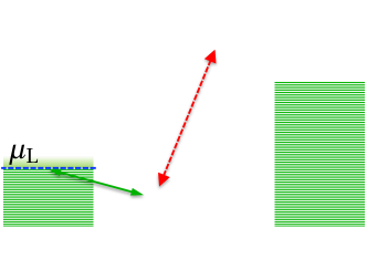
Figure 1: Demonstration of the photoelectric converter model. The fermionic level-$a(b)$ is coupled to the right (left) electron lead, whose chemical potential is $\mu_{\textsc{r}}$ ($\mu_{\text{{l}}}$), and $\hbar\Omega_{a}>\mu_{\text{{r}}}>\mu_{\text{{l}}}>\hbar\Omega_{b}\equiv 0$. The incoming photons excite the electron across the voltage barrier and generate the photoelectric current.

5 Photoelectric current generated by different light states

Now we consider the driving light is not a coherent state, which is beyond the previous quasi-classical description. In this case, equation (12) just gives the steady current for the $\alpha$-branch dynamics, and the complete result should be the summation from all branches [equation (8)], that is, $\overline{J}:=\int d^{2}\alpha\,P(\alpha)J(\alpha)$.

When the light intensity is weak ($|\alpha|^{2}\ll\tilde{\gamma}_{\xi}^{2}\equiv\gamma^{2}/|\xi_{0}|^{2}$), the current equation (12) gives $J(\alpha)\simeq(2|\xi_{0}|^{2}/\gamma)\,|\alpha|^{2}$, thus its P function average always gives the full steady current as $\overline{J}=(2|\xi_{0}|^{2}/\gamma)\,\overline{n}$. That means, the photoelectric current is always proportional to the average photon number $\overline{n}$ (namely, the light intensity) in spite of the input photon statistics. If this weak intensity condition is not satisfied, the photoelectric current may exhibit significant differences for different input light states.

We first consider the input light state is a uniform mixture of all the coherent state $|\alpha\rangle$ with the same photon number $|\alpha|^{2}\equiv\overline{n}$ but different phases $\phi_{\alpha}$, which can be written as $\rho=\int\frac{d\phi_{\alpha}}{2\pi}\,|\alpha\rangle\langle\alpha|=\sum P_{n}|n\rangle\langle n|$, with $P_{n}=e^{-|\alpha|^{2}}|\alpha|^{2n}/n!$ as the Poisson distribution. In this situation (the idealistic laser statistics), the P function average on $J(\alpha)$ gives the same result as equation (12) [solid blue line in figure 2(c, d)].

Now we consider the input light is a monochromatic one carrying the thermal statistics, described by the P function $P_{\text{th}}(\alpha)=[\pi\bar{n}]^{-1}\exp[-|\alpha|^{2}/\bar{n}]$ with $\overline{n}$ as the mean photon number [3, 6, 2, 1]. In this case, the steady current becomes

$$\overline{J}_{\text{th}}=\int d^{2}\alpha\,P_{\text{th}}(\alpha)J(\alpha)=\frac{\gamma}{2}\Big{[}1+\frac{\tilde{\gamma}_{\xi}^{2}}{4\overline{n}}\,e^{\frac{\tilde{\gamma}_{\xi}^{2}}{4\overline{n}}}\mathrm{Ei}(-\frac{\tilde{\gamma}_{\xi}^{2}}{4\overline{n}})\Big{]},$$ (13)

where $\mathrm{Ei}(x):=-\int_{-x}^{\infty}dt\,e^{-t}/t$ is the exponential integral function [chain red line in figure 2(c, d)].

It turns out that, under the same average photon number (light intensity), the currents excited from the Poisson and thermal light exhibit significant differences. The current generated by the Poisson light is always larger than the thermal case [figure 2(c, d)]. Meanwhile, in the weak intensity region ($0<\overline{n}\ll\tilde{\gamma}_{\xi}^{2}$), these two results [equations (12, 13)] almost coincide with each other, and both exhibit a linear dependence on the average photon number $\overline{n}$, which is consistent with the above discussions.

Further, with the help of Lagrangian multipliers, we can prove, among all the classical light states (those who have $P(\alpha)\geq 0$), under the same mean photon number $\overline{n}$, the Poisson input generates the largest photoelectric current $\overline{J}=\int d^{2}\alpha\,P(\alpha)J(\alpha)$ (D). Namely, the photoelectric current generated from the Poisson light sets the upper bound for all classical light states.

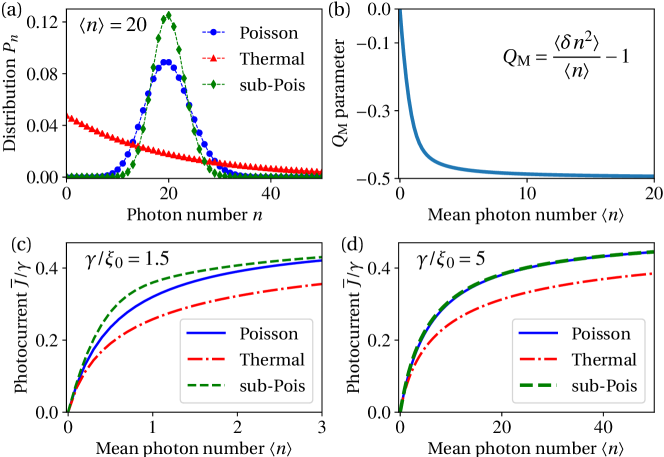
Figure 2: (a) Photon number distribution $P_{n}$ for the thermal, Poisson, sub-Poisson [equation (14)] statistics with the same mean photon number $\overline{n}=20$. (b) The Mandel $Q_{\text{M}}$ parameter for the sub-Poisson distribution [equation (14)] under different mean photon number. (c, d) The photoelectric current $\overline{J}/\gamma$ generated by the Poisson, thermal, sub-Poisson light [equations (12, 13, 15)] (given $\tilde{\gamma}_{\xi}^{2}\equiv\gamma/|\xi_{0}|=1.5,\,5$).

Now we consider the driving light has the following sub-Poisson statistics,

$$P_{n} = \frac{1}{I_{0}(2\sqrt{\lambda})}\frac{\lambda^{n}}{(n!)^{2}},$$

$$\overline{n} = \frac{\sqrt{\lambda}\,I_{1}(2\sqrt{\lambda})}{I_{0}(2\sqrt{\lambda})},\qquad\overline{n^{2}}=\lambda,$$ (14)

where $I_{0/1}(x)$ is the modified Bessel function of the first kind.

The distribution profile is shown in figure 2(a) (green diamonds, for $\overline{n}=20$), and clearly it is narrower than the Poisson distribution with the same average photon number (blue dots). The Mandel $Q_{\text{M}}$ parameter ($Q_{\text{M}}:=\langle\delta n^{2}\rangle/\langle n\rangle-1$) of this distribution is always negative [figure 2(b)], which means such a photon statistics is a nonclassical one, and its P function is not positive-definite [2, 3, 34].

The photoelectric current generated by this sub-Poisson light can be obtained by the P function average of equation (12). Notice that, this P function average is also equivalent with the normal-order expectation on the light state $\rho=\sum P_{n}|n\rangle\langle n|$ [21, 22, 1, 2, 3], namely, $\overline{J}=\langle:J\big{(}\alpha^{*}\rightarrow\hat{a}^{\dagger},\,\alpha\rightarrow\hat{a}\big{)}:\rangle$, where $\langle:J(\hat{a}^{\dagger},\hat{a}):\rangle$ means the normal-order expectation. This can be further calculated with the help of Widder transform [3, 35] (C), which gives the steady state current as

$$\overline{J}_{\text{sub}}=\frac{\gamma}{2}\Big{[}1-\tilde{\gamma}_{\xi}^{2}\int_{0}^{\infty}ds\,e^{-\tilde{\gamma}_{\xi}^{2}s}\,\frac{I_{0}(2\sqrt{(1-4s)\lambda})}{I_{0}(2\sqrt{\lambda})}\Big{]}.$$ (15)

The photoelectric current generated by such a sub-Poisson light is shown in figure 2(c, d) (dashed green line), and it is larger than the above classical upper bound set by the Poisson light. Notice that the surpassing amount is dependent on the tunneling rate $\gamma$ comparing with the single-photon coupling strength $\xi_{0}$. In most practical situations $\gamma\gg|\xi_{0}|$, this difference is quite small [figure 2(d)]. If the tunneling rate is small ($\gamma\sim\xi_{0}$), such a difference due to the input photon statistics could be significant. On the other hand, the difference between the currents generated by the thermal and Poisson light appears independent on $\gamma/|\xi_{0}|\equiv\tilde{\gamma}_{\xi}$ [indeed in both equations (12, 13), $\overline{n}/\tilde{\gamma}_{\xi}^{2}$ appears together as a whole].

It is known that the Poissonian distribution indicates the photons are arriving randomly, while the sub-Poisson light exhibits the anti-bunching effect, indicating the photons are arriving more “regularly” than completely random [2, 1, 3], which leads to the above enhancement. Clearly, nonclassical states are a much larger set than the classical ones, and anti-bunching is just one particular kind of quantum features, thus it is possible that different kinds of nonclassical light may lead to some other novel effects.

6 Summary

In this paper, we made a quantum approach to study photoelectric current generated by a monochromatic driving light which carries a generic photon statistics. If the driving mode starts from a coherent state as the initial state, our quantum treatment just returns the quasi-classical driving description as widely adopted in literature. But if the driving light has a generic photon statistics with a given P function, the full system dynamics becomes the P function average of many evolution “branches”: in each dynamics branch, the driving mode starts from a coherent state and thus returns the quasi-classical driving. Based on this quantum approach, it turns out, different types of photon statistics do make differences to the photoelectric current generation. Among all the classical light states with the same mean photon number, the Poisson statistics generates the largest photoelectric current, while a nonclassical sub-Poisson light could even exceed this classical upper bound. The sub-Poissonian driving light may be realized by the squeezed light or sub-Poissonian laser [36, 37, 38, 39]. The model here has been used to study the photon-induced electron transport in quantum dots [15, 40] and molecule junctions [13, 30, 31]. In principle the above novel results in our study could be observable in these platform when the tunneling rate $\gamma$ is small enough. Meanwhile, it is expectable that some other quantum states which may lead to stronger enhancement in such electronic transport systems, and this approach also can be applied in more different problems with light driving.

Appendix A Master equation derivation

Here we present the derivation for the the master equation (5) in the main text. Since the EM field starts from $\hat{\boldsymbol{\rho}}_{\mathnormal{\textsc{b}}}^{(\alpha)_{\mathbf{k}_{0}\varsigma_{0}}}(0)$ [equation (3) in the main text], in the interaction picture, the interaction between the two-level system and the EM field can be rewritten as $\tilde{H}_{\text{{sb}}}=\tilde{V}_{\alpha}(t)+\tilde{H}_{\text{{sb}}}^{(0)}$ [equation (4) in the main text], where $\tilde{V}_{\alpha}(t)=-\tilde{\boldsymbol{d}}(t)\cdot\vec{E}_{\alpha}\sin(\omega_{\mathbf{k}_{0}}t-\mathbf{k}_{0}\cdot\mathbf{x}-\phi_{\alpha})$, and

$$\tilde{H}_{\text{{sb}}}^{(0)} =-\sum_{\mathbf{k},\varsigma} \big{(}\hat{\sigma}^{-}e^{-i\Omega t}+\hat{\sigma}^{+}e^{i\Omega t}\big{)}\cdot$$ (16)

$$(\vec{\wp}\cdot\hat{\mathrm{e}}_{\mathbf{k}\varsigma})\sqrt{\frac{\hbar\omega_{\mathbf{k}}}{2\epsilon_{0}V}}\Big{[}i\,\delta\hat{a}_{\mathbf{k}\varsigma}\,e^{i\mathbf{k}\cdot\mathbf{x}-i\omega_{\mathbf{k}}t}+\text{h.c.}\Big{]}.$$

Here $\hat{\sigma}^{+}=|\mathsf{e}\rangle\langle\mathsf{g}|=(\hat{\sigma}^{-})^{\dagger}$, and $\tilde{\boldsymbol{d}}(t)=\vec{\wp}(\hat{\sigma}^{-}e^{-i\Omega t}+\text{h.c.})$. The operator $\delta\hat{a}_{\mathbf{k}\varsigma}=\hat{a}_{\mathbf{k}\varsigma}-\langle\hat{a}_{\mathbf{k}\varsigma}\rangle$ indicates the pure fluctuation of the quantized field, and the displacement $\langle\hat{a}_{\mathbf{k}\varsigma}\rangle=\mathrm{tr}_{\text{{b}}}[\hat{\boldsymbol{\rho}}_{\mathnormal{\textsc{b}}}^{(\alpha)_{\mathbf{k}_{0}\varsigma_{0}}}(0)\,\hat{a}_{\mathbf{k}\varsigma}]$ gives $\alpha$ for ($\mathbf{k}_{0}\varsigma_{0}$)-mode and 0 for other modes. Under the rotating-wave approximation, the above interaction becomes

$$\tilde{H}_{\text{{sb}}}^{(0)}(t)\simeq\sum_{\mathbf{k},\varsigma}g_{\mathbf{k}\varsigma}\,\hat{\sigma}^{+}\,\delta\hat{a}_{\mathbf{k}\varsigma}\,e^{i(\Omega-\omega_{\mathbf{k}})t}+\text{h.c.}$$ (17)

where $g_{\mathbf{k}\varsigma}:=-i(\vec{\wp}\cdot\hat{\mathrm{e}}_{\mathbf{k}\varsigma})\sqrt{\hbar\omega_{\mathbf{k}}/2\epsilon_{0}V}\,e^{i\mathbf{k}\cdot\mathbf{x}}$.

In the interaction picture, the dynamics of the system-bath state $\tilde{\boldsymbol{\rho}}_{\text{{sb}}}(t)$ is governed by the von Neumann equation,

$$\partial_{t}\tilde{\boldsymbol{\rho}}_{\text{{sb}}}(t) = \frac{i}{\hbar}[\tilde{\boldsymbol{\rho}}_{\text{{sb}}}(t),\,\tilde{V}_{\alpha}(t)]+\frac{i}{\hbar}[\tilde{\boldsymbol{\rho}}_{\text{{sb}}}(t),\,\tilde{H}_{\text{{sb}}}^{(0)}(t)],$$

$$\tilde{\boldsymbol{\rho}}_{\text{{sb}}}(t) = \tilde{\boldsymbol{\rho}}_{\text{{sb}}}(0)+\frac{i}{\hbar}\int_{0}^{t}ds\,[\tilde{\boldsymbol{\rho}}_{\text{{sb}}}(s),\,\tilde{V}_{\alpha}(s)+\tilde{H}_{\text{{sb}}}^{(0)}(s)].$$ (18)

We put the above integral solution of $\tilde{\boldsymbol{\rho}}_{\text{{sb}}}(t)$ back into the second term of the von Neumann equation, which gives

$$\partial_{t}\tilde{\boldsymbol{\rho}}_{\text{{sb}}}(t) = \frac{i}{\hbar}[\tilde{\boldsymbol{\rho}}_{\text{{sb}}}(t),\,\tilde{V}_{\alpha}(t)]+\frac{i}{\hbar}[\tilde{\boldsymbol{\rho}}_{\text{{sb}}}(0),\,\tilde{H}_{\text{{sb}}}^{(0)}(t)]$$ (19)

$$- \frac{1}{\hbar^{2}}\int_{0}^{t}ds\,\Big{[}[\tilde{\boldsymbol{\rho}}_{\text{{sb}}}(s),\,\tilde{V}_{\alpha}(s)+\tilde{H}_{\text{{sb}}}^{(0)}(s)],\,\tilde{H}_{\text{{sb}}}^{(0)}(t)\Big{]}.$$

Now we apply the Born approximation $\tilde{\boldsymbol{\rho}}_{\text{{sb}}}(s)\simeq\tilde{\rho}_{\text{{s}}}(s)\otimes\hat{\boldsymbol{\rho}}_{\mathnormal{\textsc{b}}}^{(\alpha)_{\mathbf{k}_{0}\varsigma_{0}}}(0)$, and trace out the bath degree of freedom. Since $\langle\delta\hat{a}_{\mathbf{k}\varsigma}\rangle=\langle\delta\hat{a}_{\mathbf{k}\varsigma}^{\dagger}\rangle=0$ under the bath state $\hat{\boldsymbol{\rho}}_{\mathnormal{\textsc{b}}}^{(\alpha)_{\mathbf{k}_{0}\varsigma_{0}}}(0)$, equation (19) further gives

$$\partial_{t}\tilde{\rho}_{\text{{s}}}\simeq\frac{i}{\hbar}[\tilde{\rho}_{\text{{s}}}(t),\,\tilde{V}_{\alpha}(t)]$$

$$-\frac{1}{\hbar^{2}}\int_{0}^{t}ds\,\mathrm{Tr}_{\text{{b}}}\Big{[}[\tilde{\rho}_{\text{{s}}}(t-s)\otimes\hat{\boldsymbol{\rho}}_{\mathnormal{\textsc{b}}}^{(\alpha)_{\mathbf{k}_{0}\varsigma_{0}}}(0),\,\tilde{H}_{\text{{sb}}}^{(0)}(t-s)],\,\tilde{H}_{\text{{sb}}}^{(0)}(t)\Big{]}.$$ (20)

Then we assume the convolution kernel, which comes from the time correlation function of the EM field, decays so fast that only the accumulation around $\tilde{\rho}_{\text{{s}}}(t-s\simeq t)$ dominates in the integral. Thus, we can extend the above time integral to be $t\rightarrow\infty$ (Markovian approximation), and obtain

$$\partial_{t}\tilde{\rho}_{\text{{s}}}\simeq\frac{i}{\hbar}[\tilde{\rho}_{\text{{s}}}(t),\,\tilde{V}_{\alpha}(t)]$$

$$-\frac{1}{\hbar^{2}}\int_{0}^{\infty}ds\,\mathrm{Tr}_{\text{{b}}}\Big{[}[\tilde{\rho}_{\text{{s}}}(t)\otimes\hat{\boldsymbol{\rho}}_{\mathnormal{\textsc{b}}}^{(\alpha)_{\mathbf{k}_{0}\varsigma_{0}}}(0),\,\tilde{H}_{\text{{sb}}}^{(0)}(t-s)],\,\tilde{H}_{\text{{sb}}}^{(0)}(t)\Big{]}.$$ (21)

The master equation can be obtained after taking the trace expectation and time integral. Notice that, when taking the average on the bath state $\hat{\boldsymbol{\rho}}_{\mathnormal{\textsc{b}}}^{(\alpha)_{\mathbf{k}_{0}\varsigma_{0}}}(0)$, the bath operators $\delta\hat{a}_{\mathbf{k}\varsigma}^{\dagger}$ in $\tilde{H}_{\text{{sb}}}^{(0)}(t)$ satisfy the following relations,

$$\langle\delta\hat{a}_{\mathbf{k}\varsigma}^{\dagger}\,\delta\hat{a}_{\mathbf{k}^{\prime}\varsigma^{\prime}}\rangle = 0,\quad\langle\delta\hat{a}_{\mathbf{k}\varsigma}\,\delta\hat{a}_{\mathbf{k}^{\prime}\varsigma^{\prime}}^{\dagger}\rangle=\delta_{\mathbf{k}\mathbf{k}^{\prime}}\delta_{\varsigma\varsigma^{\prime}},$$

$$\langle\delta\hat{a}_{\mathbf{k}\varsigma}\,\delta\hat{a}_{\mathbf{k}^{\prime}\varsigma^{\prime}}\rangle = \langle\delta\hat{a}_{\mathbf{k}\varsigma}^{\dagger}\,\delta\hat{a}_{\mathbf{k}^{\prime}\varsigma^{\prime}}^{\dagger}\rangle=0.$$ (22)

Here we present the calculation of one term in equation (21):

$$-\frac{1}{\hbar^{2}}\int_{0}^{\infty}ds\,\mathrm{Tr}_{\text{{b}}}\Big{[}\tilde{\rho}_{\text{{s}}}(t)\otimes\hat{\boldsymbol{\rho}}_{\mathnormal{\textsc{b}}}^{(\alpha)_{\mathbf{k}_{0}\varsigma_{0}}}(0)\cdot\Big{(}\sum_{\mathbf{k}\varsigma}g_{\mathbf{k}\varsigma}\hat{\sigma}^{+}\delta\hat{a}_{\mathbf{k}\varsigma}\,e^{i(\Omega-\omega_{\mathbf{k}})(t-s)}\Big{)}$$

$$\qquad\cdot\Big{(}\sum_{\mathbf{k}^{\prime}\varsigma^{\prime}}g_{\mathbf{k}^{\prime}\varsigma^{\prime}}^{*}\hat{\sigma}^{-}\delta\hat{a}_{\mathbf{k}^{\prime}\varsigma^{\prime}}^{\dagger}\,e^{-i(\Omega-\omega_{\mathbf{k}^{\prime}})t}\Big{)}\Big{]}$$

$$=-\tilde{\rho}_{\text{{s}}}\hat{\sigma}^{+}\hat{\sigma}^{-}\,\sum_{\mathbf{k}\varsigma}\frac{|g_{\mathbf{k}\varsigma}|^{2}}{\hbar^{2}}\int_{0}^{\infty}ds\,\langle\delta\hat{a}_{\mathbf{k}\varsigma}\delta\hat{a}_{\mathbf{k}\varsigma}^{\dagger}\rangle e^{-i(\Omega-\omega_{\mathbf{k}})s}$$

$$=-\tilde{\rho}_{\text{{s}}}\hat{\sigma}^{+}\hat{\sigma}^{-}\int_{0}^{\infty}\frac{d\omega}{2\pi}\,\Gamma(\omega)\int_{0}^{\infty}ds\,e^{-i(\Omega-\omega)s}$$

$$=-\tilde{\rho}_{\text{{s}}}\hat{\sigma}^{+}\hat{\sigma}^{-}\int_{0}^{\infty}\frac{d\omega}{2\pi}\,\Gamma(\omega)[\pi\delta(\Omega-\omega)-i\mathbf{P}\frac{1}{\Omega-\omega}]$$

$$\simeq-\frac{1}{2}\Gamma(\Omega)\,\tilde{\rho}_{\text{{s}}}\hat{\sigma}^{+}\hat{\sigma}^{-}.$$ (23)

Here the principal integral is omitted, and $\Gamma(\omega):=\frac{2\pi}{\hbar^{2}}\sum_{\mathbf{k}\varsigma}|g_{\mathbf{k}\varsigma}|^{2}\delta(\omega-\omega_{\mathbf{k}\varsigma})$ is the coupling spectral density.

Notice that, when considering the spontaneous emission of the TLS in the vacuum field (without the driving light), the coupling spectral density $\Gamma(\omega)$ is exactly the same with the one used here. Finally, the master equation is obtained as

$$\partial_{t}\tilde{\rho}_{\text{{s}}}=\frac{i}{\hbar}[\tilde{\rho}_{\text{{s}}},\tilde{V}_{\alpha}(t)]+\kappa\big{(}\hat{\sigma}^{-}\tilde{\rho}_{\text{s}}\hat{\sigma}^{+}-\frac{1}{2}\{\hat{\sigma}^{+}\hat{\sigma}^{-},\,\tilde{\rho}_{\text{{s}}}\}\big{)}.$$ (24)

The first term just has the form of quasi-classical driving widely adopted in literature, and second term describes the spontaneous emission with $\kappa:=\Gamma(\Omega)$ as the decay rate.

Appendix B Photoelectric current

Based on the master equation equation (9) in the main text, we obtain the following the equations of motion for the observables $\hat{\text{{n}}}_{a}=\hat{a}^{\dagger}\hat{a}$, $\hat{\text{{n}}}_{b}=\hat{b}^{\dagger}\hat{b}$, and $\hat{\tau}^{+}=\hat{a}^{\dagger}\hat{b}=(\hat{\tau}^{-})^{\dagger}$,

$$\partial_{t}\langle\hat{\text{{n}}}_{a}\rangle=\big{(}\xi_{0}\alpha\langle\hat{\tau}^{+}\rangle+\xi_{0}^{*}\alpha^{*}\langle\hat{\tau}^{-}\rangle\big{)}-\gamma_{a}[(1-\bar{\mathtt{n}}_{a})\langle\hat{\text{{n}}}_{a}\rangle-\bar{\mathtt{n}}_{a}(1-\langle\hat{\text{{n}}}_{a}\rangle)]-\kappa\langle\hat{\text{{n}}}_{a}\rangle,$$

$$\partial_{t}\langle\hat{\text{{n}}}_{b}\rangle=-\big{(}\xi_{0}\alpha\langle\hat{\tau}^{+}\rangle+\xi_{0}^{*}\alpha^{*}\langle\hat{\tau}^{-}\rangle\big{)}-\gamma_{b}[(1-\bar{\mathtt{n}}_{b})\langle\hat{\text{{n}}}_{b}\rangle-\bar{\mathtt{n}}_{b}(1-\langle\hat{\text{{n}}}_{b}\rangle)]+\kappa\langle\hat{\text{{n}}}_{a}\rangle,$$

$$\partial_{t}\langle\hat{\tau}^{+}\rangle=-\xi_{0}^{*}\alpha^{*}\big{(}\langle\hat{\text{{n}}}_{a}\rangle-\langle\hat{\text{{n}}}_{b}\rangle\big{)}-\frac{1}{2}(\gamma_{a}+\gamma_{b}+\kappa)\langle\hat{\tau}^{+}\rangle,$$

$$\partial_{t}\langle\hat{\tau}^{-}\rangle=-\xi_{0}\alpha\big{(}\langle\hat{\text{{n}}}_{a}\rangle-\langle\hat{\text{{n}}}_{b}\rangle\big{)}-\frac{1}{2}(\gamma_{a}+\gamma_{b}+\kappa)\langle\hat{\tau}^{-}\rangle.$$ (25)

In the steady state $t\rightarrow\infty$, the time-derivatives all give zero, and the above algebra equations give the steady state as

$$\langle\hat{\text{{n}}}_{a}\rangle=\frac{4|\alpha|^{2}|\xi_{0}|^{2}(\gamma_{a}\bar{\mathtt{n}}_{a}+\gamma_{b}\bar{\mathtt{n}}_{b})+\gamma_{a}\gamma_{b}(\gamma_{a}+\gamma_{b}+\kappa)\bar{\mathtt{n}}_{a}}{4|\alpha|^{2}|\xi_{0}|^{2}(\gamma_{a}+\gamma_{b})+\gamma_{b}(\gamma_{a}+\kappa)(\gamma_{a}+\gamma_{b}+\kappa)},$$

$$\langle\hat{\text{{n}}}_{b}\rangle=\frac{4|\alpha|^{2}|\xi_{0}|^{2}(\gamma_{a}\bar{\mathtt{n}}_{a}+\gamma_{b}\bar{\mathtt{n}}_{b})+(\gamma_{a}+\gamma_{b}+\kappa)[\kappa\gamma_{a}\bar{\mathtt{n}}_{a}+(\kappa+\gamma_{a})\gamma_{b}\bar{\mathtt{n}}_{b}]}{4|\alpha|^{2}|\xi_{0}|^{2}(\gamma_{a}+\gamma_{b})+\gamma_{b}(\gamma_{a}+\kappa)(\gamma_{a}+\gamma_{b}+\kappa)},$$ (26)

$$\langle\hat{\tau}^{+}\rangle=\langle\hat{\tau}^{-}\rangle^{*}=\frac{2\xi_{0}^{*}\alpha^{*}[\gamma_{a}\gamma_{b}(\bar{\mathtt{n}}_{b}-\bar{\mathtt{n}}_{a})+\kappa(\gamma_{a}\bar{\mathtt{n}}_{a}+\gamma_{b}\bar{\mathtt{n}}_{b})]}{4|\alpha|^{2}|\xi_{0}|^{2}(\gamma_{a}+\gamma_{b})+\gamma_{b}(\gamma_{a}+\kappa)(\gamma_{a}+\gamma_{b}+\kappa)}.$$

Then the electron current flowing to the right electron lead is given by

$$J_{\text{{r}}} = -\mathrm{tr}\Big{\{}{\cal L}_{a}[\tilde{\rho}_{\text{{s}}}]\cdot\hat{\text{{n}}}_{a}\Big{\}}=\gamma_{a}[(1-\bar{\mathtt{n}}_{a})\langle\hat{\text{{n}}}_{a}\rangle-\bar{\mathtt{n}}_{a}(1-\langle\hat{\text{{n}}}_{a}\rangle)]$$ (27)

$$= \frac{4|\alpha|^{2}\,|\xi_{0}|^{2}\gamma_{a}\gamma_{b}(\bar{\mathtt{n}}_{b}-\bar{\mathtt{n}}_{a})-\kappa\gamma_{a}\gamma_{b}(\gamma_{a}+\gamma_{b}+\kappa)\bar{\mathtt{n}}_{a}}{4|\alpha|^{2}|\xi_{0}|^{2}(\gamma_{a}+\gamma_{b})+\gamma_{b}(\gamma_{a}+\kappa)(\gamma_{a}+\gamma_{b}+\kappa)}.$$

Taking $\gamma_{a}=\gamma_{b}:=\gamma$, $\kappa=0$, $\bar{\mathtt{n}}_{a}=0$, $\bar{\mathtt{n}}_{b}=1$, it gives the result (12) in the main text.

Notice that, the second term started with $(-\kappa)$ in the above numerator indeed indicates the electron tunneling from level-a to level-b under the mediation of spontaneous emission, and it still exists when there is no driving light ($\alpha\rightarrow 0$). In this paper, we neglect this effect since the spontaneous rate $\kappa$ is usually much smaller than the tunneling rates $\gamma_{a,b}$.

Appendix C General input photon statistics

Here we show how to calculate the photoelectric current when the input light is not a coherent state but has a general photon statistics. Generally, the P function average of equation (12) in the main text gives the photoelectric current. But for many nonclassical light states, their P functions are highly singular and sometimes not easy to be given directly. Thus here we provide another method to calculate this current. Notice that the P function average is also equivalent as the normal-order expectation on the quantum state $\rho=\int d^{2}\alpha\,P(\alpha)|\alpha\rangle\langle\alpha|$, thus we have (denoting $\tilde{\gamma}_{\xi}:=\gamma/|\xi_{0}|$)

$$\overline{J} = \int d^{2}\alpha\,P(\alpha)\,\frac{2|\xi_{0}|^{2}\gamma\,|\alpha|^{2}}{4|\xi_{0}|^{2}\,|\alpha|^{2}+\gamma^{2}}=\frac{\gamma}{2}-\frac{\gamma}{2}\big{\langle}:\frac{\tilde{\gamma}_{\xi}^{2}}{4\hat{a}^{\dagger}\hat{a}+\tilde{\gamma}_{\xi}^{2}}:\big{\rangle}$$ (28)

$$= \frac{\gamma}{2}\Big{(}1-\tilde{\gamma}_{\xi}^{2}\big{\langle}:\int_{0}^{\infty}ds\,e^{-s(4\hat{a}^{\dagger}\hat{a}+\tilde{\gamma}_{\xi}^{2})}:\big{\rangle}\Big{)}.$$

Here $\langle:f(\hat{a},\hat{a}^{\dagger}):\rangle$ means the normal-order expectation, and the second line is the Widder transform which turns the operator fraction into an exponential integral. Thus, for an arbitrary quantum state $\rho=\sum_{mn}\rho_{mn}|m\rangle\langle n|$, we have

$$\langle:e^{-4s\hat{a}^{\dagger}\hat{a}}:\rangle = \sum_{k=0}^{\infty}\frac{(-4s)^{k}}{k!}\langle(\hat{a}^{\dagger})^{k}\hat{a}^{k}\rangle=\sum_{m,n=0}^{\infty}\sum_{k=0}^{\infty}\rho_{mn}\cdot\frac{(-4s)^{k}}{k!}\langle n|(\hat{a}^{\dagger})^{k}\hat{a}^{k}|m\rangle$$ (29)

$$= \sum_{n=0}^{\infty}\sum_{k=0}^{n}\rho_{nn}\cdot\frac{(-4s)^{k}n!}{k!(n-k)!}=\sum_{n}\rho_{nn}(1-4s)^{n}.$$

Indeed here $\rho_{nn}:=P_{n}$ is just the photon statistics of the input light state, and the above photoelectric current becomes

$$\overline{J}=\frac{\gamma}{2}\Big{(}1-\tilde{\gamma}_{\xi}^{2}\int_{0}^{\infty}ds\,e^{-\tilde{\gamma}_{\xi}^{2}s}\big{[}\sum_{n}P_{n}(1-4s)^{n}\big{]}\Big{)}.$$ (30)

For example, considering the coherent state $|\alpha\rangle$ as the input light, which has $P_{n}=e^{-|\alpha|^{2}}|\alpha|^{2n}/n!$, then equation (30) gives the photoelectric current by

$$\overline{J} = \frac{\gamma}{2}\Big{(}1-\tilde{\gamma}_{\xi}^{2}\int_{0}^{\infty}ds\,e^{-\tilde{\gamma}_{\xi}^{2}s}\big{[}\sum_{n}e^{-|\alpha|^{2}}\frac{|\alpha|^{2n}(1-4s)^{n}}{n!}\big{]}\Big{)}$$ (31)

$$= \frac{\gamma}{2}\Big{(}1-\tilde{\gamma}_{\xi}^{2}\int_{0}^{\infty}ds\,e^{-\tilde{\gamma}_{\xi}^{2}s}\,e^{-4|\alpha|^{2}s}\Big{)}=\frac{\gamma}{2}\Big{[}1-\frac{\tilde{\gamma}_{\xi}^{2}}{4|\alpha|^{2}+\tilde{\gamma}_{\xi}^{2}}\Big{]}.$$

which just returns the result $J(\alpha)$ [equation (12) in the main text]. If we consider the input light is the thermal state $P_{n}=\frac{1}{\bar{n}+1}\big{[}\frac{\bar{n}}{\bar{n}+1}\big{]}^{n}$, the above equation (30) also gives the same result as equation (13) in the main text. If the input light has a sub-Poisson statistics $P_{n}=[I_{0}(2\sqrt{\lambda})]^{-1}\,\lambda^{n}/(n!)^{2}$, the above equation (30) gives the result (15) in the main text.

Appendix D Proof for the classical upper bound

Here we are going to show, among all the classical light states, under the same mean photon number, the Poisson light generates the largest photoelectric current.

We have seen that, for different input light states, the photoelectric currents are given by

$$\overline{J}/\gamma=\int d^{2}\alpha\,P(\alpha,\alpha^{*})\,\frac{2|\alpha|^{2}}{4|\alpha|^{2}+\tilde{\gamma}_{\xi}^{2}},$$ (32)

where $P(\alpha,\alpha^{*})$ is the P function of the input light state. Therefore, the classical upper bound for the photoelectric current can be obtained by finding the variational extremum of this integral under three constraints: (1) classical light state $P(\alpha,\alpha^{*})\geq 0$, (2) normalization $\int d^{2}\alpha\,P(\alpha)=1$, (3) fixed mean photon number $\int d^{2}\alpha\,|\alpha|^{2}P(\alpha)=\overline{n}$.

Since the P function of classical light states must be positive, and no more singular than the $\delta$-function, we introduce $[p(\alpha,\alpha^{*})]^{2}\equiv P(\alpha,\alpha^{*})\geq 0$ to handle the positivity constraint. Then the above extremum problem can be done with the help of Lagrangian multipliers ($\lambda_{1,2}$), namely,

$$S := \int d^{2}\alpha\,\frac{2|\alpha|^{2}}{4|\alpha|^{2}+\tilde{\gamma}_{\xi}^{2}}[p(\alpha)]^{2}-\lambda_{1}\big{\{}\int d^{2}\alpha\,[p(\alpha)]^{2}-1\big{\}}$$

$$\qquad-\lambda_{2}\big{\{}\int d^{2}\alpha\,|\alpha|^{2}[p(\alpha)]^{2}-\overline{n}\big{\}},$$

$$\delta S = \int d^{2}\alpha\,\Big{\{}\big{[}\frac{2|\alpha|^{2}}{4|\alpha|^{2}+\tilde{\gamma}_{\xi}^{2}}-\lambda_{1}-\lambda_{2}|\alpha|^{2}\big{]}\,2p(\alpha)\Big{\}}\,\delta p(\alpha).$$ (33)

To make sure the extremum condition $\delta S\equiv 0$ holds for any variance $\delta p(\alpha)$, the term in the above curly bracket must be zero, and thus $P(\alpha,\alpha^{*})$ must satisfy the following relation,

$$P(\alpha,\alpha^{*})=\cases{[p(\alpha)]^{2}\neq 0,&when $\frac{2|\alpha|^{2}}{4|\alpha|^{2}+\tilde{\gamma}_{\xi}^{2}}-\lambda_{1}-\lambda_{2}|\alpha|^{2}=0$\\ {}[p(\alpha)]^{2}=0,&for other $\alpha$}$$ (34)

That means $P(\alpha,\alpha^{*})$ is zero unless $|\alpha|^{2}$ equals to a certain value. Then together with the above constraints (2, 3), $P(\alpha,\alpha^{*})$ must have the following form,

$$P(\alpha,\alpha^{*})=\int_{0}^{2\pi}d\phi\,f(\phi)\delta^{(2)}(\alpha-\sqrt{\bar{n}}\,e^{i\phi}),$$ (35)

where $f(\phi)$ is an arbitrary function satisfying $f(\phi)>0$ and $\int_{0}^{2\pi}d\phi\,f(\phi)=1$. That means, the light state $\rho=\int d^{2}\alpha\,P(\alpha)|\alpha\rangle\langle\alpha|$ is indeed a mixture of many coherent states $\big{|}\alpha=\sqrt{\bar{n}}e^{i\phi}\big{\rangle}$, which have the same mean photon number $|\alpha|^{2}=\overline{n}$ but different phases $\phi$. Clearly, all such states have the same Poisson statistics, and generates the photoelectric current as equation (12) in the main text.

Therefore, when the mean photon number $\overline{n}$ is fixed, the Poisson input generates the largest photoelectric current among all classical light states. For many nonclassical states, the P functions are highly singular [ such as containing high-order derivatives of the $\delta$-function, e.g., the Fock states have $P_{|n\rangle}(\alpha)=(e^{|\alpha|^{2}}/n!)\,\partial_{\alpha}^{n}\partial_{\alpha^{*}}^{n}\delta(\alpha)$ ], thus the above variational method does not apply well in the functional space of nonclassical states.