Abstract

We utilize a sample of 34.6$\mbox{\,fb}^{-1}$, collected by the Belle II experiment at the SuperKEKB asymmetric energy $e^{+}e^{-}$ collider, to search for the $B^{+}\rightarrow\phi K^{+}$, $B^{+}\rightarrow\phi K^{*+}$, $B^{0}\rightarrow\phi K^{0}_{\scriptscriptstyle S}$, and $B^{0}\rightarrow\phi K^{*0}$ decays. Charmless hadronic $B$ decays represent an important part of the Belle II physics program, and are an ideal benchmark to test the detector capabilities in terms of tracking efficiency, charged particle identification, vertexing, and advanced analysis techniques. Each channel is observed with a significance that exceeds 5 standard deviations, and we obtain measurements of their branching ratios that are in good agreement with the world averages. For the $B\rightarrow\phi K^{*}$ modes, we also perform a measurement of the longitudinal polarization fraction $f_{L}$.

I Introduction

The $B^{0}\rightarrow\phi K^{0}$ channel is one of the most interesting among the charmless hadronic $B$ decays, as it proceeds dominantly through penguin amplitudes, and is theoretically well understood Altmannshofer et al. (2019). The time dependent $CP$ violation analysis of this mode may reveal effects of physics beyond the standard model, in case some significant deviation (from the tree dominated $B^{0}\rightarrow J/\psi K^{0}$) is observed.

The size of the dataset collected so far by the Belle II experiment does not yet allow for such an analysis, so as a preparatory work we focus on the rediscovery of this and of the isospin related $B^{+}\rightarrow\phi K^{+}$ mode. The relevance of this work consists in the fact that these decays have branching fractions below $10^{-5}$ and suffer from relatively high combinatorial backgrounds, mostly arising from random combination of particles in continuum $e^{+}e^{-}\rightarrow q\overline{q}$ ($q=u,d,s,c$) events. The rediscovery of these modes thus constitutes an important benchmark for assessing the performance of the detector in terms of tracking efficiency, charged particle identification, vertexing, reconstruction of intermediate resonances, and advanced analysis techniques. The suppression of the continuum background relies on multivariate binary discriminators and the extraction of the signal yield is performed through a multidimensional extended maximum likelihood fit.

The inclusion of the vector-vector $B\rightarrow\phi K^{*}$ channels, which have similar branching fractions, extends the scope of the analysis and allows for a significant measurement of the longitudinal polarization fraction $f_{L}$. In the early 2000’s, this quantity attracted significant interest (the so-called polarization puzzle) as many $B$ decays to pairs of vector mesons that proceed predominantly through penguin amplitudes have been observed to have sizable transverse polarization, contrary to naïve predictions based on helicity arguments, which predict $f_{L}\sim 1$ (see e.g. the section Polarization in B decays in Tanabashi et al. (2018)). The general consensus nowadays is that the polarization puzzle can be explained satisfactorily without invoking effects of physics beyond the standard model (for example by postulating large contributions from penguin annihilation Kagan (2004) or electroweak penguin Beneke et al. (2006) diagrams). Still, the measurement of the polarization is very interesting for us as it is very sensitive to effects produced by the non-uniform detector acceptance; demonstrating the capability of producing an accurate measurement is another important milestone for the experiment.

II The Belle II detector and dataset

The Belle II detector is described in detail in Ref. Abe et al. . The innermost sub-detector is the vertex detector (VXD), devoted to tracking and vertexing, which is comprised of two layers of silicon pixel sensors surrounded by four layers of silicon strips. The main tracking device is a small-cell, helium ethane based, central drift chamber (CDC), which precisely measures the momenta of charged particles and their specific energy loss due to ionization ($dE/dx$). Additional particle identification (PID) is provided by two Cherenkov detectors: the Time Of Propagation (TOP) counter in the barrel region, and the Aerogel Ring Imaging CHerenkov (ARICH), which covers the forward endcap region. Photon detection and electron identification are provided by a CsI(Tl) electromagnetic calorimeter (ECL). All these subdetectors operate in a 1.5T magnetic field generated by a superconducting solenoid. The axis of the solenoid defines the $z$ axis of the laboratory reference frame, and its positive direction coincides approximately with the momentum of the electron beam. The iron return yoke, instrumented with scintillator strips and resistive-plate chambers, constitutes the KLM, the sub-detector devoted to the identification of muons and $K_{L}$ mesons.

Operations with the complete Belle II detector at the SuperKEKB asymmetric energy $e^{+}e^{-}$ collider Akai et al. (2018) began in March 2019. We utilize the data collected until the first half of May 2020 at the center-of-mass (CM) energy corresponding to the mass of the $\mathchar 28935\relax{(4S)}$ resonance. The sample has an integrated luminosity of 34.6$\mbox{\,fb}^{-1}$, which corresponds to 19.7 million $B^{+}{\kern-1.60004ptB^{-}}$ and 18.7 million $B^{0}{\kern-1.60004pt\kern 1.79993pt\overline{\kern-1.79993ptB}{}^{0}}$ pairs. We derived the above numbers by taking the $e^{+}e^{-}\rightarrow\mathchar 28935\relax{(4S)}$ cross-section ($1.110\pm 0.008$) nb Bevan et al. (2014), assuming that the $\mathchar 28935\relax{(4S)}$ decays exclusively to $B\kern 1.79993pt\overline{\kern-1.79993ptB}{}$ pairs, and $f_{00}=0.487\pm 0.010\pm 0.08$ Aubert et al. (2005), where $f_{00}$ is the branching fraction of $\mathchar 28935\relax{(4S)}\rightarrow B^{0}{\kern-1.60004pt\kern 1.79993pt\overline{\kern-1.79993ptB}{}^{0}}$.

III Event selection and analysis variables

We search for the final states $B^{+}\rightarrow\phi K^{+}$, $B^{+}\rightarrow\phi K^{*+}$, $B^{0}\rightarrow\phi K^{0}_{\scriptscriptstyle S}$, and $B^{0}\rightarrow\phi K^{*0}$, with $\phi\rightarrow K^{+}K^{-}$, $K^{*0}\rightarrow K^{+}\pi^{-}$, $K^{*+}\rightarrow K^{0}_{\scriptscriptstyle S}\pi^{+}$, and $K^{0}_{\scriptscriptstyle S}\rightarrow\pi^{+}\pi^{-}$. Unless otherwise stated, charge conjugation is always implied.

Signal candidates are selected by applying the following criteria. Charged tracks expected to originate from the interaction point (thus excluding the daughters of $K^{0}_{\scriptscriptstyle S}$ candidates) are required to have their point of closest approach within 2 cm (0.5 cm) of the measured $e^{+}e^{-}$ interaction point along the $z$ axis (in the transverse plane). Charged kaon candidates are selected by applying a cut on a likelihood based binary $K-\pi$ discriminator, which combines PID information from all the subdetectors that can provide useful information. For the bachelor kaon in $B^{+}\rightarrow\phi K^{+}$ and for the kaon from the $K^{*0}\rightarrow K^{+}\pi^{-}$, we apply a loose requirement (whose typical efficiency is $>90\%$ in the relevant momentum and polar angle ranges), whereas for the $\phi$ candidate reconstruction, we require that at least one of the daughter kaons satisfies a tighter (efficiency $>80\%$) selection.

The invariant masses of the intermediate resonances must satisfy: $1.00<m(\phi)<1.05$ ${\mathrm{\,Ge\kern-1.00006ptV\!/}c^{2}}$, $0.485<m(K^{0}_{\scriptscriptstyle S})<0.510$ ${\mathrm{\,Ge\kern-1.00006ptV\!/}c^{2}}$, and $0.74<m(K\pi)<0.94$ ${\mathrm{\,Ge\kern-1.00006ptV\!/}c^{2}}$ (the latter requirement being valid for both $K^{*+}$ and $K^{*0}$ candidates).

To greatly enhance the purity of the $K^{0}_{\scriptscriptstyle S}$ sample, we compute the significance of distance of each candidate, by taking the ratio between the length of the segment that connects the interaction point with the reconstructed $K^{0}_{\scriptscriptstyle S}$ decay vertex and the uncertainty in the determination of the decay vertex. We retain candidates in which the significance of distance is greater than 50 (this requirement having an efficiency $>80\%$). Figure 1 shows the distributions of the invariant mass of the $K^{0}_{\scriptscriptstyle S}$ candidates, and that of the significance of distance, separately for genuine $K^{0}_{\scriptscriptstyle S}$ candidates and random pion pair combinations.

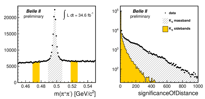
Figure 1: Left figure: invariant mass of the $K^{0}_{\scriptscriptstyle S}$ candidates, and definition of the massband (hatched region) and sidebands (colored region). Right: distribution of the significance of distance for the $K^{0}_{\scriptscriptstyle S}$ massband (data points and hatched histogram) overlaid with the distribution taken from the sidebands (colored histogram).

To reduce the dominant backgrounds arising from random combinations of particles in continuum events, we consider the ratio of the second to zeroth Fox-Wolfram moments ($R_{2}$) Fox and Wolfram (1978) and the cosine of the angle between the thrust axis of the signal $B$ candidate and that of the rest of the event (cosTBTO). We require $R_{2}<0.5$ and cosTBTO $<0.95$. These cuts are quite loose, to keep the signal reconstruction efficiency as high as reasonably possible. We then combine 30 variables sensitive to the event shape and train a multivariate BDT discriminator to distinguish between signal events (which are typically spherical) and continuum events (more jet-like). The discriminator is optimized for each individual final state, and it is utilized as one of the input variables in the final maximum likelihood fit.

As in most analyses in which the signal $B$ candidate is fully reconstructed, we use the standard beam-constrained mass $M_{\rm bc}$ and the difference between the reconstructed and expected $B$ candidate energies $\Delta E$:

$$M_{\rm bc} = \sqrt{E^{*2}_{\rm beam}c^{4}-p^{*2}_{B}c^{2}}\;,$$ (1)

$$\Delta E = E^{*}_{B}-E^{*}_{\rm beam}\;,$$ (2)

where $(E^{*}_{B},p^{*}_{B})$ are the measured energy and momentum of the candidate $B$, and $E^{*}_{\rm beam}=\sqrt{s}/2$. All quantities are calculated in the CM system. For the final fit, we require that candidates satisfy $M_{\rm bc}>5.25$ ${\mathrm{\,Ge\kern-1.00006ptV\!/}c^{2}}$ and $|\Delta E|<0.2$ $\mathrm{\,Ge\kern-1.00006ptV}$.

For $B\rightarrow V_{1}V_{2}$ decays, where $V_{i}$ is a vector meson decaying to two pseudoscalar mesons, the angular distribution, after integrating over the angle between the decay planes of $V_{1}$ and $V_{2}$, is described by:

$$\frac{1}{\Gamma}\frac{d^{2}\Gamma}{d\cos\theta_{1}d\cos\theta_{2}}=\frac{9}{4}\left[\frac{1}{4}(1-f_{L})\sin^{2}\theta_{1}\sin^{2}\theta_{2}+f_{L}\cos^{2}\theta_{1}\cos^{2}\theta_{2}\right]\;,$$ (3)

where the subscript $L$ refers to the longitudinally polarized component, and $f_{L}$ is the fraction of the longitudinally polarized component.

For the $\phi$ and $K^{*}$ resonances, the helicity angles $\theta_{H,\phi}$ and $\theta_{H,K^{*}}$ are defined as the angle between the momentum of the daughter kaon (the negatively charged in the case of the $\phi$, the only kaon in the case of the $K^{*}$) and the flight direction of the $\phi$/$K^{*}$, as measured in the $\phi$/$K^{*}$ rest frame.

The helicity angles $\theta_{H,\phi}$ and $\theta_{H,K^{*}}$ are the key variables for the measurement of the longitudinal polarization fraction $f_{L}$. In the case of $B\rightarrow\phi K$, where the spin of the $\phi$ is forced by angular momentum conservation to be perpendicular to the $\phi$ momentum, the variable $\theta_{H,\phi}$ provides additional discrimination against the continuum background and the nonresonant $B\rightarrow K^{+}K^{-}K$ component; for both backgrounds, the $\cos\theta_{H,\phi}$ distribution is expected to be roughly flat.

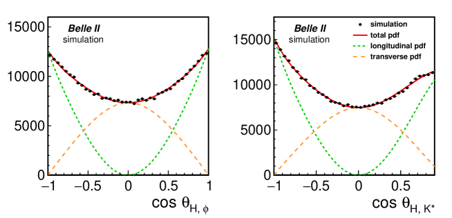
Figure 2: Distributions of $\cos\theta_{H,\phi}$ (left) and $\cos\theta_{H,K^{*}}$ (right) taken from the simulation, generated with the $f_{L}=0.5$ hypothesis and no background. The green dashed (orange long dashed) lines show the pdf’s of the longitudinal (transverse) components, while the red solid lines is the sum of the two. The distortion due to acceptance effects on the right side of the $\cos\theta_{H,K^{*}}$ distribution is clearly visible.

The distributions of $\cos\theta_{H,\phi}$ and (in a higher measure) $\cos\theta_{H,K^{*}}$ are distorted from the ideal theoretical probability density functions (pdf’s) by effects related to the non-uniform acceptance of the detector and other selection criteria. The events with $\cos\theta_{H,K^{*}}>0.9$ are particularly affected by these kinds of effects and are therefore discarded for the final fit. Figure 2 shows the expected distributions for these variables, for correctly reconstructed signal events for the hypothesis $f_{L}=0.5$.

For each decay mode, we accept at most one signal candidate per event. If an event contains more than one candidate (which happens very rarely for $B\rightarrow\phi K$ and $\sim 10\%$ of the times for $B\rightarrow\phi K^{*}$), we retain the candidate with highest vertex probability for the signal $B$ candidate. We verify in the simulation that this choice significantly improves the purity of the sample.

IV Maximum likelihood fit

The extraction of the quantities of interest is performed using an unbinned multivariate maximum likelihood (ML) fit. For the $i^{th}$ input event, the likelihood $\mathcal{L}_{i}$ is defined as:

$$\mathcal{L}_{i}=\sum_{j=1}^{m}n_{j}\mathcal{P}_{j}(\mbox{{x}}_{i})\;,$$ (4)

where $\mathcal{P}_{j}$ is the probability for the hypothesis (component) $j$ evaluated for the input variables x_i, and $n_{j}$ is the number of events in the whole sample for the component $j$ ($m$ being the total number of components considered in the fit). The probability $\mathcal{P}_{j}$ is the product of the one-dimensional probability density functions for each of the observables (input variables). One of the main assumptions of the analysis is that the correlations among these variables are negligible.

For $N$ input events, the overall likelihood $\mathcal{L}$ is:

$$\mathcal{L}=\frac{e^{-(\sum n_{j})}}{N!}\prod_{i=1}^{N}\mathcal{L}_{i}\;,$$ (5)

where the first term takes into account the Poisson fluctuations in the total number of events.

The input variables entering the ML fit are:

1. $M_{\rm bc}$;

2. $\Delta E$;

3. $C_{\rm out}^{\prime}$ (the transformed output of the continuum suppression multivariate discriminator $C_{\rm out}$);

4. $m(K^{+}K^{-})$ (invariant mass of the $\phi$ candidate);

5. $\cos\theta_{H,\phi}$ (cosine of the helicity angle of the $\phi$ candidate);

6. $m(K^{+}\pi)$ (invariant mass of the $K^{*}$ candidate);

7. $\cos\theta_{H,K^{*}}$ (cosine of the helicity angle of the $K^{*}$ candidate).

The last two variables are relevant only for the $B\rightarrow\phi K^{*}$ modes.

The components considered in the fit are:

• correctly reconstructed signal events. For the $B\rightarrow\phi K^{*}$ analysis, we float separately the yields of the longitudinal ($N_{L}$) and transverse ($N_{T}$) components, and compute $f_{L}$ taking into account the different reconstruction efficiencies $\varepsilon_{L}$ and $\varepsilon_{T}$ for the longitudinally and transversely polarized events, respectively:

  $$f_{L}=\frac{N_{L}/\varepsilon_{L}}{N_{L}/\varepsilon_{L}+N_{T}/\varepsilon_{T}}\,.$$ (6)

  The yield parameters are allowed to take negative values (thus the result on $f_{L}$ may be outside the physical $[0,1]$ range);

• self-crossfeed (SXF). This component is constituted of signal events in which one or more candidate particles originate from the unreconstructed $B$. For the $B\rightarrow\phi K$ analyses, the fraction of self-crossfeed events is negligible, so this component is not considered;

• nonresonant, given by $B\rightarrow K^{+}K^{-}K^{(*)}$ events. Early BaBar Lees et al. (2012) and Belle Nakahama et al. (2010) analyses have shown that this component accounts for $\mathcal{(}10\%)$ of the events observed in the $\phi$ mass region; this justifies a separate treatment for this category of events;

• other $B\kern 1.79993pt\overline{\kern-1.79993ptB}{}$ backgrounds;

• continuum background, by far the dominant source of background for this analysis.

The continuum background is modeled from the data, excluding the signal box defined by the requirements $M_{\rm bc}>5.27$ ${\mathrm{\,Ge\kern-1.00006ptV\!/}c^{2}}$ and $|\Delta E|<0.1$ $\mathrm{\,Ge\kern-1.00006ptV}$. The pdf’s of all the other components are determined from the simulation (Agostinelli et al. (2003), Lange (2001)).

In the nominal fit, we allow the yields of the signal component(s) and of the continuum background, to vary, along with the following parameters describing the shape of the continuum background: the slope of the Argus function Albrecht et al. (1990) that is used to fit the $M_{\rm bc}$ distribution; the slopes of the (non peaking) $\Delta E$, $m(K^{+}K^{-})$, and $m(K^{+}\pi)$ components; the fractions of the peaking components in the $m(K^{+}K^{-})$ and $m(K^{+}\pi)$ distributions; and the mean of the core Gaussian component of the $C_{\rm out}^{\prime}$ variable.

The shapes and normalization of the SXF, nonresonant, and other $B\kern 1.79993pt\overline{\kern-1.79993ptB}{}$ background components are fixed to the expectations from the simulation. The yield of the nonresonant component is fixed to 10% of the (total) signal yield; the fraction of the SXF component relative to the correctly reconstructed signal is kept constant to the predictions of the simulation; and the yield of the other $B\kern 1.79993pt\overline{\kern-1.79993ptB}{}$ backgrounds is set to the value predicted by the generic Monte Carlo. All these quantities are varied separately by $\pm 50\%$ for the determination of the systematic uncertainties.

The fitting procedure has been tested extensively using toy Monte Carlo experiments that preserve the correlations (if any) among the input variables and thus test the main assumption of the fit model, which assumes all correlations to be negligible. No significant bias has been detected.

The events in the signal box have not been analyzed until the fit procedure was clearly defined, and full confidence was reached from studies on the simulation and data sidebands.

V Results

Tables 1 and 2 summarize the results of the ML fit applied to the Summer 2020 Belle II dataset. In all cases, we see a significant signal, whose significance (taking only into account the statistical uncertainties) ranges from 6.4 to 11.5 standard deviations. The longitudinal polarization fraction in the $B\rightarrow\phi K^{*}$ modes $f_{L}$ is very consistent with the expectations. The branching ratios have been computed using the formula:

$$\mathcal{B}(B\rightarrow X)=\frac{N_{sig}}{N(B\kern 1.79993pt\overline{\kern-1.79993ptB}{})\times 2\times\varepsilon\times{\rm ProdBF}}\,,$$ (7)

where $N_{sig}$ is the number of fitted signal events, $N(B\kern 1.79993pt\overline{\kern-1.79993ptB}{})$ is the number of (charged or neutral) $B\kern 1.79993pt\overline{\kern-1.79993ptB}{}$ pairs, $\varepsilon$ is the signal reconstruction efficiency, and ProdBF is the product of the branching fractions of all the intermediate resonances involved. For the $B\rightarrow\phi K^{*}$ modes, the branching ratio is the sum of the partial branching ratios for the longitudinal and transverse components, which have different reconstruction efficiencies.

Table 1: Summary of the fit results of the $B\rightarrow\phi K$ modes. The upper part shows the information about the yields (with statistical uncertainty only) of the signal (nSig), SXF (nSXF), nonresonant (nNR), and other $B\kern 1.79993pt\overline{\kern-1.79993ptB}{}$ backgrounds (nBBbar) components. The bottom part displays the reconstruction efficiencies and the measured branching fractions.

	$B^{+}\rightarrow\phi K^{+}$	$B^{0}\rightarrow\phi K^{0}_{\scriptscriptstyle S}$
Events in fit	1576	695
nSig	$55.0\pm 8.9$	$15.7\pm 4.9$
nSXF	0.0 (fixed)	0.0 (fixed)
nNR	5.4 (fixed)	1.6 (fixed)
nBBbar	13.0 (fixed)	3.4 (fixed)
Significance (stat. only)	11.5$\sigma$	6.4$\sigma$
$\varepsilon$ (%)	$42.5\pm 3.0$	$41.9\pm 4.8$
$\mathcal{B}(\times 10^{-6})$	$6.7\pm 1.1\pm 0.5$	$3.0\pm 0.9\pm 0.4$

Table 2: Summary of the fit results of the $B\rightarrow\phi K^{*}$ modes. The upper part shows the information about the yields (with statistical uncertainty only) of the longitudinally polarized signal (nSigL), transversely polarized signal (nSigT), SXF (nSXF), nonresonant (nNR), and other $B\kern 1.79993pt\overline{\kern-1.79993ptB}{}$ backgrounds (nBBbar) components. The bottom part displays the reconstruction efficiencies, the measured branching fractions, and longitudinal polarization fractions $f_{L}$.

	$B^{+}\rightarrow\phi K^{*+}$	$B^{0}\rightarrow\phi K^{*0}$
Events in fit	2133	3055
nSigL	$17.6\pm 5.7$	$25.0\pm 7.0$
nSigT	$15.2\pm 5.5$	$22.7\pm 7.1$
nSXF	3.7 (fixed)	4.8 (fixed)
nNR	3.3 (fixed)	4.7 (fixed)
nBBbar	22.6 (fixed)	38.2 (fixed)
Significance (stat. only)	$6.4\sigma$	$9.8\sigma$
$\varepsilon_{L}$ (%)	$31.4\pm 2.5$	$32.7\pm 1.9$
$\varepsilon_{T}$ (%)	$36.8\pm 2.9$	$38.6\pm 2.3$
$\mathcal{B}(\times 10^{-6})$	$21.7\pm 4.6\pm 1.9$	$11.0\pm 2.1\pm 1.1$
$f_{L}$	$0.58\pm 0.23\pm 0.02$	$0.57\pm 0.20\pm 0.04$

In general, the results are in good agreement with the world averages Tanabashi et al. (2018). The observed branching fraction of $B\rightarrow\phi K^{*}$ is approximately two standard deviations higher than the average of the previous results. We checked the stability of the fit by discarding in turn one of the input variables: in all cases the variations of the signal yield are less than two events, much smaller than the statistical uncertainty. We also perform a test in which we remove both helicity angles (so that we lose sensitivity to the polarization), and again the fitted yield is quite compatible with the nominal fit. We conclude that the fit is stable, and the higher than expected branching ratio is probably due to a statistical fluctuation.

Figures 3–6 show the projection plots of the fit variables utilized for each channel. In order to enhance the signal component, a cut on the likelihood ratio (for signal over all the hypotheses, with the likelihood being computed using all the variables with the exception of the one plotted) at 0.5 has been applied.

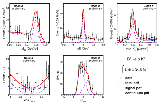
Figure 3: Signal enhanced projection plots for the fit variables of $B^{+}\rightarrow\phi K^{+}$. The solid red curve represents the total fit function, the magenta dashed line shows the signal component, and the blue dotted line corresponds to the continuum background.

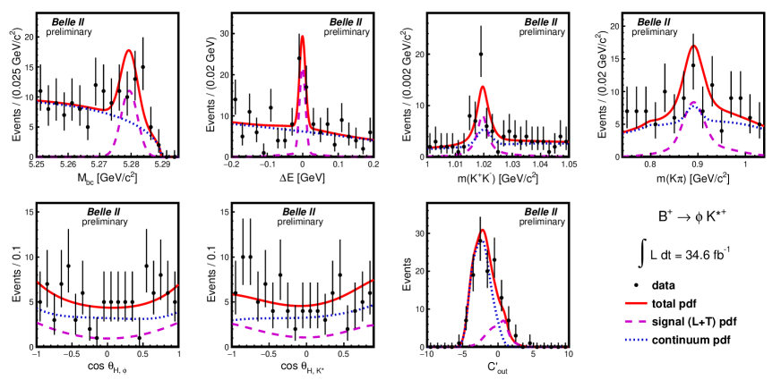
Figure 4: Signal enhanced projection plots for the fit variables of $B^{+}\rightarrow\phi K^{*+}$. The solid red curve represents the total fit function, the magenta dashed line shows the signal component, and the blue dotted line corresponds to the continuum background.

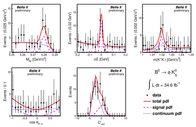
Figure 5: Signal enhanced projection plots for the fit variables of $B^{0}\rightarrow\phi K^{0}_{\scriptscriptstyle S}$. The solid red curve represents the total fit function, the magenta dashed line shows the signal component, and the blue dotted line corresponds to the continuum background.

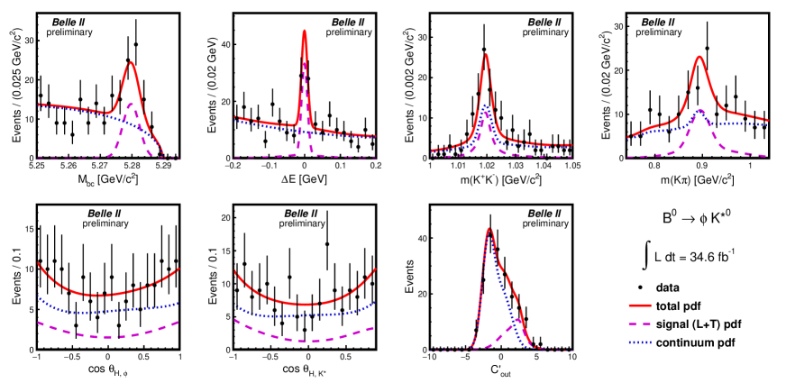
Figure 6: Signal enhanced projection plots for the fit variables of $B^{0}\rightarrow\phi K^{*0}$. The solid red curve represents the total fit function, the magenta dashed line shows the signal component, and the blue dotted line corresponds to the continuum background.

Finally, we evaluate the compatibility of our results for $f_{L}$ with the extreme hypotheses $f_{L}=0$ and $f_{L}=1$. To do this, we respectively fix to 0 the yield of the longitudinal and transverse component, and compute $\sqrt{-2(\log\mathcal{L}-\log\mathcal{L}_{0})}$, where $\mathcal{L}$ is the value of the likelihood computed for the tested hypothesis, and $\mathcal{L}_{0}$ is the likelihood of the nominal fit. The lowest significance ($\sim 4.6\sigma$) is observed for $f_{L}=1$ in the $B^{+}\rightarrow\phi K^{*+}$ channel; in all other cases, the significance exceeds $5\sigma$.

VI Systematics

Tables 3 and 4 summarize the systematic uncertainties affecting the measurements of the branching ratios and of $f_{L}$, respectively.

Table 3: Summary of the systematic uncertainties, in per cent, affecting the signal yields. The uncertainties are categorized as multiplicative (M) or additive (A).

Source	$B^{+}\rightarrow\phi K^{+}$	$B^{+}\rightarrow\phi K^{*+}$	$B^{0}\rightarrow\phi K^{0}_{\scriptscriptstyle S}$	$B^{0}\rightarrow\phi K^{*0}$
Tracking efficiency (M)	2.7	4.6	3.6	3.6
$K^{0}_{\scriptscriptstyle S}$ reconstruction efficiency (M)	–	6.3	10.8	–
Kaon ID efficiency (M)	6.4	1.1	1.0	4.7
Number of $B\kern 1.79993pt\overline{\kern-1.79993ptB}{}$ events (M)	2.7	2.7	2.7	2.7
Modeling of $C_{\rm out^{\prime}}$ (A)	1.3	1.2	1.0	5.9
$B\kern 1.79993pt\overline{\kern-1.79993ptB}{}$ background yield (A)	0.3	1.2	1.4	2.3
Nonresonant yield (A)	3.1	1.8	4.5	3.2
SXF fraction (A)	–	0.6	–	1.0
Total multiplicative	7.5	8.3	11.7	6.5
Total additive	3.4	2.5	4.8	7.1
Total	8.2	8.7	12.7	9.7

Table 4: Summary of the systematic uncertainties (expressed in absolute values) affecting the measurement of $f_{L}$ in the $B\rightarrow\phi K^{*}$ modes.

Source	$B^{+}\rightarrow\phi K^{*+}$	$B^{0}\rightarrow\phi K^{*0}$
Acceptance function	0.014	0.007
Modeling of $C_{\rm out^{\prime}}$	0.001	0.035
$B\kern 1.79993pt\overline{\kern-1.79993ptB}{}$ background yield	0.002	0.009
Nonresonant yield	0.006	0.008
SXF fraction	0.001	0.003
Total	0.015	0.038

We consider the following sources of systematics:

• tracking efficiency: we (linearly) add 0.91% for each charged track in the signal final state;

• $K^{0}_{\scriptscriptstyle S}$ reconstruction efficiency: we use a data control sample, and we observe that the $K^{0}_{\scriptscriptstyle S}$ reconstruction efficiency decreases (compared to the simulation) linearly with the flight length. We apply an uncertainty of 1% for each cm of average flight length of the $K^{0}_{\scriptscriptstyle S}$ candidate;

• charged kaon identification: we take the difference between the reconstruction efficiency for signal candidates measured using only Monte Carlo information and the efficiency obtained by shifting the kaon identification efficiency to what is measured on a data sample of $D^{*+}\rightarrow\pi^{+}D^{0}(\rightarrow K^{-}\pi^{+})$. This uncertainty is larger for the $\phi K^{+}$ and $\phi K^{*0}$ mode, as the charged kaon typically has a much higher momentum than the kaons produced by the $\phi$ decay, and the agreement between data and simulation is currently much better at lower momenta;

• number of $B\kern 1.79993pt\overline{\kern-1.79993ptB}{}$ events: we assign a 2.7% systematic error, which includes the uncertainty on cross-section, integrated luminosity, and potential shifts from the peak CM energy during the run periods;

• modeling of the $C_{\rm out^{\prime}}$ variable: we take the difference in the results obtained when the shape of the $C_{\rm out^{\prime}}$ is determined from the data sidebands (nominal fit) and when the shape is modeled from the simulation;

• yields of SXF, nonresonant, and $B\kern 1.79993pt\overline{\kern-1.79993ptB}{}$ background components: we individually vary by $\pm 50\%$ the yield of each component, and take the difference of the results (with respect to the nominal fit) as systematic uncertainty;

• acceptance function for the helicity angles (relevant only for the measurement of $f_{L}$). The pdf’s of $\cos\theta_{H,\phi}$ and $\cos\theta_{H,K^{*}}$ are the products of a theoretical pdf’s and an acceptance function. We evaluate the systematic uncertainty by taking the difference between the nominal fit results and the cases in which the deviations from unity of the acceptance function are doubled or removed (uniform acceptance).

VII Conclusions

In conclusion, we have observed all four $B\rightarrow\phi K^{(*)}$ channels in the Summer 2020 Belle II dataset of 34.6$\mbox{\,fb}^{-1}$, with branching ratios that are in good or fair (for the $B^{+}\rightarrow\phi K^{*+}$ case) agreement with the world averages Tanabashi et al. (2018). The measurement of the longitudinal polarization fraction $f_{L}$ is in excellent agreement with our expectations.

The results of this analysis are summarized in Table 5. We also compute the isospin ratios

$$I_{\phi K^{(*)}}=\frac{\mathcal{B}(B^{+}\rightarrow\phi K^{(*)+})}{\mathcal{B}(B^{0}\rightarrow\phi K^{(*)0})}\,,$$ (8)

which are interesting observables for detecting signs of physics beyond the standard model (e.g. in Feldmann et al. (2008)) and that we measure to be in reasonably good agreement with unity.

Table 5: Summary of the results obtained in this analysis.

	This analysis	World Average Tanabashi et al. (2018)
$\mathcal{B}(\times 10^{-6})$
$\phi K^{+}$	$6.7\pm 1.1\pm 0.5$	$8.8\pm 0.7$
$\phi K^{0}$	$5.9\pm 1.8\pm 0.7$	$7.3\pm 0.7$
$I_{\phi K}$	$1.1\pm 0.4\pm 0.2$	$1.21\pm 0.15$
$\phi K^{*+}$	$21.7\pm 4.6\pm 1.9$	$10.0\pm 2.0$
$\phi K^{*0}$	$11.0\pm 2.1\pm 1.1$	$10.0\pm 0.5$
$I_{\phi K^{*}}$	$2.0\pm 0.6\pm 0.3$	$1.00\pm 0.21$
$f_{L}$
$\phi K^{*+}$	$0.58\pm 0.23\pm 0.02$	$0.50\pm 0.05$
$\phi K^{*0}$	$0.57\pm 0.20\pm 0.04$	$0.497\pm 0.017$

References

- Altmannshofer et al. (2019) W. Altmannshofer et al. (Belle-II), PTEP 2019, 123C01 (2019), [Erratum: PTEP 2020, 029201 (2020)], arXiv:1808.10567 [hep-ex] .
- Tanabashi et al. (2018) M. Tanabashi et al. (Particle Data Group), Phys. Rev. D98, 030001 (2018).
- Kagan (2004) A. L. Kagan, Phys. Lett. B 601, 151 (2004), arXiv:hep-ph/0405134 .
- Beneke et al. (2006) M. Beneke, J. Rohrer, and D. Yang, Phys. Rev. Lett. 96, 141801 (2006), arXiv:hep-ph/0512258 .
- (5) T. Abe et al. (Belle-II), arXiv:1011.0352 [physics.ins-det] .
- Akai et al. (2018) K. Akai, K. Furukawa, and H. Koiso (SuperKEKB), Nucl. Instrum. Meth. A907, 188 (2018), arXiv:1809.01958 [physics.acc-ph] .
- Bevan et al. (2014) A. J. Bevan et al. (BaBar, Belle), Eur. Phys. J. C74, 3026 (2014), arXiv:1406.6311 [hep-ex] .
- Aubert et al. (2005) B. Aubert et al. (BaBar), Phys. Rev. Lett. 95, 042001 (2005), arXiv:hep-ex/0504001 .
- Fox and Wolfram (1978) G. C. Fox and S. Wolfram, Phys. Rev. Lett. 41, 1581 (1978).
- Lees et al. (2012) J. Lees et al. (BaBar), Phys. Rev. D 85, 112010 (2012), arXiv:1201.5897 [hep-ex] .
- Nakahama et al. (2010) Y. Nakahama et al. (Belle), Phys. Rev. D 82, 073011 (2010), arXiv:1007.3848 [hep-ex] .
- Agostinelli et al. (2003) S. Agostinelli et al. (GEANT4), Nucl.Instrum.Meth. A506, 250 (2003).
- Lange (2001) D. J. Lange, Proceedings, 7th International Conference on B physics at hadron machines (BEAUTY 2000): Maagan, Israel, September 13-18, 2000, Nucl. Instrum. Meth. A462, 152 (2001).
- Albrecht et al. (1990) H. Albrecht et al. (ARGUS), Phys. Lett. B 241, 278 (1990).
- Feldmann et al. (2008) T. Feldmann, M. Jung, and T. Mannel, JHEP 08, 066 (2008), arXiv:0803.3729 [hep-ph] .