Entanglement enhanced and one-way steering in $\mathcal{PT}$-symmetric cavity magnomechanics

Abstract

We study creation of entanglement and quantum steering in a parity-time- ($\mathcal{PT}$ -) symmetric cavity magnomechanical system. There is magnetic dipole interaction between the cavity and photon-magnon, and there is also magnetostrictive interaction which is induced by the phonon-magnon coupling in this system. By introducing blue-detuned driving microwave field to the system, the bipartite entanglement of the system with $\mathcal{PT}$ -symmetry is significantly enhanced versus the case in the conventional cavity magnomechanical systems (loss-loss systems). Moreover, the one-way quantum steering between magnon-phonon and photon-phonon modes can be obtained in the unbroken-PT -symmetric regime. The boundary of stability is demonstrated and this show that the steady-state solutions are more stable in the gain and loss systems. This work opens up a route to explore the characteristics of quantum entanglement and steering in magnomechanical systems, which might have potential applications in quantum state engineering and quantum information.

I Introduction

In recent years, cavity magnomechanical system (CMM system) has attracted extensive attentions in the cavity quantum electrodynamics. This CMM system consists of a three dimensional rectangular microwave cavity and a single-crystal yttrium-iron-garnet (YIG) sphere inside. Owing the high spin density and the strong spin-spin exchange interactions, the Kittel mode in the YIG sphere can achieve strong Huebl et al. (2013); Zhang et al. (2014) and even ultrastrong coupling Bourhill et al. (2016) to the microwave cavity mode. And this strong coupling can be achieved even at room temperature Zhang et al. (2015a). On the other hand, the CMM systems are developed from optomechanical systems Aspelmeyer et al. (2014); Zeng et al. (2020); Xiong et al. (2020); Zhang et al. (2019); Liao et al. (2020); Zeng et al. (2019); Zhang et al. (2014) which achieve the interaction between phonons and optical or microwave photons by radiation force or electrostatic force. While the magnetostrictive force of the YIG sphere is applied to realize the coupling between phonons and magnons in the CMM systems. Comparing with the optomechanical systems, the CMM systems have the advantages of high adjustability and low loss. Therefore, it provides a good opportunity for realizing highly tunable information processing in the hybrid quantum systems Zhang et al. (2015b). J. Q. You $et$ $al$. report that the bistability of cavity magnon polaritons Wang et al. (2018a), G. S. Agarwal $et$ $al$. show that the tripartite entanglement among magnons, photons, and phonons Li et al. (2018a). Besides, the high-order sideband generationLiu et al. (2018), magnon Kerr effectWang et al. (2016), the light transmission in cavity-magnon system Wang et al. (2018b) and others are also studied Woods (2001); Gao et al. (2017); Wang et al. (2020); Yuan et al. (2020); Huai et al. (2019); Ding and Li (2019a, b); Zhao et al. (2020); Gao et al. (2019).

The developments in Parity-time-symmetry ($\mathcal{PT}$-symmetry) optical structure resulted in the birth of the new field which attracted considerable interest Chong et al. (2011); Bender and Boettcher (1998); Jing et al. (2014). In the past, people believed that only Hermitian Hermitonian has real eigenvalue spectra, while C. M. Bender $et$ $al$. have proved that the $\mathcal{PT}$-symmetric non-Hermitian Hamiltonian ($[H,PT]=0$) can also has real eigenvalue spectra Bender and Boettcher (1998). Up to present, $\mathcal{PT}$-symmetry been widely applied to quantum optics, quantum information processing, and propagation, including the optical non-reciprocity in $\mathcal{PT}$-symmetric whispering-gallery microcavities (WGM) Peng et al. (2014), the detection sensitivity of weak mechanical motion Liu et al. (2016), realizing quantum chaos Lü et al. (2015), strengthening optics nonlinearityLi et al. (2015a), nonreciprocal light propagation Liu et al. (2017) and so on Li et al. (2017); Makris et al. (2008); Tchodimou et al. (2017); El-Ganainy et al. (2018); Xu et al. (2020). In addition, it is difficult to achieve ideal $\mathcal{PT}$-symmetry under the strict requirements of balanced gain and loss. Here, we study the non-equilibrium effective $\mathcal{PT}$-symmetric system, which works in microwave regime.

In this work, we propose to construct a $\mathcal{PT}$-symmetric CMM system with the active cavity and passive magnon modes. The magnetostrictive (radiation pressure like) interaction mediates the coupling between magnons and phonons. And the cavity photons and magnons are coupled via magnetic dipole interaction. We show the stability parameter boundary of the system which is driven by a blue-detuned microwave field. Here, $\mathcal{PT}$-symmetry leads to a strong bipartite entanglement among the mechanical mode, the optical field inside the gain cavity and magnon mode, the logarithmic negativity is used to measure the continuous variable (CV) entanglement Adesso et al. (2004). And the potential feasibility of the experiment is discussed. G. S. Agarwal $et$ $al$. first studied the entanglement in CMM system Li et al. (2018a), our work is based on it and consider the enhancement effect of $\mathcal{PT}$-symmetry on the entanglement. Furthermore, we show that the $\mathcal{PT}$-symmetry can induce one-way quantum steering between magnon-phonon and photon-phonon modes. As we know, the quantum steering is intrinsically different from quantum entanglement and Bell nonlocality for its asymmetric characteristics and it has potential applications in the quantum information protocols, such as device-independent quantum key distribution.

The structure of the paper is as follows. In Sec. II, we introduce the Hamiltonian and dynamical equations of the whole systems. In Sec. III, the stability of the system is discussed. In Sec. IV, we show that by introducing $\mathcal{PT}$-symmetry, the entanglement is obviously enhanced and one-way steering can be obtained. Finally, a concluding summary is given.

II Model and
dynamical Hamiltonian

We utilize a $\mathcal{PT}$-symmetric CMM system as shown in Fig. 1(a), which consists of microwave cavity photons (gain) and magnons (loss). The magnons in the YIG sphere are collective excitation of magnetization, and the uniform magnon mode is driven by an adjustable microwave field. Furthermore, the magnetic dipole interaction leads to the coupling between magnon mode and active cavity mode.

Owing to the magnetostrictive effect, the YIG sphere can be considered as an excellent mechanical resonator Zhang et al. (2015b). Therefore, the term of coupling between magnons and phonons can be introduced into Hamiltonian of the system. And the magnetostrictive coupling strength is determined by the mode overlap between the magnon and phonon modes. In general, the magnomechanical coupling is very weak Zhang et al. (2015b). However, it can be effectively enhanced by a microwave driving field Wang et al. (2018a); Li et al. (2018a).

The equivalent mode-coupling model is given in Fig. 1(b). The size of the YIG sphere we considered is much smaller than the wavelength of the microwave field. Hence, the interaction between microwave cavity photons and phonons induced by the radiation pressure is neglected. In a rotating-wave approximation, the Hamiltonian of the whole system is given by ($\hbar=1$) Li et al. (2018a)

$$H = \omega_{a}a^{\dagger}a+\omega_{m}m^{\dagger}m+g_{ma}(a^{\dagger}m+m^{\dagger}a)$$

$$+\frac{\omega_{b}}{2}(x^{2}+p^{2})+g_{mb}m^{\dagger}mx$$

$$+i\varepsilon_{d}(m^{\dagger}e^{-i\omega_{d}t}-me^{i\omega_{d}t}),$$

where $a(a^{\dagger})$ and $m(m^{\dagger})$ are the annihilation(creation) operators of the cavity mode and the uniform magnon mode at the frequency $\omega_{a}$ and $\omega_{m}$, respectively ($[O,O^{\dagger}]=1,O=a,m$). The magnon frequency $\omega_{m}$ can be easily adjusted by altering the external bias magnetic field $H$ via $\omega_{m}=\gamma_{g}H$, where $\gamma_{g}$ is the gyromagnetic ratio ($\gamma/2\pi=28GHz/T$). $x$ and $p$ are the dimensionless position and momentum quadrature of the mechanical mode with the frequency $\omega_{b}$ ($[x,p]=1$). The coupling rate of the magnon-cavity interaction is $g_{ma}$ and $\omega_{d}$ is frequency of driven field. Here, the Hamiltonian in Eq.(II) does not include the gain.

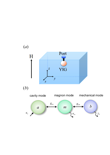
Figure 1: (a) Schematic illustration of the system, a YIG sphere is placed in a three-dimensional cavity, and it is connected with the inner wall of the cavity by a silicon fiber. The port is for driving the YIG sphere via a microwave field. A bias magnetic field $H$ along the $z$-axis is used to realize magnon-photon coupling by magnetic dipole interaction. It is worth mentioning that the directions of the bias magnetic field, the drive field, and the magnetic field of the cavity mode are perpendicular to each other. (b) The equivalent mode-coupling model.

Under the assumption of the low-lying excitations, the Rabi frequency $\varepsilon_{d}$ is $\frac{\sqrt{5}}{4}\gamma_{g}\sqrt{N_{t}}B_{0}$, and it denotes the coupling strength between the magnon mode and the driving field with the amplitude $B_{0}$. The total number of the spins $N_{t}$ is given by $\rho V$, where the spin density $\rho=$ $4.22\times 10^{27}$m^-3, and $V$ is the volume of the YIG sphere.

After a rotating frame at the frequency $\omega_{d}$ of the above Hamiltonian, one derives the following set of the Heisenberg-Langevin equations:

$$\dot{a} = (-i\Delta_{a}+\kappa_{a})a-ig_{ma}m+\sqrt{2\kappa_{a}}a^{in},$$

$$\dot{m} = (-i\Delta_{m}-\kappa_{m})m-ig_{ma}a-ig_{mb}mx+\varepsilon_{d}+\sqrt{2\kappa_{m}}m^{in},$$

$$\dot{x} = \omega_{b}p,$$ (2)

$$\dot{p} = -\omega_{b}x-\gamma_{b}p-g_{mb}m^{\dagger}m+\xi,$$

where the detuning $\Delta_{a(m)}=\omega_{a(m)}-\omega_{d}$, $\kappa_{a}$ is the gain rate of the cavity mode, $\kappa_{m}$ and $\gamma_{b}$ are the dissipation rates of magnon and mechanical modes, respectively. $a^{in},m^{in}$ and $\xi$ are input noise operators of cavity, magnon and mechanical modes. With a Markovian approximation, the input noise correlation functions are shown as: $\left\langle a^{in}(t)a^{in\dagger}(t^{\prime})\right\rangle=(n_{a}+1)\delta(t-t^{\prime})$, $\left\langle a^{in\dagger}(t)a^{in}(t^{\prime})\right\rangle=n_{a}\delta(t-t^{\prime})$, $\left\langle m^{in}(t)m^{in\dagger}(t^{\prime})\right\rangle=(n_{m}+1)\delta(t-t^{\prime})$, $\left\langle m^{in\dagger}(t)m^{in}(t^{\prime})\right\rangle=n_{m}\delta(t-t^{\prime})$, $\left\langle\xi(t)\xi^{\dagger}(t^{\prime})\right\rangle=(n_{b}+1)\delta(t-t^{\prime})$ and $\left\langle\xi^{\dagger}(t)\xi(t^{\prime})\right\rangle=n_{b}\delta(t-t^{\prime})$. Here, $n_{\mu}=(e^{\hbar\omega_{\mu}/k_{B}T}-1)$($\mu=a,m,b$) with $k_{B}$ the Boltzmann constant and $T$ the environmental temperature, and these $n_{\mu}$ are equilibrium mean thermal photon, magnon, and phonon numbers, respectively.

In order to better understand the broken $\mathcal{PT}$-symmetry regimes and the unbroken $\mathcal{PT}$-symmetry regimes of this system, we only focus on the cavity and magnon modes. And the driving field in Eq.(II) can be neglected as the same reason in Peng et al. (2014). By the $\mathcal{PT}$ operation, the Hamiltonian can be described by a second-order matrix, i.e.,

$$H_{\mathcal{PT}}=\mathcal{PT}H\mathcal{PT}=(\hat{a}^{\dagger}\text{ }\hat{m}^{\dagger})\left(\begin{array}[]{cc}\Delta_{m}+i\kappa_{m}&g_{ma}\\ g_{ma}&\Delta_{a}-i\kappa_{a}\end{array}\right)(\hat{a}\text{ }\hat{m})^{T},$$ (3)

where the parity operation $\mathcal{P}$ acting on the Hamiltonian can interchange the loss and gain of the cavity and magnon modes, i.e., $\hat{a}\Longleftrightarrow-\hat{m}$ and $\hat{a}^{\dagger}\Longleftrightarrow-\hat{m}^{\dagger}.$And the time reversal operation $\mathcal{T}$ on $H$ can reverse the sign of complex number $i$. After setting $\Delta_{a}=\Delta_{m}=\Delta$, the eigenfrequencies of the Hamiltonian in Eq.(3) can be written as

$$\omega_{\pm}=-\Delta-i(\kappa_{m}-\kappa_{a})/2\pm\sqrt{g_{ma}^{2}-(\kappa_{a}+\kappa_{m})^{2}/4}.$$ (4)

In order to make the Hamiltonian be $\mathcal{PT}$-symmetry, the eigenfrequencies should be real. According to Eq.(4), with the the condition: $\Delta_{a}=\Delta_{m}=\Delta$, $2g_{ma}>\kappa_{a}+\kappa_{m}$ and $\kappa_{m}=\kappa_{a}$, we have $H^{\mathcal{PT}}=H$ and $[H,\mathcal{PT]}=0$, that is to say, this Hamiltonian is strictly in unbroken $\mathcal{PT}$-symmetry regime. Correspondingly, the broken-$\mathcal{PT}$-symmetry regime holds for the case of $2g_{ma}<\kappa_{a}+\kappa_{m}$. In addition, the phase transition between the broken-$\mathcal{PT}$-symmetry and unbroken $\mathcal{PT}$-symmetry regimes, i.e., $2g_{ma}=\kappa_{a}+\kappa_{m}$ is exceptional point (EP).

It is worth noting that under the condition of non-equilibrium ($\kappa_{m}\neq\kappa_{a}$), even if the eigenvalues of the system are complex, the system still has phase transition, and phase transformation point remains unchanged. Actually, choosing appropriate reference frame, the non-equilibrium system is an effective $\mathcal{PT}$-symmetric system. Physically, this system can be considered as a strict $\mathcal{PT}$-symmetric system coupled to an effective reservoir with decay rate $\kappa_{m}-\kappa_{a}$. A lot of work have adopted the effective $\mathcal{PT}$-symmetric systemsChong et al. (2011); Zhang et al. (2017); Huai et al. (2019).

Next, the values of the specific parameters used in this work are given and they are easy to be achieved in experiments Zhang et al. (2015b); Wang et al. (2018a). In our discussion, $\omega_{a}/2\pi=\omega_{m}/2\pi=10.1GHz$, $\omega_{b}/2\pi=10MHz$, $\gamma_{b}/2\pi=10Hz$, $g_{mb}/2\pi=0.2Hz,\kappa_{m}=1MHz$, and the temperature is $20$mK.

III STABILITY OF SYSTEM

In this section, in order to quantify the entanglement of this system, an important condition is the existence of asymptotic steady state and system will keep the state for a long evolution time. Hence, we discuss the stability of the steady-state solutions.

Because the magnon mode is directly driven by a strong microwave source, it leads to a large number of magnons $\left|\left\langle m\right\rangle\right|\gg 1$ at the steady state. And according to the cavity-magnon beam splitter interaction in Eq.(4), the cavity field has a large amplitude $\left|\left\langle a\right\rangle\right|\gg 1$. Therefore, each Heisenberg operator can rewritten as a sum of its steady-state mean value and its corresponding quantum fluctuation, i.e., $O(t)=O_{s}+\delta O(t)$ $(O=a,m,x,p)$. Then we study the stability of the system through a linear stability analysis Lathrop (2015). From the Heisenberg-Langevin equations in Eq.(2), the dynamical equation of the quantum fluctuation is written by a compact equation, i.e.,

$$\dot{\nu}(t)=M\nu(t)+r(t),$$ (5)

where $v(t)$ is the vector of the quantum fluctuations, and $r(t)$ is the noise vector. They can be expressed as $v(t)=[\delta a(t)$, $\delta a^{\dagger}(t)$, $\delta m(t)$, $\delta m^{\dagger}(t)$, $\delta x(t)$, $\delta p(t)]^{T}$ and $r(t)=[\sqrt{2\kappa_{a}}\delta a^{in}(t)$, $\sqrt{2\kappa_{a}}\delta a^{in\dagger}(t)$, $\sqrt{2\kappa_{m}}\delta m^{in}(t)$, $\sqrt{2\kappa_{m}}\delta m^{in\dagger}(t)$, $0$, $\xi(t)]^{T}$, respectively. The matrix $M$ is the coefficient matrix of the system, which reflects the stability or stochastic property of the system. Here, $M$ can be obtained as

$$\left(\begin{array}[]{cccccc}-i\Delta_{a}+\kappa_{a}&0&-ig_{ma}&0&0&0\\ 0&i\Delta_{a}+\kappa_{a}&0&ig_{ma}&0&0\\ -ig_{ma}&0&-i\tilde{\Delta}_{m}-\kappa_{m}&0&-iG&0\\ 0&ig_{ma}&0&i\tilde{\Delta}_{m}-\kappa_{m}&iG&0\\ 0&0&0&0&0&\omega_{b}\\ 0&0&-G&-G&-\omega_{b}&-\gamma_{b}\end{array}\right),$$ (6)

where $G=g_{mb}\left|m_{s}\right|$ is the coherent-driving-enhanced magnomechanical coupling strength, $m_{s}$ can be obtained by solving the steady-state mean value of Eq.(2), i.e.,

$$m_{s}=\frac{\varepsilon_{d}(i\Delta_{a}-\kappa_{a})}{g_{ma}^{2}+(i\Delta_{a}-\kappa_{a})(i\tilde{\Delta}_{m}+\kappa_{m})},$$ (7)

where $\tilde{\Delta}_{m}=\Delta_{m}+g_{mb}\left|q_{s}\right|$ is the effective magnon-drive detuning.

The stability analysis of the system can be done according to the eigenvalues of the matrix $M$, it can be seen that the matrix $M$ has three pairs of conjugate eigenvalues. And the real parts of the eigenvalues are known as the Lyapunov exponents Benettin et al. (1980), if the maximal Lyapunov exponent is negative, the system is stable. Contrarily, the maximal Lyapunov exponent is positive indicates the system is unstable Lü et al. (2015); Li et al. (2015b).

In Figs.2 (a), (b) and (c), the boundary of linear stability is shown. The light area indicates that the maximal Lyapunov exponent is negative, in other words, the system is stable. The remaining dark area indicates that the system is unstable. Here, we use $\kappa_{a}>0$ and $\kappa_{a}<0$ to represent the active-passive CMM system and the conventional CMM system, respectively. Comparison of Figs.2(a) and 2(b), the stable area of (b) $\kappa_{a}=0.2\kappa_{m}$ is obviously larger than that of (a) $\kappa_{a}=-0.2\kappa_{m}$. It means that the stability of active-passive CMM system ($\kappa_{a}>0$) is better than that of the conventional CMM system ($\kappa_{a}<0$) within the range of parameters we considered. Then from Fig.2(c), it can be conclude that the stability of the active-passive CMM system decreases with the system approaches the gain-loss balance. Finally, it can be seen that the stability can be improved by the increase of $g_{ma}$ in the active-passive CMM system in Fig.2(d).

When the active-passive CMM system is in the EP or broken $\mathcal{PT}$-symmetry regime, in order to get a stable system, $G$ needs to be small enough compared to $g_{ma}$, which leads to a very weak entanglement (it will be discussed in detail in the next section). As a consequence, we only focus on the stability of unbroken $\mathcal{PT}$-symmetry regime in this section.

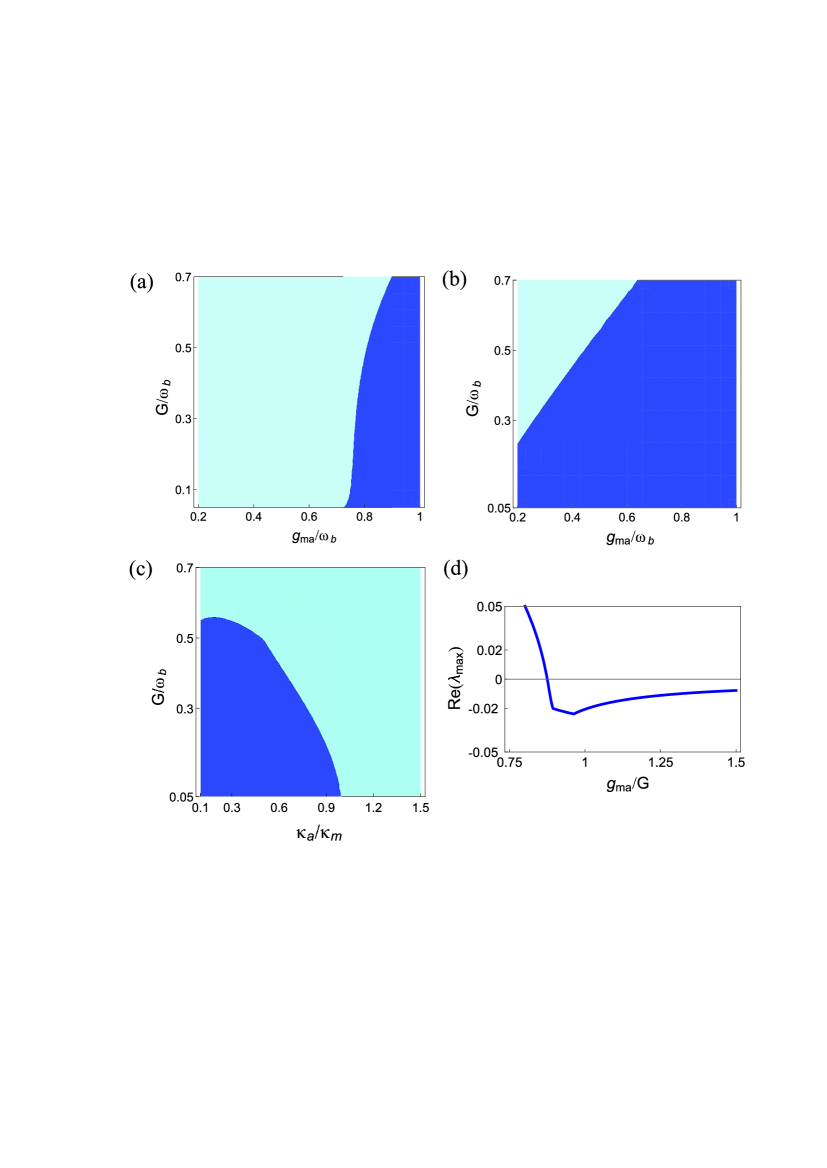
Figure 2: (a), (b) and (c) The boundary of linear stability. The light(dark) areas stands for the evolution of the system is unstable(stable). (a) The conventional CMM system $\kappa_{a}=$ $-0.2\kappa_{m}$; (b) the active-passive CMM system $\kappa_{a}=$ $0.2\kappa_{m}$. (c) The stability boundary as the system closer to the balanced gain and loss limit. $g_{ma}=0.5\omega_{b}$. (d) The maximal Lyapunov exponent as function of the ratio of $g_{ma}/G$ ($G$ is fixed) $G=0.4\omega_{b}$, $\kappa_{a}=$ $0.2\kappa_{m}$. The parameters we used are $\omega_{b}/2\pi=10MHz$, $\Delta_{a}=\tilde{\Delta}_{m}=-\omega_{b}$, $\kappa_{m}=0.1\omega_{b}$.

IV Entanglement And Steering

Here, we choose the logarithmic negativity $E_{\mathcal{N}}$ to measure the bipartite entanglements of the system Adesso et al. (2004). $E_{\mathcal{N}}$ can be computed by the quantum fluctuations of the system’s quadratures Vitali et al. (2007). Then the quadratures of the quantum fluctuations are introduced, the vector of quadratures is given by $u(t)=[\delta X_{1},\delta X_{2},\delta Y_{1},\delta Y_{2},\delta x,\delta p]^{T}$ and the vector of noise is $n(t)=[\sqrt{2\kappa_{a}}X_{1}^{in}(t),\sqrt{2\kappa_{a}}X_{2}^{in}(t),\sqrt{2\kappa_{m}}y_{1}^{in}(t),\sqrt{2\kappa_{m}}y_{2}^{in}(t),0,\xi(t)]^{T}$, where $\delta X_{1}=(\delta a+\delta a^{\dagger})/\sqrt{2}$, $\delta X_{2}=i(\delta a^{\dagger}-\delta a)/\sqrt{2}$, $\delta Y_{1}=(\delta m+\delta m^{\dagger})/\sqrt{2}$and $\delta Y_{2}=i(\delta m^{\dagger}-\delta m)/\sqrt{2}$. Similarly, the input noise quadratures are defined in the same way.

Eq.(2) can be written in a compact form $\dot{u}(t)=A\nu(t)+n(t)$, where the correlation matrix

$$A=\left(\begin{array}[]{cccccc}\kappa_{a}&\Delta_{a}&0&g_{ma}&0&0\\ -\Delta_{a}&\kappa_{a}&-g_{ma}&0&0&0\\ 0&g_{ma}&-\kappa_{m}&\tilde{\Delta}_{m}&-G&0\\ -g_{ma}&0&-\tilde{\Delta}_{m}&-\kappa_{m}&0&0\\ 0&0&0&0&0&\omega_{b}\\ 0&0&0&G&-\omega_{b}&-\gamma_{b}\end{array}\right).$$ (8)

Due to the dynamics of the system is linearized and the input noise operators $\xi$, $m^{in}$ and $a^{in}$ are Gaussian noise, the steady-state of the quantum fluctuations is a continuous variable (CV) three-mode Gaussian state. It can be obtained by a $6\times 6$ steady-state covariance matrix (CM) $V$, which can be solved by the Lyapunov equation, i.e., Vitali et al. (2007)

$$AV+VA^{T}=-D,$$ (9)

where the elements of the diffusion matrix $D$ are defined by $\delta(t-t^{{}^{\prime}})D_{i,j}=\left\langle n_{i}(t)n_{j}(t^{{}^{\prime}})+n_{j}(t^{{}^{\prime}})n_{i}(t)\right\rangle/2$. From the input noise correlation functions, one obtains $D=diag[\kappa_{a}(2n_{a}+1)$, $\kappa_{a}(2n_{a}+1)$, $\kappa_{m}(2n_{m}+1)$, $\kappa_{m}(2n_{m}+1)$, $0$, $\gamma_{b}(2n_{b}+1)]$.

In the CV case, $E_{\mathcal{N}}$ can be defined as

$$E_{\mathcal{N}}=\max[0,-\ln 2\eta^{-}],$$ (10)

where $\eta^{-}=2^{-1/2}\{\Sigma(V)-[\Sigma(V)^{2}-4\det V_{s}]^{1/2}\}^{1/2}$, with $\Sigma(V)=\det A+\det B-2\det C$. Here, $V_{s}$ is a reduced $4\times 4$ submatrix for the covariance matrix (CM). And the matrix elements of $V_{s}$ depend on the pairwise entanglement of two interesting modes (the photon-magnon, magnon-phonon and photon-phonon modes), it can be rewritten as

$$V=\left(\begin{array}[]{cc}A&C\\ C^{T}&B\end{array}\right).$$ (11)

As we know, the quantum steering is different from the entanglement for it has asymmetric characteristics between the parties. For the Gaussian states of the two interesting modes, a Gaussian quantum steering based on the form of quantum coherent information is introduced Kogias et al. (2015). Here, the $\chi_{1}\rightarrow$ $\chi_{2}$ steering is given by

$$S_{\chi_{1}\rightarrow\chi_{2}}=\max[0,\frac{1}{2}\ln\frac{\det A}{4\det V_{s}}],$$ (12)

where $\chi_{1}$ and $\chi_{2}$ stand for two interesting modes. A corresponding measure of Gaussian $\chi_{2}$ $\rightarrow$ $\chi_{1}$ steerability can be obtained by swapping $\chi_{1}$ and $\chi_{2}$, which can be expressed as

$$S_{\chi_{2}\rightarrow\chi_{1}}=\max[0,\frac{1}{2}\ln\frac{\det B}{4\det V_{s}}].$$ (13)

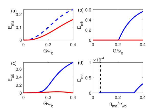
Figure 3: (a), (b) and (c) The entanglements $E_{\mathcal{N}\text{,}am}$, $E_{\mathcal{N}\text{,}bm}$ and $E_{\mathcal{N}\text{,}ab}$ as functions of the effective coupling rates $G$. The blue dotted line denotes the case of $\kappa_{a}=0.2\kappa_{m}$ (the $\mathcal{PT}$-symmetry CMM system) and the red solid line denotes the case of $\kappa_{a}=-0.2\kappa_{m}$ (the conventional CMM system). (d) The entanglements $E_{\mathcal{N}\text{,}am}$ as function of the ratio of $\kappa_{a}/\kappa_{m}(\kappa_{m}$ is fixed$)$. We set $g_{ma}=\omega_{b}$, the other parameters we chose are the same as those in Fig.2

From Fig. 3(a), (b) and (c), the bipartite entanglements $E_{\mathcal{N}\text{,}am}$, $E_{\mathcal{N}\text{,}bm}$ and $E_{\mathcal{N}\text{,}ab}$ are significantly enhanced by $\mathcal{PT}$-symmetry compared to what is generated in a conventional CMM system, where $E_{\mathcal{N}\text{,}am}$, $E_{\mathcal{N}\text{,}bm}$ and $E_{\mathcal{N}\text{,}ab}$ denote the cavity-magnon, magnon-phonon, and cavity-phonon entanglement. From Fig. 3(a), we find that with the introduction of the magnomechanical interaction, the directly coupled photons and magnons begin to entangle. In Fig. 3(b), it can be seen that the entanglement $E_{\mathcal{N}\text{,}bm}$ in the conventional CMM system is $0$. The reason is that the magnon mode driven by the blue-detuning can not cause the anti-Stokes process, which cools the mechanical mode. That is to say, the phonons cannot be cooled by the magnomechanical interaction in the conventional CMM system, thus it hinders the generation of entanglement. However, for $\mathcal{PT}$-symmetric CMM system we considered, the red-detuning driving field lead to the instability of the system. Hence, the case of blue-detuning is chosen and the strong entanglement can still be obtained in unbroken $\mathcal{PT}$-symmetry regime. Fig. 3(d) shows $E_{\mathcal{N}\text{,}am}$ versus $g_{ma}$ in the active-passive CMM system. The black vertical dotted line represents EP, which corresponds to $g_{ma}=(\kappa_{a}+\kappa_{m})/2=0.06\omega_{b}$. The entanglement occurs in the unbroken $\mathcal{PT}$-symmetry regime, and there is no entanglement in EP and broken $\mathcal{PT}$-symmetry regime. In order to make the system stable, we set $G=0.03\omega_{b}$, which leads to a very weak entanglement. In addition, the areas without solid blue lines represent that the system has no steady state.

In this work, all the results satisfy the stability conditions mentioned in the previous section. The effective magnomechanical coupling $G=4MHz$ corresponding to the drive power $27.7$mW, at the drive magnetic field $B_{0}\approx 6.88\times 10^{-5\text{ }}$and $g_{mb}=0.4Hz$ Li et al. (2018a). For this system, $G$ can be changed by adjusting the the drive power. In addition, we set $G>\kappa_{m}$ to ensure that unwanted magnon Kerr effect can be neglected in a strong magnon driving field Wang et al. (2016, 2018a).

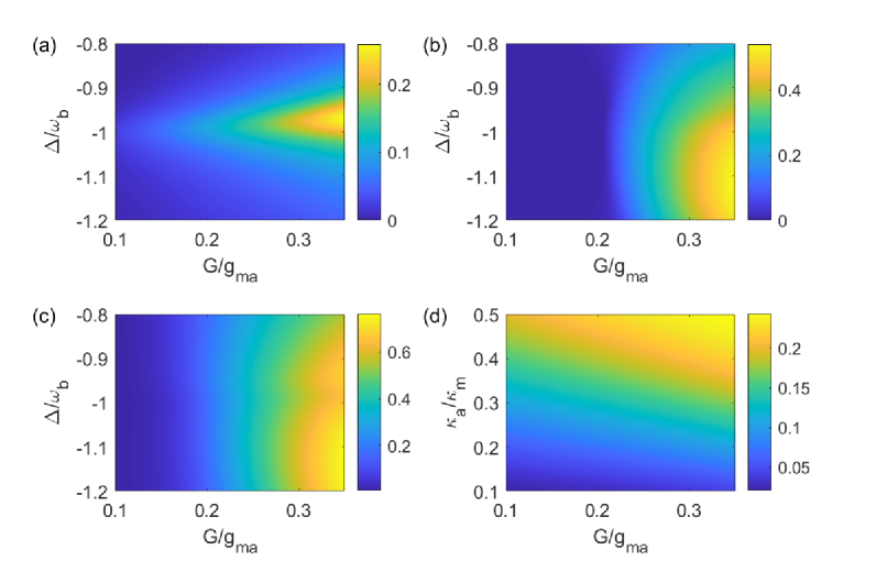
Figure 4: Density plot of the bipartite entanglement (a) $E_{\mathcal{N}\text{,}am}$, (b) $E_{\mathcal{N}\text{,}bm}$ and (c) $E_{\mathcal{N}\text{,}ab}$ versus the detuning $\Delta$ and the ratio of $G/g_{ma}$ ($g_{ma}$ is fixed). (d) Density plot of the bipartite entanglement $E_{\mathcal{N}\text{,}am}$ versus $G/g_{ma}$ ($g_{ma}$ is fixed) and $\kappa_{a}/\kappa_{m}$ ($\kappa_{m}$ is fixed). The parameters are $\kappa_{a}=0.2\kappa_{m}$, $g_{ma}=\omega_{b}$, and the other parameters we chose are the same as those in Fig.2.

In Fig. 4(a), (b) and (c), we exhibit three bipartite entanglements $E_{\mathcal{N}\text{,}am}$, $E_{\mathcal{N}\text{,}bm}$ and $E_{\mathcal{N}\text{,}ab}$ vary with the detunings $\Delta$ and the ratio of $G/g_{ma}$. As $G$ increases, the bipartite entanglements $E_{\mathcal{N}\text{,}am}$, $E_{\mathcal{N}\text{,}bm}$ and $E_{\mathcal{N}\text{,}ab}$ all increases. It can be clearly found that with the enhancement of magnomechanical interaction, the indirect photon-phonon coupling caused by magnons will also generate entanglement, and the entanglement caused by indirect coupling is larger than that caused by direct coupling, it is as mentioned in Li et al. (2018a). In addition, it shows that around $\Delta\approx-\omega_{b}$, the detuning is resonant with the mechanical sideband, the maximum entanglement $E_{\mathcal{N}\text{,}am}$ can be obtained. From Fig. 4(d), it shows the entanglement $E_{\mathcal{N}\text{,}am}$ is enhanced as the system approaches the gain-loss balance.

Fig. 5 displays the effect of $\mathcal{PT}$-symmetry on the Gaussian quantum steering. We find that the one-way quantum steering is obtained by introducing the $\mathcal{PT}$-symmetry. For the conventional CMM system, there is no quantum steering. When the system is in unbroken $\mathcal{PT}$-symmetry regime and the driving field is adjusted to make $G$ meet the required condition, there exist entangled states which are $m\rightarrow b$ and $a\rightarrow b$ one-way steerable. It is not shown in Fig. 5 that $S_{b\rightarrow m}$ and $S_{b\rightarrow a}$ are both zero under different $G$. The one-way quantum steering indicates that Bob can convince Alice that the shared state is entangled, while the converse is not true. Its application is that it provides one-side device independent quantum key distribution (QKD), where the measurement apparatus of one party only is untrusted, and it is has been experimentally observed Händchen et al. (2012); Sun et al. (2014).

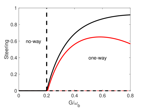
Figure 5: The quantum steerings $S_{m\rightarrow b}$ and $S_{a\rightarrow b}$ as functions of the effective coupling rates $G$. The black solid line (dotted line) denotes $S_{m\rightarrow b}$ in the $\mathcal{PT}$-symmetric CMM system (conventional CMM system), and the red solid line (dotted line) denotes $S_{a\rightarrow b}$ in the $\mathcal{PT}$-symmetric CMM system (conventional CMM system). We set $g_{ma}=\omega_{b}$ and $\kappa_{a}=$ $\pm 0.2\kappa_{m}$, the other parameters we selected are the same as those in Fig.2

It is important to discuss the influence of thermal noise on the entanglement for the quantum devices. Fig. 6 shows the robustness of the entanglement and steering against the temperature, we have plotted the entanglement and steering as the functions of the temperature $T$. In Fig. 6(a), both the entanglement and steering are discussed in unbroken $\mathcal{PT}$-symmetry regime, it can be seen that the robustness of $E_{\mathcal{N}\text{,}am}$ is better than that of $E_{\mathcal{N}\text{,}bm}$ and $E_{\mathcal{N}\text{,}ab}$, and it survives up to 180mK. The robustness of steering $S_{m\rightarrow b}$ and $S_{m\rightarrow b}$ are similar to that of $E_{\mathcal{N}\text{,}bm}$, and they all survive up to about 40mK. Then we show $\mathcal{PT}$-symmetry enhances the robustness of entanglement in Fig. 6(b), the maximum temperature of entanglement $E_{\mathcal{N}\text{,}am}$ is increased from about 147mK to 190mK.

Before ending this section, the experimental implementation is discussed. In this $\mathcal{PT}$-symmetric cavity magnomechanical system, the magnon-drive detuning can be adjusted not only by changing the frequency of the microwave driving field, but also by the frequency of the uniform magnon mode, which is modulated by an adjustable bias magnetic field $H$ in the range of 0 to 1T Wang et al. (2016). And the magnon-photon coupling can be well tuned by adjusting the bias magnetic field Yu et al. (2018). In addition, because of the material characteristics of microwave cavity, we assume that the active cavity mode can be construct by doping the active metamaterials with inherent enhancing into the cavtiy. And the assumption is based on two existing work: (1) the $\mathcal{PT}$-symmetric whispering-gallery microcavities are achieved in the experiment Peng et al. (2014). (2) a system can realize the acoustic gain by nonlinear active acoustic metamaterials Popa and Cummer (2014). For the quantum system we considered, the bipartite entanglement can be obtained by measuring the cavity field quadratures. The cavity field quadratures can be measured directly by homodyning the cavity output, and the magnon state can be measured indirectly by homodyning the cavity output of a introduced probe field. Moreover, we can used an additional optical cavity to couple the YIG sphere, so that the mechanical quadratures can be read out Li et al. (2018a, b).

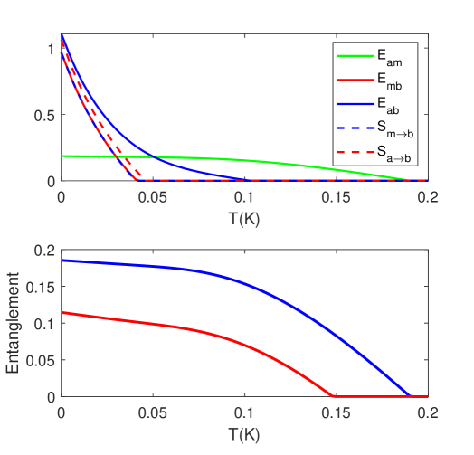
Figure 6: (a) The entanglements $E_{\mathcal{N}\text{,}am}$, $E_{\mathcal{N}\text{,}bm}$, $E_{\mathcal{N}\text{,}ab}$ and steering $S_{m\rightarrow b}$, $S_{a\rightarrow b}$ as functions of the temperature $T$, $\kappa_{a}=$ $0.2\kappa_{m}$. (b) The entanglements $E_{\mathcal{N}\text{,}am}$ as functions of the temperature $T$. The blue (red) solid line denotes the case of $\mathcal{PT}$-symmetric CMM system $\kappa_{a}=$ $0.2\kappa_{m}$ (conventional CMM system $\kappa_{a}=$ $-0.2\kappa_{m}$). We set $g_{ma}=\omega_{b}$, the other parameters we selected are the same as those in Fig.2

V Conclusions

In summary, we have investigated the enhancement of the bipartite entanglement in a $\mathcal{PT}$-symmetric CMM system. By calculating linear stability of the system, we find that the stability of the system decreases with the system approaches the gain-loss balance. Compared with the cases of broken $\mathcal{PT}$-symmetry and conventional CMM systems, the unbroken $\mathcal{PT}$-symmetric system is more stable in the range of parameters we consider. Then we show that the bipartite entanglement and the robustness of entanglement against environmental temperature are obviously enhanced by $\mathcal{PT}$-symmetry through comparison of the conventional CMM system. By selecting appropriate driving field, one-way quantum steering between magnon-phonon and photon-phonon modes can be observed by introducing $\mathcal{PT}$-symmetry. The experimental implementation is also discussed. We believe that the proposed scheme provides a method for the entanglement generation and the control of quantum steering in present cavity optomechanics and it has potential applications in quantum optical devices and quantum information networks.

References

- Huebl et al. (2013) Hans Huebl, Christoph W. Zollitsch, Johannes Lotze, Fredrik Hocke, Moritz Greifenstein, Achim Marx, Rudolf Gross, and Sebastian T. B. Goennenwein, “High cooperativity in coupled microwave resonator ferrimagnetic insulator hybrids,” Phys. Rev. Lett. 111, 127003 (2013).
- Zhang et al. (2014) Xufeng Zhang, Chang-Ling Zou, Liang Jiang, and Hong X. Tang, “Strongly coupled magnons and cavity microwave photons,” Phys. Rev. Lett. 113, 156401 (2014).
- Bourhill et al. (2016) J. Bourhill, N. Kostylev, M. Goryachev, D. L. Creedon, and M. E. Tobar, “Ultrahigh cooperativity interactions between magnons and resonant photons in a yig sphere,” Phys. Rev. B 93, 144420 (2016).
- Zhang et al. (2015a) Dengke Zhang, Xinming Wang, Tiefu Li, Xiaoqing Luo, Weidong Wu, Franco Nori, and J Q You, “Cavity quantum electrodynamics with ferromagnetic magnons in a small yttrium-iron-garnet sphere,” npj Quantum Information 1, 15014 (2015a).
- Aspelmeyer et al. (2014) Markus Aspelmeyer, Tobias J. Kippenberg, and Florian Marquardt, “Cavity optomechanics,” Rev. Mod. Phys. 86, 1391–1452 (2014).
- Zeng et al. (2020) Ye-Xiong Zeng, Jian Shen, Ming-Song Ding, and Chong Li, “Macroscopic schrödinger cat state swapping in optomechanical system,” Opt. Express 28, 9587–9602 (2020).
- Xiong et al. (2020) Biao Xiong, Xun Li, Shilei Chao, Zhen Yang, Wenzhao Zhang, Weiping Zhang, and Ling Zhou, “Strong mechanical squeezing in an optomechanical system based on lyapunov control,” Photonics Research 8, 151–159 (2020).
- Zhang et al. (2019) Wen-Zhao Zhang, Li-Bo Chen, Jiong Cheng, and Yun-Feng Jiang, “Quantum-correlation-enhanced weak-field detection in an optomechanical system,” Phys. Rev. A 99, 063811 (2019).
- Liao et al. (2020) Chang-Geng Liao, Hong Xie, Rong-Xin Chen, Ming-Yong Ye, and Xiu-Min Lin, “Controlling one-way quantum steering in a modulated optomechanical system,” Phys. Rev. A 101, 032120 (2020).
- Zeng et al. (2019) Yexiong Zeng, Tesfay Gebremariam, Mingsong Ding, and Chong Li, “The influence of non‐markovian characters on quantum adiabatic evolution,” Annalen der Physik 531, 1800234 (2019).
- Zhang et al. (2015b) Xufeng Zhang, Chang-Ling Zou, Liang Jiang, and Hong Tang, “Cavity magnomechanics,” Science Advances 2 (2015b), 10.1126/sciadv.1501286.
- Wang et al. (2018a) Yi-Pu Wang, Guo-Qiang Zhang, Dengke Zhang, Tie-Fu Li, C.-M. Hu, and J. Q. You, “Bistability of cavity magnon polaritons,” Phys. Rev. Lett. 120, 057202 (2018a).
- Li et al. (2018a) Jie Li, Shi-Yao Zhu, and G. S. Agarwal, “Magnon-photon-phonon entanglement in cavity magnomechanics,” Phys. Rev. Lett. 121, 203601 (2018a).
- Liu et al. (2018) Zengxing Liu, Bao Wang, Hao Xiong, and Ying Wu, “Magnon-induced high-order sideband generation,” Optics Letters 43, 3698–3701 (2018).
- Wang et al. (2016) Yi-Pu Wang, Guo-Qiang Zhang, Dengke Zhang, Xiao-Qing Luo, Wei Xiong, Shuai-Peng Wang, Tie-Fu Li, C.-M. Hu, and J. Q. You, “Magnon kerr effect in a strongly coupled cavity-magnon system,” Phys. Rev. B 94, 224410 (2016).
- Wang et al. (2018b) Bao Wang, Zeng-Xing Liu, Cui Kong, Hao Xiong, and Ying Wu, “Magnon-induced transparency and amplification in pt-symmetric cavity-magnon system,” Optics Express 26, 20248 (2018b).
- Woods (2001) L. M. Woods, “Magnon-phonon effects in ferromagnetic manganites,” Phys. Rev. B 65, 014409 (2001).
- Gao et al. (2017) Yong-Pan Gao, Cong Cao, Tie-Jun Wang, Yong Zhang, and Chuan Wang, “Cavity-mediated coupling of phonons and magnons,” Phys. Rev. A 96, 023826 (2017).
- Wang et al. (2020) Liang Wang, Zhi‐Xin Yang, Yu‐Mu Liu, Cheng Hua Bai, Dong-Yang Wang, Shou Zhang, and Hong-Fu Wang, “Magnon blockade in a ‐symmetric‐like cavity magnomechanical system,” Annalen der Physik , 2000028 (2020).
- Yuan et al. (2020) H. Y. Yuan, Shasha Zheng, Zbigniew Ficek, Q. Y. He, and Man-Hong Yung, “Enhancement of magnon-magnon entanglement inside a cavity,” Phys. Rev. B 101, 014419 (2020).
- Huai et al. (2019) Sai-Nan Huai, Yu-Long Liu, Jing Zhang, Lan Yang, and Yu-xi Liu, “Enhanced sideband responses in a pt-symmetric-like cavity magnomechanical system,” Phys. Rev. A 99, 043803 (2019).
- Ding and Li (2019a) Ming-Song Ding and C. Li, “Phonon laser in a cavity magnomechanical system,” Scientific Reports 9, 15723 (2019a).
- Ding and Li (2019b) Ming-Song Ding and C. Li, “Ground-state cooling of a magnomechanical resonator induced by magnetic damping,” Journal of the Optical Society of America B 37 (2019b), 10.1364/JOSAB.380755.
- Zhao et al. (2020) Chengsong Zhao, Xun Li, Shilei Chao, Rui Peng, Chong Li, and Ling Zhou, “Simultaneous blockade of a photon, phonon, and magnon induced by a two-level atom,” Phys. Rev. A 101, 063838 (2020).
- Gao et al. (2019) Yong-Pan Gao, Xiao-Fei Liu, Tie-Jun Wang, Cong Cao, and Chuan Wang, “Photon excitation and photon-blockade effects in optomagnonic microcavities,” Phys. Rev. A 100, 043831 (2019).
- Chong et al. (2011) Y. D. Chong, Li Ge, and A. Douglas Stone, “-symmetry breaking and laser-absorber modes in optical scattering systems,” Phys. Rev. Lett. 106, 093902 (2011).
- Bender and Boettcher (1998) Carl M. Bender and Stefan Boettcher, “Real spectra in non-hermitian hamiltonians having pt symmetry,” Phys. Rev. Lett. 80, 5243–5246 (1998).
- Jing et al. (2014) Hui Jing, S. K. Özdemir, Xin-You Lü, Jing Zhang, Lan Yang, and Franco Nori, “-symmetric phonon laser,” Phys. Rev. Lett. 113, 053604 (2014).
- Peng et al. (2014) Bo Peng, Sahin Kaya Ozdemir, Fuchuan Lei, Faraz Monifi, Mariagiovanna Gianfreda, Guilu Long, Shanhui Fan, Franco Nori, Carl M Bender, and Lan Yang, “Parity–time-symmetric whispering-gallery microcavities,” Nature Physics 10, 394–398 (2014).
- Liu et al. (2016) Zhong-Peng Liu, Jing Zhang, Şahin Kaya Özdemir, Bo Peng, Hui Jing, Xin-You Lü, Chun-Wen Li, Lan Yang, Franco Nori, and Yu-xi Liu, “Metrology with -symmetric cavities: Enhanced sensitivity near the -phase transition,” Phys. Rev. Lett. 117, 110802 (2016).
- Lü et al. (2015) Xin-You Lü, Hui Jing, Jin-Yong Ma, and Ying Wu, “-symmetry-breaking chaos in optomechanics,” Phys. Rev. Lett. 114, 253601 (2015).
- Li et al. (2015a) Jiahua Li, Xiaogui Zhan, Chunling Ding, Duo Zhang, and Ying Wu, “Enhanced nonlinear optics in coupled optical microcavities with an unbroken and broken parity-time symmetry,” Phys. Rev. A 92, 043830 (2015a).
- Liu et al. (2017) Yu-Long Liu, Rebing Wu, Jing Zhang, Şahin Kaya Özdemir, Lan Yang, Franco Nori, and Yu-xi Liu, “Controllable optical response by modifying the gain and loss of a mechanical resonator and cavity mode in an optomechanical system,” Phys. Rev. A 95, 013843 (2017).
- Li et al. (2017) Wenlin Li, Chong Li, and Heshan Song, “Theoretical realization and application of parity-time-symmetric oscillators in a quantum regime,” Phys. Rev. A 95, 023827 (2017).
- Makris et al. (2008) K. G. Makris, R. El-Ganainy, D. N. Christodoulides, and Z. H. Musslimani, “Beam dynamics in symmetric optical lattices,” Phys. Rev. Lett. 100, 103904 (2008).
- Tchodimou et al. (2017) C. Tchodimou, P. Djorwe, and S. G. Nana Engo, “Distant entanglement enhanced in -symmetric optomechanics,” Phys. Rev. A 96, 033856 (2017).
- El-Ganainy et al. (2018) Ramy El-Ganainy, Konstantinos Makris, Mercedeh Khajavikhan, Ziad Musslimani, Stefan Rotter, and Demetrios Christodoulides, “Non-hermitian physics and pt symmetry,” Nature Physics 14, 11–19 (2018).
- Xu et al. (2020) Wen-Ling Xu, Xiao-Fei Liu, Yang Sun, Yong-Pan Gao, Tie-Jun Wang, and Chuan Wang, “Magnon-induced chaos in an optical -symmetric resonator,” Phys. Rev. E 101, 012205 (2020).
- Adesso et al. (2004) Gerardo Adesso, Alessio Serafini, and Fabrizio Illuminati, “Extremal entanglement and mixedness in continuous variable systems,” Phys. Rev. A 70, 022318 (2004).
- Zhang et al. (2017) X. Y. Zhang, Y. Q. Guo, P. Pei, and X. X. Yi, “Optomechanically induced absorption in parity-time-symmetric optomechanical systems,” Phys. Rev. A 95, 063825 (2017).
- Lathrop (2015) Daniel Lathrop, “Nonlinear dynamics and chaos: With applications to physics, biology, chemistry, and engineering,” Physics Today 68, 54–55 (2015).
- Benettin et al. (1980) Giancarlo Benettin, L. Galgani, Antonio Giorgilli, and Marie Strelcyn, “Lyapunov characteristic exponents for smooth dynamical systems and for hamiltonian systems; a method for computing all of them. part 1: theory.” Meccanica 15, 9–20 (1980).
- Lü et al. (2015) Ling Lü, Chengren Li, Shuo Liu, Zhouyang Wang, Jing Tian, and Jiajia Gu, “The signal synchronization transmission among uncertain discrete networks with different nodes,” Nonlinear Dynamics 81 (2015), 10.1007/s11071-015-2030-4.
- Li et al. (2015b) Wenlin Li, Chong Li, and Heshan Song, “Quantum parameter identification of a chaotic atom ensemble system,” Physics Letters A 380 (2015b), 10.1016/j.physleta.2015.06.055.
- Vitali et al. (2007) D. Vitali, S. Gigan, A. Ferreira, H. R. Böhm, P. Tombesi, A. Guerreiro, V. Vedral, A. Zeilinger, and M. Aspelmeyer, “Optomechanical entanglement between a movable mirror and a cavity field,” Phys. Rev. Lett. 98, 030405 (2007).
- Kogias et al. (2015) Ioannis Kogias, Antony R. Lee, Sammy Ragy, and Gerardo Adesso, “Quantification of gaussian quantum steering,” Phys. Rev. Lett. 114, 060403 (2015).
- Händchen et al. (2012) Vitus Händchen, Tobias Gehring, Sebastian Steinlechner, Aiko Samblowski, Torsten Franz, Reinhard Werner, and Roman Schnabel, “Observation of one-way einstein-podolsky-rosen steering,” Nature Photonics 6 (2012), 10.1038/nphoton.2012.202.
- Sun et al. (2014) Kai Sun, Jin-Shi Xu, Xiang-Jun Ye, Yu-Chun Wu, Jing-Ling Chen, Chuan-Feng Li, and Guang-Can Guo, “Experimental demonstration of the einstein-podolsky-rosen steering game based on the all-versus-nothing proof,” Phys. Rev. Lett. 113, 140402 (2014).
- Yu et al. (2018) Haiming Yu, Jiang Xiao, and Philipp Pirro, ““magnon spintronics”,” Journal of Magnetism and Magnetic Materials 450, 1–2 (2018).
- Popa and Cummer (2014) Bogdan-Ioan Popa and Steven Cummer, “Non-reciprocal and highly nonlinear active acoustic metamaterials,” Nature communications 5, 3398 (2014).
- Li et al. (2018b) Jie Li, Simon Gröblacher, Shi-Yao Zhu, and G. S. Agarwal, “Generation and detection of non-gaussian phonon-added coherent states in optomechanical systems,” Phys. Rev. A 98, 011801 (2018b).