Nighttime Dehazing with a Synthetic Benchmark

Abstract.

Increasing the visibility of nighttime hazy images is challenging because of uneven illumination from active artificial light sources and haze absorbing/scattering. The absence of large-scale benchmark datasets hampers progress in this area. To address this issue, we propose a novel synthetic method called 3R to simulate nighttime hazy images from daytime clear images, which first reconstructs the scene geometry, then simulates the light rays and object reflectance, and finally renders the haze effects. Based on it, we generate realistic nighttime hazy images by sampling real-world light colors from a prior empirical distribution. Experiments on the synthetic benchmark show that the degrading factors jointly reduce the image quality. To address this issue, we propose an optimal-scale maximum reflectance prior to disentangle the color correction from haze removal and address them sequentially. Besides, we also devise a simple but effective learning-based baseline which has an encoder-decoder structure based on the MobileNet-v2 backbone. Experiment results demonstrate their superiority over state-of-the-art methods in terms of both image quality and runtime. Both the dataset and source code will be available at https://github.com/chaimi2013/3R.

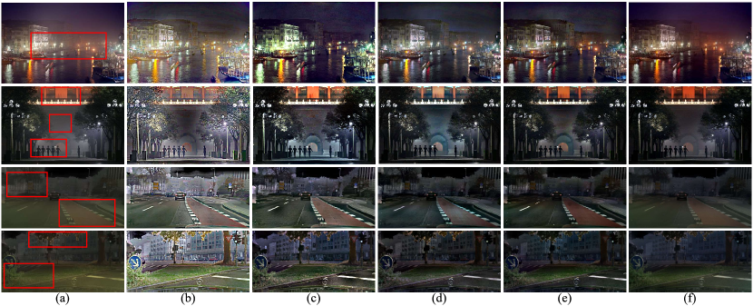
Figure 1. (a) Nighttime hazy images. (b) NDIM (Zhang et al., 2014). (c) GS (Li et al., 2015). (d) MRP (Zhang et al., 2017). (e) Our OSFD. (f) Our ND-Net.

1. Introduction

In contrast to daytime imaging conditions, where the illumination is dominated by global uniform atmospheric light, nighttime illumination is mainly from active, synthetic light sources such as street and neon lights. These lights are located at different positions, have limited illumination range, and produce diverse colors, resulting in a low-visibility image with uneven illumination and color cast. If the conditions are hazy, image visibility will be even worse, since haze degrades image contrast through absorption and scattering (see examples in Figure 1(a)). Removing color cast and haze is crucial for increasing the visibility of nighttime hazy images, which, however, is very challenging due to its ill-posed nature.

To address this problem, Pei and Lee first proposed a color-transfer technique to convert a nighttime hazy image into a grayish one by referring to the color statistics of a reference daytime image (Pei and Lee, 2012). While reducing the color cast, it also changed the original color distribution and generated unrealistic results with color artifacts (Zhang et al., 2017). Zhang $et~{}al.$ proposed a model-based method to correct the color cast (Zhang et al., 2014) and remove haze using the dark channel prior (He et al., 2009). However, the light compensation added extra color cast that affected the subsequent color correction (Figure 1(b)). Li $et~{}al.$ proposed a layer separation algorithm to remove the glow of light sources in the input image (Li et al., 2015). While producing better haze-free images than previous methods, it also generated some color artifacts around the light sources and amplified noise (Figure 1(c)). Recently, Zhang $et~{}al.$ proposed a statistical prior, the maximum reflectance prior (MRP), to help remove the color cast and then dehaze (Zhang et al., 2017). However, MRP was used within each pixel’s fixed-sized neighborhood and could not adapt to diverse local statistics such as large areas of the monochromatic lawn (Figure 1(d)).

Less progress has been made in nighttime dehazing than daytime dehazing, especially in the context of deep learning. For example, many convolutional neural networks (CNN)-based methods have been proposed for daytime dehazing (Cai et al., 2016; Ren et al., 2016, 2016; Li et al., 2017; Ren et al., 2018; Zhang and Patel, 2018; Yang and Sun, 2018; Zhang et al., 2018; Li et al., 2019; Deng et al., 2019; Liu et al., 2019; Zhang and Tao, 2020; Wang et al., 2020). The benefit of the strong representation capacity of CNN relies on large-scale training data. Even when trained on synthetic images, they show good generalization ability to real-world daytime hazy images. However, this is not the case for nighttime hazy scenarios. First, models trained on synthetic daytime hazy images do not generalize well to nighttime hazy images due to the illumination discrepancy. Second, synthesizing nighttime hazy images is not straightforward due to the spatially variant illumination and its entanglement with haze scattering and absorption.

To address this issue, we propose a novel synthetic method to simulate nighttime hazy images from daytime clear images called 3R. We first conduct an empirical study on real-world light colors to obtain a prior distribution. Then, we use 3R to synthesize realistic nighttime hazy images by sampling real-world light colors. Specifically, it first reconstructs the scene geometry, then simulates the light rays and object reflectance, and finally renders the haze effects. We build a new synthetic dataset to benchmark state-of-the-art (SOTA) methods. As noted above, existing methods suffer from the entanglement of both degrading factors, i.e., active light sources and haze. To address this issue, we propose an optimal-scale maximum reflectance prior (OS-MRP) to disentangle the color correction from haze removal and address them sequentially (Figure 1(e)). Also, we devise a new CNN baseline model with an encoder-decoder structure, which also achieves good performance at high computational efficiency (Figure 1(f)). The main contributions of this paper are:

$\bullet$ We propose a novel synthetic method to establish a benchmark and evaluate SOTA nighttime dehazing methods comprehensively;

$\bullet$ We derive a novel OS-MRP prior that can adapt to diverse local statistics in natural images, resulting in a computationally efficient dehazing algorithm for removing color cast and haze effectively;

$\bullet$ We devise a deep CNN model, which serves as a strong baseline and achieves good performance for nighttime dehazing;

$\bullet$ Extensive experiments on synthetic datasets and real-world images demonstrate the superiority of the proposed methods in terms of both image quality and runtime.

2. Related work

(1) $$\bm{{\rm{I}}}\left(\bm{{\rm{x}}}\right) ={L}\left(\bm{{\rm{x}}}\right)\bm{{\rm{\eta}}}\left(\bm{{\rm{x}}}\right)\bm{{\rm{R}}}\left(\bm{{\rm{x}}}\right)t\left(\bm{{\rm{x}}}\right)+{L}\left(\bm{{\rm{x}}}\right)\bm{{\rm{\eta}}}\left(\bm{{\rm{x}}}\right)\left({1-t\left(\bm{{\rm{x}}}\right)}\right)$$

$$\buildrel\Delta\over{=}\bm{{\rm{J}}}\left(\bm{{\rm{x}}}\right)\bm{{\rm{\eta}}}\left(\bm{{\rm{x}}}\right)t\left(\bm{{\rm{x}}}\right)+{L}\left(\bm{{\rm{x}}}\right)\bm{{\rm{\eta}}}\left(\bm{{\rm{x}}}\right)\left({1-t\left(\bm{{\rm{x}}}\right)}\right),$$

The nighttime imaging model can be formulated as above by referring to (Zhang et al., 2017). Here, $\bm{{\rm{I}}}\left(\bm{{\rm{x}}}\right)$ is the nighttime hazy image, ${L}\left(\bm{{\rm{x}}}\right)$ and $\bm{{\rm{\eta}}}\left(\bm{{\rm{x}}}\right)$ are the illuminance and color cast from active light sources, $\bm{{\rm{R}}}\left(\bm{{\rm{x}}}\right)$ is the reflectance, $t\left(\bm{{\rm{x}}}\right)$ is the haze transmission, and $\bm{{\rm{J}}}\left(\bm{{\rm{x}}}\right)$ is the nighttime clear image:

(2) $$\bm{{\rm{J}}}\left(\bm{{\rm{x}}}\right)\buildrel\Delta\over{=}\bm{{\rm{R}}}\left(\bm{{\rm{x}}}\right){L}\left(\bm{{\rm{x}}}\right),$$

where $\bm{{\rm{x}}}$ is the pixel index. Recovering $\bm{{\rm{J}}}$ from $\bm{{\rm{I}}}$ is a typical ill-posed problem relying on the estimation of latent ${L}$, $\bm{{\rm{\eta}}}$, and $t$. Previous work either used statistical priors to regularize the optimization or learned the latent variables or $\bm{{\rm{J}}}$ from the training data directly.

Image dehazing with statistical priors: For the daytime case, $L\bm{{\rm{\eta}}}$ is global constant atmospheric light. Therefore, the primary target is to estimate haze transmission. To this end, different statistical priors have been proposed (He et al., 2009; Fattal, 2014; Zhu et al., 2015; Berman et al., 2016) including the dark channel prior (DCP) (He et al., 2009). However, these cannot be directly used for nighttime dehazing. For instance, DCP is no longer valid in the nighttime case where the color cast from active light sources biases the dark channel. To address this issue, previous methods have decomposed nighttime dehazing into two steps: color cast correction and haze removal (Pei and Lee, 2012; Zhang et al., 2014; Li et al., 2015; Ancuti et al., 2016; Zhang et al., 2017). Correcting the color cast, also known as color constancy, is very well studied (Buchsbaum, 1980; Van De Weijer et al., 2007; Joze et al., 2012; Barron, 2015; Barron and Tsai, 2017; Hu et al., 2017). However, color cast is usually a global constant which differs from the spatially variant one in the nighttime dehazing case. Li $et~{}al.$ estimated the local color cast using the brightest pixel prior (Joze et al., 2012) in each local patch. However, the bright pixel within a local patch may not be white, resulting in a biased estimate towards the image’s intrinsic color. MRP in (Zhang et al., 2017) instead used the maximum reflectance in each channel separately, $i.e.$, they were not necessarily from the same pixel. Nevertheless, it may fail in monochromatic areas such as the lawn. By contrast, we propose a novel optimal-scale maximum reflectance prior, which can adapt to diverse local statistics.

Image dehazing by supervised learning: Supervised learning-based image dehazing methods (Cai et al., 2016; Ren et al., 2016; Li et al., 2017; Ren et al., 2018; Zhang and Patel, 2018; Yang and Sun, 2018; Zhang et al., 2018; Li et al., 2019; Deng et al., 2019; Zhang and Tao, 2020) need large-scale paired training samples. Daytime dehazing methods synthesize hazy samples from clear ones according to the imaging model, where the transmission is either assumed to be a constant within each local patch (Tang et al., 2014; Cai et al., 2016) or calculated from the scene depth (Ren et al., 2016; Li et al., 2017, 2018; Sakaridis et al., 2018). Recently, Ancuti $et~{}al.$ collected real hazy and corresponding haze-free images in both outdoor and indoor scenes and constructed the O-Haze (45 pairs) and IHaze (35 pairs) datasets (Ancuti et al., 2018b, a). However, collecting nighttime hazy images is non-trivial due to the need for long exposures, static scenes, and illumination calibration. Instead, Zhang $et~{}al.$ (Zhang et al., 2017) synthesized nighttime hazy images based on the Middlebury datasets (Scharstein and Szeliski, 2003) by assuming a single central light source with a constant yellow color, which limited the sampling space. By contrast, we carry out an empirical study on real-world light colors to obtain their distribution. Then, we propose a novel synthetic method by further taking the scene geometry into account. It can generate realistic nighttime hazy images by rendering the spatially variant color cast and haze simultaneously.

3. Synthetic nighttime hazy images

3.1. Empirical study on real-world light colors

Before synthesizing nighttime images, we must first understand real-world light colors. To this end, we collected over 1,300 real-world nighttime images from the internet using search terms such as “nighttime road”, ”street light”, $etc$. Some examples are shown in Figure 2. Generally, the dominant illumination is from artificial active lights. Therefore, we used them to calculate the prior distribution of light colors. First, they were resized into 100x100. Then, different scales of patches were densely sampled from them, ranging from 11x11 to 100x100 pixels. At each patch, we used MRP to estimate its color cast. The results are plotted as black scattered dots in Figure 2. Note that we assume the red channel is 1 since the light colors are biased to warm colors. At each scale, we calculated the mean (center) and the standard deviation of all samples as shown in the purple circles. We then used linear regression to fit these centers and obtain a prior equation of the light colors, $i.e.$,

(3) $$Blue=Green\times 1.133-0.3616.$$

Then, we shifted the line upwards and downwards according to the standard deviations to determine the boundaries, as shown by the red dotted lines; the region bounded by them covered 98.68% of samples. Next, we calculated the distribution of green values as shown in the green histograms. According to this distribution and Eq. (3), we randomly sampled light colors inside the boundaries, which are plotted as red dots and visualized in the upper left corner. They are visually realistic and mimic real-world light colors.

3.2. A novel synthetic method: 3R

Different from (Zhang et al., 2017), where the illuminance is calculated from the light path distance via an exponential decay model, we follow the inverse-square law (Millerson, 2013, p. 26) and Lambert’s cosine law (Basri and Jacobs, 2003) to calculate the illuminance from the light path distance, incident light direction, and surface normal direction. Therefore, we should first reconstruct scene geometry by calculating the surface normals.

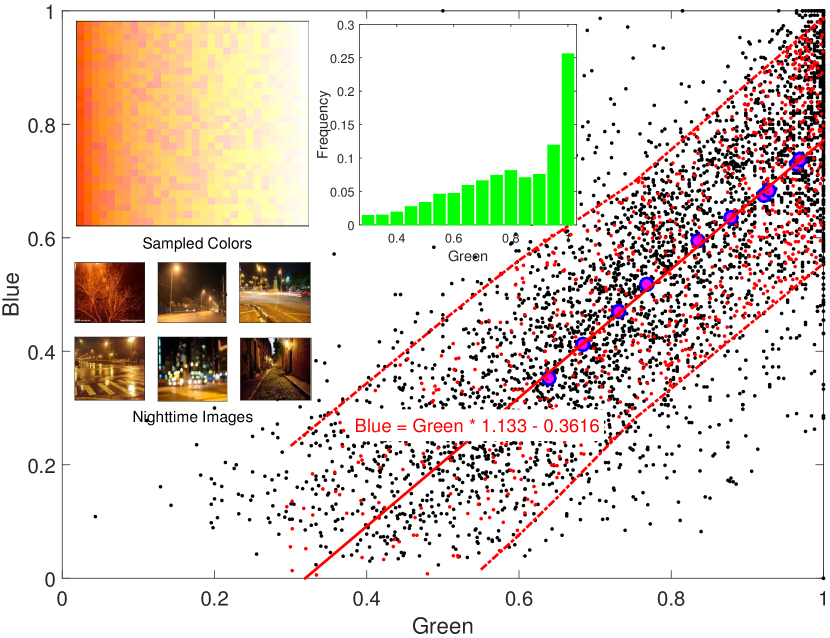
Figure 2. Empirical study on the real-world light colors.

Scene reconstruction: Taking the Cityscapes dataset (Cordts et al., 2016) as an example, given a clear image $\bm{{\rm{R}}}$, semantic labels $C$, and depth map ${D}$, our target is to synthesize a realistic nighttime hazy image. First, we use SLIC (Achanta et al., 2012) to segment the semantic label into super-pixels. After calculating the world coordinates $\bm{{\rm{x_{i}}}}$ of pixels on each super-pixel $\bm{{\rm{z}}}$ based on the depth and camera parameters, a 3d plane is fitted to obtain the normal vector $\bm{{\rm{v\left(\bm{{\rm{z}}}\right)}}}$ and bias $m$ according to:

(4) $$\bm{{\rm{v\left(\bm{{\rm{z}}}\right)}}}=\mathop{\min}\limits_{\bm{{\rm{v}}}}\sum\limits_{i}{{{\left\|{{\bm{{\rm{v}}}^{T}}{\bm{{\rm{x_{i}}}}}+m}\right\|}^{2}}}.$$

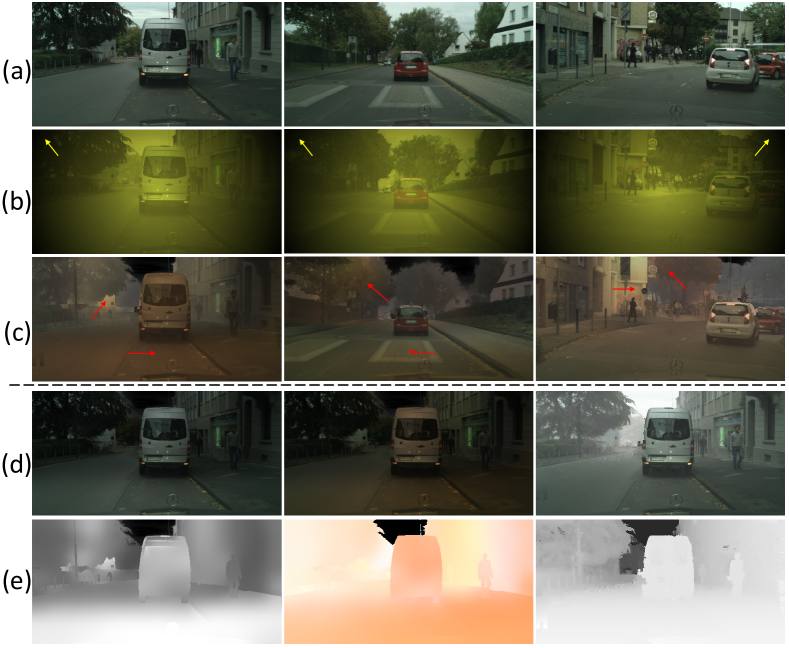
Figure 3. Examples of synthetic images. (a) Daytime clear images from the Cityscapes dataset (Cordts et al., 2016). (b) Results using the method in (Zhang et al., 2017). (c) Results using the proposed 3R. (d)-(e) Some intermediate results using 3R, $i.e.$, (d) a low-light image without/with color cast, daytime hazy image, (e) the illuminance intensity, color cast, and haze transmission.

Ray simulation: Then, the illuminance reaching $\bm{{\rm{z}}}$ from the $k^{th}$ light can be calculated according to Lambert’s cosine law (Basri and Jacobs, 2003):

(5) $$\bm{{\rm{{L_{k}}\left(\bm{{\rm{z}}}\right)}}}={\bm{{\rm{\eta_{k}}}}}\frac{{{\beta_{l}}}}{{d{{\left(\bm{{\rm{z}}}\right)}^{2}}}}{\max\left({{\bm{{\rm{u_{k}}}}}{{\left(\bm{{\rm{z}}}\right)}^{T}}\bm{{\rm{v}}}\left(\bm{{\rm{z}}}\right)},0\right)}.$$

We use the bold $\bm{{\rm{{L_{k}}}}}$ to denote the light intensity $L_{k}$ and color $\bm{{\rm{{\eta_{k}}}}}$ together. $\beta_{l}$ is a parameter, $d\left(\bm{{\rm{z}}}\right)$ is the distance between the $k^{th}$ light source and $\bm{{\rm{z}}}$, and ${{\bm{{\rm{u_{k}}}}}\left(\bm{{\rm{z}}}\right)}$ is the incident light direction from the $k^{th}$ light to $\bm{{\rm{z}}}$. Then, the illuminance from all light sources are:

(6) $$\bm{{\rm{{L}\left(\bm{{\rm{z}}}\right)}}}=\sum\limits_{k}{\bm{{\rm{{L_{k}}\left(\bm{{\rm{z}}}\right)}}}}.$$

The illuminance map is further refined using the fast guided filter (He and Sun, 2015). In our experiments, we place virtual light sources along the roadsides according to the semantic labels $C$, which are 5 meters high and spaced every 30 meters. The light colors are randomly sampled as in Section 3.1.

Rendering: The haze absorbing and scattering effects rely on haze transmission, which can be calculated from the scene depth according to exponential decay model (Sakaridis et al., 2018):

(7) $$t\left(\bm{{\rm{x}}}\right)={e^{-{\beta_{t}}d\left(\bm{{\rm{x}}}\right)}},$$

where $\beta_{t}$ is the attenuation coefficient controlling the thickness of the haze. $d\left(\bm{{\rm{x}}}\right)$ is the scene depth. Finally, we render the haze effect to generate the nighttime haze image by integrating the illuminance and transmission into Eq. (1).

In this paper, we call the above method “3R” and summarize it in Algorithm 1. As can be seen from the walls, roads, and cars in Figure 3(c), the illuminance is more realistic than Figure 3(b), since 3R leverages the scene geometry and real-world light colors. The haze further reduces image contrast, especially in distant regions. It is noteworthy that we mask out the sky region due to its inaccurate depth values. 3R also generates some intermediate results such as $L$, $\bm{{\rm{\eta}}}$, $t$, which are worthy of further study, for example for learning disentangled representations.

Input: $\bm{{\rm{R}}}$, $C$, $D$, $\beta_{l}$, $\beta_{t}$, $\left\{{{\bm{{\rm{\eta_{k}}}}}}\right\}_{k=1}^{K}$

Output: $\bm{{\rm{I}}}$

1 Scene Reconstruction:  

2       Segment $C$ into super-pixels $\left\{{\bm{{\rm{z_{1}}}},...}\right\}$;

3       Calculate the world coordinates $\bm{{\rm{x_{i}}}}$ of pixels on $\bm{{\rm{z}}}$;

4       Calculate the normal vector $\bm{{\rm{v}}}$ according to Eq. (4);

5      

6

7 Ray Simulation:  

8       Calculate the illuminance $\bm{{\rm{L_{k}}}}$ according to Eq. (5);

9       Aggregate the illuminance $\bm{{\rm{L_{k}}}}$ according to Eq. (6);

10       Calculate the transmission $t$ according to Eq. (7);

11      

12

13 Rendering:  

14       Synthesize $\bm{{\rm{I}}}$ according to Eq. (1).

15

Algorithm 1 Synthesizing Images via 3R

3.3. A novel synthetic benchmark

Following (Sakaridis et al., 2018), 550 clear images were selected from Cityscapes (Cordts et al., 2016) to synthesize nighttime hazy images using 3R. We synthesized 5 images for each of them by changing the light positions and colors, resulting in a total of 2,750 images, called “Nighttime Hazy Cityscapes” (NHC). We also altered the haze density by setting $\beta_{t}$ to 0.005, 0.01, and 0.02, resulting in different datasets denoted NHC-L, NHC-M, and NHC-D, where “L”, “M”, and “D” represent light haze, medium haze, and dense haze. Further, we also modified the method in (Zhang et al., 2017) by changing the constant yellow light color with our randomly sampled real-world light colors described in Section 3.1 and synthesized images on the Middlebury (70 images) (Scharstein and Szeliski, 2003) and RESIDE (8,970 images) datasets (Li et al., 2018). Similar to NHC, we augmented the Middlebury dataset by 5 times, resulting in a total of 350 images. They are denoted NHM and NHR, respectively. The statistics of these datasets are summarized in Table 1 in Section 6.

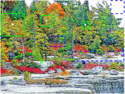
(a)

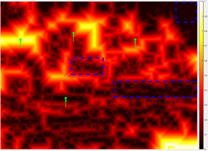
(b)

Figure 4. (a) A clear image. (b) The optimal scale map. Hot colors represent large scales. Please refer to Section 4.1.

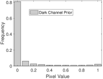
(a)

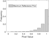
(b)

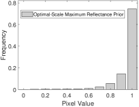
(c)

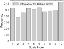
(d)

Figure 5. (a)-(d) Histograms of DCP (He et al., 2009), MRP (Zhang et al., 2017), the proposed OS-MRP, and the optimal scales in OS-MRP, respectively.

4. OS-MRP for nighttime dehazing

4.1. Optimal-scale maximum reflectance prior

Following (Zhang et al., 2017), we define the maximum reflectance $\bm{{\rm{M_{s}}}}$ of a daytime clear image patch $\bm{{\rm{R_{{\Omega_{s}}}}}}$ centered at $\bm{{\rm{x}}}$ as:

(8) $${M_{sc}\left(\bm{{\rm{x}}}\right)}=\mathop{\max}\limits_{\bm{{\rm{x}}}\in{\Omega_{s}}}{R_{c}}\left(\bm{{\rm{x}}}\right),c\in\left\{{r,g,b}\right\},$$

where $s$ is the scale of patch $\Omega_{s}$ and $\bm{{\rm{M_{s}}}}=\left[{{M_{sr}},{M_{sg}},{M_{sb}}}\right]$. In (Zhang et al., 2017), $M_{sc}$ is assumed to be close to 1 for every local patch, $i.e.$, the MRP. However, it may not hold for monochromatic areas such as lawn.

To migrate the issue, we calculate $\bm{{\rm{M_{s}}}}$ at multiple scales and determine the optimal scale for each pixel from a probability view. Specifically, we can treat the maximum reflectance as the probability of a surface patch that completely reflects incident light at all frequency range, $i.e.$,

(9) $${P_{s}}\left(\bm{{\rm{x}}}\right)=\prod\limits_{c\in\left\{{r,g,b}\right\}}{{M_{sc}\left(\bm{{\rm{x}}}\right)}}.$$

For patches containing distinct colors or bright pixels, as shown in the blue rectangles in Figure 4(a), ${P_{s}}$ of a small patch is close to 1. For some monochromatic areas, $e.g.$, the left-most green rectangle region, it needs to enlarge the patch size to include more diverse pixels. However, a large patch means a bad localization when estimating the local color cast. To address this issue, we define an optimal scale that is sufficiently large but not necessary to be larger to obtain the highest ${P_{s}}$. Since ${P_{s}}$ is a monotonically increasing function of $s$, the optimal scale is defined as:

(10) $${s^{*}}\left(\bm{{\rm{x}}}\right)=\mathop{\min}\limits_{s}\left\{{\mathop{\arg\max}\limits_{\forall s\in\mathcal{S}}{P_{s}}\left(\bm{{\rm{x}}}\right)}\right\},$$

where $\mathcal{S}$ is the set of all scales. Figure 4(b) shows the optimal scale map of (a). The optimal scales are very small for pixels with distinct colors or bright pixels. By contrast, the optimal scale is very large for monochromatic pixels. Based on the above definition, we assume:

(11) $${M_{{s^{*}}c}}\left(\bm{{\rm{x}}}\right)\approx 1,\forall c\in\left\{{r,g,b}\right\},\forall\bm{{\rm{x}}}\in{\rm\mathcal{X}},$$

where $\mathcal{X}$ is the index set of all pixels. In this paper, we call it optimal-scale maximum reflectance prior (OS-MRP).

To validate this prior, we calculated the histograms of $P_{s^{*}}$ over 1,000,000 patches sampled from daytime clear images by referring to (He et al., 2009; Zhang et al., 2017). Ten scales ranging from 7x7 to 43x43 were used when calculating $P_{s^{*}}$. A fixed scale of 25x25 was used for DCP and MRP. The results are plotted in Figure 5. Compared with MRP, more patches have the maximum reflectance in our optimal-scale case, $i.e.$, a higher bar in the last range, and lower bars in the others. Further, the optimal scale is nearly uniformly distributed as shown in Figure 5(d), implying that OS-MRP does not obtain unfair advantages from larger patches over MRP.

4.2. Nighttime dehazing

4.2.1. Initial multiscale fusion

Since ${P_{s}}\left(\bm{{\rm{x}}}\right)$ should be calculated on the clear image, we propose a novel algorithm by first dehazing using multi-scale fusion then refining it using optimal-scale fusion.

Color cast correction: Following (Zhang et al., 2017), we also assume ${L}$, $\bm{{\rm{\eta}}}$, and $t$ are constant at each local patch ${{{\Omega_{s}}}}$, $i.e.$, ${L_{s}}$, $\bm{{\rm{\eta_{s}}}}$, and $t_{s}$. Then, we calculate the maximum on ${{{\Omega_{s}}}}$ as:

(12) $$\mathop{\max}\limits_{\bm{{\rm{x}}}\in{{\Omega_{s}}}}{I_{c}}\left(\bm{{\rm{x}}}\right) ={\mathop{\max}\limits_{\bm{{\rm{x}}}\in{{\Omega_{s}}}}{R_{c}}\left(\bm{{\rm{x}}}\right)}{{L_{s}}}{{\eta_{sc}}}{t_{s}}+{{L_{s}}}{{\eta_{sc}}}\left({1-{t_{s}}}\right)$$

$$={{L_{s}}}{{\eta_{sc}}},$$

We get the last equality using MRP, $i.e.$, $\mathop{\max}\limits_{\bm{{\rm{x}}}\in{{\Omega_{s}}}}{R_{c}}\left(\bm{{\rm{x}}}\right)=1$. Given the illuminance is the maximum of all channels, $i.e.$,

(13) $$\widehat{{L_{s}}}=\mathop{\max}\limits_{c\in\left\{{r,g,b}\right\}}\mathop{\max}\limits_{\bm{{\rm{x}}}\in{{\Omega_{s}}}}{I_{c}}\left(\bm{{\rm{x}}}\right),$$

we can get the color cast accordingly,

(14) $$\widehat{{\eta_{{\rm{sc}}}}}={{\mathop{\max}\limits_{\bm{{\rm{x}}}\in{{\Omega_{s}}}}I_{c}\left(\bm{{\rm{x}}}\right)}\mathord{\left/{\vphantom{{\mathop{\max}\limits_{x\in{\Omega_{s}}}I_{c}\left(x\right)}{\widehat{{L_{s}}}}}}\right.\kern-1.2pt}{\widehat{{L_{s}}}}}.$$

We then average $\bm{{\rm{\eta_{s}}}}$ at each scale to obtain an initial estimate:

(15) $$\bm{{\rm{\widehat{\eta}}}}=\frac{1}{{\left|\mathcal{S}\right|}}\sum\limits_{s\in\mathcal{S}}\bm{{\rm{\widehat{{\eta_{s}}}}}},$$

where ${\left|\mathcal{S}\right|}$ is the number of scales. We use the fast guided filter (He and Sun, 2015) to refine $\bm{{\rm{\eta}}}$ due to its low computational cost. Then, we remove the color cast according to Eq. (1):

(16) $$\bm{{\rm{I}}}\left(\bm{{\rm{x}}}\right)=\bm{{\rm{J}}}\left(\bm{{\rm{x}}}\right)t\left(\bm{{\rm{x}}}\right)+{L}\left(\bm{{\rm{x}}}\right)\left({1-t\left(\bm{{\rm{x}}}\right)}\right).$$

Here, we reuse $\bm{{\rm{I}}}\left(\bm{{\rm{x}}}\right)$ to denote the color correction result for simplicity. Although we can average $L_{s}$ to obtain a fusion estimate like $\bm{{\rm{\eta_{s}}}}$, the illuminance intensity is less smooth than the color cast due to depth, occlusion, $etc$. Therefore, we re-estimate $L$ using MRP on Eq. (16) like in Eq. (13).

Dehazing: Given $L$, it is straightforward to obtain $t$ using the DCP (He et al., 2009) on Eq. (16), $i.e.$,

(17) $$t=1-{{\mathop{\min}\limits_{x\in{{\Omega_{t}}}}\mathop{\min}\limits_{c\in\left\{{r,g,b}\right\}}{I_{c}}\left(x\right)}\mathord{\left/{\vphantom{{\mathop{\min}\limits_{x\in{{\Omega_{t}}}}\mathop{\min}\limits_{c\in\left\{{r,g,b}\right\}}{I_{c}}\left(x\right)}{\mathop{\min}\limits_{x\in{{\Omega_{t}}}}L}}}\right.\kern-1.2pt}{\mathop{\min}\limits_{x\in{{\Omega_{t}}}}L}}\left(x\right),$$

where ${\Omega_{t}}$ is the local patch. We refine $t$ using the fast guided filter. Finally, the haze-free image is recovered as:

(18) $$\bm{{\rm{J}}}={{\left({\bm{{\rm{I}}}-L}\right)}\mathord{\left/{\vphantom{{\left({\bm{{\rm{I}}}-L}\right)}{\max\left({t,{t_{0}}}\right)+}}}\right.\kern-1.2pt}{\max\left({t,{t_{0}}}\right)+}}L,$$

where $t_{0}$ is a small threshold for numerical stability.

4.2.2. OSFD: Optimal-scale fusion-based dehazing

Based on the initial estimate $\bm{{\rm{J}}}$ and $L$, we normalize $\bm{{\rm{J}}}$ by $L$ according to Eq. (2) and calculate the optimal scale $s^{*}\left(\bm{{\rm{x}}}\right)$ at all pixels according to Eq. (8) $\sim$ Eq. (10). The optimal scale can be regarded as the “best” patch size on which to estimate the color cast, where there are sufficient maximum reflectance pixels to be used. Therefore, we propose the following optimal-scale fusion to estimate the color cast:

(19) $$\bm{{\rm{\widehat{\eta}}}}=\sum\limits_{s\in\mathcal{S}}{{\delta_{{s^{*}}s}}\bm{{\rm{\widehat{{\eta_{s}}}}}}},$$

where ${\delta_{{s^{*}}s}}$ is the Kronecker delta function, $i.e.$, ${\delta_{{s^{*}}s}}=1$ if $s^{*}=s$, otherwise 0. After obtaining $\bm{{\rm{\eta}}}$, we remove the color cast and haze according to Eq. (16) $\sim$ Eq. (18).

4.3. Computational complexity analysis

There are two kinds of basic operation in OSFD: the patch-wise max, min, sum, and the pixel-wise sum, multiplication, division. To avoid the dense patch-wise max and min, we adopt an overlapping sliding window algorithm, reducing the complexity from $\mathcal{O}\left(r^{2}N\right)$ to $\mathcal{O}\left(N\right)$. $r$ is the patch radius. $N$ is the number of pixels. The stride of the sliding window is $r$. For the patch-wise sum, we follow (He and Sun, 2015) and use the summed-area table algorithm, reducing the complexity from $\mathcal{O}\left(r^{2}N\right)$ to $\mathcal{O}\left(N\right)$. Moreover, compared with the original guided filter (He et al., 2010), the computational complexity of the fast guided filter is reduced from $\mathcal{O}\left(N\right)$ to $\mathcal{O}\left({N\mathord{\left/{\vphantom{N{{d^{2}}}}}\right.\kern-1.2pt}{{d^{2}}}}\right)$, where $d$ is the sub-sampling ratio. Therefore, considering that $\bm{{\rm{\eta_{s}}}}$ is calculated at all $\left|S\right|$ scales, the total computational complexity of OSFD is $\mathcal{O}\left(\left|\mathcal{S}\right|N\right)$. Further, we down-sample the image $\bm{{\rm{I}}}$ by a ratio $k_{s}$ when calculating $\bm{{\rm{\eta_{s}}}}$, where ${k_{s}}\geq 1$ is the ratio of the patch radius between scale $s$ and the lowest scale. Instead of using a larger patch on $\bm{{\rm{I}}}$, we use a fixed-size patch on the down-sampled image $\bm{{\rm{I_{s}}}}$, which reduces the complexity of patch-wise max from $\mathcal{O}\left(N\right)$ to $\mathcal{O}\left({\frac{1}{{k_{s}^{2}}}N}\right)$. Although the total computational complexity is still $\mathcal{O}\left(\left|\mathcal{S}\right|N\right)$, it is faster.

5. A CNN-based Baseline

5.1. Network structure

In this paper, we devise a simple baseline model named ND-Net based on the deep convolutional neural network. Inspired by the recent success of the encoder-decoder structure in image restoration tasks including daytime dehazing (Zhang and Tao, 2020), we also adopt an encoder-decoder structure which consists of a MobileNet-v2 backbone as the encoder and a fully convolutional decoder. Considering that nighttime image dehazing tries to learn the inverse mapping of Eq. (1), which is less complex than large vision tasks, we use the MobileNet-v2 as the encoder backbone due to its computational efficiency and lightweight parameters. Since this part of the work is to provide a feasible learning-based solution and validate the usage of the proposed synthetic benchmark, we leave it as the future work to explore other backbones and devise specific dehazing blocks.

The decoder has five convolutional blocks and a convolutional prediction layer. Each convolutional block has two branches with the similar structure of the first block of each stage of the ResNet. One branch is for residual projection and has a convolutional layer followed by a Batch Normalization layer and a ReLU layer. The other branch has a bottleneck structure that consists of an 1*1 convolutional layer for feature dimension reduction, a 3*3 convolutional layer, and an 1*1 convolutional layer for feature dimension recovery. Each convolutional layer is followed by a Batch Normalization layer and a ReLU layer. After each block, we use bilinear interpolation to increase the feature resolution to its counterpart from each stage in the encoder and add them together via an element-wise sum. In other words, we add skip connections between corresponding encoder and decoder blocks to form a U-Net structure and leverage the encoded features at different levels and scales for decoding. The final prediction layer is an 1*1 convolutional layer without Batch Normalization and ReLU layers. We leverage the residual learning idea by adding a skip connection between the input hazy image and the prediction output via element-wise sum, making the encoder-decoder network to learn the haze residual rather than a clear image, which is more effective and easier to train.

5.2. Training objectives

We use the Mean Square Error (MSE) loss and the perceptual loss based on the pretrained VGG network (Simonyan and Zisserman, 2015; Johnson et al., 2016), $i.e.$,

(20) $$L_{mse}={\left\|{\bm{{\rm{J}}}-\bm{{\rm{J_{GT}}}}}\right\|_{2}},$$

(21) $$L_{perceptual}=\sum\limits_{l\in\left\{{4,9,16,23}\right\}}{{{\left\|{vg{g_{l}}\left(\bm{{\rm{J}}}\right)-vg{g_{l}}\left({\bm{{\rm{J_{GT}}}}}\right)}\right\|}_{1}}},$$

where $\bm{{\rm{J_{GT}}}}$ is the ground truth haze-free image, ${vg{g_{l}}\left(\cdot\right)}$ denotes the feature map from the $l^{th}$ layer of the VGG network, ${\left\|\cdot\right\|_{2}}$ and ${\left\|\cdot\right\|_{1}}$ denote the L2 and L1 norms, respectively. The final training objective is a linear combination of both losses, $i.e.$,

(22) $$L=L_{mse}+\lambda L_{perceptual},$$

where $\lambda$ is a loss weight.

6. Experiments

6.1. Experimental settings

Datasets and evaluation metrics: We used the synthetic datasets in Section 3.3 to benchmark SOTA methods and our OSFD. We also used the 150 real-world nighttime hazy images from (Zhang et al., 2017; Li et al., 2015) for subjective evaluation, denoted NHRW. We collected 1,500 real-world daytime clear images for color removal evaluation, denoted DCRW. The statistics of these datasets are listed in Table 1. PSNR, SSIM (Wang et al., 2004), and CIEDE2000 (Sharma et al., 2005) are used as the evaluation metrics.

Table 1. Statistics of the benchmark datasets. ND and CR refer to the nighttime dehazing task and color removal task.

Dataset	Haze Density	Number	Synthetic	Tasks
NHC-L	Light	2,750	✓	ND+CR
NHC-M	Medium	2,750	✓	ND
NHC-D	Dense	2,750	✓	ND
NHM	All	350	✓	ND
NHR	All	8,970	✓	ND
NHRW	All	150	x	ND
DCRW	x	1500	x	CR

Implementation details: We used 10 scales in OS-MRP, where the size of $\Omega_{s}$ ranged from 7x7 to 43x43. The size of $\Omega_{t}$ was set to 15x15. $\beta_{l}$ was set to 1. $\beta_{t}$ was set to 0.005, 0.1, and 0.2. $t_{0}$ was set to 0.1. The loss weight $\lambda$ was set to 0.01. OSFD was implemented in C++. 3R was implemented in MATLAB. ND-Net was implemented with PyTorch and trained on a single TITAN Tesla V100 GPU. We used the NHR dataset to train ND-Net since it contains diverse images. NHR was split into two disjoint parts, $i.e.$, 8073 images as the training set, and 897 images as the validation set. We also evaluated the model on other benchmark datasets listed in Table 1. We will release the source codes and datasets for reproducibility.

6.2. Main results

Table 2. Dehazing results on the NHC dataset.

Method	PSNR ($\uparrow$)	SSIM ($\uparrow$)	CIEDE2000 ($\downarrow$)
	NHC-L
NDIM (Zhang et al., 2014)	11.12	0.2867	21.77
GS (Li et al., 2015)	18.84	0.5537	10.12
MRPF (Zhang et al., 2017)	19.17	0.5831	9.42
MRP (Zhang et al., 2017)	23.02	0.6855	8.12
OSFD	23.10	0.7376	7.48
ND-Net	26.12	0.8519	6.16
	NHC-M
NDIM (Zhang et al., 2014)	10.93	0.2959	22.31
GS (Li et al., 2015)	15.88	0.4654	12.81
MRPF (Zhang et al., 2017)	16.40	0.5093	11.71
MRP (Zhang et al., 2017)	20.61	0.6238	9.12
OSFD	21.15	0.6782	8.56
ND-Net	22.72	0.7899	7.31
	NHC-D
NDIM (Zhang et al., 2014)	10.66	0.3077	23.25
GS (Li et al., 2015)	12.70	0.3690	17.72
MRPF (Zhang et al., 2017)	13.48	0.4289	15.71
MRP (Zhang et al., 2017)	17.62	0.5483	11.24
OSFD	18.41	0.6002	10.66
ND-Net	18.90	0.7010	9.58

Table 3. Dehazing results on the NHM and NHR datasets.

	NHM			NHR
Method	PSNR ($\uparrow$)	SSIM ($\uparrow$)	CIEDE2000 ($\downarrow$)	PSNR ($\uparrow$)	SSIM ($\uparrow$)	CIEDE2000 ($\downarrow$)
NDIM (Zhang et al., 2014)	14.58	0.5630	19.23	14.31	0.5256	18.15
GS (Li et al., 2015)	16.84	0.6932	15.84	17.32	0.6285	12.32
MRPF (Zhang et al., 2017)	13.85	0.6056	19.20	16.95	0.6674	12.32
MRP (Zhang et al., 2017)	17.74	0.7105	15.23	19.93	0.7772	10.01
OSFD	19.75	0.7649	12.23	21.32	0.8035	8.67
ND-Net	21.55	0.9074	9.11	28.74	0.9465	4.02

Evaluation on nighttime dehazing: We compared the proposed methods with nighttime dehazing methods including NDIM (Zhang et al., 2014), GS (Li et al., 2015), MRP and MRPF (Zhang et al., 2017) according to objective metrics and subjective inspection. The quantitative results on NHC-L, NHC-M, NHC-D, NHM, and NHR are listed in Table 2 and 3. As can be seen, with increasing haze density, it becomes difficult to remove the color cast and haze, and the performance of all the methods degrades. NDIM achieves the worst scores for all the metrics. From Figure 1(b) and Figure 6(b), we can see that NDIM tends to generate a bright dehazed image but with color artifacts and amplified noise. GS’s performance is much better than NDIM, $e.g.$, less haze left in the results. As can be seen from Figure 1(c) and Figure 6(c), GS removes the glows and generates clear images. However, it also produces artifacts around light sources and distinct edges with sharp intensity discontinuity.

The proposed OSFD achieves the best scores among all the prior-based methods, demonstrating that it can remove haze, recover details, and preserve local structures efficiently (see red rectangle regions). It outperforms MRP by a margin of about 0.05 SSIM score on NHC-L, NHC-M, and NHC-D, validating the superiority of OS-MRP over MRP. As can be seen from Figure 1(d)-(e) and Figure 6(d)-(e), MRP fails with the monochromatic road, wall, light source, and lawn regions, leading to whitish results due to the inaccurate color cast estimate biased towards the intrinsic colors of images. On the contrary, the proposed OS-MRP works well, and leads to more visually realistic results. As for the proposed CNN-based baseline ND-Net, it achieved the best scores in terms of all metrics. Note that ND-Net was trained on the NHR dataset and cross-validated on the NHC ones. These results in Table 2 confirms that the ND-Net trained on NHR has a good generalization ability. The dehazed results by ND-Net in Figure 1(f) and Figure 6(f) are more visual pleasing than others, $e.g.$, less color, illumination, and noise artifacts. Nevertheless, there is still some residual haze in the results, especially in the light source regions, which can be addressed in the future work by taking the glow effect into account. Results on the NHM and NHR datasets are summarized in Table 3. We present more visual results in the supplementary materials.

Table 4. Color cast removal results on the NHC-L and DCRW datasets.

Method	PSNR ($\uparrow$)	SSIM ($\uparrow$)	CIEDE2000 ($\downarrow$)
	NHC-L
GS (Li et al., 2015)	27.92	0.6454	5.735
MRP (Zhang et al., 2017)	30.80	0.7525	5.100
OSFD	30.91	0.7586	4.879
	DCRW
GS (Li et al., 2015)	12.56	0.6313	19.02
MRP (Zhang et al., 2017)	20.29	0.7923	10.18
OSFD	22.89	0.8711	7.659

Evaluation on color cast removal: We also evaluated the performance of GS, MRP, and OSFD on color cast removal. Note that for a clear image without a color cast, it is expected to estimate a white color cast and not change the original colors in the image. Therefore, we test the above methods on the DCRW dataset to see how well they retain the colors. The results are summarized in Table 4. OSFD achieves the best performance on both datasets. It benefits from the proposed OS-MRP, which can adapt to the diverse local statistics in natural images and select the optimal scale to estimate the color cast (see the road, lawn, wall, and light source regions in Figure 1 and Figure 6). Further, it is noteworthy that all these methods employ the DCP to estimate the transmission and remove haze. As noted above, this prior fails when there is a color cast. Therefore, better color removal performance matters for the subsequent dehazing stage.

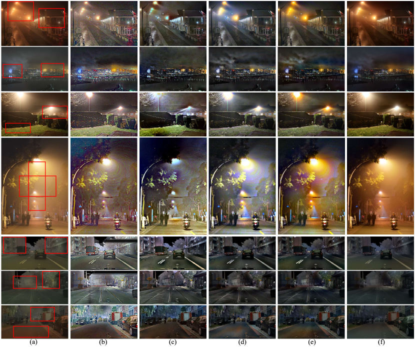
Figure 6. (a) Nighttime hazy images. (b) NDIM (Zhang et al., 2014). (c) GS (Li et al., 2015). (d) MRP (Zhang et al., 2017). (e) Our OSFD. (f) Our ND-Net.

6.3. Running time comparison

We evaluated the run-time of the different methods (Zhang et al., 2014; Li et al., 2015; Zhang et al., 2017) on a PC with an Intel CORE i7 CPU and 16 Gb memory and ND-Net on a Tesla V100 GPU. The codes are from the original authors. NDIM (Zhang et al., 2014), GS (Li et al., 2015), MRPF (Zhang et al., 2017), MRP (Zhang et al., 2017), our OSFD and ND-Net process a 512x512 image in 5.63s, 22.52s, 0.236s, 1.769s, 0.576s, and 0.0074s, respectively. Although OSFD calculates $\bm{{\rm{\eta}}}$ at 10 scales, it is 3x faster than MRP and 10x faster than NDIM and GS. The efficiency of OSFD arises from its $\mathcal{O}\left(\left|\mathcal{S}\right|N\right)$ complexity and the acceleration tricks used in Section 4.3. Since the basic operations in OSFD are paralleled, it promises to be faster using GPU acceleration. The proposed ND-Net is the fastest one and runs at 135 frames per second (FPS), benefiting from its lightweight backbone and GPU acceleration. It is promising to be used for real-time applications.

6.4. Limitations and discussion

Although the synthetic nighttime hazy images produced by 3R are visually realistic, they may contain artifacts due to inaccurate depth, i.e., the car boundaries in Figure 3. This can be addressed by using effective depth filtering/completion methods. Further, the light sources are set to isotropic point lights, which can be changed to other forms of light sources, $e.g.$, directional light, and volume light. Also, we can further add the glow images of virtual light sources into the final hazy image according to Eq. (3) in (Li et al., 2015) to simulate the glow effect. OSFD may generate results with color artifacts and residual haze due to the following limitations. 1) The statistical prior may not work in large monochromatic areas or dense haze regions with different color casts. 2) The optimal scale may be inaccurate if the initial dehazing stage fails. 3) Since dehazing is disentangled from color cast removal, it may be affected by the residual color cast. For example, see the trees and light sources in the first and fourth rows and the bluish distant areas in the last row in Figure 6.

Encouraged by recent progress in daytime dehazing, we are optimistic that deep models have the potential to address these limitations as evidenced by the proposed simple baseline ND-Net. There is still a large room for future studies. 3R generates a large amount of visually realistic training images with intermediate ground truth labels including low-light images, color cast, and illuminance, which can provide auxiliary supervision to train a better model. For example, devising disentangled generative models based on the explicit imaging model and intermediate labels is also very promising.

7. Conclusion

We introduce a novel synthetic method called 3R, which leverages both scene geometry and real-world light colors to generate realistic nighttime hazy images. Based on 3R, we construct a new dataset to benchmark state-of-the-art nighttime dehazing methods concerning haze removal, color cast correction, and runtime. We also propose an optimal-scale maximum reflectance prior, which can adapt to the local statistics at varying scales in natural images. Based on this, we disentangle the color correction from haze removal and devise a computationally efficient and effective dehazing method. Besides, we devise a simple but effective CNN-based baseline model, which shows good dehazing and generalization ability. Extensive experiments demonstrate their superiority over SOTA methods in terms of both image quality and runtime.

8. Nighttime Dehazing with a Synthetic Benchmark: Supplementary Material

8.1. More synthetic results generated by the proposed 3R

In this part, we present more visual results synthesized by the proposed 3R (see Section 3 in the paper for more details.). First, we compare the proposed 3R with the synthetic method in (Zhang et al., 2017) in Section 8.1.1. Then, we present some controllable synthetic results by changing the hyper-parameters in 3R, $e.g.$, $\beta_{t}$ for haze density, $\eta$ for light colors, and $\beta_{l}$ for illuminance intensity in Section 8.1.2. Finally, we also present some synthetic results on the Virtual KITTI dataset (Gaidon et al., 2016) in Section 8.1.3.

8.1.1. Visual comparison with the synthetic method in (Zhang et al., 2017)

Figure 7 and 8 show the synthetic nighttime hazy images generated by the proposed 3R and the method in (Zhang et al., 2017). As can be seen, the overall light colors are uniform, $i.e.$, yellow, in Figure 7(c) and 8(c). By contrast, the light colors in our 3R’s results are more realistic, $i.e.$, changed from light yellow to warm red. Meanwhile, the color cast at different areas within an image may be different since we randomly sampled light colors from the prior distribution (see Section 3.1 in the paper). Consequently, it is more challenging to deal with the non-uniform color cast.

Further, the results generated by (Zhang et al., 2017) have a strong vignetting effect since the method renders the illuminance from a single central light source and the illuminance intensity is only determined by the light path distance. By contrast, on the one hand, we consider the scene geometry when calculating the illuminance, $i.e.$, the illuminance intensity is calculated from the surface normal vector, the incident light direction, and the light path distance according to Lambert’s cosine law (Basri and Jacobs, 2003) (see Section 3.2 in the paper for more details.). On the other hand, we place many virtual light sources along the roadsides, which are 5 meters high and spaced every 30 meters. Consequently, the synthetic illuminance by 3R looks more realistic.

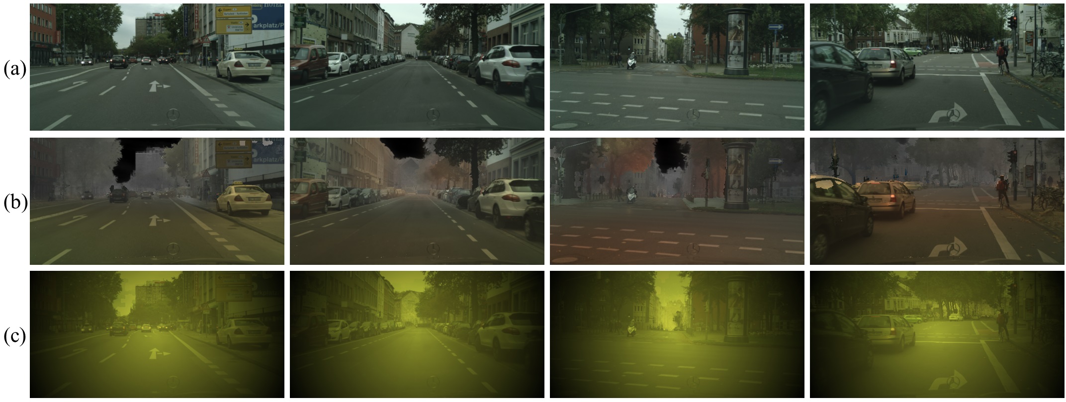
Figure 7. (a) Daytime clear images from the Cityscapes dataset (Cordts et al., 2016). (b) Synthetic results generated by the proposed 3R (see Section 3 in the paper. (c) Results generated by the method in (Zhang et al., 2017).

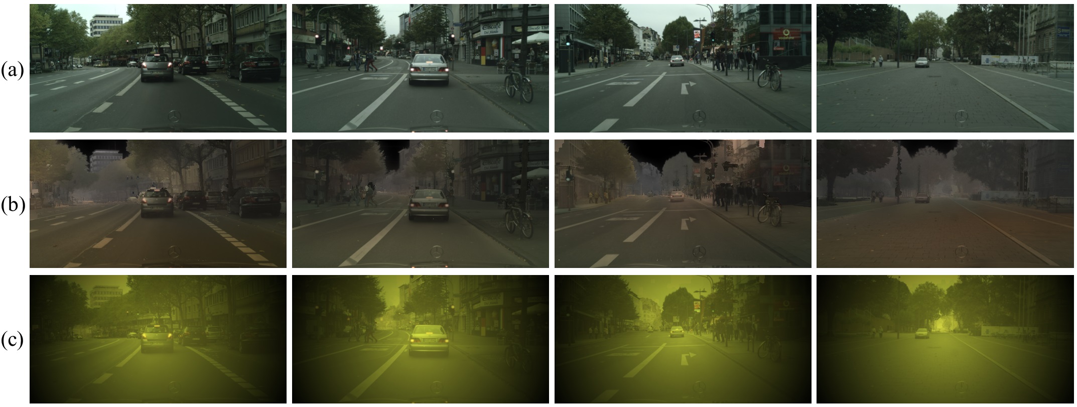
Figure 8. (a) Daytime clear images from the Cityscapes dataset (Cordts et al., 2016). (b) Synthetic results generated by the proposed 3R (see Section 3 in the paper.). (c) Results generated by the method in (Zhang et al., 2017).

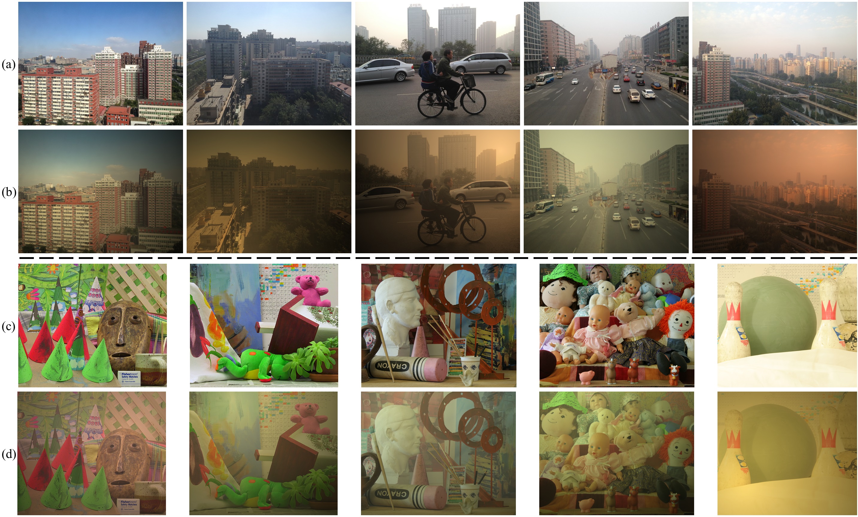
Figure 9. (a) Daytime clear images from the RESIDE dataset (Li et al., 2018). (b) The synthetic nighttime hazy images generated by the method in (Zhang et al., 2017). The light colors are sampled from the priori distribution in Section 3.1. (c) Daytime clear images from the Middlebury dataset (Scharstein and Szeliski, 2003). (d) The synthetic nighttime hazy images generated by the method in (Zhang et al., 2017). The light colors are sampled from the priori distribution in Section 3.1.

In (Zhang et al., 2017), they synthesized the nighttime hazy images on the Middlebury dataset (Scharstein and Szeliski, 2003). However, it is not trivial to use 3R on this dataset since the images are all captured in an indoor environment and there are no semantic labels available. Alternatively, we followed (Zhang et al., 2017) but replaced the constant yellow light color with the randomly sampled real-world light colors described in Section 3.1. Similarly, we also synthesized nighttime hazy images on the RESIDE dataset (Li et al., 2018). The results in Figure 9 (b) and (d) show more diversity in illuminance colors than Figure 7(c) and Figure 8(c). These two synthetic datasets are denoted NHM and NHR, respectively.

Some visual results using different methods on NHM and NHR are presented in Figure 10. Since images in NHM have a shallow depth of field (DOF) in the indoor environment and colorful objects, the methods (Zhang et al., 2014; Li et al., 2015; Zhang et al., 2017) and our OSFD tend to generate over-dehazed results, resulting in more saturated colors (see the white plaster and the canvas in the first two rows in Figure 10). Nevertheless, the proposed OSFD achieves better results than others. For example, MRP (Zhang et al., 2017) generates whitish results with color artifacts (see the areas enclosed by the red rectangles.). On the NHR dataset, our OSFD can efficiently remove the haze while retaining the colors as shown in the last two rows in Figure 10. Generally, the proposed ND-Net achieves the best performance on both NHM and NHR datasets, which efficiently correct the color cast and remove haze.

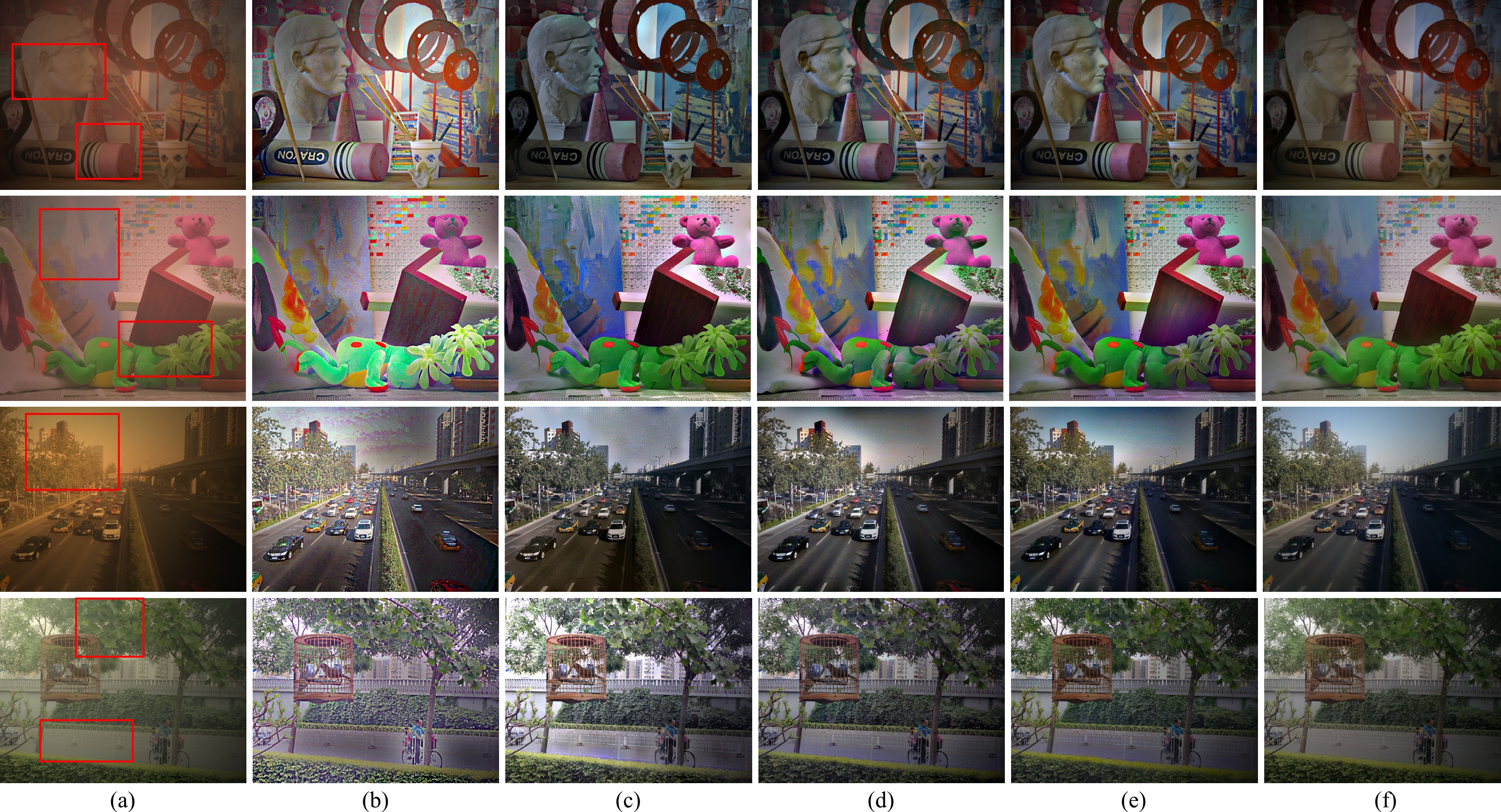
Figure 10. (a) Nighttime hazy images from NHM and NHR datasets. (b) NDIM (Zhang et al., 2014). (c) GS (Li et al., 2015). (d) MRP (Zhang et al., 2017). (e) Our OSFD (see Section 4.2 in the paper). (f) Our ND-Net (see Section 5 in the paper).

8.1.2. Controllable synthetic results generated by 3R

In our 3R method, some hyper-parameters such as $\beta_{t}$, $\eta$, $\beta_{l}$, can be changed to generate controllable synthetic nighttime hazy images, for example, light haze or dense haze, low illuminance or high illuminance. It could be very useful for training deep neural networks with better generalizability and disentangling the degradation factors in nighttime (hazy) images.

Haze Density As shown in Figure 11, with the increasing of $\beta_{t}$ from 0.005 to 0.025, the transmission maps (Figure 11(a)) become darker, and the hazy images (Figure 11(b) and (c)) contain more and more haze. It is noteworthy that we kept the illuminance intensity and light colors (Figure 11(d)) fixed in this experiment.

Light Colors As shown in Figure 12, we sampled different light colors from the prior distribution (see Section 3.1 in the paper.), resulting in diverse color casts (Figure 12(a)). Accordingly, the synthetic nighttime (hazy) images have more diversity in light colors (Figure 12(b) and (c)). We kept the illuminance intensity and transmission fixed in this experiment.

Illuminance Intensity As shown in Figure 13, with the increasing of $\beta_{l}$ from 0.02 to 1, the illuminance intensity becomes lower (Figure 13(a)), and the nighttime (hazy) images (Figure 11(b)$\sim$(d)) become darker accordingly. We kept the light colors and haze transmission (Figure 13(e)) fixed in this experiment.

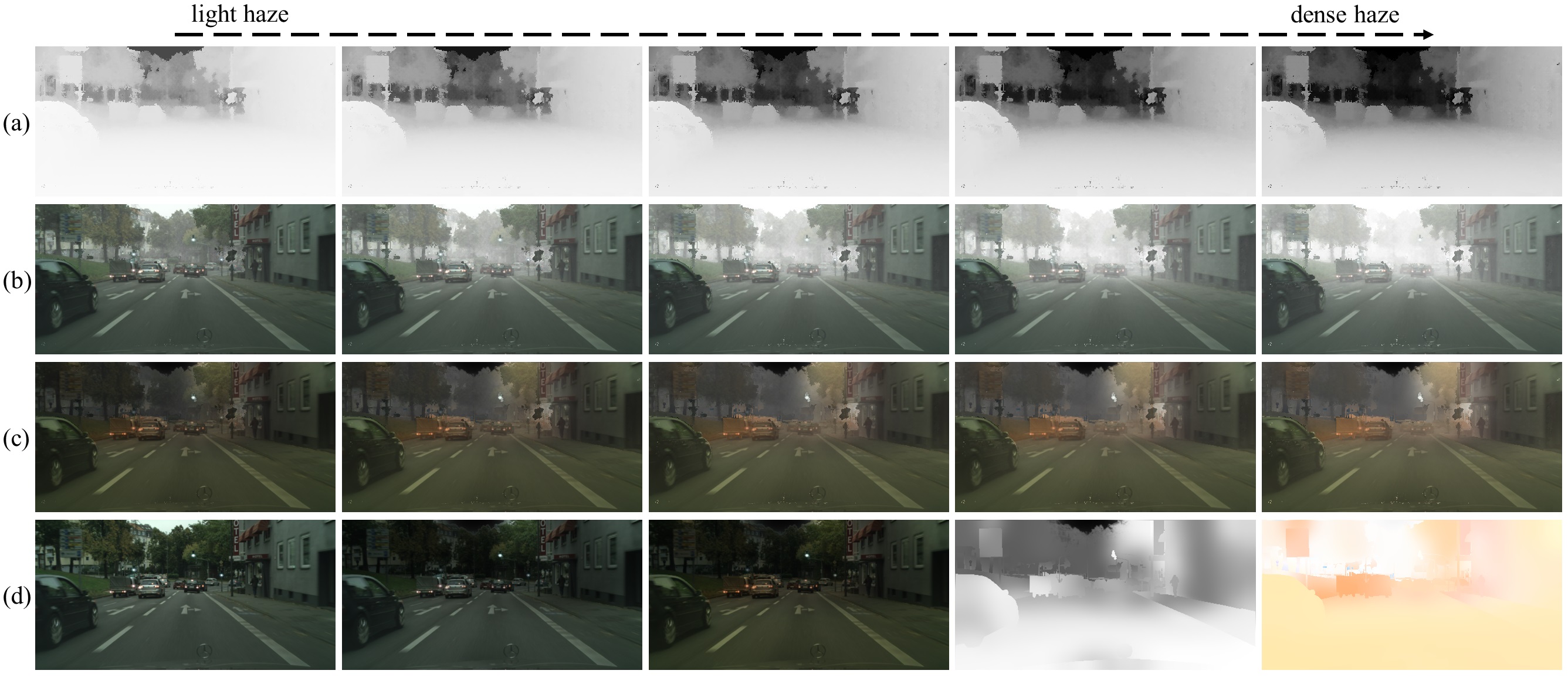
Figure 11. (a) The transmission maps at different haze density levels, $i.e.$, $\beta_{t}=0.005,0.01,...,0.025$. (b) The synthetic daytime hazy images generated by 3R. (c) The synthetic nighttime hazy images generated by 3R. (d) From left to right, the original daytime clear image, the synthetic nighttime images without/with color cast, the illuminance intensity map, and the color cast map.

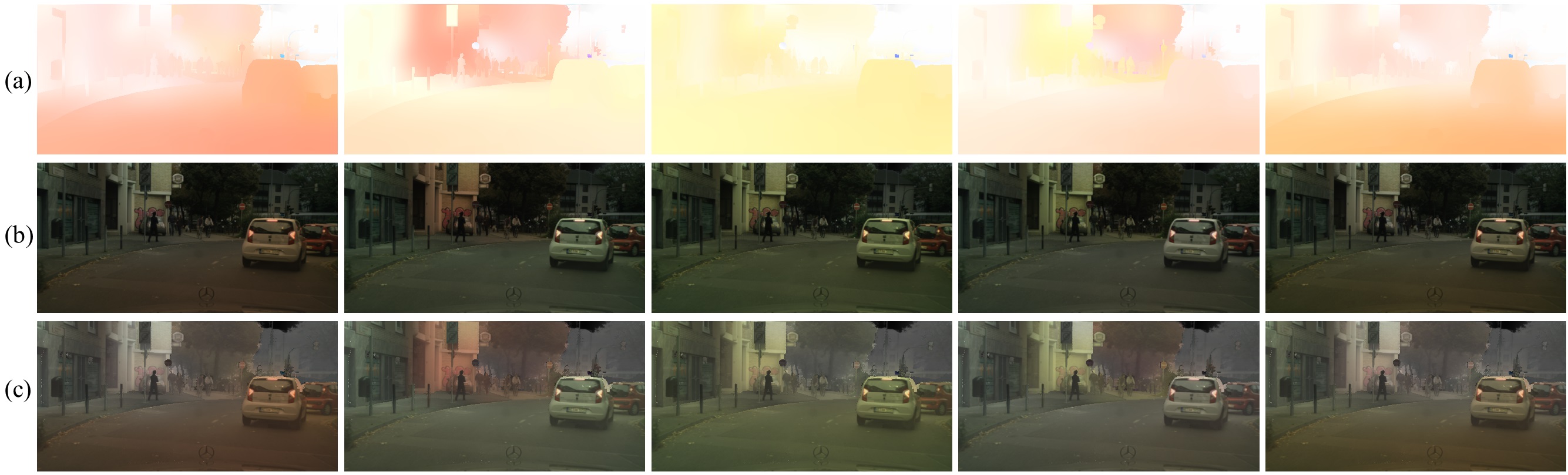
Figure 12. (a) Color cast maps by randomly sampling light colors (see Section 3.1 in the paper.). (b) The synthetic nighttime images with color cast generated by 3R. (c) The synthetic nighttime hazy images generated by 3R.

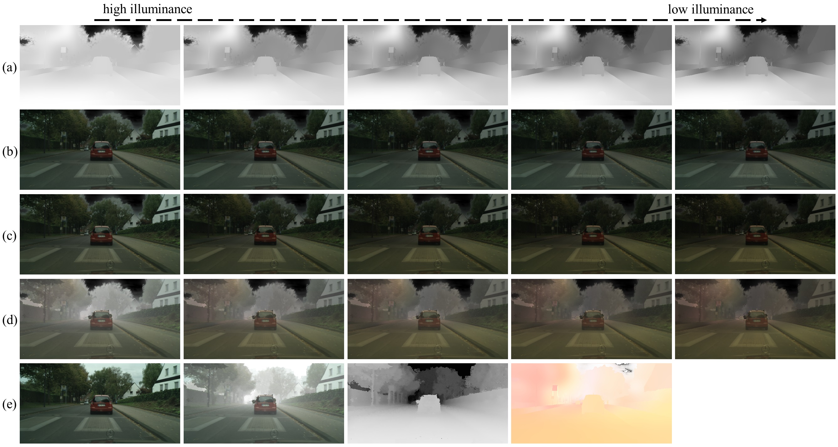
Figure 13. (a) The illuminance maps at different illumination levels, $i.e.$, $\beta_{l}=0.02,0.04,...,1$ (see Section 3.2 in the paper.). (b) The synthetic nighttime images without color cast generated by 3R. (c) The synthetic nighttime images with color cast generated by 3R. (d) The synthetic nighttime hazy images generated by 3R. (e) From left to right, the original daytime clear image, the daytime hazy image, the transmission map, and the color cast map.

8.1.3. Visual results on Virtual KITTI generated by 3R

Our 3R method can also generate nighttime hazy images based on the Virtual KITTI dataset (Gaidon et al., 2016). It is noteworthy that nighttime hazy imaging condition is not available in the dataset. Some results are shown in Figure 14, which look reasonable. Considering that the original images in the Virtual KITTI dataset are rendered by a 3D game engine where the textures are not so realistic, we do not include them in our benchmark. In the future, we can try to synthesize images on the original KITTI images (Geiger et al., 2012) by estimating the absent depth maps or semantic labels.

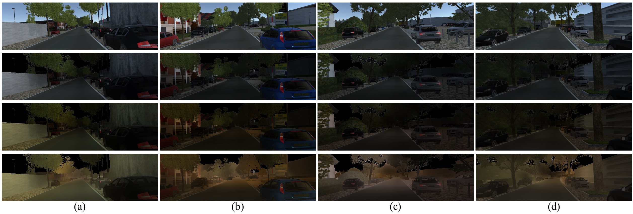
Figure 14. (a) Daytime clear images from the Virtual KITTI dataset (Gaidon et al., 2016). (b) The synthetic nighttime images without color cast generated by 3R. (c) The synthetic nighttime images with color cast generated by 3R. (d) The synthetic nighttime hazy images generated by 3R.

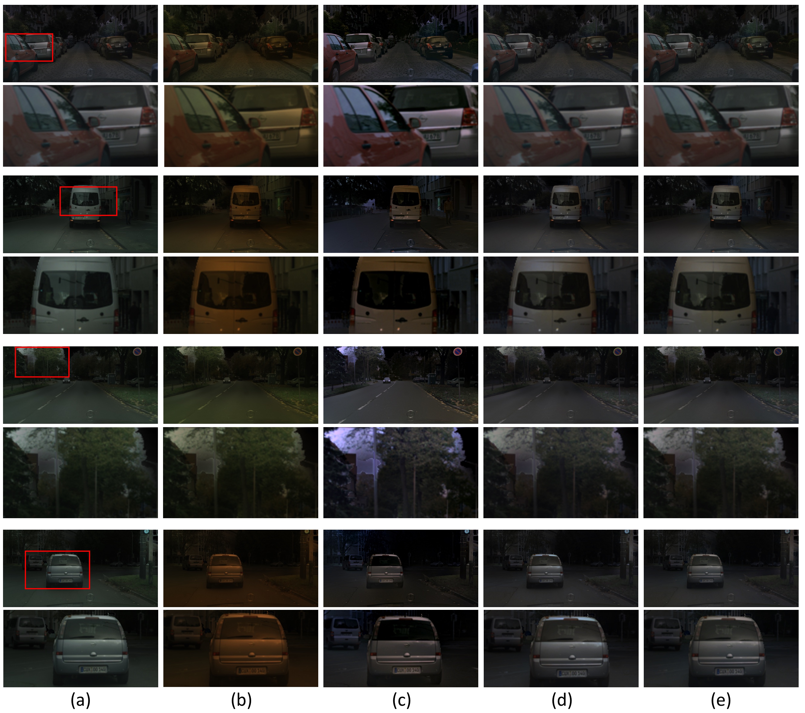
Figure 15. (a)-(b) The synthetic nighttime images without/with color cast generated by 3R. (c) GS (Li et al., 2015). (d) MRP (Zhang et al., 2017). (e) Our OSFD. The even rows show the close-up views of the red rectangles.

8.2. Comparison with state-of-the-art dehazing methods

8.2.1. Visual comparison for color cast removal

We also conducted an experiment to compare different methods for color cast removal as described in Section 5.2 and Table 4 in the paper. In this part, we present some visual results in Figure 15 and 16. Since OSFD adaptively chooses the best scale to estimate the color cast, it can handle the monochromatic areas such as cars and trees in Figure 15, and avoid the whitish effect or residual color cast in MRP’s results (Zhang et al., 2017). The results on the daytime clear images without color cast also demonstrate the superiority of OSFD for retaining intrinsic image colors.

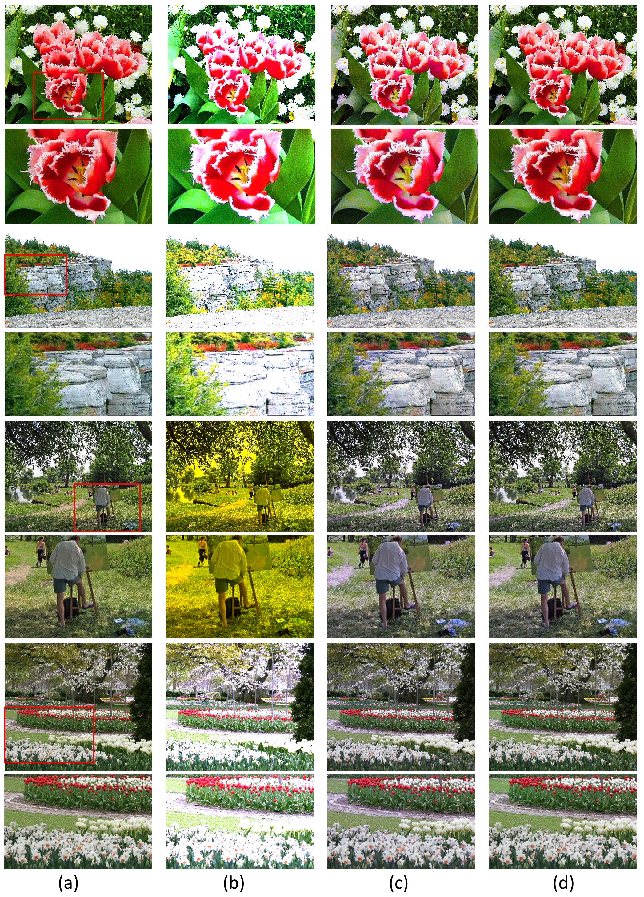
Figure 16. (a) The daytime clear images from the DCRW dataset (see Section 3.3). (b) GS (Li et al., 2015). (c) MRP (Zhang et al., 2017). (d) Our OSFD. The even rows show the close-up views of the red rectangles.

8.3. Hyper-parameter settings

8.3.1. Hyper-parameter settings for ND-Net

In this part, we present the brief ablation studies on the proposed ND-Net including training epochs, input image size, batch size, and losses. The results are summarized in Table 5. As can be seen, using a large input image size, training for a long time, as well as employing the perceptual loss can improve the dehazing results. We choose the setting listed in the last row as the default one in the paper.

Table 5. Hyper-parameter setting studies on the NHR dataset. E: training epochs; B: batch Size; S: input image size; MSE: MSE loss; MSE+PL: MSE and Perceptual loss

Method	PSNR ($\uparrow$)	SSIM ($\uparrow$)	CIEDE2000 ($\downarrow$)
E=70, B=8, S=128, MSE	26.54	0.9286	5.82
E=70, B=8, S=256, MSE	27.18	0.9312	5.05
E=300, B=8, S=256, MSE	28.95	0.9413	4.30
E=300, B=8, S=256, MSE+PL	28.74	0.9465	4.02

8.3.2. The number of scales in OSFD

We conducted a parameter study on the number of scales used in OSFD. The results are reported on the NHC-L dataset as shown in Figure 17. Using more scales, OSFD achieves lower CIEDE2000 scores, implying better color cast removal results. There is a steep drop at the beginning (1$\sim$5 scales), and then the performance saturates. Considering that OSFD is computationally efficient and the color artifacts in the dehazed results are annoying, we choose 10 scales for OSFD in other experiments to obtain better visual results.

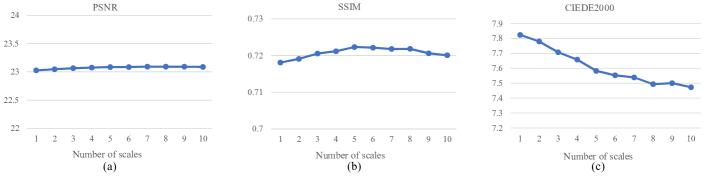
Figure 17. Results of OSFD using different number of scales on the NHC-L dataset. (a) PSRN. (b) SSIM. (c) CIEDE2000.

Table 6. Standard deviations of the dehazing results on the NHC dataset.

	NHC-L			NHC-M			NHC-D
Method	PSNR ($\uparrow$)	SSIM ($\uparrow$)	CIEDE2000 ($\downarrow$)	PSNR ($\uparrow$)	SSIM ($\uparrow$)	CIEDE2000 ($\downarrow$)	PSNR ($\uparrow$)	SSIM ($\uparrow$)	CIEDE2000 ($\downarrow$)
NDIM (Zhang et al., 2014)	0.0113	0.0010	0.0363	0.0136	0.0019	0.0524	0.0059	0.0013	0.0123
GS (Li et al., 2015)	0.0172	0.0015	0.0268	0.0228	0.0014	0.0247	0.0146	0.0011	0.0309
MRPF (Zhang et al., 2017)	0.0144	0.0007	0.0131	0.0131	0.0006	0.0139	0.0051	0.0007	0.0151
MRP (Zhang et al., 2017)	0.0031	0.0004	0.0091	0.0071	0.0005	0.0194	0.0024	0.0009	0.0174
OSFD	0.0072	0.0006	0.0134	0.0085	0.0008	0.0178	0.0016	0.0010	0.0196

Since we augmented the Cityscapes by 5 times when generating the NHC dataset (see Section 3.3), the results listed in Table 2 in the paper are obtained by averaging the scores from all five tests. The corresponding standard deviations are listed in Table 6. As can be seen, the standard deviations are very low. Since we carried out each evaluation on all the 550 images, the score from each evaluation is stable even if we changed the light colors randomly during each augmentation.

References

- (1)
- Achanta et al. (2012) Radhakrishna Achanta, Appu Shaji, Kevin Smith, Aurelien Lucchi, Pascal Fua, and Sabine Süsstrunk. 2012. SLIC superpixels compared to state-of-the-art superpixel methods. IEEE transactions on pattern analysis and machine intelligence 34, 11 (2012), 2274–2282.
- Ancuti et al. (2016) Cosmin Ancuti, Codruta O Ancuti, Christophe De Vleeschouwer, and Alan C Bovik. 2016. Night-time dehazing by fusion. In 2016 IEEE International Conference on Image Processing (ICIP). IEEE, 2256–2260.
- Ancuti et al. (2018a) Cosmin Ancuti, Codruta O Ancuti, Radu Timofte, and Christophe De Vleeschouwer. 2018a. I-HAZE: a dehazing benchmark with real hazy and haze-free indoor images. In International Conference on Advanced Concepts for Intelligent Vision Systems. Springer, 620–631.
- Ancuti et al. (2018b) Codruta O. Ancuti, Cosmin Ancuti, Radu Timofte, and Christophe De Vleeschouwer. 2018b. O-HAZE: A Dehazing Benchmark With Real Hazy and Haze-Free Outdoor Images. In The IEEE Conference on Computer Vision and Pattern Recognition (CVPR) Workshops.
- Barron (2015) Jonathan T Barron. 2015. Convolutional color constancy. In Proceedings of the IEEE International Conference on Computer Vision. 379–387.
- Barron and Tsai (2017) Jonathan T Barron and Yun-Ta Tsai. 2017. Fast fourier color constancy. In Proceedings of the IEEE Conference on Computer Vision and Pattern Recognition. 886–894.
- Basri and Jacobs (2003) Ronen Basri and David W Jacobs. 2003. Lambertian reflectance and linear subspaces. IEEE Transactions on Pattern Analysis & Machine Intelligence 2 (2003), 218–233.
- Berman et al. (2016) Dana Berman, Shai Avidan, et al. 2016. Non-local image dehazing. In Proceedings of the IEEE conference on computer vision and pattern recognition. 1674–1682.
- Buchsbaum (1980) Gershon Buchsbaum. 1980. A spatial processor model for object colour perception. Journal of the Franklin institute 310, 1 (1980), 1–26.
- Cai et al. (2016) Bolun Cai, Xiangmin Xu, Kui Jia, Chunmei Qing, and Dacheng Tao. 2016. Dehazenet: An end-to-end system for single image haze removal. IEEE Transactions on Image Processing 25, 11 (2016), 5187–5198.
- Cordts et al. (2016) Marius Cordts, Mohamed Omran, Sebastian Ramos, Timo Rehfeld, Markus Enzweiler, Rodrigo Benenson, Uwe Franke, Stefan Roth, and Bernt Schiele. 2016. The cityscapes dataset for semantic urban scene understanding. In Proceedings of the IEEE conference on computer vision and pattern recognition. 3213–3223.
- Deng et al. (2019) Zijun Deng, Lei Zhu, Xiaowei Hu, Chi-Wing Fu, Xuemiao Xu, Qing Zhang, Jing Qin, and Pheng-Ann Heng. 2019. Deep Multi-Model Fusion for Single-Image Dehazing. In The IEEE International Conference on Computer Vision (ICCV).
- Fattal (2014) Raanan Fattal. 2014. Dehazing using color-lines. ACM transactions on graphics (TOG) 34, 1 (2014), 13.
- Gaidon et al. (2016) Adrien Gaidon, Qiao Wang, Yohann Cabon, and Eleonora Vig. 2016. Virtual worlds as proxy for multi-object tracking analysis. In Proceedings of the IEEE conference on computer vision and pattern recognition. 4340–4349.
- Geiger et al. (2012) Andreas Geiger, Philip Lenz, and Raquel Urtasun. 2012. Are we ready for autonomous driving? the kitti vision benchmark suite. In 2012 IEEE Conference on Computer Vision and Pattern Recognition. IEEE, 3354–3361.
- He and Sun (2015) Kaiming He and Jian Sun. 2015. Fast guided filter. arXiv preprint arXiv:1505.00996 (2015).
- He et al. (2009) Kaiming He, Jian Sun, and Xiaoou Tang. 2009. Single image haze removal using dark channel prior. In 2009 IEEE Conference on Computer Vision and Pattern Recognition. IEEE, 1956–1963.
- He et al. (2010) Kaiming He, Jian Sun, and Xiaoou Tang. 2010. Guided image filtering. In European conference on computer vision. Springer, 1–14.
- Hu et al. (2017) Yuanming Hu, Baoyuan Wang, and Stephen Lin. 2017. Fc4: Fully convolutional color constancy with confidence-weighted pooling. In Proceedings of the IEEE Conference on Computer Vision and Pattern Recognition. 4085–4094.
- Johnson et al. (2016) Justin Johnson, Alexandre Alahi, and Li Fei-Fei. 2016. Perceptual losses for real-time style transfer and super-resolution. In European conference on computer vision. Springer, 694–711.
- Joze et al. (2012) Hamid Reza Vaezi Joze, Mark S Drew, Graham D Finlayson, and Perla Aurora Troncoso Rey. 2012. The role of bright pixels in illumination estimation. In Color and Imaging Conference, Vol. 2012. Society for Imaging Science and Technology, 41–46.
- Li et al. (2017) Boyi Li, Xiulian Peng, Zhangyang Wang, Jizheng Xu, and Dan Feng. 2017. Aod-net: All-in-one dehazing network. In Proceedings of the IEEE International Conference on Computer Vision. 4770–4778.
- Li et al. (2018) Boyi Li, Wenqi Ren, Dengpan Fu, Dacheng Tao, Dan Feng, Wenjun Zeng, and Zhangyang Wang. 2018. Benchmarking single-image dehazing and beyond. IEEE Transactions on Image Processing 28, 1 (2018), 492–505.
- Li et al. (2019) Yunan Li, Qiguang Miao, Wanli Ouyang, Zhenxin Ma, Huijuan Fang, Chao Dong, and Yining Quan. 2019. LAP-Net: Level-Aware Progressive Network for Image Dehazing. In The IEEE International Conference on Computer Vision (ICCV).
- Li et al. (2015) Yu Li, Robby T Tan, and Michael S Brown. 2015. Nighttime haze removal with glow and multiple light colors. In Proceedings of the IEEE International Conference on Computer Vision. 226–234.
- Liu et al. (2019) Xiaohong Liu, Yongrui Ma, Zhihao Shi, and Jun Chen. 2019. GridDehazeNet: Attention-Based Multi-Scale Network for Image Dehazing. In Proceedings of the IEEE International Conference on Computer Vision. 7314–7323.
- Millerson (2013) Gerald Millerson. 2013. Lighting for TV and Film. Routledge. 26 pages.
- Pei and Lee (2012) Soo-Chang Pei and Tzu-Yen Lee. 2012. Nighttime haze removal using color transfer pre-processing and dark channel prior. In 2012 19th IEEE International Conference on Image Processing. IEEE, 957–960.
- Ren et al. (2016) Wenqi Ren, Si Liu, Hua Zhang, Jinshan Pan, Xiaochun Cao, and Ming-Hsuan Yang. 2016. Single image dehazing via multi-scale convolutional neural networks. In European conference on computer vision. Springer, 154–169.
- Ren et al. (2018) Wenqi Ren, Lin Ma, Jiawei Zhang, Jinshan Pan, Xiaochun Cao, Wei Liu, and Ming-Hsuan Yang. 2018. Gated fusion network for single image dehazing. In Proceedings of the IEEE Conference on Computer Vision and Pattern Recognition. 3253–3261.
- Sakaridis et al. (2018) Christos Sakaridis, Dengxin Dai, and Luc Van Gool. 2018. Semantic foggy scene understanding with synthetic data. International Journal of Computer Vision 126, 9 (2018), 973–992.
- Scharstein and Szeliski (2003) Daniel Scharstein and Richard Szeliski. 2003. High-accuracy stereo depth maps using structured light. In 2003 IEEE Computer Society Conference on Computer Vision and Pattern Recognition, 2003. Proceedings., Vol. 1. IEEE, I–I.
- Sharma et al. (2005) Gaurav Sharma, Wencheng Wu, and Edul N Dalal. 2005. The CIEDE2000 color-difference formula: Implementation notes, supplementary test data, and mathematical observations. Color Research & Application 30, 1 (2005), 21–30.
- Simonyan and Zisserman (2015) Karen Simonyan and Andrew Zisserman. 2015. Very Deep Convolutional Networks for Large-Scale Image Recognition. In International Conference on Learning Representations (ICLR 2015).
- Tang et al. (2014) Ketan Tang, Jianchao Yang, and Jue Wang. 2014. Investigating haze-relevant features in a learning framework for image dehazing. In Proceedings of the IEEE conference on computer vision and pattern recognition. 2995–3000.
- Van De Weijer et al. (2007) Joost Van De Weijer, Theo Gevers, and Arjan Gijsenij. 2007. Edge-based color constancy. IEEE Transactions on image processing 16, 9 (2007), 2207–2214.
- Wang et al. (2020) Yang Wang, Yang Cao, Zheng-Jun Zha, Jing Zhang, and Zhiwei Xiong. 2020. Deep Degradation Prior for Low-Quality Image Classification. In Proceedings of the IEEE/CVF Conference on Computer Vision and Pattern Recognition (CVPR).
- Wang et al. (2004) Zhou Wang, Alan C Bovik, Hamid R Sheikh, Eero P Simoncelli, et al. 2004. Image quality assessment: from error visibility to structural similarity. IEEE transactions on image processing 13, 4 (2004), 600–612.
- Yang and Sun (2018) Dong Yang and Jian Sun. 2018. Proximal dehaze-net: a prior learning-based deep network for single image dehazing. In Proceedings of the European Conference on Computer Vision (ECCV). 702–717.
- Zhang and Patel (2018) He Zhang and Vishal M Patel. 2018. Densely connected pyramid dehazing network. In Proceedings of the IEEE conference on computer vision and pattern recognition. 3194–3203.
- Zhang et al. (2017) Jing Zhang, Yang Cao, Shuai Fang, Yu Kang, and Chang Wen Chen. 2017. Fast haze removal for nighttime image using maximum reflectance prior. In Proceedings of the IEEE Conference on Computer Vision and Pattern Recognition. 7418–7426.
- Zhang et al. (2018) Jing Zhang, Yang Cao, Yang Wang, Chenglin Wen, and Chang Wen Chen. 2018. Fully Point-wise Convolutional Neural Network for Modeling Statistical Regularities in Natural Images. In ACM Multimedia Conference.
- Zhang et al. (2014) Jing Zhang, Yang Cao, and Zengfu Wang. 2014. Nighttime haze removal based on a new imaging model. In 2014 IEEE International Conference on Image Processing (ICIP). IEEE, 4557–4561.
- Zhang and Tao (2020) Jing Zhang and Dacheng Tao. 2020. FAMED-Net: A Fast and Accurate Multi-scale End-to-end Dehazing Network. IEEE Transactions on Image Processing 29 (2020), 72–84. https://doi.org/10.1109/TIP.2019.2922837
- Zhu et al. (2015) Qingsong Zhu, Jiaming Mai, and Ling Shao. 2015. A fast single image haze removal algorithm using color attenuation prior. IEEE transactions on image processing 24, 11 (2015), 3522–3533.