Aggregating Quantum Networks

Abstract

Quantum networking allows the transmission of information in ways unavailable in the classical world. Single packets of information can now be split and transmitted in a coherent way over different routes. This aggregation allows information to be transmitted in a fault tolerant way between different parts of the quantum network (or the future internet) – even when that is not achievable with a single path approach. It is a quantum phenomenon not available in conventional telecommunication networks either. We show how the multiplexing of independent quantum channels allows a distributed form of quantum error correction to protect the transmission of quantum information between nodes or users of a quantum network. Combined with spatial-temporal single photon multiplexing we observe a significant drop in network resources required to transmit that quantum signal – even when only two channels are involved. This work goes far beyond the concepts of channel capacities and shows how quantum networking may operate in the future. Further it shows that quantum networks are likely to operate differently from their classical counterparts which is an important distinction as we design larger scale ones.

I Introduction

Our recent advances have brought quantum technologies from an abstract thought experiment to reality with many pivotal demonstrations being achieved and even devices available for commercial use Higginbotham et al. (2018); Kelly (2018); Karalic et al. (2020); Feng et al. (2020); Caneva et al. (2020); Christensen et al. (2020); Anderson et al. (2019). Such technologies can be characterized into a number of broad areas including quantum computation Nielsen and Chuang (2000); Bennett and DiVincenzo (2000); Raussendorf and Briegel (2001); Knill (2005); Duan and Raussendorf (2005), communication Bennett and Brassard (2014); Munro et al. (2015); Sangouard et al. (2011); Duan et al. (2001); Lo (1999); Hwang (2003); Ekert (1991); Qiu (2014); Bunandar et al. (2018), metrology Toth (2012); Guo-Yong and Guang-Can (2013), sensing and imaging Dogen et al. (2017); Lugiato et al. (2002); Simon et al. (2014). We have achieved remarkable control over these systems and recently a “quantum advantage” has been achieved in the quantum computational regime on a monolithic chip Arute et al. (2019). Quantum communication also holds significant promise – but clearly is not as advanced yet. We have however seen quantum key distribution networks operating on a continental scale Qiu (2014); Liao et al. (2017) but this is far from a future multi-purpose global quantum internet Kimble (2008).

In any future quantum internet, we are going to need to be able to send (or transmit) quantum information over large distances – potentially through many intermediate routing nodes. Whether this occurs by the direct transmission of such information Bunandar et al. (2018); Munro et al. (2012) or by quantum teleportation Bennett et al. (1996); Deng et al. (2005); Barrett et al. (2004); Ma et al. (2012) after an entangled resource has been established Huang et al. (2020) we already know that some mechanism to handle both loss and local gate errors will be necessary Nielsen and Chuang (2000). Approaches based on quantum error detection codes Deutsch et al. (1996); Dur and Briegel (2003), while attractive in the short term, are performance limited due to their reliance on probabilistic operations Deutsch et al. (1996); Munro et al. (2012, 2010). Scheme using quantum error correction for both loss and gate errors overcome such issues but are technically much more challenging Ralph et al. (2005); Grassl et al. (1999); Fowler et al. (2010); Gottesman et al. (2001); Munro et al. (2012); Jiang et al. (2009); Cochrane et al. (1999); Michael et al. (2016). Still for large scale quantum networks, they are likely to be the only viable approach.

We can picture a general quantum network as a complex network involving certain nodes connected to each other by quantum links. Within these nodes we have a certain number of quantum bits associated with those links to the adjacent node. In any multiuser scenario we are likely to be in a constrained resource situation and there may not be enough resources associated with one path to that adjacent nodes at that time to allow the reliable transmission of one’s error correction encoded signal. However, in these complex networks there are likely to be multiple paths between nodes (some potentially with immediate nodes in between). The natural question that arises is: if no path has sufficient resources by itself (either the number of qubits with the node or the capacity of the channel itself), can we combine (‘aggregate’) them together to achieve it? This will be the focus of our paper.

The concept of quantum network aggregation is of course not new having been considered by a number of groups in the context of establishing bounds of the quantum and private capacities Azuma and Kato (2017); Shirokov (2017); Rosati et al. (2018); Pirandola (2019a, b); Fanizza et al. (2020). Unfortunately, those capacities tell us limited information about what would have in a dynamical network where resources are being continuously utilized and potentially consumed, nor do they tell us how such aggregation can take place. In our work here we consider the simple situation of two resource constrained parties (Alice and Bob) who have two independent channels between themselves with different transmission properties. We show that single quantum states (packets) can be transmitted simultaneously over both channels in a coherent fashion – enabling its transmission which would not have been possible by either individual channel along. Further this adds a new capability to networking not present in the telecommunications world.

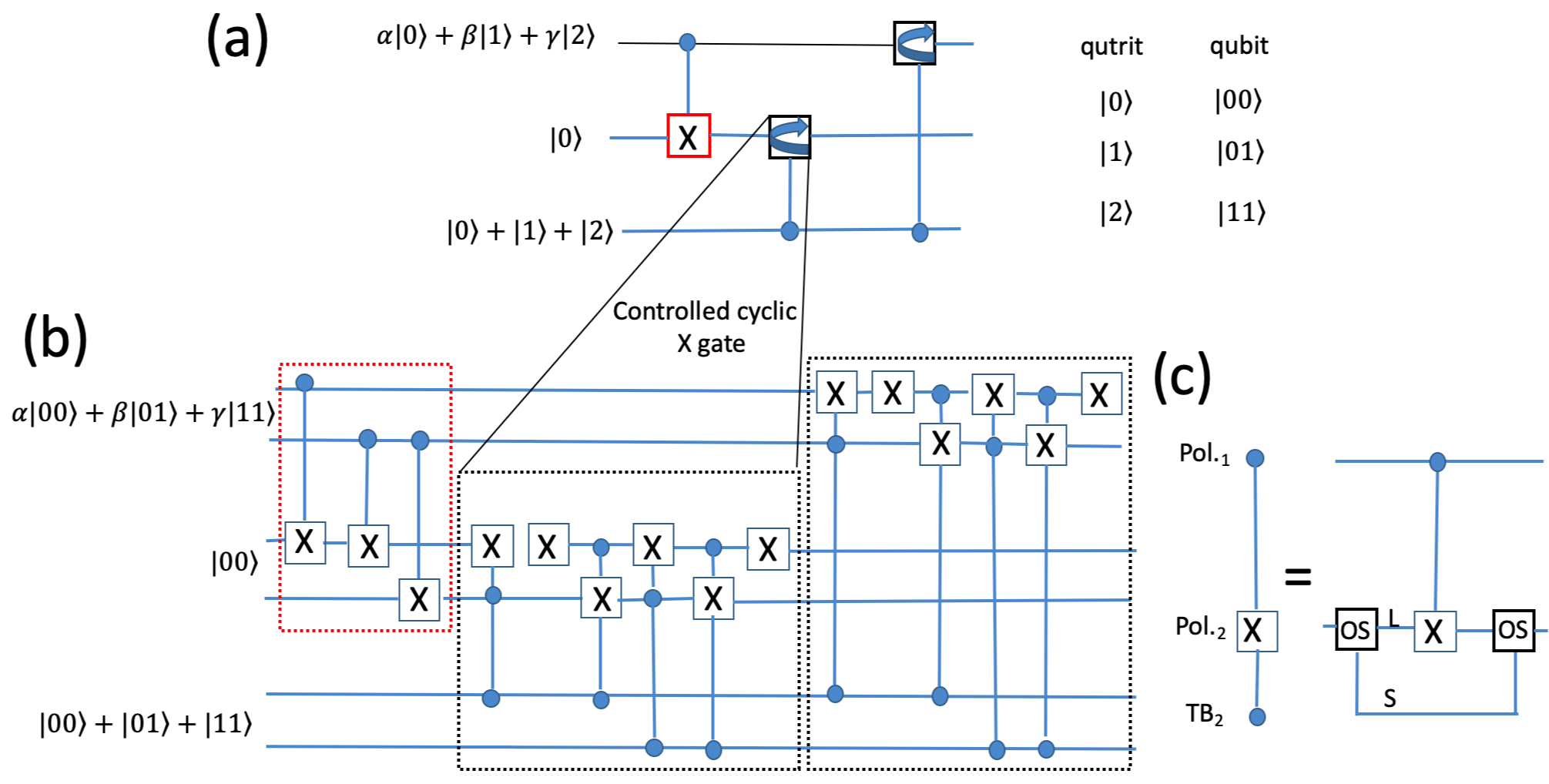
Figure 1: (a) Logic circuit used for the encoding of the (3,1,2) QRS code with qutrits, (b) gives the corresponding circuit using qubits while (c) illustrates how the Toffoli gate can be implemented for multiplexed photons using only a single photon-photon CNOT gate. This is potentially an important resource saving Ralph et al. (2007); Ioniciouiu et al. (2009). Here Pol.₁, Pol.₂ and TB₂ stand for the polarization DOFs of photon 1, photon 2 and time-bin DOF of photon 2 respectively. OS is an optical switch that splits into two other modes (Long and Short) photon 2. A CNOT between photon 1 and the Long component of photon 2 is performed followed by another OS that recombines the modes.

Recently, it been found that quantum multiplexing Lo Piparo et al. (2020) – the process whereby information is encoded into different degrees of freedom of a photon Kwiat (1997); Barreiro et al. (2005); Wei et al. (2007) – can dramatically decrease both the number of qubits required within the node and also the number of photons being transmitted through the channel (still this may not be enough). However, in conjunction with aggregation those advantages may be enhanced further.

The paper is divided as following: In Section II we briefly introduce communication-based quantum error correction in terms of the quantum Reed-Solomon (QRS) code and show how quantum multiplexing can be applied to it. Then in Section III we illustrate our aggregation scheme between two nodes with two different channels connecting them. This is followed up in Section IV with the extension to spatial-temporal single photon multiplexing. We conclude in Section V.

II The quantum Reed-Solomon code

It is well known that advanced quantum repeaters will be based on quantum error correction techniques Munro et al. (2012). There are a huge variety of codes available for use in these circumstances Ralph et al. (2005); Grassl et al. (1999); Fowler et al. (2010); Gottesman et al. (2001) but here our primary focus will be on the Quantum Reed Solomon (QRS) code Grassl et al. (1999). Such a code has excellent properties to handle channel loss events and has also recently been shown that the number of physical resources required to implement it can be dramatically reduced by using a quantum multiplexing approach Lo Piparo et al. (2020). The QRS code has been used in several applications in the last few years Grassl et al. (1999). In this Section we will review the QRS code and how it can be used in the quantum multiplexing regime.

The QRS code is typically written in the form $[[d,2k-d,d-k+1]]_{d}$, where $2k-d$ logic qudits of dimension $d$ (prime number) are encoded into $d$ physical qudits, in such a way that when $d-k$ or less qudits are lost the encoded qudit can be retrieved. A simple example of such a code is the $[[3,1,2]]_{3}$ code. Here a logic qutrit $\left.|D\right\rangle$ is encoded using three physical qutrits as Muralidharan et al. (2018):

$$\left.|D\right\rangle=\left.\alpha|0\right\rangle_{L}+\left.\beta|1\right\rangle_{L}+\left.\gamma|2\right\rangle_{L},$$ (1)

where (omitting the normalization constants for simplicity) $\left.|0\right\rangle_{L}=\left.|000\right\rangle+\left.|111\right\rangle+\left.|222\right\rangle,$ $\left.|1\right\rangle_{L}=\left.|012\right\rangle+\left.|120\right\rangle+\left.|201\right\rangle$ and $\left.|2\right\rangle_{L}=\left.|021\right\rangle+\left.|102\right\rangle+\left.|210\right\rangle$ (see Fig. 1(a) and Appendix A for further details). This code has used physical qutrits in its encoding, however it may be more convenient to use physical qubits due to their more common nature. As such we can use two qubits to encode one physical qutrit meaning six qubits are needed for the logical state to encode the $[[3,1,2]]_{3}$ code (see Fig. 1(b) and Appendix B). One can extend this encoding procedure to the multiplexed case Lo Piparo et al. (2020) in which each photon is carrying two qubits of information. This approach reduces number of physical resources in an error correction scheme Lo Piparo et al. (2020) (the usual Toffoli gate reduces to a simple CNOT gate as shown in Fig. 1(c)). Further details on how the logic qutrit $\left.|D\right\rangle$ can be created with the quantum multiplexing approach is shown in Appendix C.

In using these error correction techniques it is important to consider our figures of merit for how we assess the performance of those approaches. The main figure of merit we are interested in our analysis is the probability of successfully transmitting $d$ qudits over a lossy channel, $P_{S}(1\mathrm{ch)}$. For that generic $[[d,2k-d,d-k+1]]_{d}$ QRS code, in which photons are carrying $q$ qubits of information, any qudit depends on the successful transmission of $\lceil\log_{2}(d)/q\rceil$ photons Grassl et al. (1999). Therefore $P_{S}(1\mathrm{ch)}$ is given by Muralidharan et al. (2018):

$$P_{S}(1\mathrm{ch)}=\sum_{j=0}^{d-k}{d\choose{j}}P_{t_{1}}^{(d-j)}(1-P_{t_{1}})^{j},$$ (2)

where $P_{t_{1}}=p_{t_{1}}^{\lceil\frac{\log_{2}(d)}{q}\rceil}$ is the transmission probability of a qudit whose photons are traveling in the channel with transmission probability $p_{t_{1}.}$ This approach assumes that all photons are transmitted over identical channels following the same route and that the number of qudits is a prime number. However, one can also think of encoding the initial state in a prime number $d$ of qudits but sending only $d-l$ qudits, providing that the transmission channel has higher transmission probability. For a certain $\bar{l,}$ $d-\bar{l}$ will be a prime number and the resulting $d-\bar{l}$ QRS code in which $d$ qudits are initially encoded but $d-\bar{l}$ only have been sent, requires, obviously, a channel with a slightly higher transmission probability compared to the case in which $d-\bar{l}$ qudits have been encoded and sent (the usual QRS code). Therefore, this approach does not show any advantages in terms of reduction of physical resources as well as of allowing a worse channel capacity. However, for such a generic $d-l$ QRS code one may think of using the $l$ encoded qudits, which have been not sent, for other purposes. In the next Section we investigate the case in which these $l$ encoded qudits are also sent to Bob in a quantum channel having a different transmission probability than the one in which $d-l$ are traveling.

III Simple quantum network aggregation - I

In this Section we will describe the general application of our aggregate network approach to the QRS code and illustrate a possible advantage that arises. Let us assume that two parties (Alice and Bob) want to exchange several quantum bits of information by encoding them into a logic state using the QRS code. There are several ways they can achieve this. Figure 2(a) shows Alice and Bob connected by a number of channels, each of them having different capacities for carrying a specific number of qudits and transmission probabilities. It is important at this stage to establish a success probability threshold $\overline{P}_{S}$ which will be used to quantify the quality of transmitted quantum information. This we set at $\overline{P}_{S}=0.995$ a value normally associated with fault-tolerant quantum computation Aliferis et al. (2006).

More specifically consider that Alice has available to her, 3 qudits that may travel over the blue channel with transmission probability $P_{t_{blue}}=0.98,$ 5 qudits that may travel over the red channel with $P_{t_{red}}=0.972,$ and 7 qudits for the black channel with $P_{t_{black}}=0.96.$ Each of these channels with their complement of qudits is just sufficient to reach the target threshold probability (we use Eq. 2). However, this is the situation in which she uses each channel independently of each other. She could however combine these channels together using 5 qudits, in which 2 of them are in the blue channel, 2 in the red channel and one qudit in the black channel. This combination meets the threshold but uses less qudits per channel than the no aggregation technique.

The above example indicates that aggregating channels of different quality together can allow one to use a mixture of resources and optimize their usage. For instance, using 2 blue channel qudits and 3 qudits in a channel with lower transmission probability allows one to reach the threshold success probability without consuming all the resources in one channel. This is particularly important in a multiuser scenario. Our considerations using this aggregation strategy also allows us to potentially decrease the transmission probabilities on each channel. We can combine two channels (see Fig. 2(b)) where 3 qudits (4 qudits) are transmitted through lossy channels with probability $P_{t_{purple}}=0.97(P_{t_{green}}=0.95)$ and still reach the threshold success probability. This is interesting because it gives us another tool we can use in our network aggregation.

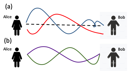
Figure 2: In (a), three quantum channels connecting two parties (Alice and Bob) with different number of qudits and transmission probabilities required to reach the threshold success probability $\overline{P}_{S}$ for the 7-qudits QRS code. In (b), the same threshold probability can be reached with the aggregating network approach in which Alice and Bob are now connected by two channels having less transmission probability than the blue and red channel or less qudits per channel than the blue and black channel.

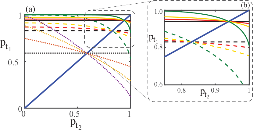
Figure 3: (a) Photon transmission probabilities required to reach $\overline{P}_{S}$ for different QRS codes. The dotted curves correspond to the quantum multiplexing 211-qudit QRS case, in which each photon is carrying 8 qubits, where all qudits are traveling in the same channel (black), 50 (orange), 80 (yellow) and 100 (purple) qudits are traveling in the channel having transmission probability $p_{t_{2}}.$ The solid (dashed) curves refer to the no multiplexing (multiplexing) case for the 43 qudits QRS code. The black curves are the cases when all qudits are traveling in the same channel. The red, yellow and green curves are, respectively, the cases when 5, 10 and 20 qudits are traveling in the channel with transmission probability $p_{t_{2}}.$ In (b), a zoom of (a) that highlights the advantage of using the aggregation network approach for a range of values of the transmission probabilities of the 43-qudit QRS code.

A natural question that arises now is what the overall success probability when multiple channels are used in an aggregative fashion. It is illustrative here to explore the 2 channels example. Here we will assume that all photons are encoding a specific qudit and propagate in one of these 2 channels. In this case, the overall success probability is

$$\begin{array}[]{c}P_{S}\left(2\mathrm{ch}\right)=\sum_{i=0}^{(d-1)/2}\sum_{j=0}^{i}{n\choose{i-j}}P_{t_{2}}^{n-(i-j)}(1-P_{t_{2}})^{i-j}\\ \times{d-n\choose{j}}P_{t_{1}}^{d-n-j}(1-P_{t_{1}})^{j},\end{array}$$ (3)

where $P_{t_{2}}=p_{t_{2}}^{\lceil\frac{\log_{2}(d)}{q}\rceil}$ is the transmission probability of all qudits encoded with photons traveling in the lossy channel with transmission probability $p_{t_{2}}.$ This is valid for both the multiplexed and unmultiplexed cases.

The example we have explored so far uses few qudits and requires rather high transmission probabilities. To move to more realistic situations in which the transmission probabilities can be much lower we need to increase the size the error correction code. The 43 qudit QRS error correcting code is a nice compromise here as it allows us to explore situations in which, by increasing the quality of one channel, we can largely decrease the quality of the other. Figure 3(b) shows the transmission probabilities required to reach $\overline{P}_{S}$ for QRS error correction code for different cases. The solid (dashed) curves corresponds to the no-multiplexing (multiplexing) cases respectively. In the multiplexing case we assume that all photons are carrying 4 qubits each. The black curves refer to the situation in which all photons are traveling in the same channel while the red, yellow and green curves show the cases in which 5, 10 and 20 qudits are traveling in the second channel respectively.

Let us now explore this behavior in more detail. For the no-multiplexing case Fig. 3(b) shows that all curves are crossing at $p_{t_{2}}\simeq 0.94,$ as expected. This is the value for reaching $\overline{P}_{S}$ when all photons are traveling in the same channel (solid black line). The advantage of using another channel, represented by the green (and other color) curves is that by slightly increasing one channel transmission probability we can considerably decrease the other. For instance the green curve shows in the case where channel 2 carries 20 qudits we can by increasing $p_{t_{2}}$ by approximately $5\%$ to $\sim 0.99$ reduce $p_{t_{1}}$ by $\sim 13.8\%$ to $0.81.$ This is a significant change in the characteristics of the channels. This reduction is even more evident for the multiplexing case represented by the dashed curves in Fig. 3(b). Here the black dashed curve corresponds to $p_{t_{2}}=0.83$ while the green dashed curve illustrates the situation with 20 qudits traveling in the second channel. As an extreme example by improving $p_{t_{2}}$ to $0.99$ $(\sim 19.2\%\,\mathrm{increase})$ we can decrease $p_{t_{1}}$ to $0.39$ $(\sim 53\%\,\mathrm{lower})$. Alternatively we could increase $p_{t_{2}}$ to 0.9 $(\sim 8.4\%\,\mathrm{increase})$ which in turn allows us to decrease $p_{t_{1}}$ to $0.757$ $(\sim 8.8\%\,\mathrm{lower}).$ Here the aggregate network approach allows to reduce the capacity of one channel more than the amount the transmission efficiency of the other channel must be increased. This advantages is enhanced by applying the quantum multiplexing technique.

Further quantum multiplexing allows to use less photons as well as less qubits with significant improvements seen as we move to higher multiplexing degrees Lo Piparo et al. (2020). However, using photons carrying an higher number of qubits is not always a convenient strategy to diminish the number of resources. A practical example will explain clearly this statement. In the 7-qudit code, each qudit can be encoded by 3 photons as well as by one photon carrying 3 qubits. Hence multiplexing the photons by adding an extra qubit, will not be beneficial for the code because this extra qubit is irrelevant for the encoding of the qudit and it could be only possibly used to encode a different qudit. If this happens the loss of this specific photon will destroy both qudits greatly lowering the success probability. Regardless one can think of an alternative scenario which we describe in the next Section.

IV Quantum network aggregation - II

As highlighted above the loss of a photon that encodes a qudit will result in the loss of the qudit itself. Therefore when quantum multiplexing is used it is critical that all the qubits of a single photon are encoding the same qudit rather than two (or more) qudits. In this way, the loss of that photon will not affect the loss of two (or more) qudits. Now by using the aggregating network technique we have a significant advantage in distributing the qubits of the same photon over different qudits. This is our second scenario.

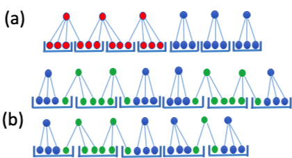
Figure 4: Pictorial representation of the second aggregate networks scenario in which multiplexed photons (dots outside the boxes) are encoding different qudits (boxes) for (a) the 7-qudits QRS code and for (b) the 11-qudits QRS code. In (a) ((b)) the red (green) dots are the photons traveling in the higher quality channel. Each qudit is encoded with the qubits (dots inside the boxes) linked to the corresponding photon.

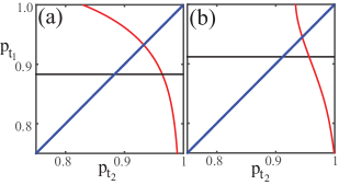
Figure 5: In (a)((b)), the black curve is the transmission probability of the 7(11)-qudit QRS code required to reach the threshold success probability when all photons are carrying 3(2) qubits each. The red curve gives the nominal values of the transmission probabilities required to reach the threshold success probability of two channels for the code represented in Fig. 4(a)((b)), respectively.

In this second scenario we assume that multiplexed photons can simultaneously encode different qudits. In order to compensate for the detrimental effect arising from loss of such photons they must travel in the higher quality channel. This scenario is illustrated in Fig. 4(a)((b)) where 6 photons carrying 4 and 3 qubits of information are encoding seven qudits and in which 15 photons are encoding 11 qudits, respectively. In Fig. 4(a) we consider the situation where the red photons are traveling in the better channel whereas in Fig. 4(b) the green photons are traveling in the better channel where they encode 2 qudits. Assigning the photons encoding multiple qudits to the higher transmitivity channel means that the information has better chance to successfully propagate to the end of the channel while keeping the success probability of the QRS code high. We have two success probabilities of interest: first $P_{S_{6}}(2\mathrm{ch})$ representing the situation shown in Fig. 4(a) and second $P_{S_{15}}(2\mathrm{ch})$ representing the situation shown in Fig. 4(b). These probabilities are explicitly given by

$$\begin{array}[]{c}P_{S_{6}}(2\mathrm{ch})=p_{t_{1}}^{3}p_{t_{2}}^{3}+{3\choose{1}}p_{t_{2}}^{2}(1-p_{t_{2}})p_{t_{1}}^{3}+{3\choose{1}}p_{t_{1}}^{2}(1-p_{t_{1}})p_{t_{2}}^{3}\\ +{3\choose{1}}p_{t_{2}}^{2}(1-p_{t_{2}}){3\choose{1}}p_{t_{1}}^{2}(1-p_{t_{1}})+{3\choose{2}}p_{t_{2}}(1-p_{t_{2}})^{2}p_{t_{1}}^{3}\\ +{3\choose{2}}p_{t_{2}}^{3}(1-p_{t_{1}})^{2}p_{t_{1}}+p_{t_{2}}^{3}(1-p_{t_{1}})^{3},\end{array}$$ (4)

and

$$\begin{array}[]{c}P_{S_{15}}(2\mathrm{ch})=p_{t_{1}}^{8}p_{t_{2}}^{7}+{7\choose{1}}p_{t_{2}}^{6}(1-p_{t_{2}})p_{t_{1}}^{8}+{8\choose{1}}p_{t_{2}}^{7}(1-p_{t_{1}})p_{t_{1}}^{7}\\ +{7\choose{2}}p_{t_{2}}^{5}(1-p_{t_{2}})p_{t_{1}}^{8}+{8\choose{2}}p_{t_{2}}^{7}(1-p_{t_{1}})p_{t_{1}}^{6}\\ +{7\choose{1}}{8\choose{1}}p_{t_{2}}^{6}(1-p_{t_{2}})(1-p_{t_{1}})p_{t_{1}}^{7}+\\ \left({7\choose{3}}-20\right)p_{t_{2}}^{4}(1-p_{t_{2}})^{3}p_{t_{1}}^{8}+{8\choose{3}}p_{t_{2}}^{7}(1-p_{t_{1}})^{3}p_{t_{1}}^{5}\\ +{7\choose{2}}{8\choose{1}}p_{t_{2}}^{5}(1-p_{t_{2}})^{2}(1-p_{t_{1}})p_{t_{1}}^{7}\\ +{7\choose{1}}{8\choose{2}}p_{t_{2}}^{6}(1-p_{t_{2}})(1-p_{t_{1}})^{2}p_{t_{1}}^{6}\\ +{8\choose{4}}p_{t_{2}}^{7}(1-p_{t_{1}})^{4}p_{t_{1}}^{4}+{7\choose{1}}{8\choose{3}}p_{t_{2}}^{6}(1-p_{t_{2}})(1-p_{t_{1}})^{3}p_{t_{1}}^{5}\\ \left({7\choose{2}}{8\choose{2}}-3\left({2\choose{1}}{2\choose{1}}{6\choose{2}}+{2\choose{1}}{1\choose{1}}{5\choose{2}}\right)\right)\\ \times p_{t_{2}}^{5}(1-p_{t_{2}})^{2}(1-p_{t_{1}})^{2}p_{t_{1}}^{6}\\ +\left({7\choose{3}}{8\choose{1}}-\left(3\left({2\choose{2}}{2\choose{1}}{5\choose{1}}+{2\choose{2}}{1\choose{1}}{4\choose{2}}\right)+20{8\choose{1}}\right)\right)\\ \times p_{t_{2}}^{4}(1-p_{t_{2}})^{3}(1-p_{t_{1}})p_{t_{1}}^{7}+{8\choose{5}}p_{t_{2}}^{7}(1-p_{t_{1}})^{5}p_{t_{1}}^{3}\end{array}$$ (5)

respectively. The exact form of these probabilities depends on the configuration of distributing the qubits.

Figures 5(a) gives a comparison between the transmission probabilities required to reach $\overline{P}_{S}$ for the 7-qudit QRS code configured in two different ways. The black curve illustrates the case in which 7 multiplexed photons ($q=3)$ are traveling through the same channel while the red curve shows the probabilities for Fig. 4(a) configuration. Here the transmission probability of the better channel must be greater than 0.95 if we want to reduce the transmission probability of the second channel. This can be a quite big price to pay but the number of photons is less.

We also observe that the reduction of the number of photons increases for higher dimensional QRS codes. For instance in the 11-qudit QRS code we require 22 multiplexed photons each carrying 2 qubits in order to reach the threshold probability all of them traveling in the same channel. However we can use the configuration scheme represented in Fig. (4)(b) to achieve this with only 15 photons by using different degrees of multiplexing. This is illustrated in Fig. 5(b) (red curve) and we note that the red curve crosses the black curve which corresponds to the 11-qudits QRS code encoded by 22 multiplexed photons. These results show that by using higher degrees of multiplexing carried by the photons encoding different qudits, the threshold success probability can be still reached provided that we use the aggregate network approach. Although not explicitly shown, we expect a even further reduction of the number of photons by applying this method to higher dimensional codes. For instance, for the 43 qudits case, we require 86 photons each of them carrying 3 qubits traveling in the same channel and only 65 photons arranged similarly to Fig. 4(b), of which 63 photons carrying 4 qubits and 2 photons carrying 3 qubits. Moreover, this indicates that, in order to implement this second scenario, the mixing strategy, i. e. the procedure of using photons with different multiplexing degree, is a fundamental approach that must be used Lo Piparo et al. (2020). It also highlights a significant advantage this mixing strategy allows for in quantum network aggregation.

V Conclusions

Future quantum networks will allow the distribution of qubits between remote users through intermediate nodes connected by multiple paths. Such routes are likely to have insufficient resources in terms of number of qubits or channel capacity in order to achieve the successful transmission of quantum information in all the required situations. In this work we address such issues by combining our quantum aggregate network approach with the quantum multiplexing method for the quantum Reed-Solomon error correction code. We initially illustrate how the QRS code can be encoded by using photons. This allows us to apply quantum multiplexing to it, which greatly reduces the number of photons, qubits and CNOT gates required to reach a given threshold success probability. We then show however that even for the no multiplexing case one channel with higher transmission probability can compensate for the other channel with much lower transmission probability. This advantage can be further enhanced when quantum multiplexing is used. In particular for the 43-qudit QRS code, in which each photon has quantum multiplexing degree equal to 4, and 20 qudits are traveling in a higher quality channel, the transmission probability of worse channel can be decrease slightly more than 50%, while increasing the transmission probability of only 19.2 % compared to the case in which all 43 qudits are traveling in the same channel.

Further we combine this with the mixed strategy from the quantum multiplexing scheme, in which the degree of quantum multiplexing may vary for each photon. In this case the photons traveling in the better channel are encoding two qudits. Thanks to this configuration the number of photons encoding the 7-qudit and the 11-qudit QRS codes can be reduced still reaching the threshold success probability. However in this case the transmission probability of the better channel must be slightly higher than the one required for the case in which all photons are traveling in the same channel. By using this technique, when large dimensional QRS code are considered, the reduction of photons required is considerably larger.

Although not explicitly shown, the same advantages resulting from the application of this aggregation technique to the QRS code can be obtained for the quantum parity code and many other loss based quantum error correction codes. We believe that aggregate networks combined with the quantum multiplexing method can be considered as a valuable approach to alleviate the high costs required for the implementation of quantum technologies in the near future.

Appendix A The $[[3,1,2]]_{3}$ QRS code

Here we derive Eq. (1) by using the logic scheme of Fig. 1(a). We begin as shown in the Figure by initializing the three qutrits as $\left.|\psi\right\rangle_{1}=\left.\alpha|0\right\rangle+\left.\beta|1\right\rangle+\left.\gamma|2\right\rangle,$ $\left.|\psi\right\rangle_{2}=\left.|0\right\rangle$ and $\left.|\psi\right\rangle_{3}=\left.|0\right\rangle+\left.|1\right\rangle+\left.|2\right\rangle,$ respectively. We then apply the CX gate represented in Fig. 1(a) with a red box. This gate will perform the following operations on the qutrits: $\left.CX|0\right\rangle\left.|0\right\rangle=\left.|0\right\rangle\left.|0\right\rangle,$ $\left.CX|1\right\rangle\left.|0\right\rangle=\left.|1\right\rangle\left.|2\right\rangle$ and $\left.CX|2\right\rangle\left.|0\right\rangle=\left.|2\right\rangle\left.|1\right\rangle,$ respectively.

We then apply the control cyclic gate between qutrit 3 and 2 and between 3 and 1, respectively. This gate adds mod-2 $n$ units to the target qutrit, where $n$ is the state of the control qutrit. The resulting state is expressed by Eq. 1.

Appendix B The qubits encoding of the $[[3,1,2]]_{3}$ QRS code

In this Appendix we show how we can construct the $[[3,1,2]]_{3}$ QRS code using six polarized photons. It is illustrative to begin by showing how one can encode a single qutrit into to two polarization encoded photons (see Fig. 6(a)). Our initial state is of the form $\left.|\psi\right\rangle_{1}=\alpha\left.|0\right\rangle_{1}+\beta\left.|1\right\rangle_{1}$ and $\left.|\psi\right\rangle_{2}=\left.|0\right\rangle_{2}$, where $\left.|0\right\rangle=\left.|H\right\rangle$ and $\left.|1\right\rangle=\left.|V\right\rangle.$ After applying a CNOT gate and letting the second photon pass through a polarizing beam splitter (PBS) we have the two-qubit entangled state $\alpha\left.|00\right\rangle+\beta\left.|11\right\rangle.$ We now apply a second PBS to photon 2 followed by the letting the V-component pass through an unbalanced BS which add a phase $\vartheta$ to this component. The resulting state is of the form $\alpha\left.|00\right\rangle+\beta\left.\cos\vartheta|11\right\rangle\left.|0\right\rangle+\beta\left.\sin\vartheta|10\right\rangle\left.|1\right\rangle.$ The components are recombined into the same initial modes by applying two PBSs and a CNOT to give $\alpha\left.|00\right\rangle+\beta\left.\cos\vartheta|10\right\rangle+\beta\left.\sin\vartheta|11\right\rangle.$ Finally, through a swap gate we obtain the desired initial state

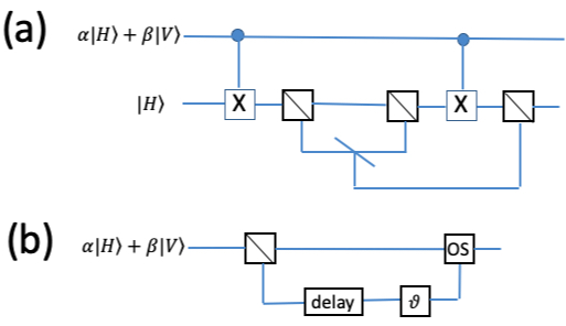
Figure 6: Logic circuit to create a qutrit using (a) two polarized photons and (b) one multiplexed photon.

$$\alpha\left.|00\right\rangle+\beta\left.\cos\vartheta|01\right\rangle+\beta\left.\sin\vartheta|11\right\rangle.$$ (6)

With this initial state we can now apply the logic circuit of Fig. 1(b) to create deterministically the desired logic qutrit $\left.|D\right\rangle$

$$\begin{array}[]{c}\begin{array}[]{c}\begin{array}[]{c}\left.|0\right\rangle_{L}=\left.|H_{1}H_{2}H_{3}H_{4}H_{5}H_{6}\right\rangle+\left.|V_{1}H_{2}V_{3}H_{4}V_{5}H_{6}\right\rangle\end{array}\\ \left.+|V_{1}V_{2}V_{3}V_{4}V_{5}V_{6}\right\rangle,\\ \left.|1\right\rangle_{L}=\left.|H_{1}H_{2}V_{3}H_{4}V_{5}V_{6}\right\rangle+\left.|V_{1}H_{2}V_{3}V_{4}H_{5}H_{6}\right\rangle\\ +\left.|V_{1}V_{2}H_{3}H_{4}V_{5}H_{6}\right\rangle,\\ \left.|2\right\rangle_{L}=\left.|H_{1}H_{2}V_{3}V_{4}V_{5}H_{6}\right\rangle+\left.|V_{1}H_{2}H_{3}H_{4}V_{5}V_{6}\right\rangle\\ +\left.|V_{1}V_{2}V_{3}H_{4}H_{5}H_{6}\right\rangle.\end{array}\end{array}$$ (7)

Appendix C Quantum multiplexing applied to the $[[3,1,2]]_{3}$ QRS code

One can consider using 3 quantum multiplexed photons (instead of 6 photons) each carrying 2 qubits to encode the $[[3,1,2]]_{3}$ QRS QEC. In this case we only need 3 photons as the total number of qubits will be the same as in the non-multiplexing case. For the second qubit we use the time-bin degree of freedom, having $S$ and $L$ as the short and long component, respectively. Accordingly, the component of the second photon required to encode one qutrit can be expressed by the time-bin components as $H\rightarrow S$ and $V\rightarrow L.$ The initial state can be created by using the logic circuit of Fig. 6(b). In this case we start with a single photon given by $\left.|\psi\right\rangle=\alpha\left.|H\right\rangle+\beta\left.|V\right\rangle.$ Applying a PBS and a delay followed by a $\vartheta$ rotation on the V component will give $\alpha\left.|H_{S}\right\rangle+\beta\left.\cos\vartheta|H_{L}\right\rangle+\beta\left.\sin\vartheta|V_{L}\right\rangle.$ An optical switch (OS) will recombine the components into the same mode to create the initial state.

Control	Target	Procedure
Polarization	Polarization	Atomic interaction
Polarization	Time-bin	Swap $H_{S_{2}}$ with $V_{L_{2}}$ CNOT Pol.1 Pol.2 Swap $H_{S_{2}}$ with $V_{L_{2}}$
Time-bin	Polarization	Swap $H_{L_{1}}$ with $V_{S_{1}}$ CNOT Pol.1 Pol.2 Swap $H_{L_{1}}$ with $V_{S_{1}}$
Time-bin	Time-bin	Swap $H_{L_{1}}$ with $V_{S_{1}}$ CNOT Pol.1 TB2 Swap $H_{L_{1}}$ with $V_{S_{1}}$

Table 1: The operations required to perform a CNOT gate between different DOFs of two quantum multiplexed photons.

In this case the corresponding logic qutrit based states of Eq. 7 will be

$$\begin{array}[]{c}\begin{array}[]{c}\left.|0\right\rangle_{L}=\left.|H_{S_{1}}H_{S_{2}}H_{S_{3}}\right\rangle+\left.|V_{S_{1}}V_{S_{2}}V_{S_{3}}\right\rangle\left.+|V_{L_{1}}V_{L_{2}}V_{L_{3}}\right\rangle\\ \left.|1\right\rangle_{L}=\left.|H_{S_{1}}V_{S_{2}}V_{L_{3}}\right\rangle+\left.|V_{S_{`1}}V_{L_{2}}H_{S_{3}}\right\rangle+\left.|V_{L_{!}}H_{S_{2}}V_{S_{3}}\right\rangle\\ \left.|2\right\rangle_{L}=\left.|H_{S_{1}}V_{L_{2}}V_{S_{3}}\right\rangle+\left.|V_{S_{1}}H_{S_{2}}V_{L_{3}}\right\rangle+\left.|V_{L_{1}}V_{S_{2}}H_{S_{3}}\right\rangle\end{array}\end{array}$$

The basic gates that allow to reproduce entirely the corresponding logic gates of Fig. 1(b) are CNOT gates between the polarization degrees of freedom (DOFs) (which we assume it can be mediated by an atom), between polarization DOF and time-bin DOF and between time-bin and time-bin DOF of two quantum multiplexed photons. Table 1 summarizes the procedure used to perform a deterministic CNOT gate between two generic DOFs of photon $1$ (Control) and photon $2$ (Target), respectively. The swapping of the components can be performed by using linear optical elements are shown in the Supplemental material of Lo Piparo et al. (2020). Finally, the Toffoli gates in Fig. 1(b) can be decomposed as a series of single qubits rotation and a single CNOT gate between the DOFs given in Table 1.

Appendix D High dimensional QRS code

In this Appendix we discuss the advantages arising from applying the aggregate network technique to the quantum multiplexing 211-qudit QRS code where each photon is carrying 8 qubits. The results for such a code are illustrated in Figure 3(a). Here the black dotted curve is the transmission probability required to reach $\overline{P}_{S}$ when all qudits are traveling in the same channel. The colored curves correspond to the aggregate network case where 50 (orange), 80 (yellow) and 100 (purple) qudits are traveling in the higher transmitivity channel.