Foliated Quantum Field Theory of Fracton Order

Abstract

We introduce a new kind of foliated quantum field theory (FQFT) of gapped fracton orders in the continuum. FQFT is defined on a manifold with a layered structure given by one or more foliations, which each decompose spacetime into a stack of layers. FQFT involves a new kind of gauge field, a foliated gauge field, which behaves similar to a collection of independent gauge fields on this stack of layers. Gauge invariant operators (and their analogous particle mobilities) are constrained to the intersection of one or more layers from different foliations. The level coefficients are quantized and exhibit a duality that spatially transforms the coefficients. This duality occurs because the FQFT is a foliated fracton order. That is, the duality can decouple 2+1D gauge theories from the FQFT through a process we dub exfoliation.

Fracton topological order Nandkishore and Hermele (2019); Pretko et al. (2020); Vijay et al. (2015, 2016); Haah (2011); Bravyi et al. (2011) is a phase of matter that exhibits particles with mobility constraints. Such particles include fractons, lineons, and planons, which are energetically constrained to 0-dimensional, 1-dimensional, and 2-dimensional spatial submanifolds when isolated from other excitations. Fracton research has been motivated as a means for more robust quantum information storage Haah (2011); Bravyi and Haah (2013); Brown et al. (2016), novel dynamics Chamon (2005); Prem et al. (2017); Pai et al. (2019); Gromov et al. (2020); Pai and Pretko (2019); He et al. (2020); Dubinkin et al. (2020); Shackleton and Scheurer (2020); Feldmeier et al. (2020); Yuan et al. (2020), toy models for holography Yan (2019, 2020), exotic materials and fluids Yan et al. (2020); Pretko and Radzihovsky (2018); Pretko et al. (2019); Halász et al. (2017); Fuji (2019); Slagle and Kim (2017a); Prem et al. (2018); Nguyen et al. (2020); Doshi and Gromov (2020); Pankov et al. (2007); Xu and Wu (2008); Sous and Pretko (2020); You and von Oppen (2019), and connections to quantum gravity Pretko (2017a).

In this work, we focus on gapped type-I Vijay et al. (2016) fracton models that do not have any gauge-invariant fractal operators Ifo . The mobility constraints Shirley et al. (2019) and other important properties Shirley et al. (2019); Pai and Hermele (2019) of these models have a fundamental dependence on a layering structure of spacetime, known as a foliation structure Shirley et al. (2018), see Fig. 1. Refs. Aasen et al. (2020); Wen (2020); Wang (2020); Slagle et al. (2019a) have shown that these fracton phases can be thought of as a topological quantum field theory (TQFT) that is embedded with stacks of interfaces (also called defects) upon which certain anyons are condensed. These interfaces are the so-called leaves (i.e. layers) of the foliation. Therefore, instead of coupling to a metric $g_{\mu\nu}$, these fracton phases are coupled to one or more foliations. For example, the X-cube model Vijay et al. (2016) on a simple cubic lattice is coupled to three flat foliations, but more generic foliations are also allowed Shirley et al. (2018); Slagle and Kim (2018). This is in contrast to TQFT (without interfaces or defects), which does not couple to a metric or foliation.

Previous works have uncovered field theories for the X-cube and other gapped fracton models Slagle and Kim (2017b); Slagle et al. (2019a); Seiberg and Shao (2021); Gorantla et al. (2020); Fontana et al. (2020); You et al. (2020a, b). In Ref. Slagle et al. (2019a), the X-cube fracton model was generalized to manifolds with arbitrary curved foliations, but formally quantizing the field theory was left as an open problem. Ref. Seiberg and Shao (2021) later showed how to formally treat the X-cube field theory from Ref. Slagle and Kim (2017b) as a quantum field theory (QFT) with quantized coefficients.

In this work, we wish to quantize the foliated field theory from Ref. Slagle et al. (2019a). This task is nontrivial and requires new ideas, such as the introduction of a new kind of foliated gauge field, which behaves like a stack of ordinary gauge fields. We call a QFT with foliated gauge fields a foliated quantum field theory (FQFT).

We also show that the FQFT is a foliated fracton order Cfo ; Shirley et al. (2018, 2020, 2019). Foliated fracton orders have ground states for which a local unitary transformation can decouple 2D topological orders from the ground state. In the FQFT, this transformation exhibits an IR duality that decouples 2+1D gauge theories from the FQFT by giving a coupling constant a piecewise spatial dependence which can be manipulated by the duality.

In the following, we begin by reviewing how to mathematically describe a foliation using a 1-form foliation field. We then introduce the FQFT and discuss its gauge invariant operators, level quantization, and foliated fracton order. Some technical details and extended discussions appear in the Appendix. See Ref. Slagle for a recorded talk.

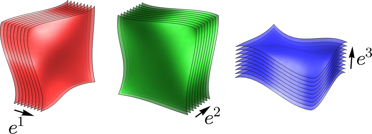
Figure 1: A depiction of some leaves (colored surfaces) for three different foliations. A foliation consists of an infinite number of infinitesimally-spaced layers, which are called leaves.

I Foliation Field

A foliation is a decomposition of a manifold into an infinite number of disjoint lower-dimensional submanifolds called leaves. A common example is to decompose 3+1D spacetime into 3D spatial slices; in this example, the codimension-1 leaves can be indexed by the time coordinate.

We will describe a codimension-1 foliation using a 1-form foliation field $e_{\mu}$. The foliation field is analogous to a metric $g_{\mu\nu}$, except $e_{\mu}$ describes a foliation geometry instead of a Riemannian geometry. The leaves of the foliation are defined to be the codimension-1 submanifolds that are orthogonal to the foliation field. That is, the tangent vectors $v^{\mu}$ of the leaves are in the null space of the foliation field covector: $v^{\mu}e_{\mu}=0$. In order for this definition to work, the foliation field must never be zero [$e(x)\neq 0\;\,\forall x$] and it must satisfy the following constraint:

$$e\wedge de=0$$ (1)

(which can be viewed as a special case of the Frobenius theorem Frankel (2011)).

More intuition can be obtained by noting that the foliation is invariant under a “gauge transformation” that rescales the foliation field (since this does not affect orthogonality to the leaves):

$$e\to\gamma e$$ (2)

where $\gamma$ is a scalar function. It is always possible to apply the above transformation such that within an open ball of spacetime, the foliation fields are closed $(de=0)$ and can be written as the derivative of a scalar function $f$: $e=df$. Locally, $f$ can be thought of as a coordinate that indexes the leaves of the foliation, similar to how a time coordinate indexes time slices of spacetime.

To foliate a torus, the foliation field can be chosen to be closed (e.g. $e=dx$ so that $de=0$). For more exotic foliations, the exterior derivative takes the form $de=e\wedge\beta$ [which satisfies Eq. (1)] for some 1-form $\beta$. The cohomology class of $\beta\wedge d\beta$ is the so-called Godbillon-Vey invariant of the foliation Godbillon and Vey (1971); Kotschick (2001), which classifies the obstruction to a closed foliation field. Under $e\to\gamma e$ [from Eq. (2)], $\beta$ transforms as $\beta\to\beta-d\gamma$.

Multiple simultaneous foliations $e^{k}$ are indexed by the superscript $k=1,2,\ldots,{n_{\text{f}}}$ (Fig. 1). Each foliation satisfies Eq. (1) independently: $e^{k}\wedge de^{k}=0$. We never implicitly sum over repeated foliation indices $k$.

II Foliated QFT

The foliated QFT (FQFT) Lagrangian is

$$L=\sum_{k=1}^{{n_{\text{f}}}}\frac{M_{k}}{2\pi}(dB^{k}+n_{k}b)\wedge A^{k}+\frac{N}{2\pi}b\wedge da$$ (3)

$$A^{k}\wedge e^{k}=0$$ (4)

$B^{k}$ and $a$ are 1-form gauge fields. (Note that $B^{k}$ is not a magnetic field in this notation; $B^{k}$ has no dependence on $A^{k}$.) $b$ is a 2-form gauge field. $A^{k}$ are foliated (1+1)-form gauge fields, which are locally 2-forms that obey the constraint Eq. (4). In Sec. II.3, we will show that the physics is equivalent under $n_{k}\sim n_{k}+N$ and that $M_{k},n_{k},N\in\mathbb{Z}$ are quantized level coefficients with $m_{k}\equiv\frac{n_{k}M_{k}}{N}\in\mathbb{Z}$ (and $M_{k}\neq 0$ and $N\neq 0$). $\sum_{k=1}^{{n_{\text{f}}}}$ sums over the different foliations. Unlike the dynamical gauge fields ($A^{k}$, $B^{k}$, $a$, $b$), the foliation field $e_{\mu}$ is non-dynamical and is not integrated over in the partition function (analogous to a static metric $g_{\mu\nu}$). Similar to a TQFT, FQFT does not couple to a metric.

If $n_{k}=0$, the second term in $L$ describes a 3+1D BF theory (which is a field theory for $Z_{N}$ gauge theory or 3D toric code Dfo ), while the first term is an FQFT for a stack of infinitesimally-spaced 2+1D BF theories for each foliation, (i.e. a field theory for stacks of $Z_{M_{k}}$ toric codes Kitaev (2003)). When $M_{k}=N$ and $n_{k}=1$, the leaves are coupled to the 3+1D BF theory, and the resulting theory describes the ground state Hilbert space of the $Z_{N}$ X-cube model Slagle and Kim (2017b); Seiberg and Shao (2021); Vijay et al. (2016); Slagle et al. (2019a) on any foliation Jfo in the limit of infinitesimal lattice spacing. This equivalence can be demonstrated in a number of ways Gfo and will be exemplified in Sec. II.2. Some intuition from coupled-layer constructions of fracton models applies here as well Vijay (2017); Ma et al. (2017); Prem et al. (2019). A lattice model for this FQFT was given in Sec. 3 and Appendix A of Ref. Slagle et al. (2019a).

II.1 Foliated Gauge Field

Foliated Gauge Field: The foliated QFT includes a new kind a gauge field: a foliated (1+1)-form gauge field $A^{k}$ for each foliation $k$. A foliated (1+1)-form gauge field behaves similarly to a stack of independent 1-form gauge fields. This is desirable because when $n_{k}=0$, the first term in Eq. (3) should describe a stack of independent 2+1D gauge theories.

Locally, a foliated (1+1)-form gauge field $A^{k}$ is a 2-form gauge field that obeys the constraint Eq. (4). Similar to ordinary gauge fields, the exterior derivative $dA^{k}$ is required to be well-defined. Note that this requirement does not put any restriction on the continuity of the foliated gauge field $A^{k}$ between leaves of the foliation. For example if $e^{1}=dz$, then the constraint Eq. (4) implies that $A^{1}=\tilde{A}^{1}\wedge dz$ for some 1-form $\tilde{A}^{1}$, and $\tilde{A}^{1}$ can have arbitrary discontinuities in the z-direction since these discontinuities will not contribute to $dA^{1}$ (due to the antisymmetry induced by the wedge product). Furthermore, we allow foliated gauge fields to contain a delta-function onto a leaf. For example if $e^{1}=dz$, then $A^{1}=x\,\delta(z)\,dy\wedge dz$ is allowed. See Appendix B for a more formal definition of foliated gauge fields.

Since the first term in Eq. (3) should describe a stack of 2+1D BF theories for each $k$ with $n_{k}=0$, the gauge fields $A^{k}$ and $B^{k}$ should effectively have three components (since the 1-form gauge fields in 2+1D BF theory have three components). Considering again the example $e^{1}=dz$, we indeed see that the constraint Eq. (4) implies that the foliated (1+1)-form has exactly three components: $A^{1}=(A_{03}^{1}\,dt+A_{13}^{1}\,dx+A_{23}^{1}\,dy)\wedge dz$. The 1-form gauge field $B^{k}$ has four components ($B^{1}=B_{0}^{1}dt+B_{1}^{1}dx+B_{2}^{1}dy+B_{3}^{1}dz$). However there is a gauge symmetry $B^{k}\to\alpha^{k}$ for an arbitrary foliated (0+1)-form $\alpha^{k}$, which locally satisfies $\alpha^{k}\wedge e^{k}=0$ (i.e. locally $\alpha^{k}=\tilde{\alpha}^{k}e^{k}$ for some scalar $\tilde{\alpha}^{k}$). This makes the $dz$ component an unimportant gauge redundancy. Therefore, $A^{k}$ and $B^{k}$ both effectively have three components (for each foliation $k$), as desired.

II.2 Fractons and Gauge Invariant Operators

Fractons and Gauge Invariant Operators: The set of gauge symmetries determines the set of gauge invariant operators. In ordinary topological QFT (e.g. Chern-Simons theory), gauge invariant operators can be smoothly deformed into any shape. However, in a foliated QFT, the gauge invariant operators are often constrained to the intersection of one or more leaves of different foliations.

Gauge invariant operators can be interpreted as moving topological excitations around in spacetime. Therefore, the rigidity of the gauge invariant operators is analogous to the mobility constraints of the fracton, lineon, and planon particles.

The gauge transformations of the FQFT are

$$\begin{split}A^{k}&\to A^{k}+d\zeta^{k}\\ B^{k}&\to B^{k}+d\chi^{k}-n_{k}\mu+\alpha^{k}\\ a&\to a+d\lambda-\sum_{k}m_{k}\zeta^{k}\\ b&\to b+d\mu\end{split}$$ (5)

where $m_{k}\equiv\frac{n_{k}M_{k}}{N}$. $\chi^{k}$ and $\lambda$ are arbitrary 0-form gauge fields, while $\mu$ is an arbitrary 1-form gauge field. $\zeta^{k}$ and $\alpha^{k}$ are foliated (0+1)-form gauge fields. Locally, $\zeta^{k}$ are 1-form gauge fields that satisfy the constraint $\zeta^{k}\wedge e^{k}=0$, and similar for $\alpha^{k}$.

Consider the following string operator:

$$W=e^{\mathrm{i}\,q\oint_{\mathcal{M}_{1}^{\text{F}}}a}$$ (6)

where $\mathcal{M}_{1}^{\text{F}}$ is a 1-dimensional manifold described below. Large gauge transformations imply that the charge $q$ is an integer. A nonlocal “equation of motion” (from integrating out $b$) shows that $W=1$ when $q$ is an integer multiple of $N$ Ffo . Therefore $W$ only depends on $q$ modulo $N$. After a gauge transformation, $W\to W\exp\!\left[\mathrm{i}\oint_{\mathcal{M}_{1}^{\text{F}}}\left(d\lambda-\sum_{k}m_{k}\zeta^{k}\right)\right]$. The first term, $\oint_{\mathcal{M}_{1}^{\text{F}}}d\lambda$, is invariant if $\mathcal{M}_{1}^{\text{F}}$ is a closed loop. The second term, $\oint_{\mathcal{M}_{1}^{\text{F}}}\sum_{k}m_{k}\zeta^{k}$, is invariant if the tangent vectors $v^{\mu}$ of $\mathcal{M}_{1}^{\text{F}}$ are in the null space of each $m_{k}\zeta^{k}$, i.e. $v^{\mu}m_{k}\zeta^{k}_{\mu}=0$. But locally, $\zeta^{k}_{\mu}=\tilde{\zeta}^{k}e^{k}_{\mu}$ for some scalar $\tilde{\zeta}^{k}$. Therefore the second term is gauge invariant if for each $k$ with $m_{k}\neq 0$, the loop $\mathcal{M}_{1}^{\text{F}}$ is supported on a single leaf of the $k^{\mathrm{th}}$ foliation [since then $v^{\mu}m_{k}\zeta^{k}_{\mu}\propto v^{\mu}e^{k}_{\mu}$ and $v^{\mu}e^{k}_{\mu}=0$ by the definition of $e^{k}$ above Eq. (1)].

Therefore, if there are $n$ foliations with $m_{k}\neq 0$, then the string operator [Eq. (6)] and the particle it transports are bound to the intersection of $n$ leaves. If there are three or more spatial foliations (that are spatially transverse) as in Fig. 1, then this string operator can move fractons in time (assuming time is periodic), but it cannot move fractons spatially. When $n_{k}=1$ and $M_{k}=N$, this fracton is equivalent to the X-cube fracton Vijay et al. (2016) for any foliationJfo . It has been proven that all compact orientable 3-manifolds admit a total foliation (i.e. three transverse foliations) Hardorp (1980), which implies that all such manifolds admit an FQFT with fractons.

Consider a different string operator:

$$T=e^{\mathrm{i}\oint_{\mathcal{M}_{1}^{\text{L}}}\sum_{k}q_{k}B^{k}}$$ (7)

Large gauge transformations imply that the charges $q_{k}\in\mathbb{Z}$ are integers. The $B^{k}\to B^{k}+d\chi^{k}$ gauge transformation shows that $\mathcal{M}_{1}^{\text{L}}$ must be be a closed loop. The $B^{k}\to B^{k}+\alpha^{k}$ gauge transformation [where $\alpha^{k}=\tilde{\alpha}^{k}e^{k}$ (locally) is a foliated (0+1)-form] shows that $\mathcal{M}_{1}^{\text{L}}$ is supported on the intersection of $n$ leaves, where $n$ is the number of foliations $k$ with nonzero $q_{k}\neq 0$. Finally, the $B^{k}\to B^{k}-n_{k}\mu$ gauge transformation implies that $\sum_{k}q_{k}n_{k}=0$. Therefore, the set of allowed charge vectors forms an abelian group $G=\{q\in\mathbb{Z}^{{n_{\text{f}}}}\;|\;\sum_{k}q_{k}n_{k}=0\}$.

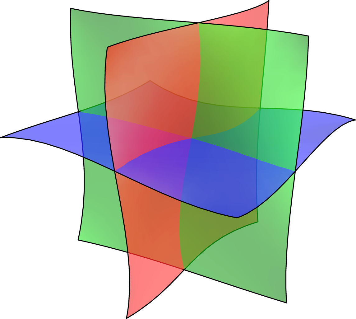
(a)

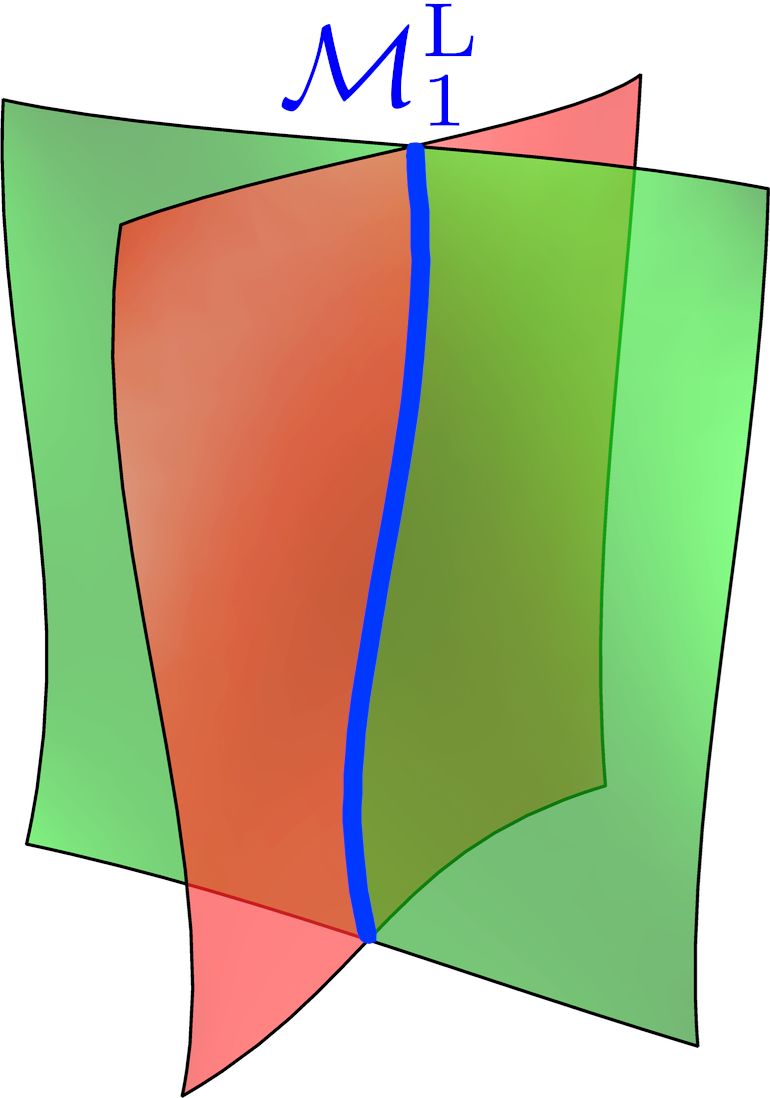
(b)

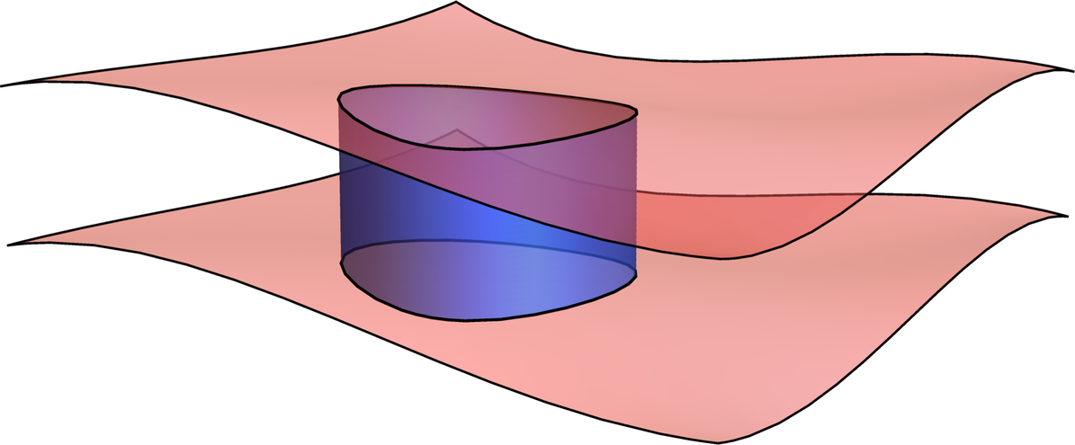
(c)

Figure 2: Spatial pictures of: (a) Three leaves intersecting at a point. (b) A 1-dimensional manifold $\mathcal{M}_{1}^{\text{L}}$ (blue) at the intersection of two leaves (red and green). (c) A 2-dimensional manifold $\mathcal{M}_{2}^{\text{P}}$ (blue) with boundaries supported on leaves (red).

A nonlocal “equation of motion” (from integrating out $A^{k}$) shows Ffo that $T=1$ when $q_{k}\in M_{k}\mathbb{Z}$ (and $\sum_{k}q_{k}n_{k}=0$). Thus, the trivial charge vectors form a subgroup $N=\{q\in G\;|\;q_{k}\in M_{k}\mathbb{Z}\}\triangleleft G$. Since both of these groups ($G$ and $N$) are isomorphic to $\mathbb{Z}^{{n_{\text{f}}}-1}$ (or $\mathbb{Z}^{{n_{\text{f}}}}$ if $n_{k}=0$), their quotient group $G/N$ of physically distinct charge vectors is a finite abelian group (i.e. $G/N$ is isomorphic to $Z_{r_{1}}\times\cdots\times Z_{r_{{n_{\text{f}}}-1}}$ for some integers $r_{i}\in\mathbb{N}$).

In the $Z_{N}$ X-cube model example with three foliations and $n_{k}=1$ and $M_{k}=N$, the allowed charge vectors are spanned by $q_{k}^{\text{(X)}}=(0,1,-1)$ and $q_{k}^{\text{(Z)}}=(1,-1,0)$. These particles are bound to a pair of leaves (Fig. 2b) and are therefore restricted to spatially only move along 1D lines (for spatial foliations). These are $Z_{N}$ X-cube lineons. For the standard three flat foliations ($e^{1}=dx$, $e^{2}=dy$, $e^{3}=dz$), $q_{k}^{\text{(X)}}$ and $q_{k}^{\text{(Z)}}$ can move only in the X and Z directions, respectively; and their sum $q_{k}^{\text{(X)}}+q_{k}^{\text{(Z)}}=(1,0,-1)$ can only move in the Z direction. This is analogous to the X-cube model where the composition of an X-axis lineon with a Z-axis lineon is a Y-axis lineon. The physics generalizes naturally to $n$ foliations: the charge vectors are spanned by $n-1$ vectors of the form $(\cdots,0,1,-1,0,\cdots)$. Note that even if a charge vector has three nonzero components, it is not a fracton; instead, it is the composition of at most two lineons.

Even for an arbitrary number of foliations and coefficients $n_{k}$, it is always possible to decompose a charge vector $q_{k}$ into lineon and planon charges (which have at most two nonzero elements $q_{k}\neq 0$). See Appendix E for a proof. Therefore, the string operator $T$ only describes lineons (or composites of lineons and planons), but never fractons.

Other gauge invariant operators include

$$T^{\prime}=e^{\mathrm{i}\oint_{\mathcal{M}_{2}}b} W^{\prime}=e^{\mathrm{i}\oint_{\mathcal{M}_{2}^{\text{P}}}A^{k}}$$ (8)

$\oint_{\mathcal{M}_{2}}b$ denotes an integral of $b$ over a closed 2-manifold $\mathcal{M}_{2}$. $\oint_{\mathcal{M}_{2}^{\text{P}}}A^{k}$ denotes an integral of $A^{k}$ over a 2-manifold $\mathcal{M}_{2}^{\text{P}}$ with boundaries that must each be supported on a single leaf of the foliation $k$, as in Fig. 2c. $T^{\prime}$ wraps a string excitation around $\mathcal{M}_{2}$. In the X-cube model example, $T^{\prime}$ measures the number of fractons inside $\mathcal{M}_{2}$. In the X-cube lattice model, this operator is a complicated operator that wraps a loop of many lineon excitations around $\mathcal{M}_{2}$. In the X-cube example, $W^{\prime}$ moves a pair of X-cube fractons around the top and bottom boundaries of the blue 2-manifold $\mathcal{M}_{2}^{\text{P}}$ shown in Fig. 2c.

See Appendix C for more general operators and a different approach to understanding the particle mobility constraints.

II.3 Level Quantization

Level Quantization: Now we study the quantization of the level coefficients $M_{k}$, $n_{k}$, and $N$. First note that $m_{k}\equiv\frac{n_{k}M_{K}}{N}$ and $n_{k}$ appear as coefficients in the gauge transformations [Eq. (5)] of compact gauge fields ($a$ and $B^{k}$). This implies that $m_{k},n_{k}\in\mathbb{Z}$.

The Lagrangian transforms under the gauge transformations [Eq. (5)] as:

$$L\to L^{\prime}=L +\sum_{k}\frac{M_{k}}{2\pi}(dB^{k}\wedge d\zeta^{k}+d\chi^{k}\wedge dA^{k})$$ (9)

$$+\frac{N}{2\pi}(db\wedge d\lambda+d\mu\wedge da)$$

Locally, the new terms are total derivatives. But since these are derivatives of gauge fields, their integral over a closed manifold can be nonzero. However, the integral is quantized such that the change in the action is an integer multiple of $2\pi M_{k}$ plus an integer multiple of $2\pi N$. Therefore, the partition function $Z=e^{i\int L}$ is gauge invariant if $M_{k},N\in\mathbb{Z}$.

The equations of motion that result from integrating out $a$ and $B^{k}$ imply Ffo that locally $db=dA^{k}=0$ and globally the operators in Eq. (8) are quantized:

$$\oint_{\mathcal{M}_{2}}b \in\frac{2\pi}{N}\mathbb{Z} \oint_{\mathcal{M}_{2}^{\text{P}}}A^{k} \in\frac{2\pi}{M_{k}}\mathbb{Z}$$ (10)

Together, these local and global equations of motion show that the $b\wedge A^{k}$ term in the FQFT action [Eq. (3)] is quantized as follows:

$$\frac{M_{k}n_{k}}{2\pi}\int b\wedge A^{k}\in 2\pi\frac{n_{k}}{N}\mathbb{Z}$$ (11)

This implies that the action is invariant under the following identification $n_{k}\sim n_{k}+N$.

III Exfoliation

Ref. Shirley et al. (2018) showed that a finite-depth local unitary transformation can map between the ground states of (1) an X-cube model of lattice length $L_{0}$ in one direction, and (2) an X-cube model of lattice length $L_{0}-1$ in the same direction along with a decoupled layer of toric code (and some trivial decoupled qubits). We will refer to this process as exfoliation. In high-energy terminology, exfoliation corresponds to an IR duality that decouples 2+1D gauge theories from a 3D FQFT. A fracton order that admits exfoliation is said to be a foliated fracton order Cfo ; Shirley et al. (2018, 2020). The X-cube model is a foliated fracton order that is foliated by toric code layers Shirley et al. (2018); Afo .

We now show that the FQFT is a foliated fracton order by exfoliating 2+1D BF theories. For simplicity, consider a flat foliation $e^{1}=dz$ (which may coexist with other foliations $e^{k}$). We want to demonstrate a duality from an FQFT with constant $n_{1}\in\mathbb{Z}$ to an FQFT with a spatially-dependent $\tilde{n}_{1}(z)$ that is zero within $z_{1}<z<z_{2}$:

$$n_{1}\leftrightarrow\tilde{n}_{1}(z)=\begin{cases}n_{1}&z\leq z_{1}\text{ or }z\geq z_{2}\\ 0&z_{1}<z<z_{2}\end{cases}$$ (12)

On the right-hand-side of the duality, the $A^{1}$ and $B^{1}$ fields within $z_{1}<z<z_{2}$ are decoupled from the rest of the fields. The equations of motion for $A^{1}$ and $B^{1}$ are $dA^{1}=dB^{1}\wedge e^{1}=0$ within $z_{1}<z<z_{2}$. These equations of motion do not contain $z$-derivatives $\partial_{z}$ [recall $A^{1}\wedge e^{1}=0$ from Eq. (4)], which shows that $A^{1}$ and $B^{1}$ at different $z$ are completely decoupled. These decoupled fields constitute an exfoliated stack of infinitesimally-spaced 2+1D BF theories.

The duality results from the following transformation:

$$a \leftrightarrow\tilde{a}=\begin{cases}a&z\leq z_{1}\text{ or }z_{2}\leq z\\ a+m_{1}\int_{z_{1}}^{z}A^{1}&z_{1}<z<z_{2}\end{cases}$$

$$A^{1} \leftrightarrow\tilde{A}^{1}=A^{1}+\delta(z-z_{2})\int_{z_{1}}^{z_{2}}dz\,A^{1}$$ (13)

$$B^{1} \leftrightarrow\tilde{B}^{1}=\begin{cases}B^{1}&z\leq z_{1}\text{ or }z_{2}\leq z\\ B^{1}-B^{1}(z_{2})+n_{1}\int_{z}^{z_{2}}b&z_{1}<z<z_{2}\end{cases}$$

We are using a notation where the integrals above are defined as $\big{(}\int_{z_{1}}^{z}A^{1}\big{)}_{\mu}\equiv\int_{z_{1}}^{z}A^{1}_{3\mu}\,dz$, $\big{(}\int_{z_{1}}^{z_{2}}dz\,A^{1}\big{)}_{\mu\nu}=\int_{z_{1}}^{z_{2}}dz\,A^{1}_{\mu\nu}$, and $\left(\int_{z}^{z_{2}}b\right)_{\mu}\equiv\int_{z}^{z_{2}}b_{3\mu}\,dz$. In order for this definition to make sense, we have implicitly chosen a flat connection to parallel transport the gauge fields. $B^{1}(z_{2})$ is shorthand for $B^{1}(t,x,y,z_{2})$, just as $B^{1}$ is shorthand for $B^{1}(t,x,y,z)$. In Appendix G, we show that the above equation transforms the equations of motion according to Eq. (12), which demonstrates the exfoliation duality.

Note that since the duality acts nonlocally on the fields, the locality of some gauge invariant operators can change. Indeed, this must occur because $\tilde{n}_{1}=0$ will result in less rigidity constraints on the gauge invariant operators. See Appendix G for examples and further discussion.

IV Conclusion

We have introduced a generic foliated QFT (FQFT) that is capable of describing a large class of foliated gapped fracton models on foliated manifolds. We also demonstrated a novel duality that spatially transforms the level coefficients, which shows that the FQFT is a foliated fracton order Cfo ; Shirley et al. (2018, 2020).

Many future directions remain. Additional terms can be added to the FQFT Lagrangian to realize more exotic fracton models Shirley et al. (2020); Williamson and Cheng (2020); Prem and Williamson (2019); Bulmash and Barkeshli (2019); Stephen et al. (2020); Tantivasadakarn and Vijay (2020); Devakul et al. (2020). The fractonic Higgs mechanism Bulmash and Barkeshli (2018); Ma et al. (2018) could be revisited now that we understand gapped fracton orders on curved foliations Shirley et al. (2018); Slagle et al. (2019a); Aasen et al. (2020); Radicevic (2019) and $U(1)$ fracton models Pretko (2017b); Rasmussen et al. (2016); Pretko (2017c); Radzihovsky and Hermele (2020); Seiberg and Shao (2020); Seiberg (2020); Pretko (2017d) on curved space Slagle et al. (2019b). Finally, FQFT could provide further insight on other works, such as the study of boundaries of fracton models Bulmash and Iadecola (2019) or models in higher dimensions Li and Ye (2020).

Appendix A Gauge Fields (Review)

Here, we review the definition of a 1-form gauge field. Mathematically, a 1-form gauge field with gauge group $G=U(1)$ is a connection on $\mathcal{M}\times G$ (or more generally a $G$-bundle $E\to\mathcal{M}$), where $\mathcal{M}$ is the spacetime manifold. Witten (2008); Dijkgraaf and Witten (1990).

This can be made more explicit by considering a good open cover of the spacetime manifold $\mathcal{M}$; i.e. consider a collection of sets $U_{i}\subset\mathcal{M}$ that cover $\mathcal{M}$ (i.e. $\cup_{i}U_{i}=\mathcal{M}$) such that finite intersections $U_{i_{1}}\cap U_{i_{2}}\cap\cdots\cap U_{i_{n}}$ are diffeomorphic to an open ball. A 1-form gauge field can then be specified by the following data and constraints Kapustin and Seiberg (2014): (1) The gauge field is locally defined on each $U_{i}$ by a 1-form $A_{(i)}$. (2) On nonempty overlaps $U_{i}\cap U_{j}$ (depicted in yellow below), the two locally defined fields $A_{(i)}$ and $A_{(j)}$ must be equal up to a gauge transformation:

$$A_{(i)}-A_{(j)}=dg_{(ij)}$$ (14)

where $g_{(ij)}$ are called transition functions. (3) On nonempty triple-overlaps $U_{i}\cap U_{j}\cap U_{k}$ (depicted in yellow below), the transition functions must satisfy the cocycle condition up to an integer multiple of $2\pi$:

$$g_{(ij)}+g_{(jk)}+g_{(ki)}\in 2\pi\mathbb{Z}$$ (15)

A 0-form gauge field $\theta$ can be similarly defined by a 0-form $\theta_{(i)}:U_{i}\to\mathbb{R}$ on each $U_{i}$ where $\theta_{(i)}-\theta_{(j)}\in 2\pi\mathbb{Z}$ on overlaps $U_{i}\cap U_{j}$. Thus, $\theta$ could alternatively be defined as a $U(1)$-valued function $\tilde{\theta}:\mathcal{M}\to U(1)$.

See also the beginning of Ref. Kapustin and Seiberg (2014) for another a review of $q$-form gauge fields and Section 2.1 of Ref. Cordova et al. (2020) for an explicit example of how to define integrals of gauge fields.

A.1 Example

Here, we review a simple example of a field configuration for a trivial $2\pi$ flux. Consider BF theory on a 2+1D torus: $L=\frac{N}{2\pi}B\wedge dA$ where $A$ and $B$ are 1-form gauge fields. Decompose the 3-torus as $\mathcal{M}_{\mathrm{t}}\times\mathcal{M}_{\mathrm{x}}\times\mathcal{M}_{\mathrm{y}}$ with lengths ${l_{\mathrm{t}}}$, ${l_{\mathrm{x}}}$, and ${l_{\mathrm{y}}}$, where $\mathcal{M}_{\mathrm{x}}$ is a circle with coordinate $x\in[0,{l_{\mathrm{x}}})$, and similar for $\mathcal{M}_{\mathrm{t}}$ and $\mathcal{M}_{\mathrm{y}}$. Then a $2\pi$ flux that is evenly spread throughout space will have

$$dA=\frac{2\pi}{{l_{\mathrm{x}}}{l_{\mathrm{y}}}}dx\wedge dy$$ (16)

To formally specify the gauge field $A$, first choose an open cover given by (Fig. 3):

$$\begin{array}[]{ccccccc}U_{1}&=&\mathcal{M}_{\mathrm{t}}&\times&(0,{l_{\mathrm{x}}})&\times&(0,{l_{\mathrm{y}}})\\ U_{2}&=&\mathcal{M}_{\mathrm{t}}&\times&[0,\frac{{l_{\mathrm{x}}}}{2})\cup(\frac{{l_{\mathrm{x}}}}{2},{l_{\mathrm{x}}})&\times&(0,{l_{\mathrm{y}}})\\ U_{3}&=&\mathcal{M}_{\mathrm{t}}&\times&(0,{l_{\mathrm{x}}})&\times&[0,\frac{{l_{\mathrm{y}}}}{2})\cup(\frac{{l_{\mathrm{y}}}}{2},{l_{\mathrm{y}}})\\ U_{4}&=&\mathcal{M}_{\mathrm{t}}&\times&[0,\frac{{l_{\mathrm{x}}}}{2})\cup(\frac{{l_{\mathrm{x}}}}{2},{l_{\mathrm{x}}})&\times&[0,\frac{{l_{\mathrm{y}}}}{2})\cup(\frac{{l_{\mathrm{y}}}}{2},{l_{\mathrm{y}}})\end{array}$$ (17)

Note that $0\in[0,{l_{\mathrm{x}}})$ while $0\notin(0,{l_{\mathrm{x}}})$. Now the gauge field can be defined by

$$A_{(1)} =A_{(3)}=\frac{2\pi}{{l_{\mathrm{x}}}{l_{\mathrm{y}}}}x\,dy$$ (18)

$$A_{(2)} =A_{(4)}=\frac{2\pi}{{l_{\mathrm{x}}}{l_{\mathrm{y}}}}\begin{cases}x\,dy&0\leq x<\frac{{l_{\mathrm{x}}}}{2}\\ (x-{l_{\mathrm{x}}})\,dy&\frac{{l_{\mathrm{x}}}}{2}<x\leq{l_{\mathrm{x}}}\end{cases}$$

with transition functions

$$g_{(12)} =g_{(14)}=g_{(32)}=\begin{cases}0&0<x<\frac{{l_{\mathrm{x}}}}{2}\\ \frac{2\pi}{{l_{\mathrm{y}}}}y&\frac{{l_{\mathrm{x}}}}{2}<x<{l_{\mathrm{x}}}\end{cases}$$ (19)

$$g_{(34)} =\begin{cases}0&0<x<\frac{{l_{\mathrm{x}}}}{2}\\ \frac{2\pi}{{l_{\mathrm{y}}}}y&\frac{{l_{\mathrm{x}}}}{2}<x<{l_{\mathrm{x}}}\text{ and }0\leq y<\frac{{l_{\mathrm{y}}}}{2}\\ \frac{2\pi}{{l_{\mathrm{y}}}}(y-{l_{\mathrm{y}}})&\frac{{l_{\mathrm{x}}}}{2}<x<{l_{\mathrm{x}}}\text{ and }\frac{{l_{\mathrm{y}}}}{2}<y\leq{l_{\mathrm{y}}}\end{cases}$$

$$g_{(13)} =g_{(24)}=0$$

Note that $A_{(i)}$ and $g_{(ij)}$ are continuous and satisfy Eq. (14) and (15). Also note that if we rescale $A_{(i)}$ and $g_{(ij)}$ by some constant $\alpha\in\mathbb{R}$, then Eq. (15) will only be satisfied if $\alpha\in\mathbb{Z}$. Therefore, the total flux $\int dA$ must be an integer multiple of $2\pi$, which is physically trivial.

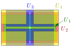
Figure 3: An XY planar slice of spacetime showing a depiction of $U_{1}$, $U_{2}$, $U_{3}$, and $U_{4}$ from Eqs. (17) and (25).

Appendix B Foliated Gauge Fields

Here, we provide a more formal definition of foliated gauge fields. See Appendix A for a review of ordinary gauge fields.

We will provide two definitions, which we believe are equivalent. The first definition is that a foliated gauge field $A$ is given by an ordinary gauge field $A_{\ell}$ on each leaf $\ell$ of a foliation. Then the integral of a foliated $(q+1)$-form gauge field $A$ over a foliated $(q+1)$-dimensional manifold $\mathcal{M}$ is given by the infinite sum of integrals over each leaf $\ell\subset\mathcal{M}$ of the foliation: $\int_{\mathcal{M}}A\equiv\sum_{\ell}\int_{\ell}A_{\ell}$.

We now provide a second definition, which avoids the infinite summation over leaves. This definition is also simpler locally (as it reduces to just a constrained 2-form gauge field). We use this second definition throughout the rest of this text. Consider a good open cover of sets $U_{i}\subset\mathcal{M}$ [as defined above Eq. (14)] that cover the spacetime manifold $\mathcal{M}$, which is foliated using a foliation field $e$, as defined in Sec. I. A foliated (1+1)-form gauge field is defined by the following data and constraints: (1) The foliated gauge field is locally defined on each $U_{i}$ by a 2-form field $A_{(i)}$ that obeys the constraint $A_{(i)}\wedge e=0$ [as in Eq. (4)]. (2) On nonempty overlaps $U_{i}\cap U_{j}$, the two locally defined fields $A_{(i)}$ and $A_{(j)}$ must be equal up to a gauge transformation:

$$A_{(i)}-A_{(j)}=dg_{(ij)}$$ (20)

where $g_{(ij)}$ is a foliated (0+1)-form transition function that obeys $g_{(ij)}\wedge e=0$. (3) On nonempty triple-overlaps $U_{i}\cap U_{j}\cap U_{k}$, these transition functions must satisfy a foliated cocycle condition:

$$\int_{s}g_{(ij)}+g_{(jk)}+g_{(ki)}\in 2\pi\mathbb{Z}$$ (21)

where $s$ is any 1D manifold (possibly with boundaries) transverse to the foliation. An example is depicted in the graphic, with $s$ drawn as a blue line.

B.1 Example

Here, we demonstrate a foliated analog of the example in Appendix A.1. That is, we wish to describe a field configuration for a trivial $2\pi$ flux on a single leaf of a foliation. We will consider the following FQFT on a 3+1D torus:

$$L=\frac{N}{2\pi}B\wedge dA$$ (22)

where $A$ is a foliated (1+1)-form gauge field and $B$ is a 1-form gauge field. This FQFT describes a foliation of 2+1D BF theories.

For the first definition, a $2\pi$ flux that is evenly spread throughout a leaf $\ell_{0}$ of the foliation will have:

$$dA_{\ell}=\begin{cases}\frac{2\pi}{{l_{\mathrm{x}}}{l_{\mathrm{y}}}}dx\wedge dy&\ell=\ell_{0}\\ 0&\ell\neq\ell_{0}\end{cases}$$ (23)

where $\ell$ indexes the different leaves of the foliation. $A_{\ell_{0}}$ can then be defined as in Appendix A.1.

Now consider the second foliated gauge field definition. For simplicity, consider a flat foliation with $e=dz$. Decompose the 4-torus as $\mathcal{M}_{\mathrm{t}}\times\mathcal{M}_{\mathrm{x}}\times\mathcal{M}_{\mathrm{y}}\times\mathcal{M}_{\mathrm{z}}$ with lengths ${l_{\mathrm{t}}}$, ${l_{\mathrm{x}}}$, ${l_{\mathrm{y}}}$, and ${l_{\mathrm{z}}}$, where $\mathcal{M}_{\mathrm{x}}$ is a circle with coordinate $x\in[0,{l_{\mathrm{x}}})$, and similar for $\mathcal{M}_{\mathrm{t}}$, $\mathcal{M}_{\mathrm{y}}$, and $\mathcal{M}_{\mathrm{z}}$. A $2\pi$ flux that is evenly spread throughout a leaf (at $z=z_{0}$) of the foliation will have:

$$dA=\frac{2\pi}{{l_{\mathrm{x}}}{l_{\mathrm{y}}}}\delta(z-z_{0})\,dx\wedge dy\wedge dz$$ (24)

To formally specify the foliated gauge field $A$, first choose an open cover given by (Fig. 3):

$$\begin{array}[]{ccccccccc}U_{1}&=&\mathcal{M}_{\mathrm{t}}&\times&(0,{l_{\mathrm{x}}})&\times&(0,{l_{\mathrm{y}}})&\times&\mathcal{M}_{\mathrm{z}}\\ U_{2}&=&\mathcal{M}_{\mathrm{t}}&\times&[0,\frac{{l_{\mathrm{x}}}}{2})\cup(\frac{{l_{\mathrm{x}}}}{2},{l_{\mathrm{x}}})&\times&(0,{l_{\mathrm{y}}})&\times&\mathcal{M}_{\mathrm{z}}\\ U_{3}&=&\mathcal{M}_{\mathrm{t}}&\times&(0,{l_{\mathrm{x}}})&\times&[0,\frac{{l_{\mathrm{y}}}}{2})\cup(\frac{{l_{\mathrm{y}}}}{2},{l_{\mathrm{y}}})&\times&\mathcal{M}_{\mathrm{z}}\\ U_{4}&=&\mathcal{M}_{\mathrm{t}}&\times&[0,\frac{{l_{\mathrm{x}}}}{2})\cup(\frac{{l_{\mathrm{x}}}}{2},{l_{\mathrm{x}}})&\times&[0,\frac{{l_{\mathrm{y}}}}{2})\cup(\frac{{l_{\mathrm{y}}}}{2},{l_{\mathrm{y}}})&\times&\mathcal{M}_{\mathrm{z}}\end{array}$$ (25)

Now the foliated gauge field can be defined by

$$A_{(1)} =A_{(3)}=\frac{2\pi}{{l_{\mathrm{x}}}{l_{\mathrm{y}}}}\delta(z-z_{0})x\,dy\wedge dz$$ (26)

$$A_{(2)} =A_{(4)}=\frac{2\pi}{{l_{\mathrm{x}}}{l_{\mathrm{y}}}}\delta(z-z_{0})\begin{cases}x\,dy\wedge dz&0\leq x<\frac{{l_{\mathrm{x}}}}{2}\\ (x-{l_{\mathrm{x}}})\,dy\wedge dz&\frac{{l_{\mathrm{x}}}}{2}<x\leq{l_{\mathrm{x}}}\end{cases}$$

with transition functions

$$g_{(12)} =g_{(14)}=g_{(32)}=\begin{cases}0&0<x<\frac{{l_{\mathrm{x}}}}{2}\\ \frac{2\pi}{{l_{\mathrm{y}}}}\delta(z-z_{0})\,y\,dz&\frac{{l_{\mathrm{x}}}}{2}<x<{l_{\mathrm{x}}}\end{cases}$$

$$g_{(34)} =\begin{cases}0&0<x<\frac{{l_{\mathrm{x}}}}{2}\\ \frac{2\pi}{{l_{\mathrm{y}}}}\delta(z-z_{0})\,y\,dz&\frac{{l_{\mathrm{x}}}}{2}<x<{l_{\mathrm{x}}}\text{ and }0\leq y<\frac{{l_{\mathrm{y}}}}{2}\\ \frac{2\pi}{{l_{\mathrm{y}}}}\delta(z-z_{0})\,(y-{l_{\mathrm{y}}})\,dz&\frac{{l_{\mathrm{x}}}}{2}<x<{l_{\mathrm{x}}}\text{ and }\frac{{l_{\mathrm{y}}}}{2}<y\leq{l_{\mathrm{y}}}\end{cases}$$ (27)

$$g_{(13)} =g_{(24)}=0$$

Note that $A_{(i)}$ and $g_{(ij)}$ satisfy Eq. (20) and (21).

Appendix C Mobility Constraints and Currents

In Sec. II.2, we studied the rigidity of the gauge invariant operators. This rigidity is analogous to the particle mobility constrains characteristic of fracton models. Consider a more general operator of the form $e^{\mathrm{i}\int L^{\prime}}$ where:

$$L^{\prime}=-\sum_{k}A^{k}\wedge J^{k}-\sum_{k}B^{k}\wedge I^{k}-a\wedge j-b\wedge i$$ (28)

$J^{k}$ and $i$ are 2-forms; $I^{k}$ is a (2+1)-form (i.e. $I^{k}\wedge e^{k}=0$); and $j$ is a 3-form. $J^{k}$, $I^{k}$, $j$, and $i$ can be thought of as current sources that parameterize the generic operator $e^{\mathrm{i}\int L^{\prime}}$.

$e^{\mathrm{i}\int L^{\prime}}$ is only gauge invariant if the following mobility constraints are satisfied:

$$dJ^{k}\wedge e^{k} =-m_{k}\,j\wedge e^{k}$$ (29)

$$dI^{k} =0,\quad I^{k}\wedge e^{k}=0$$ (30)

$$dj =0$$ (31)

$$di =\sum_{k}n_{k}I^{k}$$ (32)

These constraints result from imposing gauge invariance under the $\zeta^{k}$, $\chi^{k}$, $\alpha^{k}$, $\lambda$, and $\mu$ transformations in Eq. (5), respectively. The local foliation field constraint $A^{k}\wedge e^{k}=0$ [Eq. (4)] also results in the following redundancy: $J^{k}\to J^{k}+\phi^{k}\wedge e^{k}$, where $\phi^{k}$ is an arbitrary 1-form. This gives $J^{k}$ the same number of degrees of freedom as a (2+1)-form. Bfo

When the FQFT describes $Z_{N}$ X-cube (i.e. when $n_{k}=1$ and $M_{k}=N$ with three foliations): $j$ is the fracton current, $J$ is a fracton dipole current, linear combinations of $I$ currents result in lineons, and $i$ is a current for string excitations which do not appear in the X-cube model.

Eq. (29) tells us that any $j$ current that passes through a leaf of a foliation must be compensated by the divergence of $J$ current. This is analogous to the X-cube model where moving a fracton ($j$ current) requires creating fracton dipoles ($J$ divergence).

Eq. (32) implies that the $i$ current describes string excitations. If there are no string excitations (i.e. if $di=0$), then Eq. (32) implies that $\sum_{k}I^{k}=0$. This implies that $I$ current must come in pairs. $I^{k}\wedge e^{k}=0$ [Eq. (30)] implies that the $I$ current can only move along a leaf of the $k^{\text{th}}$ foliation. But since $I$ current must come in pairs for different foliations $k$, a particle of $I$ current must be bound to two leaves for two different foliations, which implies that $I$ describes currents of lineons.

Appendix D Equations of Motion

The equations of motion for the FQFT Lagrangian coupled to source currents, $L+L^{\prime}$ [Eqs. (3) and (28)], are given below:

$$\frac{M_{k}}{2\pi}(dB^{k}+n_{k}b)\wedge e^{k} =J^{k}\wedge e^{k}$$ (33)

$$\frac{M_{k}}{2\pi}dA^{k} =I^{k}$$ (34)

$$\frac{N}{2\pi}db =j$$ (35)

$$\frac{N}{2\pi}(da+\sum_{k}m_{k}A^{k}) =i$$ (36)

D.1 Quantized Integrals

Since the gauge fields are compact, there are also nonlocal “equations of motion” that result in quantized integrals.

For example, let us derive the following quantized period from the main text [Eq. (10)]:

$$\oint_{\mathcal{M}_{2}}b\in\frac{2\pi}{N}\mathbb{Z}$$ (37)

where $\mathcal{M}_{2}$ is a closed 2-manifold. If $\mathcal{M}_{2}$ is contractible, then $\oint_{\mathcal{M}_{2}}b=0$ by the local equation of motion $db=0$ (35). Consider a simple example of non-contractible $\mathcal{M}_{2}$ on a spacetime manifold that is an ${l_{\mathrm{t}}}\times{l_{\mathrm{x}}}\times{l_{\mathrm{y}}}\times{l_{\mathrm{z}}}$ 4-torus. Let $\mathcal{M}_{2}$ be a tz-plane. Now consider summing over field configurations with flux

$$f_{Q}=da=Q\frac{2\pi}{{l_{\mathrm{x}}}{l_{\mathrm{y}}}}\,dx\wedge dy$$ (38)

for all $Q\in\mathbb{Z}$ (similar to the example in Appendix A.1). Summing over this subset of field configurations shows that the partition function is zero unless the following integral is quantized: $\int\frac{N}{2\pi}b\wedge da\in 2\pi\mathbb{Z}$. Therefore, $\int\frac{N}{2\pi}b\wedge da=\int\frac{N}{2\pi}b\wedge f_{Q}=Q\frac{N}{{l_{\mathrm{x}}}{l_{\mathrm{y}}}}\int_{x,y}\int_{t,z}b_{03}=QN\int_{\mathcal{M}_{2}}b\in 2\pi\mathbb{Z}$, where the last equality follows because the integral of $b$ over any tz-plane will be equal due to the equation of motion $db=0$ (35). This demonstrates the quantization (37).

We now derive the other quantized period in Eq. (10):

$$\oint_{\mathcal{M}_{2}^{\text{P}}}A^{k}\in\frac{2\pi}{M_{k}}\mathbb{Z}$$ (39)

Consider the simple but nontrivial example where $\mathcal{M}_{2}^{\text{P}}$ is a tz-plane of a spacetime 4-torus, and suppose that the first foliation field is $e^{1}=dz$. Then similar to Eq. (38), we can sum over fluxes $dB^{1}=Q\frac{2\pi}{{l_{\mathrm{x}}}{l_{\mathrm{y}}}}\,dx\wedge dy$ for all $Q\in\mathbb{Z}$ and apply $dA^{1}=0$ [Eq. (34)] to derive Eq. (39) with $k=1$.

We now derive the following quantized period:

$$\oint_{\mathcal{M}_{1}^{\text{F}}}a\in\frac{2\pi}{N}\mathbb{Z}$$ (40)

where $\mathcal{M}_{1}^{\text{F}}$ is supported on a single leaf for each foliation with $n_{k}\neq 0$ [as in Eq. (6)]. Consider the simple but nontrivial example where $\mathcal{M}_{1}^{\text{F}}$ is a loop around a periodic time direction and centered at the origin of the spatial manifold $\mathbb{R}^{3}$. Then Eq. (40) will result from summing over fluxes $db=Q\,2\pi\,\delta^{3}({\bf x})\,dx\wedge dy\wedge dz$ for all $Q\in\mathbb{Z}$ and choosing $B^{k}$ such that $dB^{k}+n_{k}b=0$. These fluxes can be realized by $b=-Q\,\frac{1}{2}d(\cos\theta)\wedge d\phi$ and $B^{k}=n_{k}Q\,\frac{1}{2}(\cos\theta-1)\,d\phi$ in spherical coordinates. Summing over this subset of field configurations shows that the partition function is zero unless $\int L\in 2\pi\mathbb{Z}$, where $\int L=-\int\frac{N}{2\pi}db\wedge a=QN\int_{\mathcal{M}_{1}^{\text{F}}}a$. This demonstrates the quantization Eq. (40).

Finally, we derive the following quantized period${}^{\ref{foot:removed}}$:

$$\oint_{\mathcal{M}_{1}^{\text{L}}}\sum_{k}q_{k}B^{k}\in 2\pi\mathbb{Z}\text{ when }q_{k}\in M_{k}\mathbb{Z}$$ (41)

where $\sum_{k}q_{k}n_{k}=0$ and $\mathcal{M}_{1}^{\text{L}}$ is supported on a single leaf for each foliation with $q_{k}\neq 0$ [as in Eq. (7)]. Consider the simple but nontrivial example where $\mathcal{M}_{1}^{\text{L}}$ is a loop around a periodic time direction and centered at the origin of the spatial manifold $\mathbb{R}^{3}$. Then Eq. (41) will result from summing over fluxes $dA^{k}=\frac{q_{k}}{M_{k}}F_{Q}$ where $F_{Q}=Q\,2\pi\,\delta^{3}({\bf x})\,dx\wedge dy\wedge dz$ for each $Q\in\mathbb{Z}$ with $a_{\mu}$ chosen such that $da+\sum_{k}m_{k}A^{k}=0$. To realize the flux $dA^{k}$, consider the example foliation $e^{1}=dz$; then $A^{1}=Q\frac{q_{1}}{M_{1}}\delta(z)\,d\phi\wedge dz$ in polar coordinates (where $q_{k}\in M_{k}\mathbb{Z}$). Then $d\left(\sum_{k}m_{k}A^{k}\right)=\sum_{k}m_{k}\frac{q_{k}}{M_{k}}F_{Q}=\frac{1}{N}F_{Q}\sum_{k}q_{k}n_{k}=0$; therefore, it is possible to choose $a_{\mu}$ such that $da+\sum_{k}m_{k}A^{k}=0$. Summing over this subset of field configurations shows that the partition function is zero unless the following integral is quantized: $\int L=\int\sum_{k}\frac{M_{k}}{2\pi}B^{k}\wedge dA^{k}+\frac{N}{2\pi}b\wedge\left(da+\sum_{k}m_{k}A^{k}\right)=\int\sum_{k}q_{k}B^{k}\wedge\frac{1}{2\pi}F_{Q}=Q\int_{\mathcal{M}_{1}^{\text{L}}}\sum_{k}q_{k}B^{k}\in 2\pi\mathbb{Z}$.

Appendix E Lineon Operator

Consider the string operator $T$ in Eq. (7) with a charge vector $q_{k}$ such that $\sum_{k}q_{k}n_{k}=0$. Below, we prove that this charge vector can always be decomposed into a sum of lineon and planon charge vectors (which have at most two nonzero elements).

To prove this, first extract all planon charges $q^{(k^{\prime})}_{k}\equiv q_{k}\delta_{k,k^{\prime}}$ from the charge vector $q_{k}$:

$$q_{k}=q^{\prime}_{k}+\sum_{k^{\prime}\in K_{\text{P}}}q^{(k^{\prime})}_{k}$$ (42)

$\sum_{k^{\prime}\in K_{\text{P}}}$ sums over all foliations $k^{\prime}$ such that $q_{k^{\prime}}\neq 0$ and $n_{k^{\prime}}=0$. We are left with a new charge vector $q^{\prime}_{k}$, such that $q^{\prime}_{k}=0$ for all $k$ with $n_{k}=0$. Next, we show that $q^{\prime}_{k}$ can be decomposed into lineons.

If $q^{\prime}_{k}$ has at most two nonzero components, then $q^{\prime}_{k}$ is a lineon and the proof is complete. Otherwise, without loss of generality (by reordering the foliations $k$), assume that $q^{\prime}_{1}\neq 0$. Next, we show that $q^{\prime}_{k}$ can be decomposed into $q^{\prime\prime}_{k}$ and lineon charge vectors $q^{(1,k^{\prime})}_{k}$:

$$q^{\prime}_{k}=q^{\prime\prime}_{k}+\sum_{k^{\prime}\in K_{\text{L}}}q^{(1,k^{\prime})}_{k}$$ (43)

$\sum_{k^{\prime}\in K_{\text{L}}}$ only sums over foliations $k^{\prime}=2,3,\cdots,{n_{\text{f}}}$ such that $q^{\prime}_{k^{\prime}}\neq 0$. $q^{(1,k^{\prime})}_{k}\neq 0$ only for $k=1$ and $k=k^{\prime}$. Also note that all charge vectors in this proof ($q_{k}$, $q^{\prime}_{k}$, $q^{\prime\prime}_{k}$, $q^{(k^{\prime})}_{k}$, and $q^{(1,k^{\prime})}_{k}$) are valid charge vectors (i.e. $\sum_{k}q^{\prime}_{k}n_{k}=0$, and similar for the other charge vectors). We want to choose the $q^{(1,k^{\prime})}_{k}$ such that $q^{\prime\prime}_{1}=0$ and $q^{\prime\prime}_{k}=0$ for each $k$ with $q^{\prime}_{k}=0$. Then $q^{\prime\prime}_{k}$ will have at least one more zero element than $q^{\prime}_{k}$. Thus, we can complete the proof by repeatedly reapplying the logic of this paragraph (with $q^{\prime\prime}_{k}\to q^{\prime}_{k}$) until $q^{\prime}_{k}$ is a lineon with two nonzero components.

We now just need to show that the decomposition in Eq. (43) is possible. Without loss of generality, assume $n_{k}\neq 0$ and $q^{\prime}_{k}\neq 0$ for all foliations $k$ (by just ignoring foliations $k$ for which this is not true). Let

$$q^{(1,k^{\prime})}_{k} =Q^{(k^{\prime})}\begin{cases}+r_{k^{\prime},1}&k=1\\ -r_{1,k^{\prime}}&k=k^{\prime}\\ 0&\text{otherwise}\end{cases}$$ (44)

$$r_{k,k^{\prime}} \equiv\frac{n_{k}}{\gcd(n_{k},n_{k^{\prime}})}$$ (45)

for some integers $Q^{(k^{\prime})}$. $\gcd$ denotes the greatest common divisor. We want $\sum_{k^{\prime}=2}^{{n_{\text{f}}}}q^{(1,k^{\prime})}_{1}=q^{\prime}_{1}$ so that $q^{\prime\prime}_{1}=0$ in Eq. (43). By appropriately choosing $Q^{(k^{\prime})}\in\mathbb{Z}$, the sum $\sum_{k^{\prime}=2}^{{n_{\text{f}}}}q^{(1,k^{\prime})}_{1}$ can be any integer multiple of $R_{1}\equiv\gcd(r_{2,1},r_{3,1},\cdots r_{{n_{\text{f}}},1})$. Therefore, we just need to show that $q^{\prime}_{1}$ is an integer multiple of $R_{1}$. But $q^{\prime}_{1}n_{1}=uR$ where $R\equiv\gcd(n_{2},n_{3},\cdots n_{n_{\text{f}}})$ for some $u\in\mathbb{Z}$ since $\sum_{k}q_{k}n_{k}=0$. Thus, $q^{\prime}_{1}=\frac{uR}{n_{1}}=[u\gcd(R,n_{1})/n_{1}]\,[R/\gcd(R,n_{1})]$ is an integer multiple of $R/\gcd(R,n_{1})$. But $R/\gcd(R,n_{1})=R_{1}$ (by properties of $\gcd$ and integer division). Therefore, $q^{\prime}_{1}$ is an integer multiple of $R_{1}$, which completes the proof.

Appendix F Entanglement RG

Entanglement RG Vidal (2007) studies coarse graining by using a local unitary transformation to decouple degrees of freedom from a ground state.

For example, a local unitary can be used to coarse-grain the ground state (GS) of toric code on a periodic $2L\times 2L$ lattice to the toric code GS on a periodic $L\times L$ lattice along with decoupled qubits Aguado and Vidal (2008):

$$U\;|2L\times 2L\text{ toric code GS}\rangle$$

$$=$$ (46)

$$|L\times L\text{ toric code GS}\rangle\otimes|\underbrace{\uparrow\cdots\uparrow}_{\times 6L^{2}}\rangle$$

In a 3D foliated fracton order, the local unitary decouples 2D topological orders in addition to decoupled qubits. For example, slightly coarse-graining the X-cube model in one direction exfoliates a decoupled layer of toric code Shirley et al. (2018); Dua et al. (2020):

$$U\;|L_{x}\times L_{y}\times L_{z}\text{ X-cube GS}\rangle$$

$$=$$ (47)

$$|L_{x}\times L_{y}\times(L_{z}-1)\text{ X-cube GS}\rangle\otimes$$

$$|L_{x}\times L_{y}\text{ toric code GS}\rangle\otimes|\underbrace{\uparrow\cdots\uparrow}_{\times L_{x}L_{y}}\rangle$$

A local unitary can also be used to exfoliate every other layer:

$$U\;|L_{x}\times L_{y}\times L_{z}\text{ X-cube GS}\rangle$$

$$=$$ (48)

$$|L_{x}\times L_{y}\times\frac{L_{z}}{2}\text{ X-cube GS}\rangle$$

$$\otimes_{k=1}^{L_{z}/2}|L_{x}\times L_{y}\text{ toric code GS}\rangle\otimes|\underbrace{\uparrow\cdots\uparrow}_{\times L_{x}L_{y}\frac{L_{z}}{2}}\rangle$$

Entanglement RG is convenient for exactly solvable lattice models since the RG can often be done exactly using a simple formalism. Entanglement RG is also useful because it only discards degrees of freedom after they have been explicitly decoupled. This is in contrast to Wilsonian RG, where one could (in principal) accidentally integrate out important degrees of freedom.

Appendix G Exfoliation

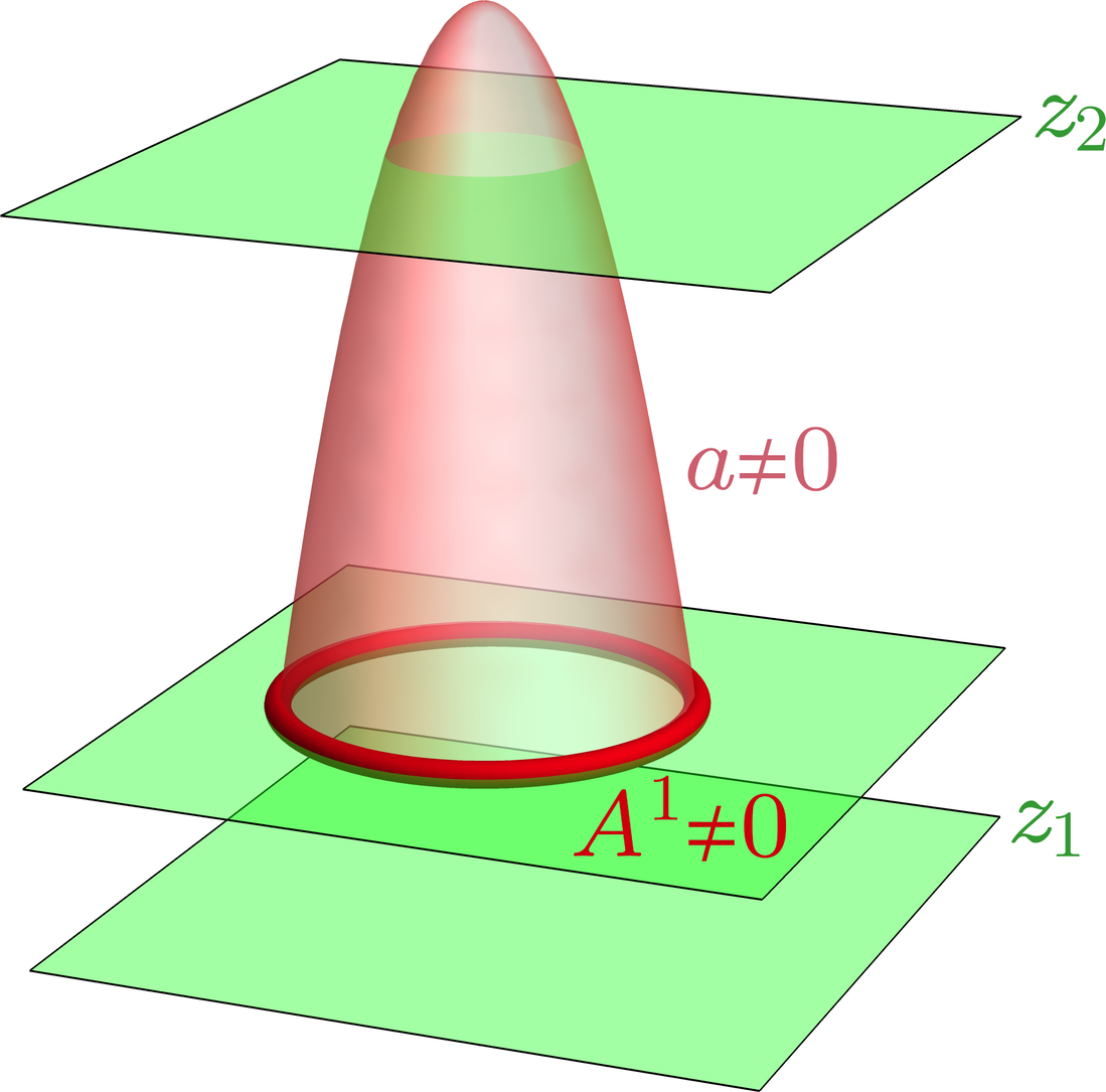
(a)

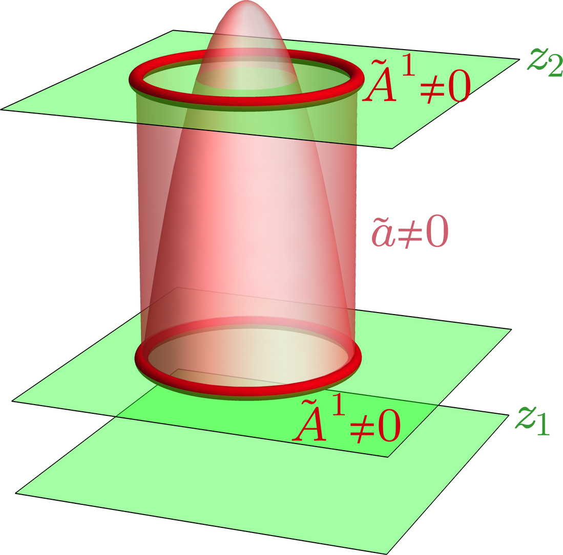
(b)

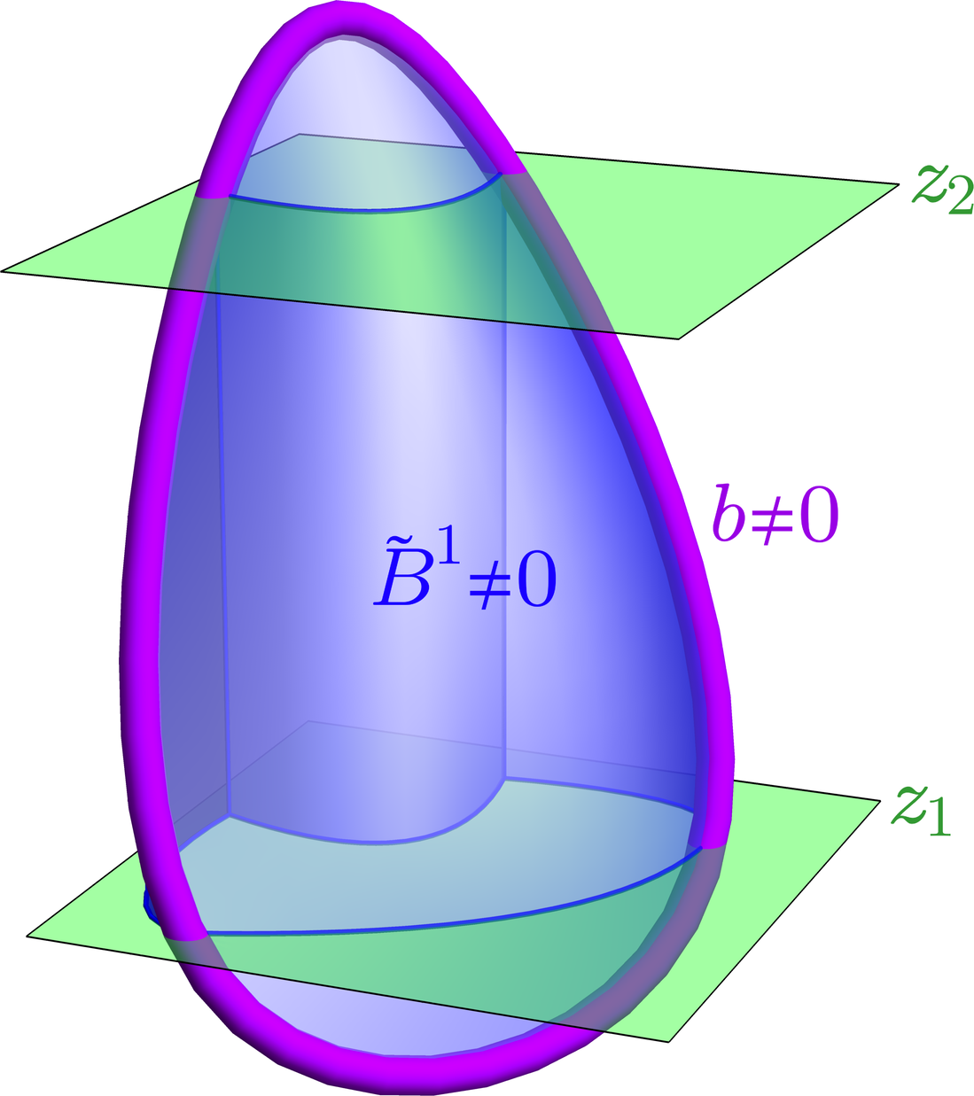
(d)

Figure 4: Examples of how the duality Eq. (13) acts on field configurations that satisfy the equations of motion $da+\sum_{k}m_{k}A^{k}=dA^{k}=db=(dB^{k}+n_{k}b)\wedge e^{k}=0$. Some leaves are shown in green. (a) A membrane of $a\neq 0$ (light red) that ends on a loop of $A^{1}\neq 0$ (red) gets mapped to (b) the same fields but with the membrane extended vertically (from the $A^{1}\neq 0$ loop) to $z_{2}$, ending on a new loop of $\tilde{A}^{1}\neq 0$. $A^{k}=0$ and $a=0$ elsewhere. (c) A membrane of $B^{1}\neq 0$ (light blue) with a boundary on a loop of $b\neq 0$ (purple). (c) is mapped to (d), which adds an additional membrane of $\tilde{B}^{1}\neq 0$ within $z_{1}<z<z_{2}$. Importantly, note that $da+\sum_{k}m_{k}A^{k}=(dB^{1}+n_{1}b)\wedge e^{1}=0$ is satisfied everywhere in (a) and (c) since membranes of $a\neq 0$ and $B^{1}\neq 0$ end on loops of $A^{1}\neq 0$ and $B^{1}\neq 0$; while $d\tilde{a}=d\tilde{B}^{1}\wedge e^{1}=0$ is satisfied for $z_{1}<z<z_{2}$ in (b) and (d) since membranes of $\tilde{a}\neq 0$ and $\tilde{B}^{1}\neq 0$ do not have boundaries in this region.

$\leftrightarrow$   
   $\leftrightarrow$

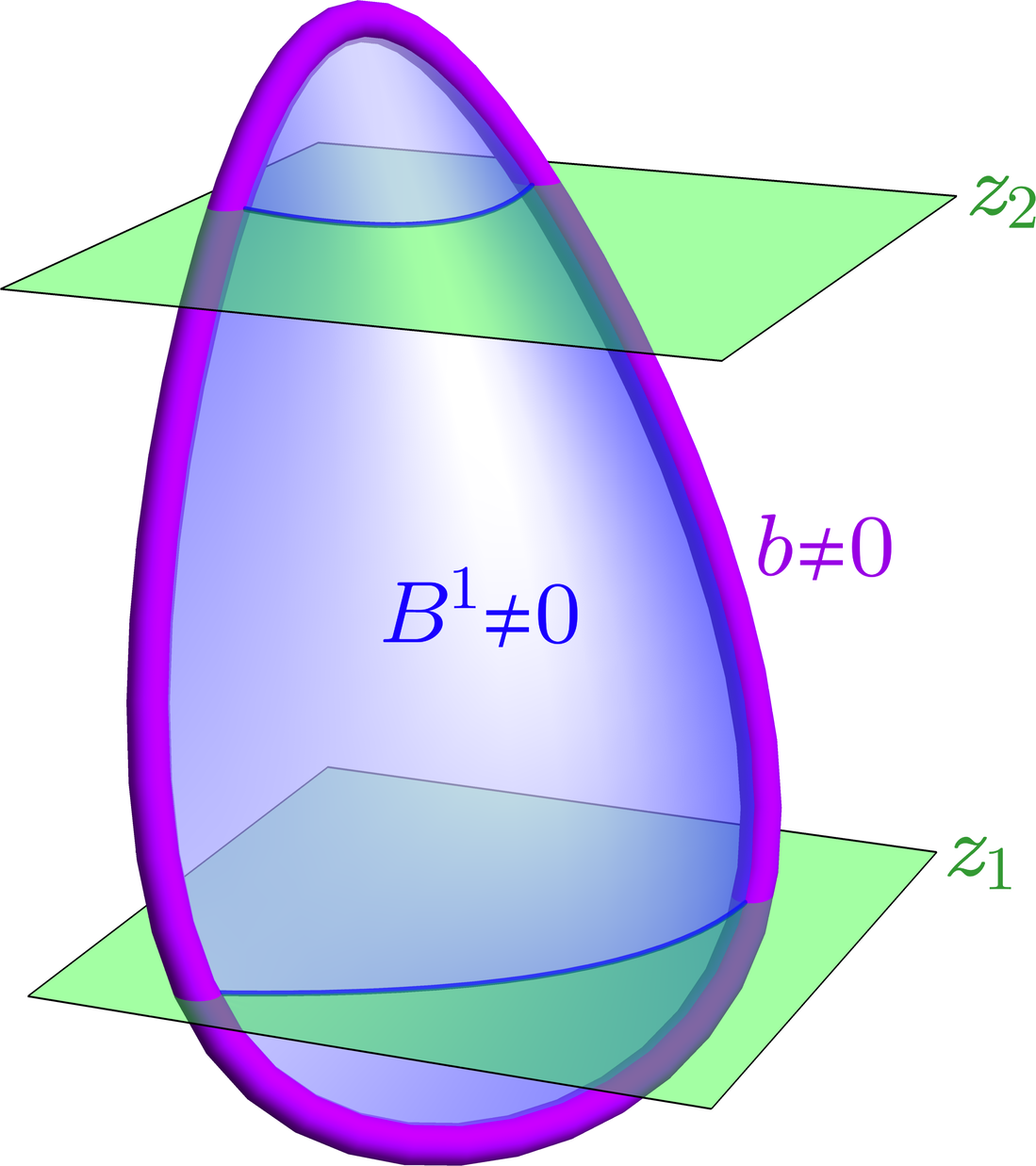
(c)

Ref. Shirley et al. (2018) showed that a finite-depth local unitary transformation can be used to decouple a layer of toric code from the X-cube model and reduce the lattice length of the X-cube model by 1 in one direction [Eq. (47)]. By repeating this process, a stack of many neighboring layers can be exfoliated. This is the analog of the field theory duality that we study here.

On a lattice, removing $L$ neighboring layers requires a local unitary transformation of depth $O(\log\,L)$ [by exfoliating every other layer for $O(\log\,L)$ steps]. As such, removing many layers can not be done using a constant-depth local unitary transformation. The fact that the unitary transformation can not be of constant depth implies that the duality maps some local operators to nonlocal operators.

This nonlocality is made explicit by the integrals in Eq. (13). See also Fig. 4a, which shows an example of how the duality acts on an example field configuration.

The duality can also change the spacetime dimensionality of gauge invariant operators. For example, if $M_{k}=N$, $n_{k}=1$, and $e^{1}=dz$ is the only foliation, then the duality will map:

$$e^{\mathrm{i}\oint_{\partial\mathcal{M}_{2}^{\text{F}}}a\,+\,\mathrm{i}\int_{\mathcal{M}_{2}^{\text{F}}}A^{1}}\leftrightarrow e^{\mathrm{i}\oint_{\partial\mathcal{M}_{2}^{\text{F}}}\tilde{a}}$$ (49)

where $\mathcal{M}_{2}^{\text{F}}$ is a disk within the XZ plane and between $z_{1}<z<z_{2}$, and $\partial\mathcal{M}_{2}^{\text{F}}$ denotes its circular boundary. The left hand side is a gauge invariant 2D membrane operator, which has higher dimension than the 1D string operator on the right hand side. The right hand side is an example of the string operator in Eq. (6) (which is gauge invariant since $\tilde{n}_{k}=0$).

Applying the duality throughout the entire spacetime and to all foliations would appear to result in a duality to an FQFT with $n_{k}=0$, which describes decoupled 3+1D and a foliation of 2+1D BF theories. However, such a mapping would require taking the limit $z_{1}\to-\infty$ and $z_{2}\to+\infty$ in Eq. (13), which would merely push the nontrivial fracton physics out to infinity. Nevertheless, between $z_{1}$ and $z_{2}$, the theory would be a TQFT with no apparent fracton physics remaining in this region.

G.1 Details

Below, we show that the duality transformation in Eq. (13) transforms the equations of motion (33)–(36) by $n_{1}\leftrightarrow\tilde{n}_{1}(z)$ [Eq. (12)]. (We will assume that there are no source terms: $J^{k}=0$, $I^{k}=0$, $j=0$, $i=0$.) Eqs. (34) and (35) do not transform for $z\neq z_{2}$ since $n_{k}$, $a$, and $B^{k}$ do not appear in these equations of motion.

When $z_{1}<z<z_{2}$, Eq. (33) transforms as follows:

$$\quad\;\left\{dB^{1}+n_{1}b\right\}\wedge e^{1}$$ (50)

$$=\left\{d\tilde{B}^{1}+dB^{1}(z_{2})-n_{1}d\int_{z}^{z_{2}}b+n_{1}b\right\}\wedge e^{1}$$ (51)

$$=\left\{d\tilde{B}^{1}+dB^{1}(z_{2})-n_{1}\int_{z}^{z_{2}}(db-dz\wedge\partial_{z}b)+n_{1}b\right\}\wedge e^{1}$$ (52)

$$=\left\{d\tilde{B}^{1}+dB^{1}(z_{2})+n_{1}[b(z_{2})-b]+n_{1}b\right\}\wedge e^{1}$$ (53)

$$=d\tilde{B}^{1}\wedge e^{1}$$ (54)

Eq. (51) results from solving for $B^{1}$ in Eq. (13) and plugging that in. Eq. (52) follows from splitting the exterior derivative into spacetime components: $\left[d\int_{z}^{z_{2}}b\right]\wedge e^{1}=\sum_{\mu=0,1,2}dx^{\mu}\wedge\left[\int_{z}^{z_{2}}\partial_{\mu}b\right]\wedge dz=\left[\int_{z}^{z_{2}}(db-dz\wedge\partial_{z}b)\right]\wedge e^{1}$. Eq. (53) follows from the equation of motion $db=0$ and integrating the total derivative $\partial_{z}b$. Eq. (54) follows from the original equation of motion (33): $dB^{k}+n_{k}b=0$.

When $z_{1}<z<z_{2}$, Eq. (36) transforms as follows:

$$\quad\;da+\sum_{k}m_{k}A^{k}$$ (55)

$$=d\tilde{a}-m_{1}d\int_{z_{1}}^{z}A^{1}+\sum_{k}m_{k}A^{k}$$ (56)

$$=d\tilde{a}-m_{1}\int_{z_{1}}^{z}dA^{1}+\sum_{k\neq 1}m_{k}A^{k}$$ (57)

$$=d\tilde{a}+\sum_{k\neq 1}m_{k}A^{k}$$ (58)

Eq. (56) results from solving for $a_{\mu}$ in Eq. (13) and plugging that in. Eq. (57) follows from splitting the exterior derivative into spacetime components: $d\int_{z_{1}}^{z}A^{1}=dx^{\mu}\wedge\partial_{\mu}\int_{z_{1}}^{z}A^{1}=\sum_{\mu=0,1,2}\int_{z_{1}}^{z}dx^{\mu}\wedge\partial_{\mu}A^{1}+dz\wedge\partial_{z}\int_{z_{1}}^{z}A^{1}=\int_{z_{1}}^{z}dA^{1}+A^{1}$, where the last equality makes use of Eq. (4) and the definition $\big{(}\int_{z_{1}}^{z}A^{1}\big{)}_{\mu}\equiv\int_{z_{1}}^{z}A^{1}_{3\mu}\,dz$ [defined below Eq. (13)]. Eq. (58) follows from the equation of motion (34): $dA^{k}=0$. The $A^{1}\leftrightarrow\tilde{A}^{1}$ transformation in Eq. (13) is necessary so that Eq. (36) remains satisfied at $z=z_{2}$.

For $z<z_{1}$ or $z>z_{2}$, the equations of motion do not transforms since the duality transformation is trivial in this region of spacetime. Therefore, we have shown that the duality transformation (13) transforms the equations of motion (33)–(36) by $n_{1}\leftrightarrow\tilde{n}_{1}(z)$ [Eq. (12)].

Appendix H Connection to Previous Work

Here, we discuss how the FQFT in Eq. (3) is related to the field theory introduced in Ref. Slagle et al. (2019a):

$$\tilde{L}=\frac{N}{2\pi}\left[\sum_{k}B^{k}\wedge d\tilde{A}^{k}\wedge e^{k}+b\wedge da+\sum_{k}b\wedge\tilde{A}^{k}\wedge e^{k}\right]$$ (59)

The above Lagrangian is copied from Eq. (3) of Ref. Slagle et al. (2019a) (up to some minus signs), except we place a tilde on the 1-form $\tilde{A}^{k}$ to differentiate it from the foliated (1+1)-form gauge field $A^{k}$ in this work.

To connect to the FQFT [Eq. (3)], we can make the following hand-wavy replacement in $\tilde{L}$ (and generalize the coefficients):

$$\tilde{A}^{k}\wedge e^{k}\to A^{k}$$ (60)

As mentioned in Sec. 4.1.1 of Ref. Slagle et al. (2019a), it is difficult to quantize the coefficient $N$ in Eq. (59). The reason is that rescaling the foliation $e^{k}\to\gamma e^{k}$ [Eq. (2)] for constant $\gamma$ does not affect the foliation, but it would rescale $N$. By absorbing the foliation field $e^{k}$ into $\tilde{A}$ as in Eq. (60), the foliation field no longer explicitly appears in the Lagrangian. This makes it possible to quantize the coefficients of the FQFT.