On the Value of Oversampling for Deep Learning in Software Defect Prediction

Abstract

One truism of deep learning is that the automatic feature engineering (seen in the first layers of those networks) excuses data scientists from performing tedious manual feature engineering prior to running DL. For the specific case of deep learning for defect prediction, we show that that truism is false. Specifically, when we pre-process data with a novel oversampling technique called fuzzy sampling, as part of a larger pipeline called GHOST (Goal-oriented Hyper-parameter Optimization for Scalable Training), then we can do significantly better than the prior DL state of the art in 14/20 defect data sets. Our approach yields state-of-the-art results significantly faster deep learners. These results present a cogent case for the use of oversampling prior to applying deep learning on software defect prediction datasets.

1 Introduction

Can deep learning (DL) be applied to SE data without first adjusting those learners to the particulars of SE? Many researchers believe so. A common claim is that DL supports a kind of automated feature engineering [1, 2, 3, 4, 5] that lets data scientists avoid tedious manual feature engineering, prior to running their learners.

Figure 1.a F1 scores before (off-the-shelf deep learning)	Figure 1.b F1 scores after (using the methods of this paper)

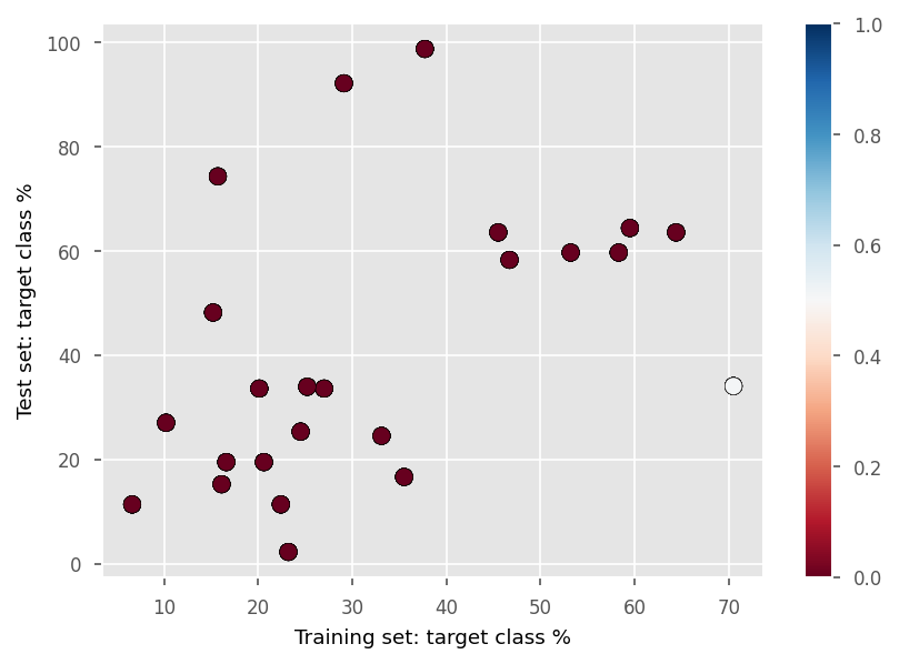
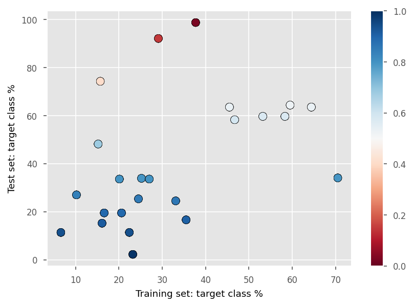
Figure 1: Defect prediction using project data described later in this paper. Data is divided 70:30 into train:test sets. Performance scores come from applying a model (learned from training data) to the test data. In this figure blue dots are good red are bad. Figure 1.a and Figure 1.b were created using the technology described in lines #1 and #8 (respectively) of Table II (described. below). To allow comparison between figures, Figure 1.b shows (i)  the imbalance before applying the methods of this paper and (ii) the Figure 1.b performance scores come after after we applied the methods of this paper.

It is timely to assess such claims. DL is now widely applied to many SE tasks such as bug localization [6], sentiment analysis [7, 8], API mining [9, 10, 11], effort estimation for agile development [12], code similarity detection [13], code clone detection [14], etc. Despite its widespread use, few SE researchers critically examining the utility of deep learning for SE. In their literature review, Li et al. [15] explored over 40 SE papers facilitated by DL models and found that 33 of them used DL without comparison to other (non-DL) techniques. In our own literature review on DL in SE (reported below in §2), we find experimental comparisons of DL-vs-non-DL in less than 10% of papers.

This paper shows that a non-DL technique called “oversampling” (artificially generating members of a minority class prior to running a learner) dramatically improves deep learning. Such resampling is not widespread practice. For example, Wang et al. [16] recently achieved state-of-the-art performance in defect prediction. Their paper did not discuss or deploy any class imbalance techniques–a pattern that repeats across all the papers seen in our literature review. This is a limitation with current research since:

• When we tried their methods using static code attributes we found that (a) many data sets were imbalanced (target classes under 30% or even less) and (b) standard DL performed quite poorly (see all the red dots in Figure 1.a).

• But applying our sampling methods improved performance dramatically (see the blue dots of Figure 1.b).

The rest of this paper discusses deep learning and novel oversampling methods that can improve its performance. Our case study is defect prediction from static code features (e.g. depth of inheritance trees, class coupling and cohesion, lines of code, etc) to guide human inspection effort towards small regions of the code base that are most likely to have errors. Our argument will proceed as follows: we will first build a case for the problems with learning from a class-imbalanced dataset. Then, we will discuss approaches used in the literature for alleviating these problems. In particular, we will discuss the approach studied by Buda et al. [17]. We will then show that for defect prediction, this approach is insufficient, and extend their method to a novel adaptive oversampling approach. We will show that when used as part of a larger framework called GHOST, we achieve state-of-the-art results significantly faster. Our ablation study will demonstrate that the biggest leaps in performance come from our novel oversampling approach, which is the core component of GHOST.

Before starting, we digress to make three points:

• It is important not to overstate our results. This paper only shows that oversampling improves deep learning for defect prediction. That said, the results of this paper motivate a new approach to deep learning where researchers check if those algorithms can be extended and improved by support tools like our adaptive oversampling.

• Any paper recommending oversampling needs to document that it avoids the following threat to validity. While we oversample the training data, we never modify the test data (since that would we mean are not testing on the kinds of data that might be encountered in the field).

• To support open science, all the scripts and data used in this study are freely available online.

2 Background

2.1 Defect Prediction

Every quality assurance decision is associated with a human and resource cost to the developer team. It is impractical and inefficient to distribute equal effort to every component in a software system [18]. Hence, it is common to match the quality assurance (QA) effort to the perceived criticality and bugginess of the code for managing resources efficiently.

Defect prediction models [19] are one way to take a look at the incoming changes and focus inspection effort on specific modules (ignoring others). There is much industrial interest in such predictors: a survey of 395 practitioners from 33 countries and five continents [20] found that over 90% of the respondents were willing to adopt defect prediction techniques. Such predictors can save labor compared with traditional manual methods. For a telecommunications company, Misirli et al. [21] built a defect prediction model that predicted 87% of code defects and decreased inspection efforts by 72% (and reduced post-release defects by 44%). Kim et al. [22] applied a defect prediction model to API development process at Samsung. Their models could predict the bug-prone APIs with reasonable accuracy (0.68 F1 scores) and reduce the resources required for executing test cases. These defect predictors require very simple code features and hence are very cheap to build (compared to using, say, a static code analysis tool with an expensive license) And while these models use simple attributes, they are still remarkably effective. Rahman et al.  [23] compared (a) static code analysis tools FindBugs, Jlint, and PMD with (b) defect predictors (which they called “statistical defect prediction”) built using logistic regression. No significant differences in cost-effectiveness were observed.

2.2 Oversampling

Building classification models for, say, defect prediction becomes complicated [24, 25, 26] when the target class is rare (since it is hard for the learner to build a model that can find that target). To solve that problem, much prior work as argued for oversampling, augmented with some tuning, as a method for improving learner performance.

Buda et al. [17] note that in many cases, simple oversampling suffices; i.e., many times, pick one example at random then add that it several times back into the training set. Other researchers take a different view. Chawla [26] showed that by generating synthetic examples of a scare minority class, it is possible to boost learner performance. In their SMOTE algorithm, examples in the minority class build synthetic examples halfway between themselves and their near neighbors.

Oversampling alleviates class imbalance by drawing additional samples from the minority class. As shown in Figure 1, in datasets with a class imbalance, the performance of the learner drops drastically; only in a case with less severe imbalance (training set imbalance = 70%) does the learner achieve moderate performance. A standard method of doing this is by simply duplicating the points in the minority class until the number of samples in both classes is the same. Oversampling is not the only way to fix the class imbalance problem, however. Another common approach is undersampling, where the majority class is downsampled to match the number of samples in the minority class.

2.3 Oversampling and Tuning

Oversampling algorithms like SMOTE come with various control parameters that have to be set via “engineering judgement” (i.e. guessing). Researchers like Agrawal et al. [24] augment SMOTE with tuning algorithms that automatically find those parameters. There are many such “hyperparameter optimziation” methods such as MOEA/D, NSGA-II, differential evolution, hyperopt, etc [27, 28, 29]. In subsequent work, Agrawal et al. [30] found a measure (that they call “intrinsic dimensionality”) that can be used to select which hyperparameter optimizer works best for different kinds of data. For example, based on their analysis, this paper does not use Hyperopt [29] (since that algorithm tends to overfit on our kind of data). Instead, following Agrawal et al.’s advice, we will use the DODGE [27] hyperparameter optimizer to tune our oversamplers. DODGE experiments with a set of tunings $T_{i}$ in a sequential ordering $T_{1},T_{2}\ldots$ etc. If any tuning $T_{i}$ results in a performance near some prior tuning $T_{j<i}$ then DODGE marks that tuning as “tabu” and avoids any similar tuning. For two reasons, DODGE runs very quickly. Firstly the tabu space grows, this kind of search very quickly runs out of new things to try (hence DODGE can terminate after just a few dozen experiments). Secondly, prior to doing any tuning, Agrawal et al. reduce the feature space using feature selection. Feature selectors prune superfluous attributes (i.e. those not associated with the the target class). Following the advice of Hall and Holmes [31], DODGE uses Hall’s CFS selector [32]. Finally, we found that using SMOTE [26] improved the results of DODGE, so we used it to provide a stronger baseline.

2.4 Deep Learning

Deep learning (DL) is an extension of prior work on neural networks where the adjective “deep” refers to the use of multiple layers in the network. In the 1960s and 1970s it was found that very simple neural nets can be poor classifiers unless they are extended with (a) extra layers between inputs and outputs; and (b) a nonlinear activation function controlling links from inputs to a hidden layer (which can be very wide) to an output layer. Deep learning is a modern variation on the above which is concerned with a potentially unbounded number of layers of bounded size. Last century, most neural networks used the “sigmoid” activation function ($f(x)=\frac{1}{1+e^{-x}}$), which was subpar to other learners in several tasks; it was only when the ReLU (rectified linear unit) activation function $f(x)=\max(0,x)$ was introduced by [3] that their performance increased dramatically, and they rose to popularity. To train a deep learner:

• Forward-propagation finds outputs from the inputs.

• If the weights learned at layer $i$ (which together form the parameters for the model) are represented as $W^{[i]}$ and $b^{[i]}$ respectively, then

  $$a^{[l]} =f(W^{[l]T}a^{[l-1]}+b^{[l]})$$

  $$a^{[0]} =X$$

  $$a^{[L]} =y$$

  where $L$ is the total number of layers.

• Next, a “backpropagation” [34] approach, first defined in 1986, is used to learn the parameters.

• This process is repeated for a certain number of “epochs”, which is typically chosen a priori.

This paper will compare our new oversampling methods against two DL baselines: a standard deep learner (derived from a literature review) and a state-of-the-art DL defect predictor that we take from the recent SE literature.

For the standard deep learner, we use the kind of learners whose architecture would be “reasonably justifiable” to a deep learning expert. To determine “reasonably justifiable”, we used the results of a recent paper published in a top venue (NeurIPS) by Montufar et al. [35], who derive theoretical lower and upper bounds on the number of piecewise linear regions of the decision boundary learned by a deep learner. By maintaining the number of nodes in the hidden layers of the network to be at least as many as the number of inputs (i.e., the dimensionality of the data), Montufar et al. show that the lower bound for the number of piecewise linear regions in the decision boundary is nonzero. We interpret this as, by setting the number of nodes in each hidden layer equal (for simplicity) to the dimensionality of the data, the network must make an effort to separate the two classes (i.e., using a nonzero number of piecewise linear regions). This certainly does not guarantee an optimal boundary, but it does provide a guarantee for a nontrivial decision boundary.

For the state-of-the-art DL, we use the Wang et al. approach [36, 16]. This is a Deep Belief Network (DBN) [37] that learns “semantic” features and then uses classical learners to perform defect prediction. In that approach, for each file in the source code, they extract tokens, disregarding ones that do not affect the semantics of the code, such as variable names. These tokens are vectorized and given unique numbers, forming a vector of integers for each source file. The features learned in this way are used as input to a classical learner, such as Naive Bayes. Note that, like much of the DL literature, Wang et al. assume that their algorithm automates feature selection (so they do not make use of any other feature engineering pre-processor).

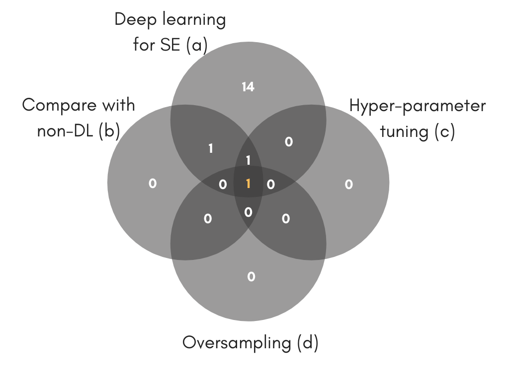
Figure 2: SE+DL literature review. The paper satisfying all three criteria (i.e., $a+b+c$) is [16]; the paper that compares with classical learners (i.e., $a+b$) is [38]. This paper is the only one to satisfy all four criteria, $a+b+c+d$ (denoted by the “1” in the center of this chart).

TABLE I: Selected papers after applying filters (top SE venues, at least 10 cites per year).

Year	Venue	Cites	Use Cases	Title
2016	ICSE	262	defect prediction	Automatically Learning Semantic Features for Defect Prediction [16]
2016	ASE	224	code clone detection	Deep learning code fragments for code clone detection [14]
2015	MSR	183	code representations	Toward Deep Learning Software Repositories [39]
2017	ICSE	83	trace links	Semantically Enhanced Software Traceability Using Deep Learning Technique [8]
2017	ICSME	58	code clone detection	CCLearner: A Deep Learning-Based Clone Detection Approach [40]
2019	TSE	37	story point estimation	A Deep Learning Model for Estimating Story Points [12]
2018	MSR	34	code clone detection	Deep Learning Similarities from Different Representations of Source Code [41]
2017	ICSME	33	vulnerability prediction	Learning to Predict Severity of Software Vulnerability Using Only Vulnerability Description [42]
2018	TSE	24	defect prediction	Deep Semantic Feature Learning for Software Defect Prediction [36]
2017	ICSME	23	duplicate bug retrieval	Towards Accurate Duplicate Bug Retrieval Using Deep Learning Techniques [39]
2019	ICSE	10	bug localization	CRADLE: Cross-Backend Validation to Detect and Localize Bugs in Deep Learning Libraries [43]
2019	MSR	8	defect prediction	DeepJIT: An End-to-End Deep Learning Framework for Just-in-Time Defect Prediction [44]
2019	MSR	5	defect prediction	Lessons Learned from Using a Deep Tree-Based Model for Software Defect Prediction in Practice [38]
2019	ICSE-NIER	4	transfer learning	Leveraging Small Software Engineering Data Sets with Pre-Trained Neural Networks [45]
2018	TSE	4	defect prediction	How Well Do Change Sequences Predict Defects? Sequence Learning from Software Changes [46]
2018	IC SESS	1	language model	A Neural Language Model with a Modified Attention Mechanism for Software Code [47]

2.5 Deep Learning (as seen in SE)

To say the least, much of the technology advocated by this paper is not standard practice in the DL literature. Numerous prominent papers [1, 2, 3, 4, 5] and data science blogs say that DL offers “automated feature engineering” that removes the need for intricate preprocessing. In that view, the first few layers of a deep learning network automatically re-weight/ignore important/irrelevant inputs [3].

Figure 2 summarizes our recent review of DL in SE. Note that very few papers compare their results with non-deep learning methods [16, 38] and none explored oversampling or the hyperparameter tuning methods discussed in §2.3. To build that diagram, using Google Scholar, we search for research papers using the keyword “deep learning AND software engineering”. This returned over 900 papers with at least one citation. To narrow down that list, we looked for papers published in the top venues (defined as per Google Scholar metrics ”software systems”), with $N\geq 10$ cites per year (and for papers more recent than 2017 we used $N\geq 1$). This led to 16 papers listed in Table I.

Outside of the SE literature, we could find one highly cited paper arguing for something like our proposal. Buda et al. [17] show that it is very useful to augment DL with an oversampling preprocessor. According to Google Scholar, this paper has received 731 citations since its publication in 2017. This paper is discussed in the next section.

(Aside: One feature we note from this sample of papers is that the code and data for most of these papers is not always open source. Some are even protected by patent applications. This has implications for reproducibility. For example, this paper baselines some of our results against Wang et al. [16]. Their methods are protected by a patent, and therefore we could not replicate their results using their code. That said, we were able to find their exact training and test sets, which we used for comparison purposes.)

TABLE II: Quartile charts of F1 scores with various treatments. Results are across 240 data points, i.e., 10 repeats, each over the 24 datasets (combined results of the DODGE data and the Wang et al. [16] data). Legend: a = off-shelf deep learning, b = oversampling as studied by Buda et al. [17], c = SMOTE [26], d = fuzzy sampling, e = hyper-parameter tuning.

deep learning oversampling SMOTE fuzzy sampler tuning Median IQR •= median and a b c d e (50th) lines shows IQR #1 ✓ 0 11 #2 ✓ ✓ 0 4 #3 ✓ ✓ ✓ ✓ 0 15 #4 ✓ ✓ ✓ ✓ 0 29 #5 ✓ ✓ ✓ ✓ 51 25 #6 ✓ ✓ ✓ ✓ 51 25 #7 ✓ ✓ ✓ ✓ ✓ 51 25 GHOST = #8 ✓ ✓ ✓ ✓✓ ✓ 80 25

3 Designing our Algorithm (GHOST)

In this section, we describe the components that make up our approach, which we call GHOST. For a detailed statistical analysis of our results, compared to two baselines, see the next section.

Table II shows the relative effectiveness of the components within GHOST. Each row is a different algorithm made up of the components listed in the columns. Several of those components have already been described. For example, deep learning is the “standard deep learner” from §2.3. Also, the SMOTE and tuning components of Table II were discussed above in §2.2 and §2.3. Note that Figure 3(a) and Figure 3(d) came from line #1 and #8 of Table II.

The other components are described in this section. Oversampling is a technique taken from Buda et al. [17]. Also, the fuzzy sampler is a novel method developed for this paper. Note that row #8 has two ticks ✓✓in column d; i.e. in our preferred approach, the fuzzy sampler can be applied twice (see the discussion on line 32 of Algorithm 2, below, for details).

The last two columns of Table II show the median F1 (the harmonic mean of precision and recall) seen across all the data of Table III. Note that, in Table II, “IQR” denotes the (75-25)th interval of F1 scores. In this table, we observe that:

• The first row shows the results presented in Figure 1.a;

• The last row shows the results of Figure 1.b;

• All the other rows show ablation studies where we took out one component from row #8. As can be seen, those ablation studies demonstrated that all the components of row #8 are required to reach our best performance.

The rest of this section discusses the component technologies used in Table II.

TABLE III: Software projects data used in this paper [27]. For an explanation of attributes used in this data, see Table IV.

Project	Train versions	Test versions	Training Buggy %	Test Buggy %
ivy	1.1, 1.4	2.0	22	11
lucene	2.0, 2.2	2.4	53	60
poi	1.5, 2.0, 2.5	3.0	46	65
synapse	1.0, 1.1	1.2	20	34
velocity	1.4, 1.5	1.6	71	34
camel	1.0, 1.2, 1.4	1.6	21	19
jEdit	3.2, 4,0, 4.1, 4.2	4.3	23	2
log4j	1.0, 1.1	1.2	29	92
xalan	2.4, 2.5, 2.6	2.7	38	99
xerces	1.2, 1.3	1.4	16	74

TABLE IV: Static attributes for the classes seen in the Table III data.

Attribute	Description (with respect to a class)
wmc	Weighted methods per class [48]
dit	Depth of inheritance tree [48]
noc	Number of children [48]
cbo	Coupling between objects [48]
rfc	Response for a class [48]
lcom	Lack of cohesion in methods [48]
lcom3	Another lcom metric proposed by Henderson-Sellers [49]
npm	Number of public methods [50]
loc	Number of lines of code [50]
dam	Fraction of private or protected attributes [50]
moa	Number of fields that are user-defined types [50]
mfa	Fraction of accessible methods that are inherited [50]
cam	Cohesion among methods of a class based on parameter list [50]
ic	Inheritance coupling [51]
cbm	Coupling between methods [51]
amc	Average method complexity [51]
ca	Number of classes depending on a class [51]
ce	Number of classes a class depends on [51]
max_cc	Maximum McCabe’s cyclomatic complexity score of methods [52]
avg_cc	Mean of McCabe’s cyclomatic complexity score of methods [52]

Row #1 of Table II shows results from applying the standard DL (of §2.4) to defect prediction. Those results are very low (median of zero), an effect we can explain as follows.

As seen in Table III, there is wide variability in the percent of defects seen in the training and test sets. For example, the defect ratios in velocity’s train:test ratios decrease from 71 to 34%; jEdit’s train:test sets ratios decrease from 23 to 2%; xerces’ train:test sets ratios increase from 16 to 74%. Such massive changes in the target class ratios means that the geometry of the hyperspace boundary between different classifications can alter dramatically between train and test. Therefore, the “appropriate learner” for this kind of data is one that works well for a wide range of ratios of class distributions.

More importantly, we note that in several of these datasets, there is a significant class imbalance problem. From the previous section, our first instinct was to use Buda et al.’s oversampling method to rectify this issue.

Row #2 of Table II shows results from applying the oversampling methods of Buda et al. Specifically, we apply the random oversampling techniques studied by Buda et al. to make the number of samples in the minority class equal to the majority class. In our experiments, we mimic the random oversampling studied by Buda et al. using a common technique, weighted loss functions (see §3.1). This approach, while having the same effect as random oversampling, is significantly computationally cheaper, and therefore, preferred.

As seen in row #2 of Table II, the results from applying the Buda et al. methods are actually worse than Row #1. To explain this negative result, we note that Buda et al. based their conclusions using image, text, and handwriting examples– which is much more complex than the data of Table III where “more complex” can be judged via the number of attributes needed to describe each example:

• Table IV lists 21 attributes for the SE data;

• Buda et al. used image data, which are very high-dimensional.

While the Buda et al. results from row #2 are disappointing, perhaps they are because the particulars of Buda et al’s method was not based on SE data. Hence, in our own experiments, we tested Buda’s intuition (that data sets can be enhanced with oversampling, prior to learning) even though we do not apply their exact methods. This turned out to be a very successful approach since it results in the improvements seen above in Figure 1.

3.0.1 Optimization with DODGE

One key point to observe from those tables is the size of the optimization space.

If each numeric range is divided into five bins using (max-min)/5, and we have 18 options with five choices; i.e. $5^{18}*2^{9}\approx 3*10^{12}$ options.

This space is too large to be exhaustively explored. Hence GHOST and DODGE [27] explore this space heuristically. DODGE’s exploration is defined around a concept called $\epsilon$-domination. Proposed by Deb in 2005 [53], $\epsilon$-domination states that there is little point in optimizing two options if their performance differs by less than some small value $\epsilon$.

DODGE exploits $\epsilon$-domination as follows. $N$ times, repeat: (a) generate configurations at random, favoring those with the lowest weight (initially, all options have a weight $w=1$); (b) if one option generates results within $\epsilon$ of some other, then increase these options’ weights (thus decreasing the odds that they will be explored again). This approach can be a very effective way to explore a large space of options. If we assess a defect predictor on $d=2$ dimensions (e.g. recall and false alarm), the output space of that performance divides into $(1/\epsilon)^{d}$ regions.

3.1 Oversampling, Loss Functions, and Fuzzy Sampling

We now discuss the loss functions we use and our novel oversampling approach (which led to the superior results of line #8 in Table II). In summary, we will apply a fuzzy sampling method to oversample proportional to the class imbalance ratio, in a way to build robust decision boundaries.

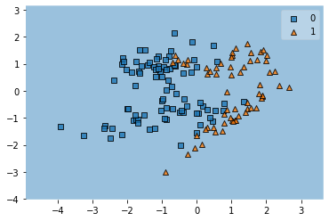
((a)) “Vanilla” network

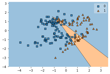
((b)) Weighted loss function

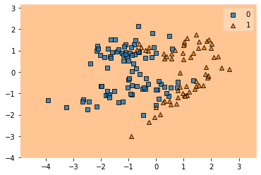
((c)) Weighted loss + fuzzy sampling

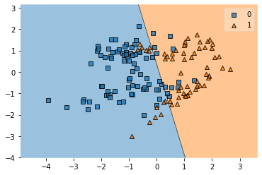
((d)) GHOST

Figure 3: An example of how the different components of the GHOST algorithm work. The background color represents the network’s predictions, while the points represent the true labels. In each figure is the same dataset artificially generated with some noise (orange is the minority class), and the same feedforward architecture (2 layers, 2 units per layer).

In neural networks, the loss function $\mathcal{L}:\mathbb{R}^{n}\times\mathbb{R}^{n}\mapsto\mathbb{R}$ maps the predictions (given the true labels) to a real number, representing how bad the network is. The lower the loss value, the better. The loss is used to calculate the gradients that are used to update the weights of the neural net for the next epoch of learning. Loss can be calculated in various ways but the key point to note here is that, usually, the loss function is fixed prior to learning.

Figure 3 illustrates the effects our various components. To generate this figure, we created an artificial, imbalanced, noisy classification dataset, where the points represent the true labels, 0 and 1. In the figure, class 0 is the majority, with 67% of the samples. Based on the results of Montufar et al. [35], we designed a neural network that can perform well on this dataset, with 2 layers, each with 2 units (we use 2 since there are only 2 inputs).

Figure 3(a) shows the result of running this network on the data. Because the data is imbalanced, and the network is trained on a standard loss function (which assumes the goal is accuracy), the network predicts all points as the majority class–we liken this to a student who finds a workaround to get an easy A in a class, while not truly learning anything.

In Figure 3(b), we use our weighted loss function to mimic Buda et al.’s recommendation. We see that while this helps, it only caters to a slice of the input space that has a majority of the triangles.

In Figure 3(c), we also use our novel oversampling technique–now, we have clearly placed far too much emphasis on the minority class, and the learner scores the easy A by exploiting this.

Our final approach, GHOST, is shown in Figure 3(d). Note how in all the four parts of the figure, the learner (and the data) remains the same; we merely change the preprocessing. Clearly, the preprocessing used has a significant impact on the performance of the deep learner, even with its automated feature engineering.

3.2 Details

We modify the loss function to adapt it to the ratio of classes in the data.

We now elaborate on the weighted loss function. Consider a loss function $\mathcal{L}(y,\hat{y})$ (where $y$ is a vector representing the target outputs, and $\hat{y}$ is a vector representing the predictions) optimized by a neural network. As is the case with defect prediction, consider the case of binary classification. Let $c_{0}$ be the minority class, and $C$ be the set of all classes; for binary classification, this is simply the set $\{c_{0},c_{1}\}$. Denote a training example by a subscript (i.e., let $y_{i}$ denote the target of the $i$th training example), and let $m$ be the number of training examples. Then, the loss function can be rewritten as:

$$\mathcal{L}(y,\hat{y}) =\sum_{i=1}^{m}\mathcal{L}(y_{i},\hat{y_{i}})=\sum_{\begin{subarray}{c}i=1\\ y_{i}=c_{0}\end{subarray}}^{m}\mathcal{L}(y_{i},\hat{y_{i}})+\sum_{\begin{subarray}{c}i=1\\ y_{i}\neq c_{0}\end{subarray}}^{m}\mathcal{L}(y_{i},\hat{y_{i}})$$

We call the above the unweighted loss function. Now, we apply a fairly obvious method of weighting the above as follows: we re-weight the loss function above to:

$$\mathcal{L}^{1}(y_{i},\hat{y_{i}}) =\frac{w_{i}}{n}\sum_{\begin{subarray}{c}i=1\\ y_{i}=c_{0}\end{subarray}}^{m}\mathcal{L}(y_{i},\hat{y_{i}})+\sum_{\begin{subarray}{c}i=1\\ y_{i}\neq c_{0}\end{subarray}}^{m}\mathcal{L}(y_{i},\hat{y_{i}})$$ (1)

where $w_{i}$ is the weight control parameter. For this study, we ran with various weights $w_{i}\in\{1,10,100\}$ and found no appreciable difference between these settings. Hence, in the following, we use $w_{i}=1$. As an aside, we note that this can be extended to multi-class classification.

Clearly, as the minority class shrinks, there is a greater emphasis placed on getting these data points right. This is similar to oversampling by $\frac{w_{i}}{n}$ because with the unweighted loss function and oversampled data, an individual minority class data point (now represented multiple times) contributes more to the loss function than a majority class data point. However, using this weighted loss function has several advantages (a) we do not need to load additional samples into memory (b) we save computation since we do not need to run iterations over these samples (c) it is flexible: we can use a different weight easily.

We certainly are not the first to attempt a reweighted loss function: Ryu et al. [54] used weighted Naive Bayes for cross-company defect prediction. More recently, the weighted Naive Bayes was revisited by Arar et al. [55] for defect prediction. In the AI literature, Lee et al. [56] proposed the use of weighted logistic regression for learning, albeit in the case where some examples are unlabeled (which they consider as negative examples). Lin et al. [57] propose a “focal loss” function that uses an exponential weighting scheme. However, to the best of our knowledge, we are the first to apply this with various weights in the software engineering domain.

3.3 Fuzzy sampling

Our fuzzy sampling triggers on data from the minority classes. When class frequencies alter greatly between the train and the test (as seen in Table III), such points are in danger of fall on the wrong side of the border. Therefore, to protect this from happening, we need to push the decision boundary away.

In describing our approach, we use the following notation:

• we use $f(\textbf{x};\theta)$ to denote a neural network $f(\cdot)$;

• we denote inputs by x;

• the neural network function above is parameterized by the hyperparameter (and preprocessor) set $\theta$;

• we use $\hat{\textbf{y}}$ to denote the predicted values and y to denote the true values;

• we use $\hat{\mathcal{L}}$ to denote our modified loss function

• we use $m$ to denote the number of training samples;

• we use $n$ to represent the fraction of samples belonging to the minority class;

• $\boldsymbol{\Delta r}$ is a user-specified parameter. In our experiments, we used values between 0.01 and 0.05 works well.

• without loss of generality, we use $c_{0}$ to denote the minority class, and $c_{1}$ to denote the majority class;

Using the same notation as the weighted loss functions, let $n$ represent the fraction of samples in the minority class $c_{0}$. Then, iteratively, we add the training samples $(\textbf{x}-i\boldsymbol{\Delta r},c_{0})$ and $(\textbf{x}+i\boldsymbol{\Delta r},c_{0})$ for each sample $(\textbf{x},c_{0})$ in the minority class. At iteration $i$, we add the new samples $\frac{(1/n)}{2^{i}}$ times; we iterate till this value is 0. We choose $\boldsymbol{\Delta}=0.01$, a very small value (to ensure local reasoning). We note here that it might be more beneficial to choose $\Delta r$ based on the statistics of each attribute, but we do not explore that here. Algorithm 1 describes the fuzzy sampling sub-routine

1 for each sample x in the minority class do

2       for $i\in\{0,1,\ldots\}$ such that $\frac{(1/n)}{2^{i}}\geq 1$ do

3             Add $(\textbf{x}\pm i\Delta r,c_{0})$ to the training set $\frac{1/n}{2^{i}}$ times;

4            

5       end for

6      

7 end for

Algorithm 1 Fuzzy sampling

Input : dataset $D$,

performance threshold $\tau=0.5$, twoSample = false

Output : optimal hyper-parameters $\theta^{*}$, performance scores $\boldsymbol{\phi}$

1 Separate $D$ into train and test sets;

2 if twoSample then

3       Apply fuzzy sampling to minority class, reversing the class imbalance;

4      

5 end if

6Apply fuzzy sampling to the training set;

7 Apply SMOTE to the resulting training set;

8 Choose a set of key hyperparameters and pre-processors;

9 Build a list of options for preprocessing and tuning, and assign every node a weight of 0;

10 Sample at random to create random combinations of preprocessors and hyperparameters (number of layers and units per layer);

11 for $N_{1}$ random configurations $\theta_{1},\ldots,\theta_{N_{1}}$ do

12       for $N_{0}$ epochs do

13             $\hat{\textbf{y}}=f(\textbf{x};\theta_{i})$;

14             $\textbf{w}=\textbf{w}-\nabla_{\textbf{w}}\hat{\mathcal{L}}(\textbf{y},\hat{\textbf{y}})$;

15            

16       end for

17      $\phi_{i}=\text{eval}(f)$;

18      

19 end for

20for options that result in metrics with a difference $<\epsilon$ do

21       Reduce the option weight by 1;

22      

23 end for

24forall other options do

25       Increase the weight by 1;

26      

27 end forall

28for $N_{2}$ evaluations do

29       Choose the options $\theta_{i}$ with the highest weight;

30       for $N_{0}$ epochs do

31             $\hat{\textbf{y}}=f(\textbf{x};\theta_{i})$;

32             $\textbf{w}=\textbf{w}-\nabla_{\textbf{w}}\hat{\mathcal{L}}(\textbf{y},\hat{\textbf{y}}$);

33            

34       end for

35      

36 end for

37$\theta^{*}=\text{argmax}_{\theta}\text{eval}(f)$, $\boldsymbol{\phi}=\max\text{eval}(f)$;

38 if $\boldsymbol{\phi}<\tau$ and twoSample = false then

39       Run GHOST with twoSample = true;

40      

41 end if

return $\theta^{*}$

Algorithm 2 GHOST

and Algorithm 2 describes our overall approach:

• Lines 11 to 14 are the deep learner (and here, we use the standard deep learner described above). Based on the results of Theorem 5 of Montufar et al. [35], we use a 2-layer network with 20 units per layer.

• Lines 17 to 22 shows DODGE’s tabu search (discussed in §2.3. The weights of similar results get reduced such that, in subsequent reasoning (see line 24), we do not waste our time sampling from that region.

• Lines 23 to 30 re-runs DL to find good configurations.

• Line 31, 32 say that if we are failing more than half the time $\tau<0.5$ then try again, this time doubling up of the fuzzy sampling.

As pointed out above, Figure 3 contains several components (DODGE, SMOTE, etc). It is hence reasonable to ask if any of those components are superfluous. To check the value of each component, we ran the ablations study shown in Table II. Note that the best results came from using all our components, and the largest increase in performance was realized by adding in fuzzy sampling.

The method of oversampling twice (when twoSample = true) leads to a significantly larger dataset. Specifically, if the original training set contains $m$ minority class samples, and $mk$ majority class samples, i.e., the class imbalance ratio is $k$, then it can be shown that the total number of points when twoSample is true has an upper bound of $7mk+3m$, which is over 3 times as large as the original dataset ($\frac{7mk+3m}{m+km}=3+\frac{4k}{k+1}$. This is important because this increase is also reflected in the runtime of the algorithm. In our testing, we noticed that with twoSample = true, although GHOST is significantly better, it runs 2-3x slower than if it were false, consistent with this result. Therefore, in Algorithm 2, we first run with twoSample = false, and, in line 31, check if our performance is sub-optimal; if so, we run it again with twoSample = true.

3.4 Software engineering and GHOST

In this section, we discuss the applicability of GHOST to software engineering and non-SE tasks, such as image processing.

Because GHOST is fundamentally based on DODGE, we argue that the applicability of GHOST is directly related to the applicability of DODGE. Specifically, because DODGE uses a tabu search mechanism, it is limited to lower-dimensional hyper-parameter spaces. We note that both in the DODGE paper and in our experiments, this condition is met–we tune the preprocessor, the number of layers, and the number of units in each layer, forming a 3-dimensional space. However, in complex domains such as image recognition, this is not possible due to the sophisticated nature of the architectures required to achieve state-of-the-art results. This result has been empirically proven recently by Agrawal et al. [58], who show that DODGE performs poorly in standard AI datasets, such as those found in the UCI repository. For this reason, we discuss our approach only in the context of software engineering (and, in particular, defect prediction), with small hyper-parameter search space dimensionality.

3.5 When not to use GHOST?

With any approach, it is equally important to understand its limitations. In this section, we list two potential pitfalls of using GHOST, and how to fix them in practice.

1. Trespassing: Note that GHOST relies heavily on the use of our novel fuzzy sampling approach, which concentrically adds points around minority samples to push the decision boundary away. In doing so, these newly added samples can inadvertently cross a majority sample, effectively adding more noise to the dataset, and confusing the learner further. If this “trespassing” occurs to many of the minority class samples, it could deteriorate the performance of the learner. This is easily fixable, by using smaller values of $\Delta r$.

2. Balanced datasets: In balanced datasets, fuzzy sampling only adds additional computational overhead in an attempt to balance classes that do not require it. In such cases, we recommend that practitioners simply use hyper-parameter tuning to yield good results.

4 Experiments

The ablation study of Table II was a heuristic method to quickly confirm that no part of our proposed oversampling method is superfluous. That done, we can now explore several research questions, in depth.

RQ1: How well does standard DL perform versus the prior state-of-the-art?

We ask this question since we are critical of SE researchers that merely explore DL without baselining this new method against prior non-DL methods. As we shall see, in such a comparison, standard DL performs poorly.

RQ2: How can we fix DL for defect prediction?

The above discussion around Figure 3 conjectured that (a) widely varying class ratios between train and tests sets introduce instabilities into the boundary between classes; and (b) this problem can be alleviated by oversampling around “at risk” members of the minority classes. To check this conjecture, we apply the system designed above, which resulted in large improvements in DL performance.

RQ3: How scalable is this fixed version of DL?

Any method that tries tuning deep learning (as we do) adds a significant computational burden to an algorithm that is already very slow. Hence it is appropriate to check the scalability of our methods. We show that our methods are scalable since a 400% growth in the size of the data results in a less than 180% growth in the runtimes.

4.1 Experimental Rig

Our experiments compared different defect predictors. For the prior non-DL state-of-the-art we used the methods from DODGE [27] that appeared in a 2019 TSE paper.

For DL, we use a standard deep learner (from §2.4) with 2 layers and 20 units per layer, trained for 30 epochs (these settings were taken from Theorem 5 in Montufar et al. [35]).

For a state-of-the-art deep learner, we used the Wang et al. [36] method from a 2018 TSE paper (also described in §2.4). We use Wang et al. since (a) that paper made a convincing case that this approach represented state-of-the-art results for defect prediction for features extracted from source code and (b) a deep learner is used to extract features, rather than being used as the learner, in contrast to our approach; this forms a valuable comparison.

We also explored two variants of defect prediction:

• Within-project defect prediction (WPDP). Here, models learned from earlier releases of some project predict properties of latter releases of that project.

• Cross-project defect prediction (CPDP). Here, models learned from project1 were then applied to project2.

When comparing against DODGE, we split the data into train and test sets, as shown in Table III. GHOST used the training sets to find good DL settings, which were then applied to the test suite.

As stated above, while we oversample the training data, we never modify the test data (since that would we mean are not testing on the kinds of data that might be encountered in the field).

Because of the stochastic nature of deep learning (caused by random weight initialization), a statistically valid study of its merits should consider the distribution of its performance. For this reason, we run GHOST 20 times for each dataset, for each metric. All the results reported (in Table V and Table VIII) are median values of these 20 runs.

4.2 Data

For this study, we use the same data used in DODGE’s prior study [27] on defect prediction: see Table III. These are all open-source Java projects from the PROMISE repository [59]. Each dataset has 20 static attributes for each software project, described in Table IV.

4.3 Performance Metrics

For this study, we use performance metrics widely used in the defect prediction literature. Specifically, we evaluate the performance of our learners using three metrics: Area Under the ROC Curve (AUC) with the false positive rate on the x-axis and true positive rate on the y-axis, recall, false alarm rate, and popt20. We use these measures to compare against the baseline of Agrawal et al. [27].

• Recall measures the number of positive examples that were correctly classified by a learner.

• The false alarm rate (which we denote by pf) is the fraction of negative samples a classifier incorrectly classifies as a positive example.

• The next metric, popt20 comments on the inspection effort required after a defect predictor is run. To calculate popt20, we list the defective modules before the non-defective modules, sorting both groups in ascending order of lines of code. Charting the percentage of defects that would be recalled if we traverse the code sorted in this manner in the y-axis, we report the value at the 20% point.

• Finally, we report the area under the receiver operating characteristics (ROC) curve (AUC), with false positive rate on the x-axis and true positive rate on the y-axis.

A key benefit of using multiple metrics, aside from a more complete view of the model’s performance, is that it allows us to more concretely test whether deep learning works for all situations. Since some metrics are more important for certain stakeholders (e.g., popt20 comments on the effort needed after the defect predictor are run; others may prefer a combination of high recalls and low false alarm rates, i.e., d2h), this exploration allows us to point out the cases where deep learning may not be the most suitable option.

4.4 Statistics

The statistical methods used in this paper were selected according to the particulars of our experiments.

For example, in the within-project experiments, we are using learners that employ stochastic search. When testing such algorithms, it is standard [60] to repeat those runs 20 times with different random number seeds. Such experiments generate a distribution of 20 results per learner per data set. For those experiments, we use the distribution statistics of §4.4.1 to compare the efficacy of different learners.

For the cross-project experiments, we are comparing our results against the methods of Wang et al. [16], As mentioned in §3, we do not have access to their implementations but we do have access to the train and test sets they use. For these experiments, we must compare our results to the single performance points mentioned in the Wang et al. paper [16]. For those experiments, we use the point statistics of §4.4.2 to compare the efficacy of different learners.

4.4.1 Distribution statistics

Distribution statistics [61, 62] are used to distinguish two distributions of data. In our experimental setup, we run GHOST and DODGE 20 times each, and therefore have a distribution of results for each optimizer. This allows us to use distribution statistical methods to compare results.

Our comparison method of choice is the Scott-Knott test, which was endorsed at TSE’13 [63] and ICSE’15 [62]. The Scott-Knott test is a recursive bi-clustering algorithm that terminates when the difference between the two split groups is insignificant. Scott-Knott searches for split points that maximize the expected value of the difference between the means of the two resulting groups. Specifically, if a group $l$ is split into groups $m$ and $n$, Scott-Knott searches for the split point that maximizes

$$\mathbb{E}[\Delta]=\frac{|m|}{|l|}\left(\mathbb{E}[m]-\mathbb{E}[l]\right)^{2}+\frac{|n|}{|l|}\left(\mathbb{E}[n]-\mathbb{E}[l]\right)^{2}$$

where $|m|$ represents the size of the group $m$.

The result of the Scott-Knott test is ranks assigned to each result set; higher the rank, better the result. Scott-Knott ranks two results the same if the difference between the distributions is insignificant.

4.4.2 Point statistics

For point statistics, we have access to various performance points (e.g. recall) across multiple data sets. To determine if one point is better than another, we have to define a delta $\Delta$ below which we declare two points are the same.

To that end, we use recommendations from Rosenthal [64]. Rosenthal comments that for point statistics, parametric methods have more statistical power (to distinguish groups) than nonparametric methods. Further, within the parametric methods, there are two families of methods: those that use the “$r$” Pearson product moment correlation; and those that use some “$d$” normalized difference between the mean.

After making those theoretical points Rosenthal goes on to remark that neither method is intrinsically better than another. Using Rosenthal’s advice, we apply the most straightforward method endorsed by that research. Specifically, we compare treatment performance differences using Cohen’s delta, which is computed as $\Delta=0.3*\sigma$ where $\sigma$ is the standard deviation of all the values seen across all the data sets. When two methods are different by less than $\Delta$, we say that they perform equivalently. Otherwise, we say that one method out-performs the other if its performance is larger than $\Delta$.

5 Experimental Results

The rest of this paper uses the above methods to explore the research questions listed in the introduction.

5.1 How well does standard DL perform versus the prior state-of-the art? (RQ1)

We are critical of SE researchers that merely explore DL without baselining this new method against prior non-DL state-of-the-art. Accordingly, before we do anything else, we make that comparison.

Table V compares DL versus the prior state-of-the-art (DODGE) versus our preferred new method (GHOST). The wins, ties, and losses from that table are summarized on Table VI. Note that these wins, tie, losses were computed using the statistical methods of §4.4.

As can be seen in the 40 experiments of Table V, DL only performs better than or the same as DODGE in 10/40 experiments (see all the entries marked with “*”). A repeated pattern is that when DL wins on false alarms, it usually does so at the expense of low recalls. Also, when it does achieve a high recall (e.g. for velocity), this usually comes at the cost of high false alarms. Hence we say:

TABLE V: RQ1 and RQ2 results. Cells show medians of 20 runs. Cells with an ”*” show the few cases where DL worked better than DODGE. Dark blue shows top rank (note: for pf, less is better), light blue shows rank two; white shows lowest rank (worst performance). Rankings were calculated via §4.4.1. The train and test versions used here are the same as the DODGE paper (see Table III).

		AUC	popt20	recall	pf
ivy	DL	0.58	0.15	0.33	0.27 *
	DODGE	0.71	0.25	0.85	0.36
	GHOST	0.69	0.31	0.95	0.38
camel	DL	0.55	0.18	0.10	0.04 *
	DODGE	0.58	0.54	0.63	0.36
	GHOST	0.62	0.54	0.65	0.41
jedit	DL	0.61	0.10	0.46	0.16 *
	DODGE	0.63	0.39	0.64	0.25
	GHOST	0.68	0.41	0.91	0.40
log4j	DL	0.55	0.31	0.33	0.13 *
	DODGE	0.61	0.99	0.54	0.22
	GHOST	0.66	0.99	0.75	0.19
velocity	DL	0.50	0.57	0.90 *	0.87
	DODGE	0.61	0.64	0.76	0.47
	GHOST	0.68	0.64	0.82	0.47
synapse	DL	0.54	0.23	0.20	0.05 *
	DODGE	0.65	0.48	0.65	0.23
	GHOST	0.67	0.48	0.63	0.33
lucene	DL	0.58	0.51	0.69 *	0.52
	DODGE	0.61	0.80	0.67	0.36
	GHOST	0.59	0.80	0.7	0.34
xalan	DL	0.55	0.24	0.21	0.09 *
	DODGE	0.71	1.0	0.71	0.14
	GHOST	0.75	1.0	0.76	0.27
xerces	DL	0.52	0.28	0	0.04 *
	DODGE	0.59	0.93	0.54	0.15
	GHOST	0.62	0.94	0.57	0.39
poi	DL	0.61	0.36	0.45	0.18 *
	DODGE	0.72	0.66	0.78	0.22
	GHOST	0.73	0.74	0.78	0.38

TABLE VI: RQ2 results (our DL method vs the prior non-DL state-of-the-art). This table summarizes Table V. The first column indicates the number of wins, ties, and losses for each metric (these are defined using the $\Delta$ measure of Section 4.3 and the directions for “better” defined in Section 4.4. Note that for popt20 and pf, there are multiple ties because both DODGE and GHOST achieve the highest possible score.

	AUC	Recall	popt20	pf	Total
win	7	6	3	2	18
tie	1	3	6	1	11
loss	2	1	1	7	11
win + tie	8	9	9	3	29

Note that these RQ1 results merely show that standard deep learning performs badly. Those results do not explain why that is so. For this task, we must move on to RQ2.

5.2 How to Fix Deep Learning? (RQ2)

The above discussion around Figure 3 showed that (a) widely varying class ratios between train and test sets introduce instabilities into the boundary between classes; and (b) this problem can be alleviated by oversampling around “at risk” members of the minority classes. To check this conjecture, we apply the system designed above.

TABLE VII: RQ2 results. Comparison of GHOST (optimized for recall) with the results of Wang et al. [16], using deep learning-generated “Semantic” features to train a Naive Bayes model on within-project defect prediction. Bold indicates better results, as determined by the point statistics of §4.4.2 (and here, $0.3\sigma=4.91$).

Dataset	Train	Test	Wang et al.			GHOST
			P	R	F1	P	R	F1
synapse	1	1.1	46	66.7	54.4	74.5	98.5	84.6*
	1.1	1.2	57.3	59.3	58.3	66.4	100	79.8*
jEdit	3.2	4	46.7	74.7	57.4	42.3	100	55.9
	4	4.1	54.4	70.9	61.5	74.7	100	85.5*
log4j	1	1.1	67.5	73	70.1	55.6	100	65.9
ivy	1.4	2	21.7	90	35	88.6	100	83.4*
lucene	2	2.2	75.9	56.9	65.1	61.3	100	74.5
	2.2	2.4	66.5	92.1	77.3	60.9	100	75.3
camel	1.2	1.4	96	66.4	78.5	83.4	100	90.9*
	1.4	1.6	26.3	64.9	37.4	26.7	100	38.2
xalan	2.4	2.5	65	54.8	59.5	62.7	100	66
xerces	1.2	1.3	40.3	42	41.1	84.8	100	91.8*
poi	1.5	2.5	76.1	55.2	64	72.2	100	83.2
	2.5	3	81.6	79	80.3	70.2	100	79.7
ant	1.5	1.6	88	95.1	91.4	81.3	93.8	87.1*
	1.6	1.7	98.8	90.1	94.2	52.6	99.4	57.3

TABLE VIII: RQ2 results. Summary of the Table VII GHOST vs Wang et al. results. Comparison of GHOST with the results of Wang et al. [16] on cross-project defect prediction. All results shown are F-1 scores. GHOST results are medians over 20 runs. Bold and dark blue indicates better (in case of tie, both are in bold), as determined by point statistics of §4.4.2 (and here, $0.3\sigma=4.41$).

Source	Target	Wang et al.	GHOST
camel-1.4	jedit-4.1	61.5	47.3
lucene-2.2	log4j-1.1	61.8	51.7
synapse-1.2	ivy-2.0	82.4	30.3
camel-1.4	ant-1.6	97.9	84.9*
xalan-2.5	xerces-1.3	38.6	35.7
jedit-4.1	log4j-1.1	64.5	64.1
log4j-1.1	jedit-4.1	50.3	85.5*
xerces-1.3	ivy-2.0	45.3	94.0*
jedit-4.1	camel-1.4	69.3	90.9*
ivy-2.0	xerces-1.3	42.6	91.8*
lucene-2.2	xalan-2.5	55	65.4
xerces-1.3	xalan-2.5	57.2	66
xalan-2.5	lucene-2.2	59.4	73.8
log4j-1.1	lucene-2.2	69.2	74.6
ivy-2.0	synapse-1.2	43.3	60.9
poi-3.0	synapse-1.2	51.4	58.1
synapse-1.2	poi-3.0	66.1	82.7
ant-1.6	camel-1.4	31.6	36
ant-1.6	poi-3.0	61.9	77.8
poi-3.0	ant-1.6	47.8	62.5

TABLE IX: RQ2 results. Statistical of the Table VII and Table VIII GHOST vs Wang et al. results [16]. Generated using the methods of §4.4.

	WPDP	CPDP	Total
	(Tbl. VII)	(Tbl. VIII)
win	9	14	23
tie	5	2	7
loss	2	4	6
win + tie	14	16	30

Returning to Table V, GHOST can be seen to have more dark blue cells than anything else (i.e. statistically, it is ranked number one most often). Table VI summarizes those results for comparison with DODGE: 18 times, GHOST defeats DODGE (see top-right, Table VI); Tables V and VI display distribution results where algorithms were run multiple times using different random number seeds. Tables VII and VIII, on the other hand, display point distribution results where our algorithms are compared to the single set of performance points reported in prior work.

In Table VII and Table VIII, we show the comparison of GHOST with the results of Wang et al. In these tables, in cases where we used twoSample to improve our results, we denote such results with an asterisk. As shown in the summary (Table IX), we perform as good or better in 14/16 datasets for within-project defect prediction. In cross-project defect prediction, we also note that we win 14/20 times and tie 2/20 times; this suggests that GHOST may be able to generalize well across different projects.

Table IX summarizes the comparison with the results of Wang et al. [16].

These results recommend GHOST over DODGE and DBN. Also, they deprecate the use of off-the-shelf standard DL for defect prediction (since GHOST clearly is preferred to standard DL). We attribute the super performance of GHOST to its weighted loss function.

The exceptions to the above pattern are the GHOST vs DODGE recall results, which we will discuss in the next section. Apart from that, we say that:

5.3 Scalability (RQ3)

TABLE X: Median training time over 20 repeats.

	Training	GHOST
	(secs)	(secs)
ivy	0.78	9m 17s
lucene	0.81	10m 26s
poi	1.09	13m 44s
synapse	0.81	9m 48s
velocity	0.88	10m 20s
camel	1.41	18m 10s
jEdit	1.11	14m 32s
log4j	0.73	8m 29s
xalan	1.61	20m 16s
xerces	1.08	11m 56s

Any method that tries tuning deep learning (as we do) adds a significant computational burden to an algorithm that is already very slow. Hence it is appropriate to check the scalability of our methods.

To address this issue, we report the median training time over 20 runs. The measured time is CPU time, when trained on a 4-core Intel Core i5 CPU. These are summarized in Table X. Clearly, our models are very fast (less than 2 seconds to train on a CPU).

Table X also shows the runtimes for running GHOST on different datasets. Because GHOST runs 20 times to find the median value of a metric, the runtimes we report are for all 20 runs. However, we do not divide this time by 20 as we feel it is scientifically important to run a stochastic experiment multiple times and report statistical results.

Figure 4 shows our scalability results, which we obtain by measuring the training time for different sizes of the datasets. We observe a general trend across all datasets that deep learning scales well with the size of the problem. More specifically, GHOST’s runtimes grow sublinearly. For example, in the xalan results, a 400% increase in data (from a fifth to all the data) leads to a runtime increase of only $2.7/1.5=180\%$.

Hence we say:

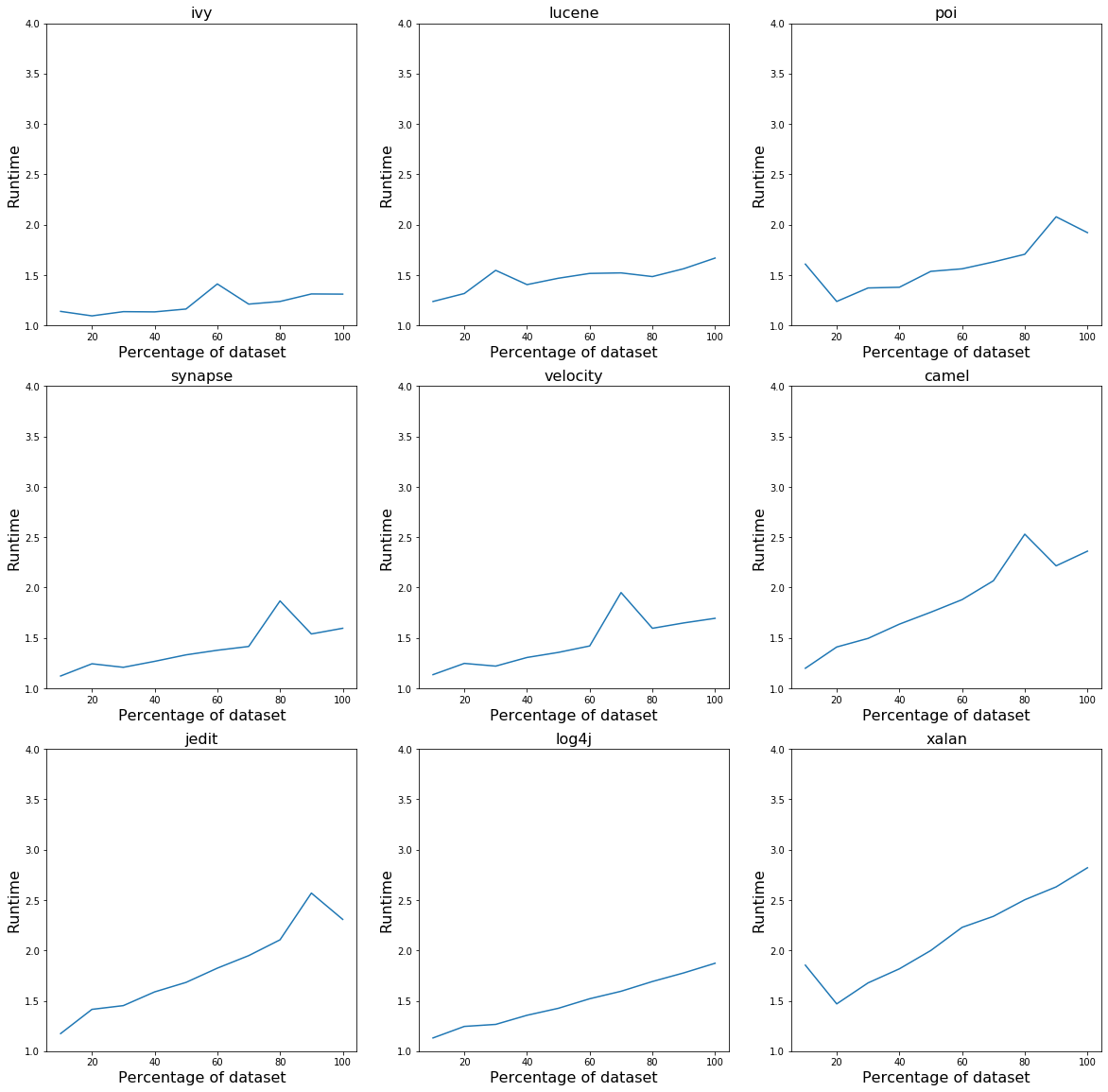
Figure 4: RQ3 results: scalability results for 9 datasets. The x-axis is the perentage of the dataset trained on; the y-axis is the runtime in seconds on a CPU.

6 Threats to Validity

Sampling bias: As with any other data mining paper, it is important to discuss sampling bias. We claim that this is mitigated by testing on 10 SE projects over multiple versions, and demonstrating our results across all of them. Nevertheless, in future work, it would be useful to explore more data.

Learner bias: Our learner bias here corresponds to the choice of architectures we used in our deep learners. As discussed above, we chose the architectures based on our reading of “standard DL” from the literature. That said, different DL architectures could lead to different results.

Evaluation bias: We compared our methods using a range of metrics: AUC, recall, false alarm rate, and popt20. We used these varied evaluation metrics to demonstrate more clearly the benefits of not using learners off-the-shelf, and tuning the loss function optimized. If other performance metrics are used, then other results might be obtained.

Order bias: This refers to a bias in the order in which data elements appear in the training and testing sets. We purposely choose these so that the testing set is from a newer version than the data used in the training set, following the natural order of software releases. Therefore, we argue that such a bias is needed to mimic real-world usage of such learners.

External validity: We tune major hyperparameters using DODGE, removing external biases from the approach. Our baseline results are based on the results of Montufar et al.  [35], which has been evaluated by the deep learning community.

7 Conclusion

There is a discrepancy in the DL literature between those who argue that DL automates feature engineering [1, 2, 3, 4, 5] and the results of Buda et al. [17], which advocate an oversampling pre-processor. To the best of our knowledge, prior to this paper, that discrepancy has not been previously explored using SE data.

We find that:

Through extensive experimentation motivated by both prior work [35] and visualization (see Figure 3), we made a case that class imbalance is a problem for deep learners, and the need for oversampling as a preprocessing step prior to relying on the automated feature engineering offered by deep learning. Our literature review showed that this was lacking in software analytics; our paper is the first to present a cogent, thorough case for (a) comparing against strong, non-DL baselines (b) hyper-parameter tuning for maximum performance of the learners used (c) oversampling to alleviate the class imbalance problem.

Our results showed that while standard random oversampling does not suffice, a novel adaptive version combined with the recommendations of prior work [35, 27, 26] yields state-of-the-art results much faster. The approach we proposed, GHOST, is scalable and works across a wide variety of defect prediction datasets. Further, through ablation studies, we demonstrated the necessity of each component of the algorithm.

Therefore, GHOST can be summarized as a new method that combines deep learning with with two useful extensions: (a) weighted loss functions (see §3.1) (b) a novel fuzzy sampling approach (see §3.3) (c) SMOTE [26]. We demonstrated the efficacy of our approach on 10 defect prediction datasets, using four metrics, as well as on within-project and cross-project defect prediction data as studied by Wang et al. [16]. We compared our results against multiple baselines: (a) a standard deep learner and (b) a prior state-of-the-art result in defect prediction using non-deep learning methods, and (c) a prior state-of-the-art result using deep learning to extract features from code. We presented scalability and runtime tests to demonstrate that deep learners can be trained quickly. We showed that the best results come from learners properly tuned for the dataset and the goal metric (using a weighted loss function).

We note that one could apply the weighted loss functions to classical learners, such as support vector machines (SVMs), which rely on an optimization setup, which has certainly been tried before [54, 55, 56, 57]. However, the ablation studies showed that the most significant improvements to our performance came from our novel fuzzy sampling approach. Moreover, the motivation for fuzzy sampling (i.e., to prevent the boundary from getting too close to the training data) also applies to learners such as decision trees.

We take care to stress that our results relate to defect prediction. As to other areas of software analytics, that is a matter for future search. That said, our results suggest that, for future work, the following research agenda could be insightful:

1. Divided analytics into various domains.

2. Then, for each domain:

   1. Determine the prior non-DL state-of-the-art;

   2. Compare DL with that state-of-the-art;

   3. Seek ways to better adapt DL to that domain.

References

- [1] M. D. Zeiler and R. Fergus, “Visualizing and understanding convolutional networks,” in European conference on computer vision. Springer, 2014, pp. 818–833.
- [2] P. Panda and K. Roy, “Unsupervised regenerative learning of hierarchical features in spiking deep networks for object recognition,” in 2016 International Joint Conference on Neural Networks (IJCNN). IEEE, 2016, pp. 299–306.
- [3] V. Nair and G. E. Hinton, “Rectified linear units improve restricted boltzmann machines,” in Icml, 2010.
- [4] H.-I. Suk, S.-W. Lee, D. Shen, A. D. N. Initiative et al., “Hierarchical feature representation and multimodal fusion with deep learning for ad/mci diagnosis,” NeuroImage, vol. 101, pp. 569–582, 2014.
- [5] R. Yamashita, M. Nishio, R. K. G. Do, and K. Togashi, “Convolutional neural networks: an overview and application in radiology,” Insights into imaging, vol. 9, no. 4, pp. 611–629, 2018.
- [6] X. Huo, F. Thung, M. Li, D. Lo, and S.-T. Shi, “Deep transfer bug localization,” IEEE Transactions on Software Engineering, 2019.
- [7] B. Lin, F. Zampetti, G. Bavota, M. Di Penta, M. Lanza, and R. Oliveto, “Sentiment analysis for software engineering: How far can we go?” in 2018 IEEE/ACM 40th International Conference on Software Engineering (ICSE). IEEE, 2018, pp. 94–104.
- [8] J. Guo, J. Cheng, and J. Cleland-Huang, “Semantically enhanced software traceability using deep learning techniques,” in 2017 IEEE/ACM 39th International Conference on Software Engineering (ICSE). IEEE, 2017, pp. 3–14.
- [9] C. Chen, Z. Xing, Y. Liu, and K. L. X. Ong, “Mining likely analogical apis across third-party libraries via large-scale unsupervised api semantics embedding,” IEEE Transactions on Software Engineering, 2019.
- [10] X. Gu, H. Zhang, D. Zhang, and S. Kim, “Deep api learning,” in Proceedings of the 2016 24th ACM SIGSOFT International Symposium on Foundations of Software Engineering. ACM, 2016, pp. 631–642.
- [11] T. D. Nguyen, A. T. Nguyen, H. D. Phan, and T. N. Nguyen, “Exploring api embedding for api usages and applications,” in 2017 IEEE/ACM 39th International Conference on Software Engineering (ICSE). IEEE, 2017, pp. 438–449.
- [12] M. Choetkiertikul, H. K. Dam, T. Tran, T. T. M. Pham, A. Ghose, and T. Menzies, “A deep learning model for estimating story points,” IEEE Transactions on Software Engineering, 2018.
- [13] G. Zhao and J. Huang, “Deepsim: deep learning code functional similarity,” in Proceedings of the 2018 26th ACM Joint Meeting on European Software Engineering Conference and Symposium on the Foundations of Software Engineering. ACM, 2018, pp. 141–151.
- [14] M. White, M. Tufano, C. Vendome, and D. Poshyvanyk, “Deep learning code fragments for code clone detection,” in Proceedings of the 31st IEEE/ACM International Conference on Automated Software Engineering. ACM, 2016, pp. 87–98.
- [15] X. Li, H. Jiang, Z. Ren, G. Li, and J. Zhang, “Deep learning in software engineering,” arXiv preprint arXiv:1805.04825, 2018.
- [16] S. Wang, T. Liu, and L. Tan, “Automatically learning semantic features for defect prediction,” in 2016 IEEE/ACM 38th International Conference on Software Engineering (ICSE). IEEE, 2016, pp. 297–308.
- [17] M. Buda, A. Maki, and M. A. Mazurowski, “A systematic study of the class imbalance problem in convolutional neural networks,” Neural Networks, vol. 106, pp. 249–259, 2018.
- [18] L. C. Briand, V. Brasili, and C. J. Hetmanski, “Developing interpretable models with optimized set reduction for identifying high-risk software components,” IEEE Transactions on Software Engineering, vol. 19, no. 11, pp. 1028–1044, 1993.
- [19] W. Fu, T. Menzies, and X. Shen, “Tuning for software analytics: Is it really necessary?” Information and Software Technology, vol. 76, pp. 135–146, 2016.
- [20] Z. Wan, X. Xia, A. E. Hassan, D. Lo, J. Yin, and X. Yang, “Perceptions, expectations, and challenges in defect prediction,” IEEE Transactions on Software Engineering, 2018.
- [21] A. T. Misirli, A. Bener, and R. Kale, “Ai-based software defect predictors: Applications and benefits in a case study,” AI Magazine, 2011.
- [22] M. Kim, J. Nam, J. Yeon, S. Choi, and S. Kim, “Remi: defect prediction for efficient api testing,” in Proceedings of the 2015 10th Joint Meeting on Foundations of Software Engineering, 2015, pp. 990–993.
- [23] F. Rahman, S. Khatri, E. T. Barr, and P. Devanbu, “Comparing static bug finders and statistical prediction,” in ICSE. ACM, 2014.
- [24] A. Agrawal and T. Menzies, “Is better data better than better data miners?: on the benefits of tuning smote for defect prediction,” in International Conference on Software Engineering, 2018.
- [25] T. Menzies, A. Dekhtyar, J. Distefano, and J. Greenwald, “Problems with precision: A response to ”comments on ’data mining static code attributes to learn defect predictors’”,” IEEE Transactions on Software Engineering, vol. 33, no. 9, pp. 637–640, 2007.
- [26] N. V. Chawla, K. W. Bowyer, L. O. Hall, and W. P. Kegelmeyer, “Smote: Synthetic minority over-sampling technique,” J. Artif. Int. Res., vol. 16, no. 1, p. 321–357, Jun. 2002.
- [27] A. Agrawal, W. Fu, D. Chen, X. Shen, and T. Menzies, “How to” dodge” complex software analytics,” IEEE Transactions on Software Engineering, 2019.
- [28] J. Bergstra, D. Yamins, and D. D. Cox, “Making a science of model search: Hyperparameter optimization in hundreds of dimensions for vision architectures,” 2013.
- [29] J. Bergstra, R. Bardenet, Y. Bengio, and B. Kégl, “Algorithms for hyper-parameter optimization,” in 25th annual conference on neural information processing systems (NIPS 2011), vol. 24. Neural Information Processing Systems Foundation, 2011.
- [30] A. Agrawal, X. Yang, R. Agrawal, X. Shen, and T. Menzies, “Simpler hyperparameter optimization for software analytics: Why, how, when?” arXiv preprint arXiv:2008.07334, 2020.
- [31] M. A. Hall and G. Holmes, “Benchmarking attribute selection techniques for discrete class data mining,” IEEE Trans. on Knowl. and Data Eng., vol. 15, no. 6, p. 1437–1447, Nov. 2003. [Online]. Available: https://doi.org/10.1109/TKDE.2003.1245283
- [32] M. A. Hall, “Correlation-based feature selection for discrete and numeric class machine learning,” in Proceedings of the Seventeenth International Conference on Machine Learning, ser. ICML ’00. San Francisco, CA, USA: Morgan Kaufmann Publishers Inc., 2000, p. 359–366.
- [33] A. Jacot, F. Gabriel, and C. Hongler, “Neural tangent kernel: Convergence and generalization in neural networks,” arXiv preprint arXiv:1806.07572, 2018.
- [34] D. E. Rumelhart, G. E. Hinton, and R. J. Williams, “Learning representations by back-propagating errors,” nature, vol. 323, no. 6088, pp. 533–536, 1986.
- [35] G. F. Montufar, R. Pascanu, K. Cho, and Y. Bengio, “On the number of linear regions of deep neural networks,” in Advances in neural information processing systems, 2014, pp. 2924–2932.
- [36] S. Wang, T. Liu, J. Nam, and L. Tan, “Deep semantic feature learning for software defect prediction,” IEEE Transactions on Software Engineering, 2018.
- [37] G. E. Hinton, “Deep belief networks,” Scholarpedia, vol. 4, no. 5, p. 5947, 2009.
- [38] H. K. Dam, T. Pham, S. W. Ng, T. Tran, J. Grundy, A. Ghose, T. Kim, and C.-J. Kim, “Lessons learned from using a deep tree-based model for software defect prediction in practice,” in 2019 IEEE/ACM 16th International Conference on Mining Software Repositories (MSR). IEEE, 2019, pp. 46–57.
- [39] J. Deshmukh, S. Podder, S. Sengupta, N. Dubash et al., “Towards accurate duplicate bug retrieval using deep learning techniques,” in 2017 IEEE International conference on software maintenance and evolution (ICSME). IEEE, 2017, pp. 115–124.
- [40] L. Li, H. Feng, W. Zhuang, N. Meng, and B. Ryder, “Cclearner: A deep learning-based clone detection approach,” in 2017 IEEE International Conference on Software Maintenance and Evolution (ICSME). IEEE, 2017, pp. 249–260.
- [41] G. Marcus, “Deep learning: A critical appraisal,” arXiv preprint arXiv:1801.00631, 2018.
- [42] Z. Han, X. Li, Z. Xing, H. Liu, and Z. Feng, “Learning to predict severity of software vulnerability using only vulnerability description,” in 2017 IEEE International Conference on Software Maintenance and Evolution (ICSME). IEEE, 2017, pp. 125–136.
- [43] H. V. Pham, T. Lutellier, W. Qi, and L. Tan, “Cradle: cross-backend validation to detect and localize bugs in deep learning libraries,” in 2019 IEEE/ACM 41st International Conference on Software Engineering (ICSE). IEEE, 2019, pp. 1027–1038.
- [44] T. Hoang, H. K. Dam, Y. Kamei, D. Lo, and N. Ubayashi, “Deepjit: an end-to-end deep learning framework for just-in-time defect prediction,” in 2019 IEEE/ACM 16th International Conference on Mining Software Repositories (MSR). IEEE, 2019, pp. 34–45.
- [45] R. Robbes and A. Janes, “Leveraging small software engineering data sets with pre-trained neural networks,” in 2019 IEEE/ACM 41st International Conference on Software Engineering: New Ideas and Emerging Results (ICSE-NIER). IEEE, 2019, pp. 29–32.
- [46] M. Wen, R. Wu, and S.-C. Cheung, “How well do change sequences predict defects? sequence learning from software changes,” IEEE Transactions on Software Engineering, 2018.
- [47] X. Zhang and K. Ben, “A neural language model with a modified attention mechanism for software code,” in 2018 IEEE 9th International Conference on Software Engineering and Service Science (ICSESS). IEEE, 2018, pp. 232–236.
- [48] S. R. Chidamber and C. F. Kemerer, “A metrics suite for object oriented design,” IEEE Transactions on software engineering, vol. 20, no. 6, pp. 476–493, 1994.
- [49] B. Henderson-Sellers, L. L. Constantine, and I. M. Graham, “Coupling and cohesion (towards a valid metrics suite for object-oriented analysis and design),” Object oriented systems, vol. 3, no. 3, pp. 143–158, 1996.
- [50] J. Bansiya and C. G. Davis, “A hierarchical model for object-oriented design quality assessment,” IEEE Transactions on software engineering, vol. 28, no. 1, pp. 4–17, 2002.
- [51] M.-H. Tang, M.-H. Kao, and M.-H. Chen, “An empirical study on object-oriented metrics,” in Proceedings sixth international software metrics symposium (Cat. No. PR00403). IEEE, 1999, pp. 242–249.
- [52] T. J. McCabe, “A complexity measure,” IEEE Transactions on software Engineering, no. 4, pp. 308–320, 1976.
- [53] K. Deb, M. Mohan, and S. Mishra, “Evaluating the -domination based multi-objective evolutionary algorithm for a quick computation of pareto-optimal solutions,” Evolutionary computation, vol. 13, no. 4, pp. 501–525, 2005.
- [54] D. Ryu and J. Baik, “Effective multi-objective naïve bayes learning for cross-project defect prediction,” Applied Soft Computing, vol. 49, pp. 1062–1077, 2016.
- [55] Ö. F. Arar and K. Ayan, “A feature dependent naive bayes approach and its application to the software defect prediction problem,” Applied Soft Computing, vol. 59, pp. 197–209, 2017.
- [56] W. S. Lee and B. Liu, “Learning with positive and unlabeled examples using weighted logistic regression,” in ICML, vol. 3, 2003, pp. 448–455.
- [57] T.-Y. Lin, P. Goyal, R. Girshick, K. He, and P. Dollár, “Focal loss for dense object detection,” in Proceedings of the IEEE international conference on computer vision, 2017, pp. 2980–2988.
- [58] A. Agrawal and T. Menzies, “Is ai different for se?” arXiv preprint arXiv:1912.04061, 2019.
- [59] J. Sayyad Shirabad and T. Menzies, “The PROMISE Repository of Software Engineering Databases.” School of Information Technology and Engineering, University of Ottawa, Canada, 2005. [Online]. Available: http://promise.site.uottawa.ca/SERepository
- [60] A. Arcuri and L. Briand, “A practical guide for using statistical tests to assess randomized algorithms in software engineering,” in Proceedings of the 33rd International Conference on Software Engineering, ser. ICSE ’11. New York, NY, USA: Association for Computing Machinery, 2011, p. 1–10. [Online]. Available: https://doi.org/10.1145/1985793.1985795
- [61] A. Arcuri and G. Fraser, “Parameter tuning or default values? an empirical investigation in search-based software engineering,” Empirical Software Engineering, 2013.
- [62] B. Ghotra, S. McIntosh, and A. E. Hassan, “Revisiting the impact of classification techniques on the performance of defect prediction models,” in 2015 IEEE/ACM 37th IEEE International Conference on Software Engineering, vol. 1. IEEE, 2015, pp. 789–800.
- [63] N. Mittas and L. Angelis, “Ranking and clustering software cost estimation models through a multiple comparisons algorithm,” IEEE Transactions on software engineering, vol. 39, no. 4, pp. 537–551, 2012.
- [64] R. Rosenthal, H. Cooper, and L. Hedges, “Parametric measures of effect size,” The handbook of research synthesis, vol. 621, no. 2, pp. 231–244, 1994.