Deep Generative Models for Galaxy Image Simulations

Abstract

Image simulations are essential tools for preparing and validating the analysis of current and future wide-field optical surveys. However, the galaxy models used as the basis for these simulations are typically limited to simple parametric light profiles, or use a fairly limited amount of available space-based data. In this work, we propose a methodology based on Deep Generative Models to create complex models of galaxy morphologies that may meet the image simulation needs of upcoming surveys. We address the technical challenges associated with learning this morphology model from noisy and PSF-convolved images by building a hybrid Deep Learning/physical Bayesian hierarchical model for observed images, explicitly accounting for the Point Spread Function and noise properties. The generative model is further made conditional on physical galaxy parameters, to allow for sampling new light profiles from specific galaxy populations. We demonstrate our ability to train and sample from such a model on galaxy postage stamps from the HST/ACS COSMOS survey, and validate the quality of the model using a range of second- and higher-order morphology statistics. Using this set of statistics, we demonstrate significantly more realistic morphologies using these deep generative models compared to conventional parametric models. To help make these generative models practical tools for the community, we introduce GalSim-Hub, a community-driven repository of generative models, and a framework for incorporating generative models within the GalSim image simulation software.

1 Introduction

Image simulations are fundamental tools for the analysis of modern wide-field optical surveys. For example, they play a crucial role in estimating and calibrating systematic biases in weak lensing analyses (e.g., Fenech Conti et al., 2017; Samuroff et al., 2017; Mandelbaum et al., 2018). In preparation for upcoming missions, major collaborations including the Rubin Observatory Legacy Survey of Space and Time (LSST) Dark Energy Science Collaboration (DESC; LSST Dark Energy Science Collaboration, 2012), the Euclid Consortium (Laureijs et al., 2011), and the Roman Space Telescope (Spergel et al., 2015), are currently in the process of generating large scale image simulations of their respective surveys (e.g. Sánchez et al., 2020; Troxel et al., 2019).

Despite the importance of these large simulation campaigns, the most common approach to simulating galaxy light profiles is to rely on simple analytic profiles such as Sérsic profiles (e.g. Kacprzak et al., 2019; Kannawadi et al., 2019). Besides their simplicity, the main motivation for this choice is the existence of prescriptions for the distribution of the parameters of these profiles. These distributions can be directly drawn from observations by fitting these profiles to existing surveys such as COSMOS (Mandelbaum et al., 2012; Griffith et al., 2012), or provided by empirical (Korytov et al., 2019) or Semi-Analytic Models (SAM)s (Somerville & Davé, 2015). These simple models therefore may be used as the basis for fairly realistic image simulations, with galaxies at least matching the correct size and ellipticity distributions as a function of magnitude and redshift.

However, as the precision of modern surveys increases, so does the risk of introducing model biases from these simple assumptions on galaxy light profiles. The impact of model bias for weak lensing shape measurement was for instance explicitly investigated in Mandelbaum et al. (2015), and the impact of galaxy morphologies was measurable, if subdominant, in the calibration of the HSC Y1 shape catalog (Mandelbaum et al., 2018). Beyond their direct effect on shape measurement, assumptions about galaxy light profiles impact various stages of the upstream data reduction pipeline, and in particular the deblending step. It is for instance expected that a majority of galaxies observed by LSST will be blended with their neighbors, given that blending impacts $\sim 60$% of galaxies in the similar wide survey of the Hyper Suprime Cam (HSC; Bosch et al., 2017). As current deblenders, like Scarlet (Melchior et al., 2018), rely on simple assumptions of monotonicity and symmetry of galaxy light profiles, having access to simulations with non-trivial galaxy light profiles will be essential to properly assess systematic deblender-induced biases in number counts, galaxy photometry, and other properties.

Several works have explored galaxy models going beyond simple parametric light profiles. One of the simplest extension is the inclusion of a so-called random knots component (Zhang et al., 2015; Sheldon & Huff, 2017), constituted of point sources randomly distributed along the galaxy light profile, which can model knots of star formation. However, building a realistic prescription for the parameters of this knots component (number of point sources, flux, spatial distribution) is not trivial. In newer large-scale image simulations produced by the LSST DESC (DESC Collaboration, in prep.) a model for this component was obtained by fitting a three component (bulge+disk+knots) light profiles to HST COSMOS image, and then used in image simulations. Similarly, a prescription for how to place these knots based on fitting nearby galaxies was proposed in Plazas et al. (2019). Massey et al. (2004) built a generative model for deep galaxy images based on a shapelet representation, generating new galaxies by perturbing the shapelet decomposition of galaxies fitted in a training set. Finally, image simulations can be based on existing deep imaging, either directly (e.g. Mandelbaum et al., 2012; Mandelbaum et al., 2018), or after denoising (Maturi, 2017) to simulate deeper observations.

With the recent advent of Deep Learning, several works have investigated the use of deep generative models to learn galaxy morphologies. In pioneering work, Regier et al. (2015) proposed the use of Variational AutoEncoders (VAE; Kingma & Welling, 2013) as tools to model galaxy images. The use of VAEs and the first use of Generative Adversarial Networks (GAN; Goodfellow et al., 2014) for astronomical images was further explored in Ravanbakhsh et al. (2017), along with conditional image generation. More recently, Fussell & Moews (2019) demonstrated an application of a StackGan model (Zhang et al., 2016) to generate high-resolution images from the Galaxy Zoo 2 SDSS sample (Willett et al., 2013). Similarly, the generation of large galaxy fields using GANs was demonstrated in Smith & Geach (2019). Beyond generic image simulations, GANs and VAEs have also been proposed to address complex tasks dependent on galaxy morphologies when processing astronomical images, such as deblending (Reiman & Göhre, 2019; Arcelin et al., 2020) or deconvolution (Schawinski et al., 2017). Very recently, Lanusse et al. (2019) proposed to use likelihood-based generative models (e.g. PixelCNN++; Salimans et al. 2017) as priors for solving astronomical inverse problems such as deblending within a physically motivated Bayesian framework.

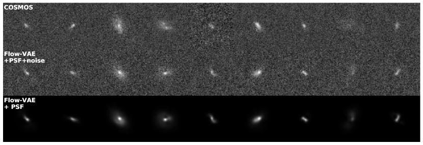
Figure 1: Samples from real COSMOS galaxies (top), and random draws from the generative model (middle) with matching PSF and noise, and conditioned on the size, magnitude, and redshift of the corresponding COSMOS galaxy. The bottom row shows the same generated light-profiles but without observational noise. Because of this conditioning, generated galaxies (middle) are consistent in appearance with the corresponding COSMOS galaxy.

All these precursor works have demonstrated the great potential of Deep Learning techniques, but none of them have gone beyond the stage of simple proof of principle. The goal of this paper is to provide the tools needed to build generative models from astronomical data in practice, i.e., accounting for the instrumental response and observing conditions, as well as providing the software framework to make these tools easily usable by the community as part of the broadly used GalSim image simulation software (Rowe et al., 2015).

To this end, we demonstrate how latent variable models such as GANs and VAEs can be embedded as part of a broader Bayesian hierarchical model, providing a physical model for the Point Spread Function (PSF) and noise properties of individual observations. This view of the problem allows us in principle to learn a denoised and PSF-deconvolved model for galaxy morphology, from data acquired under various observing conditions, and even different instruments. A variety of deep generative models can be used under this framework. As a specific example we propose here a model based on a VAE, complemented by a latent-space normalizing flow (Dinh et al., 2016; Rezende & Mohamed, 2015) to achieve high sample quality. We call this hybrid model a Flow-VAE. We further make our proposed generative model conditional on physical galaxy properties (e.g., magnitude, size, etc) which allows us to sample specific galaxy populations. This is a crucial element to be able to connect image generation to mock galaxy catalogs for generating survey images from a simulated extragalactic object catalog. We train our proposed generative model on a sample of galaxies from the HST/ACS COSMOS survey, and evaluate the realism of the generated images under different morphology statistics that include, but go beyond, the second moments, including size, ellipticity, Gini, M20, and MID statistics (Freeman et al., 2013). Overall, we find excellent agreement between the generated images and real COSMOS images under these statistics and demonstrate that these mock galaxies are quantitatively more complex than simple parametric profiles.

Finally, we introduce GalSim-Hub, a library and repository of trained generative models, interfaced directly into GalSim, with the hope that the availability of such tools will foster the development of generative models of even higher quality, as well as a broader access to these methods by the community. All the tools used to train the generative models presented in this work rely on the Galaxy2Galaxy framework (Lanusse et al, in prep.).

After stating the problem of learning from heterogeneous data in Section 2, we introduce our proposed generative model, dubbed Flow-VAE, in Section 3. We train this model and thoroughly evaluate its performance in Section 4. A summary of our results and future prospects for this work are discussed in Section 5.

2 Learning from corrupted data

While most of the Deep Learning literature on generative models is concerned with natural images (photographic pictures of daily life scenes), learning generative models for galaxy light profiles from astronomical images requires specific technical challenges to be addressed. These include properly dealing with the noise in the observations as well as accounting for the PSF. The question we will focus on in this section is how to learn a noise-free and PSF-deconvolved distribution of galaxy morphologies, from data acquired under varying observing conditions, or even from different instruments. This can be done by complexifying the causal structure of GANs and VAEs, or in other words, integrating these deep generative models as part of a larger Hierarchical Bayesian Model allowing us to cleanly combine these Deep Learning elements within a physically motivated model of the data. In the end, our goal is to produce results like those shown on Figure 1 where the deep generative model only learns galaxy morphologies, while PSF and noise can be added explicitly for a specific instrument or survey. A very similar idea, but for forward modeling multiband photometry instead of images, was proposed in Leistedt et al. (2019). A machine learning component modeling Spectral Energy Distribution (SED) templates was embedded in a larger physical and causal hierarchical model of galaxy photometry, in order to jointly constrain SED templates and photometric redshifts.

2.1 Latent Variable Models as components in larger physically motivated Bayesian networks

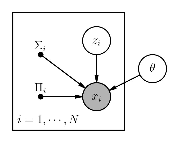
Figure 2: Probabilistic graphical model for observed galaxy images. For each galaxy $i$, the pixel values $x_{i}$ are obtained by transforming an input random variable $z_{i}$ through a parametric generator function $g_{\theta}(z_{i})$ before applying the instrumental PSF $\Pi_{i}$ and adding Gaussian noise with covariance $\Sigma_{i}$.

In this work we consider deep latent variable models (LVM), describing a target distribution $p(x)$ in terms of a latent variable $\bm{z}$ drawn from a prior distribution $p(z)$ and mapped into data space by a parametric function $g_{\theta}$, usually referred to as the generator and taking the form in practice of a deep neural network. While they differ on other points, both VAEs and GANs fall under this class of models. These LVMs can be thought of as flexible parametric models to represent otherwise unknown distributions. As such they can be readily integrated in wider Bayesian networks to fill in parts of the graphical model for which we do not have an explicit formulation.

Let us consider the specific problem of modeling observed galaxy images, with pixel values $\bm{x}$. Making explicit use of our knowledge of the PSF and noise properties of the image, we can model these pixel intensities as being related to the actual galaxy light profile $I$ through:

$$\bm{x}_{i}=\Pi_{i}\ast I_{i}+\bm{n}_{i}\;,$$ (1)

where $\Pi$ represents the PSF (accounting for telescope optics, atmospheric perturbation, and the pixel response of the sensor) and $n$ describes observational noise. In this model, the PSF can typically be estimated from the images of stars in the data itself by the pipeline, or retrieved from a physical optical model of the instrument. Similarly, while the specific noise realization $n$ is unknown, its statistical properties can also be estimated separately from photon-counting expectations or empirical statistics in the imaging. In this work, we will assume a Gaussian noise model, with pixel covariance matrix $\Sigma_{i}$. Note that this covariance can be non-diagonal as the result of the warping of images during data processing. With those two components under control, only the galaxy light profile $I$ remains without a tractable physical model; this is where we can introduce a LVM.

Let us assume that any galaxy light profile $I$ can be realized by a LVM mapping a latent variable $\bm{z}$ into an image through a generator function $I_{i}=g_{\theta}(\bm{z}_{i})$. We can now describe the pixel values of an image as:

$$\bm{x}_{i}=\Pi_{i}\ast g_{\theta}(\bm{z}_{i})+\bm{n}_{i}\;.$$ (2)

Note that while $\bm{x}_{i},\bm{z}_{i},\Pi_{i}.\bm{n}_{i}$ are specific to each observation, the parameters $\theta$ of the LVM are not. A graphical representation of this model is provided in Figure 2.

Learning a model for galaxy morphology now amounts to finding a set of parameters $\theta_{\star}$ for the generator $g_{\theta}$ that ensures that the empirical distribution of the data $p(\bm{x})$ is consistent with the distribution $p_{\theta}(\bm{x})$ described by this Bayesian Hierarchical Model:

$$p_{\theta}(\bm{x})=\prod\limits_{i=1}^{N}\int p_{\theta}(\bm{x}_{i}|\Pi_{i},\Sigma_{i},\bm{z}_{i})p(\bm{z}_{i})\mathrm{d}\bm{z}_{i}\;.$$ (3)

Solving the optimization problem involved in finding the parameters $\theta_{\star}$ is typically a difficult task due to the marginalization over latent variables $\bm{z}$ involved in this expression. Both VAEs and GANs provide tractable solutions, although they differ in methodology: GANs are likelihood-free methods, i.e., they bypass the need to evaluate the marginalized likelihood $p_{\theta}(\bm{x})$ and instead only require the ability to sample from it. On the other hand, VAEs rely on the existence a tractable variational lower bound to the marginalized likelihood.

2.2 Modeling the data likelihood

In this work, we assume the observational noise to be Gaussian distributed, with pixel covariance $\mathbf{\Sigma}$ and 0 mean. This is a common model for sky subtracted images where the noise coming from the dark current and the Poisson fluctuations of the sky background and galaxy can reliably be modeled as Gaussian distributed.

In many situations of interests, $\mathbf{\Sigma}$ is assumed to be diagonal in pixel space and potentially spatially varying. In this case, the likelihood of the data can conveniently be expressed in pixel space as:

$$\log p_{\theta}(\bm{x}_{i}|\Pi_{i},\Sigma_{i},\bm{z}_{i})=-\frac{1}{2}(\bm{x}_{i}-\Pi_{i}\ast g_{\theta}(\bm{z}_{i}))^{t}\mathbf{\Sigma}_{i}^{-1}(\bm{x}_{i}-\Pi_{i}\ast g_{\theta}(\bm{z}_{i}))\\ \ +\ cst\;.$$ (4)

Alternatively, if the noise is known to be correlated but stationary, another tractable assumption is to assume the noise covariance to be diagonal in Fourier space.

$$\log p_{\theta}(\bm{x}_{i}|\Pi_{i},\Sigma_{i},\bm{z}_{i})=\\ -\frac{1}{2}\mathcal{F}\left(\bm{x}_{i}-\Pi_{i}\ast g_{\theta}(\bm{z}_{i})\right)^{t}\mathbf{\Sigma}_{i}^{-1}\mathcal{F}\left(\bm{x}_{i}-\Pi_{i}\ast g_{\theta}(\bm{z}_{i})\right)\ +\ cst\;,$$ (5)

where $\mathcal{F}$ is the forward Fourier transform.

In implicit models such as GANs, evaluating the likelihood is not required; all that is needed is the ability to sample from it. This can be achieved by adding Gaussian noise to the PSF-convolved images created by the generator, before sending them to the discriminator. Note that this step is particularly crucial for GAN generation of noisy images, as there is not enough entropy in the input latent space of the GAN to generate an independent noise realization of the size of an image, needed to match the noise in the data. We find that in practice, without adding noise samples, the generator tries to learn some noise patterns that are actually replicated from image to image.

3 Learning the Generative Model by Variational Inference

In this section, we briefly introduce the various Deep Learning notions underlying the generative models proposed in this work.

3.1 Auto-Encoding Variational Bayes

Figure 3: Schematic representation of a Variational Auto-Encoder. The inference network $q_{\phi}(z|x,y)$ is tasked with predicting the posterior distribution of a given image $x$ and additional information $y$ in latent space $z$. Access to this posterior distribution allows for efficient training of the generative model $p_{\theta}(x|z)$, which models the pixel-level image given the latent variable $z$.

Auto-Encoding Variational Bayes (AEVB), also known as the Variational Auto-Encoder, is a framework introduced in Kingma & Welling (2013) to enable tractable maximum likelihood inference of the parameters of a directed graphical model with continuous latent variables. In such models, one assumes that the observations $\bm{x}$ are generated following a random process involving unobserved latent variables $\bm{z}$ according to some parametric distribution $p_{\bm{\theta}}(\bm{x},\bm{z})=p_{\bm{\theta}}(\bm{x}|\bm{z})p(\bm{z})$, where $\bm{\theta}$ are parameters of this distribution which we aim to adjust so that the marginal distribution $p_{\bm{\theta}}(\bm{x})$ matches closely the empirical distribution of the data. In the context of the model presented in the previous section, these parameters $\bm{\theta}$ will correspond to the weights and biases of the neural network $g_{\theta}$ introduced to model galaxy light profiles.

In this model, we have the freedom to choose any parametric distribution $p_{\bm{\theta}}(\bm{x}|\bm{z})$ to describe the mapping between latent and data space; we only ask for it to be sufficiently flexible to effectively represent the data, and to be easy to sample from. A natural choice is to assume a given parametric likelihood function for the data, and use deep neural networks to learn the mapping from latent space to these distribution parameters. As an example, assuming a Gaussian likelihood for the data, the expression of $p_{\bm{\theta}}(\bm{x}|\bm{z})$ becomes:

$$p_{\bm{\theta}}(\bm{x}|\bm{z})=\mathcal{N}(\mu_{\theta}(\bm{z}),\Sigma_{\theta}(\bm{z}))\;,$$ (6)

where $\mu_{\theta}$ and $\Sigma_{\theta}$ can be deep neural networks depending on a set of parameters $\bm{\theta}$. Training such a model now involves adjusting these parameters as to maximize the marginal likelihood of the model:

$$\hat{\bm{\theta}}=\operatorname*{arg\,max}_{\bm{\theta}}p_{\theta}(\bm{x})=\operatorname*{arg\,max}_{\bm{\theta}}\int p_{\theta}(\bm{x}|\bm{z})p(\bm{z})d\bm{z}\;.$$ (7)

What makes this problem difficult however is that evaluating this marginal likelihood, or its derivatives with respect to the parameters $\bm{\theta}$, is typically intractable analytically and too costly using Monte Carlo techniques.

The idea behind AEVB is to introduce an inference model $q_{\bm{\varphi}}(\bm{z}|\bm{x})$ to estimate for each example $\bm{x}$ the true posterior density $p_{\bm{\theta}}(\bm{z}|\bm{x})$ in the latent space. This model, also known as the recognition model, is performing approximate posterior inference, typically by using a deep neural network to predict the parameters of a parametric distribution (e.g. $q_{\bm{\varphi}}=\mathcal{N}(\mu_{\varphi}(\bm{x}),\sigma^{2}_{\varphi}(\bm{x}))$). This model is essentially replacing a costly MCMC by a single call to a deep neural network to approximate $p_{\bm{\theta}}(\bm{z}|\bm{x})$, this is known as amortized variational inference. The usefulness of this inference model becomes clear when deriving the Kullback-Leibler divergence between this approximation and the true posteriors:

$$\mathbb{D}_{KL}[q_{\phi}(\bm{z}|\bm{x})||p(\bm{z}|\bm{x})] =\mathbb{E}_{q}[\log q(\bm{z}|\bm{x})-\log p(\bm{z}|\bm{x})]$$

$$=\mathbb{E}_{q}[\log q(\bm{z}|\bm{x})-\log p(\bm{z})]+\log p(\bm{x})$$

$$\quad-\mathbb{E}_{q}[\log p(\bm{x}|\bm{z})]$$

$$=\mathbb{D}_{KL}[q_{\phi}(\bm{z}|\bm{x})||p(\bm{z})]+\log p(\bm{x})$$

$$\quad-\mathbb{E}_{q}[\log p(\bm{x}|\bm{z})]\;.$$

Reordering the terms of this expression leads to:

$$\log p(\bm{x})=\mathbb{E}_{q}[\log p_{\bm{\theta}}(\bm{x}|\bm{z})]-\mathbb{D}_{KL}[q_{\phi}(\bm{z}|\bm{x})||p(\bm{z})]\\ +\underbrace{\mathbb{D}_{KL}[q_{\phi}(\bm{z}|\bm{x})||p(\bm{z}|\bm{x})]}_{\geq 0}\;.$$ (8)

Taking into account the fact that the KL divergence is always positive, this leads to the following lower bound on the marginal log likelihood of $x$, known as the Evidence Lower Bound (ELBO):

$$\log p(\bm{x})\geq\mathbb{E}_{z\sim q_{\varphi}(.|x)}[\log p_{\bm{\theta}}(\bm{x}|\bm{z})]-\mathbb{D}_{KL}[q_{\varphi}(\bm{z}|\bm{x})||p(\bm{z})]\;.$$ (9)

Contrary to the original marginal likelihood, the ELBO is now completely tractable, as neither $p(\bm{x})$ or $p(\bm{z}|\bm{x})$ appear in the rhs. The final key element of AEVB is a stochastic gradient descent algorithm (using the so-called reparametrization trick) to efficiently optimize this lower bound in practice (Kingma & Welling, 2013).

This combination of a recognition and generative model, illustrated by Figure 3, is reminiscent of traditional auto-encoders, which follow the same idea of compressing the information down to a latent space and reconstructing the input signal from this low dimensional representation. The difference comes from the second term in the ELBO in Eq. (9) which prevents the latent space representation of particular examples from collapsing to a delta function, and instead promotes the representation learned by the model to stay close to the specified prior $p(\bm{z})$.

Despite the satisfying mathematical motivation for the VAE, it is known that this model usually leads to overly smooth images. The reasons for this problem are an active field of research in machine learning, but are likely due to the difficulty of performing accurate amortized inference of the posterior while training the generator (Kingma et al., 2016; Cremer et al., 2018; He et al., 2019). In this work, instead of trying to address the sub-optimalities of the variational inference, we follow a different direction, originally proposed in Engel et al. (2017), which is to relax the KL divergence term in Eq. (9), and introducing a second model for modeling the latent space aggregate posterior.

3.2 VAE with free bits

Empirically, it is known that training a VAE will tend to find a solution that conforms to the prior $p(\bm{z})$ at the expense of reconstruction and sample quality, leading to over-regularized solutions. A number of different approaches have been proposed to force the model towards better optimization minima (Sønderby et al., 2016), in particular the idea of starting the optimization without the KL divergence term in the ELBO and slowly increasing its strength during training. Rather than relying on an annealing scheme, Kingma et al. (2016) proposed to allow for some amount of information to be communicated through the bottleneck of the auto-encoder without being penalized by the KL divergence:

$$\mathcal{L}_{\lambda}=\mathbb{E}_{z\sim q_{\varphi}(.|x)}[\log p_{\bm{\theta}}(\bm{x}|\bm{z})]-\max\left(\lambda,\ \mathbb{D}_{KL}[q_{\varphi}(\bm{z}|\bm{x})||p(\bm{z})]\right)\;.$$ (10)

The $\lambda$ parameter controls how many free bits of information can be used by the model before incurring an actual penalty. Allowing for more free bits leads to better reconstruction quality as more information about the input image is being transferred to the generator, but allowing for too many free bits essentially removes the regularization of the latent space and we recover a conventional autoencoder, from which we cannot directly sample as the aggregated posterior no longer has any incentive to follow the prior.

The approach proposed in Engel et al. (2017) is to significantly down-weight the KL divergence term in the ELBO, so as to emphasize reconstruction quality first and foremost, at the cost of less regularization in the latent space. Images sampled from this model with Gaussian prior appear significantly distorted and usually meaningless. As a solution to that problem, the authors propose to learn a separate model that models a so-called realism constraint, essentially learning to sample from the aggregate posterior of the data as opposed to the prior. This approach leads to both sharp images and high quality samples, on par with different methods such as GANs can generate. An additional benefit of this approach is that the VAE can be trained once, while the actual posterior sampling model can always be refined later and even made conditional, without needing to retrain the entire auto-encoder (which is in general more costly).

We follow a similar approach in this work, reducing the latent space regularization of the VAE by using the ELBO with free bits loss function defined in Eq. (10). In the next section we will introduce a second latent space model to learn how to sample realistic images.

3.3 Flow-VAE: Learning the VAE posterior distribution

The quality of VAE samples depends strongly on how successful the model is at matching the aggregate posterior distribution of the data to the prior. If this posterior departs from the prior, sampling from the prior will not lead to good quality samples matching the data distribution of the training set. Such failures in matching the posterior to prior may naturally arise in VAEs when the latent space regularization is weaker than the data fidelity term. Another common situation is when training a Conditional VAE, where the model is incentivized to decorrelate the latent variables from the conditional variables (e.g. Ravanbakhsh et al., 2017). This is never perfect, and again the data posterior never completely matches the Gaussian prior and usually exhibits some residual correlations with the conditional variables.

To alleviate these issues, a solution is to train an additional latent space model to learn the aggregate posterior of the data for a given trained VAE. This model can also be made conditional so that it can allow to sample conditionally the latent variables. This two-step process has the advantage of decoupling the training of the VAE on actual images, which can be costly, from the training of the latent-space sampling model, which is much typically much faster. This means for instance that once a VAE is trained, it is possible to inexpensively build a number of conditional models, simply by training different conditional sampling models.

While Engel et al. (2017) proposed to use a GAN to model the latent space, we adopt instead a normalizing flow, a type of Neural Density Estimation method with exact log likelihood, which achieves state-of-the-art results in density estimation while being significantly more stable than GANs. Furthermore, normalizing flows are not susceptible to mode collapse (e.g. Salimans et al., 2016; Che et al., 2016), a common failure mode of GANs which translates into a lack of variety in generated samples. Normalizing flows model a target distribution in terms of a parametric bijective mapping $g_{\theta}$ from a prior distribution $p(\bm{z})$ to the target distribution $p(\bm{x})$. Under this model, the probability of a sample $\bm{x}$ from the data set can be computed by applying a change of variable formula:

$$p_{\theta}(\bm{x})=p(\bm{z})\left|\frac{\partial g_{\theta}}{\partial\bm{z}}\right|(\bm{z})\quad\mbox{ with }\bm{z}=g_{\theta}^{-1}(\bm{x})\;.$$ (11)

With this explicit expression for the likelihood of a data sample under the model, fitting the normalizing flow can be done by minimizing the negative log likelihood of the data:

$$\mathcal{L}=-\log p_{\theta}(\bm{x})=-\log p(\bm{z})-\log\left|\frac{\partial g_{\theta}}{\partial\bm{z}}\right|(\bm{z})\;.$$ (12)

Under the assumption that $\mathbb{D}_{KL}(p||p_{\theta})=0$ is actually attainable (i.e., that $p_{\theta}$, and hence $g_{\theta}$, is flexible enough), it will be achieved at the minimum of this loss function.

The main practical challenge in building normalizing flows is in designing a mapping $g_{\theta}$ that needs to be both bijective, and with a tractable Jacobian determinant. One such possible efficient design is the Masked Autoregressive Flow (MAF) introduced in Papamakarios et al. (2017). A MAF layer is defined by the following mapping:

$$g_{\theta}(\bm{x})=\sigma_{\theta}(\bm{x})\odot\bm{x}+\mu_{\theta}(\bm{x})\;,$$ (13)

where $\odot$ is the Hadamard product (element-wise multiplication), and $\sigma_{\theta}$ and $\mu_{\theta}$ are autoregressive functions, i.e. the $i$th dimension of the output $[\mu_{\theta}(x_{1},\ldots,x_{N})]_{i}$ only depends on the previous dimensions $(x_{1},\ldots,x_{i-1})$. These autoregressive functions are implemented in practice using a masked dense neural network, as proposed in Germain et al. (2015). Given the autoregressive nature of this mapping, its Jacobian takes on a simple lower triangular structure, which makes computing its determinant simple:

$$\log\left|\frac{\partial g_{\theta}(\bm{x})}{\partial\bm{x}}\right|=\sum_{i=0}^{N}\log\sigma_{\theta,i}(\bm{x})\;.$$ (14)

While a single layer of a MAF cannot model very complex mappings, more expressive models can be obtained by chaining several flow layers:

$$g_{\theta}(\bm{x})=f_{\theta}^{0}\circ f_{\theta}^{1}\circ\ldots\circ f_{\theta}^{N}(\bm{x})\;.$$ (15)

In this work, we further extend the baseline MAF model to build a conditional density estimator $p_{\theta}(\bm{x}|\bm{y})$. This can be achieved by providing the conditional variable as an input of the shift and scaling functions $\sigma_{\theta}$ and $\mu_{\theta}$ so that $z_{i}=f(\bm{y},x_{0},\ldots,x_{i-1})$. The resulting conditional density estimator can be used to learn the latent aggregate posterior of the VAE, conditioned on particular parameters of interest, for instance galaxy size or brightness.

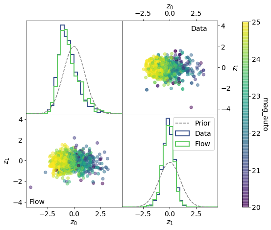
Figure 4: Illustration of latent variable $\mathbf{z}$ distribution as a function of galaxy size for auto-encoded galaxies (top right) and samples from the latent normalizing flow (bottom left). As can be seen from the upper corner plot, the 2d histograms of the latent variables for auto-encoded galaxies can significantly depart from the assumed isotropic Gaussian prior (dashed grey lines) used during training of the VAE. We can also see strong correlations between latent variables z and properties such the magnitude. Both of these effects, i.e. departures from Gaussianity and magnitude-dependence are successfully modeled by the latent normalizing flow in the bottom corner plots.

The upper right corner of Figure 4 illustrates the first two dimensions of the empirical aggregate posterior distribution of a VAE with a 16-d latent space (detailed in Section 4.2). The color indicates the i-band magnitude of the galaxy corresponding to each encoded point. As can be seen from this example, not only is the posterior distribution significantly non-Gaussian, it also exhibits a clear and non-trivial dependence on the galaxy magnitude. The bottom left part of Figure 4 illustrates samples from a conditional normalizing flow which not only reproduces correctly the overall posterior distribution, but also captures the correct dependency on magnitude.

4 Generative Model trained on COSMOS

In this section we present our reference model for the GalSim COSMOS sample using the Flow-VAE approach introduced above.

4.1 The GalSim COSMOS Sample

Our training set is based on the COSMOS HST Advanced Camera for Surveys (ACS) field (Koekemoer et al., 2007; Scoville et al., 2007a, b), a 1.64 deg² contiguous survey acquired with the ACS Wide Field Channel, through the F814W filter (“Broad I”). Based on this survey, a dataset of deblended galaxy postage stamps (Leauthaud et al., 2007; Mandelbaum et al., 2012) was compiled as part of the GREAT3 challenge (Mandelbaum et al., 2014), and forms the basis for our training set. The processing steps and selection criteria required to build this sample are introduced in Mandelbaum et al. (2012) and we direct the interested reader to the Real Galaxy Dataset appendix of Mandelbaum et al. (2014) for a comprehensive description of this sample. We use the deep F814W$<25.2$ version of the dataset, provided with the GalSim simulation software (Rowe et al., 2015) through the COSMOSCatalog class, which provides in addition for each postage stamps the HST PSF, the noise power spectrum, and a set of galaxy properties (e.g., size, magnitude, photometric redshift). As discussed further in the next section, among these additional parameters, we will in particular make use of the Source Extractor F814W magnitude mag_auto, the (PSF-deconvolved) half-light radius hlr, and photometric redshift zphot fields. Applying the default quality cut of exclusion_level=’marginal’ with the COSMOSCatalog leaves us with a sample of 81,500 galaxy postage stamps, which we divide into training and testing sets containing 80,000 and 1,500 galaxies, respectively.

For training, we draw these galaxies at the original 0.03^′′/pix resolution of the coadded images, on postage stamps of size $128\times 128$, convolved with their original PSF and using noise padding. For each galaxy, we also store an image of the associated PSF and noise power spectrum. An illustration of these postage stamps is provided on the top row of Figure 1.

4.2 Generative model

4.2.1 VAE Architecture and Training

For the VAE, we adopt a deep ResNet architecture, based on seven stages of downsampling, with each stage composed on two residual blocs. The depth after a first channel-wise dense embedding layer is set to 16, and is multiplied by two at each downsampling step until reaching a maximum depth of 512. After these purely convolutional layers, we compress the latent representation down to a vector of 16 dimensions using a single dense layer, outputting the mean and standard deviation for a mean-field Gaussian posterior model $q_{\phi}(z|x)$. Likewise, the 16-d latent representation is decoded back to the input dimension of the convolutional generator using a single dense layer. The rest of the generative model is mirroring the architecture of the encoder. At the final layer of the generator, we apply a softplus activation function to ensure the positivity of the light profile generated by the model.

As explained in Section 2, the output of the VAE is then convolved with the known PSF of the input image, and the likelihood that enters the ELBO in Equation 9 is computed using the known noise covariance. The results presented here are obtained using a diagonal approximation to the covariance (i.e. using Equation 4) as it is simpler than a non-diagonal covariance and yields very comparable results. In order to very slightly regularize the pre-convolved light profile generated by the VAE and prevent non-physical very high frequency we include in the loss function, in addition to the ELBO, a small Total Variation (TV) term that penalizes these potential high frequency artifacts which are not otherwise constrained by the data. We add this TV term to the loss with a factor 0.01, which makes it very subdominant to the rest of the loss function.

In addition, in order to provide the encoder network with all the information it needs to learn a deconvolved galaxy image, we feed it an image of the PSF for each example, in addition to galaxy image presented at the input. Without this additional information, the model wouldn’t be able to perform the desired inference task.

Table 1: Hyper-parameters used to train the VAE model.

Parameter	Value
Architecture choices
Number of ResNet blocks	7 (for each encoder/decoder)
Input depth	16
Maximum depth	512
Bottleneck size	16
Optimizer and Training
Optimizer	Adafactor
Number of iterations	125,000
Base learning rate	0.001
Learning schedule	square root decay
Batch size	64
Free-bits	4
Total Variation factor	0.01

Training of the model is performed using Adafactor (Shazeer & Stern, 2018), a variant of the popular ADAM optimizer (Kingma & Ba, 2015) with an adaptive learning rate, with parameters described in Table 1. Note that to make training of this deep encoder/decoder model more efficient, we use the following two strategies:

• Similarly to a UNet (Ronneberger et al., 2015), we allow for transverse connections between corresponding stages of the encoder/decoder during training. Concretely, a random sub-sample of the feature maps at a given level of the generator are simply duplicated from the encoder to the decoder, thus short-circuiting part of the model. This allows the last layers of the generator to start training, even though the deeper layers are not correctly trained yet. This fraction of random duplication of the encoder feature maps to the decoder is slowly decreased during training, until these transverse connections are fully removed.

• To help the dense bottleneck layers to learn a mapping close to the identity, we add an $\ell_{2}$ penalty between inputs and outputs of the bottleneck. The strength of this penalty is again slowly decreased during training.

4.2.2 Latent Normalizing Flow training

Once the auto-encoder is trained, we reuse the encoder with fixed weights to generate samples from the aggregate posterior of the training set images. These samples of the latent space variable $\mathbf{z}$ are in turn used to train the latent space Normalizing Flow described in Section 3.3. This model relies on 8 layers of MAF stages, each of these stages is using two masked dense layers of size 256. Between MAF stages, we alternate between performing a random shuffling of all dimensions and reversing the order of the tensor dimensions, so as to facilitate the mixing between dimensions. Each of the MAF stages is using both shift and scale operations. To help improve the stability of the model during training, we further apply clipping to the output scaling coefficients $\sigma_{\theta}(x)$ generated by each MAF layers. To improve conditional modeling, the additional features $\bm{y}$ are standardized by removing their means and scaling their standard deviation to one.

Training is performed with the ADAM optimizer over 50,000 iterations with a base learning rate of 0.001, following a root square decay with number of iterations.

The trained model is available on GalSim-Hub under the model name “hub:Lanusse2020”. We direct the interested reader to Appendix A for an example of how to use this model with GalSim.

4.3 Auto-Encoding Verification

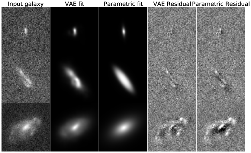
Figure 5: Reconstruction of input images (first column) by the VAE (second column) and by Parametric fit (third column). Residuals for both VAE and parametric models are shown on fourth and fifth columns respectively. From top to bottom are illustrated representative objects of increasing size; smaller compact objects (top) are accurately reconstructed by the model, while larger galaxies exhibit some modeling residuals (bottom). Note that the VAE models are always more complex than their parametric counterparts.

Before testing the quality of the full generative model, we first assess the representation power of the VAE model on galaxies from the testing set. Figure 5 is illustrating how galaxies of different sizes are auto-encoded by the VAE model, compared to a conventional parametric fit to these light profiles (described in the next section). As can be seen, smaller galaxies are very well modeled by the auto-encoder, but for larger galaxies, the model exhibits smoother light profiles, illustrating one of the limitations of such an autoencoder model. The free bits of information used during training of the VAE are intended to mitigate that effect, but are only partially successful. We note furthermore that these large galaxies are under-represented in the training sample, meaning that the model is comparatively less incentivized to correctly model these bright and large galaxies compared to smaller and fainter objects. Accounting and compensating for this training set imbalance could be an avenue to alleviate this effect, but at the price of changing the galaxy distribution being modeled by the VAE.

In all cases, we see on the two rightmost columns of Figure 5 that VAE residuals are significantly smaller than the residuals of the best parametric fit, indicating a better modeling. It is also worth highlighting that in the VAE case, these fitted light profiles are parameterized by only 16 numbers obtained in a single pass of amortized inference, and yet yield more accurate results than the iterative parametric fitting.

4.4 Sample generation validation

In this section, we quantitatively assess the quality of the light profiles generated by our models in terms of several summary statistics, including second order moments and morphological image statistics specifically designed to identify non-smooth and non-monotonic light profiles (Freeman et al., 2013).

To perform these comparisons, we generate three different samples:

• COSMOS sample: Real HST COSMOS galaxies, drawn from the GalSim real galaxy sample.

• Parametric sample: Parametric galaxies drawn from the GalSim best parametric model of real COSMOS galaxies, either single Sérsic or a Bulge+Disk model depending on the best fitting model.

• Mock sample: Artificial galaxies drawn from the generative model, conditioned on the magnitude, size, and redshift of real COSMOS galaxies.

Each tuple of galaxies from these three sets is drawn with the same PSF and matching noise properties as to allow direct comparison.

4.4.1 Second-order moments

We first evaluate the quality of the model in terms of second-order moments of the light profile, defined as:

$$Q_{i,j}=\frac{\int\mathrm{d}^{2}xI(x)W(x)x_{i}x_{j}}{\int\mathrm{d}^{2}xI(x)W(x)}\;,$$ (16)

where $I$ is the light profile, $W$ is a weighting function, and $x_{i},x_{j}$ are centroid-subtracted pixel coordinates. This centroid is in practice adaptively estimated from the image itself. We rely on the GalSim HSM module, which implements adaptive moment estimation (Bernstein & Jarvis, 2002; Hirata & Seljak, 2003) of the PSF-convolved, elliptical Gaussian-weighted second moments.

Based on these measured moments $\mathbf{Q}$, we use the determinant radius $\sigma=\det\mathbf{Q}^{1/4}$ to characterize the size of galaxies, and we also consider their ellipticity $g$ defined as:

$$g=g_{1}+ig_{2}=\frac{Q_{1,1}-Q_{2,2}-2iQ_{1,2}}{Q_{1,1}+Q_{2,2}+2(Q_{1,1}Q_{2,2}-Q_{1,2}^{2})^{1/2}}\;.$$ (17)

Note that this definition is distinct from the alternative distortion definition of a galaxy ellipticity.

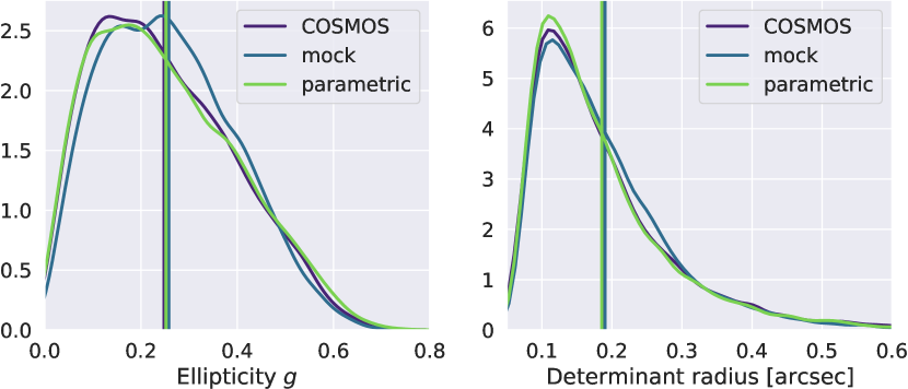
(a) Marginal distributions

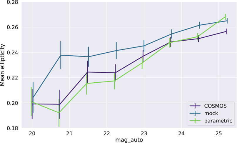
(b) Ellipticity as a function of magnitude

Figure 6: Comparison of second-order moments between COSMOS galaxies, parametric fits, and VAE samples. The vertical lines in (a) indicate the means of the respective distributions. The error bars in (b) indicate the 1-$\sigma$ error on the mean ellipticity.

Figure 6 compares the marginal distribution of determinant radius $\sigma$ and ellipticity $|g|$ for the three different samples. We find excellent agreement between the reference COSMOS distribution and galaxies generated from the generative model, with a 4% difference in mean ellipticity and 1% difference in mean size.

In addition to comparing the overall distribution of size and ellipticity, we can test the quality of the conditional sampling with Figure 7 showing for each pair of real and mock galaxy the difference in size and flux, as a function of the corresponding conditional variable. The red line in these plots shows the median of the corresponding residual distribution in bins of size and magnitude. On these simple statistics, we find that the conditioning is largely unbiased, but note an overall $\sim 27\%$ scatter in size, and $\sim 0.3$ in magnitude. For these two properties however, while the conditioning is not extremely precise, a desired size and flux can always be imposed after sampling from the generative model, using GalSim light profile manipulation utilities.

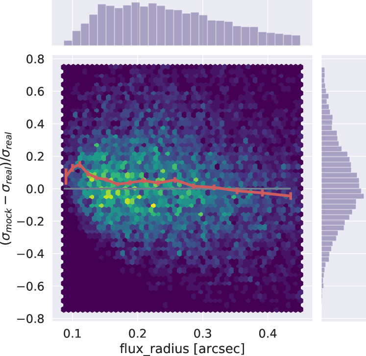
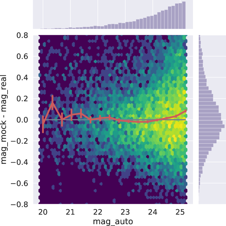
Figure 7: Comparison of measured determinant radius and magnitude between pairs of COSMOS galaxies and VAE samples, as a function of half light radius and magnitude of the real galaxy, which are also used to condition the corresponding VAE samples. The solid red line represents the median of the difference in size and flux, in bins of the corresponding conditional quantities. The error bars indicate the $1-\sigma$ uncertainty on that median value.

4.4.2 Morphological statistics

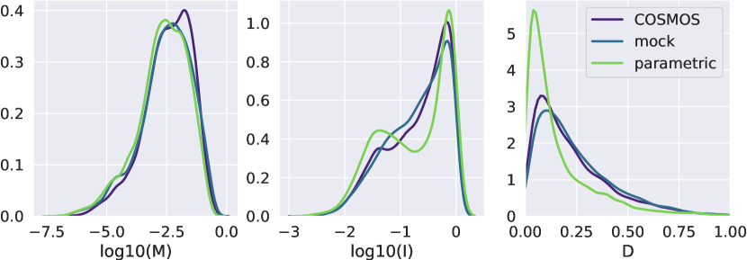
Figure 8: Comparison of marginal MID statistics evaluated on parametric galaxies (left), real COSMOS galaxies (center), samples from the generative model (right).

To further quantitatively compare our generated galaxy sample to the reference training set, we turn to higher order morphological statistics. In this work we primarily make use of the multi-mode (M), intensity (I), and Deviation (D) statistics introduced in Freeman et al. (2013), which are specifically designed to identify disturbed morphologies. We direct the interested reader to Freeman et al. (2013) for a thorough description of these statistics and a comparison to standard CAS statistics (Conselice, 2003), and we briefly introduce them below:

• M(ulti-mode) statistic: detects multimodality in a galaxy light profile as a ratio of area between the largest and second largest contiguous group of pixels above a threshold itself optimized as to maximize this statistic. M tends to 1 if the light profile exhibits a double nucleus, and to 0 if the image is unimodal.

• I(ntensity) statistic: Similar to the M statistic but computes a ratio of integrated flux between the two most intense contiguous groups of pixels in the image. I tends to 1 for two equally intense nuclei, and to 0 if the flux of the brightest nucleus dominates.

• D(eviation) statistic: Measures the distance between the local intensity maximum identified as part of the I statistic to the centroid of the light profile computed by a simple first-order moment computation. This distance is scaled by the size of the segmentation map of the object and is therefore below 1, tending towards 0 for symmetrical galaxies.

In addition to these statistics, we also evaluate the Gini coefficient and M20 statistic (Lotz et al., 2004). These respectively measure the relative distribution of pixel fluxes, and the second-order moment of the brightest 20% pixels.

Figure 8 illustrates the distribution of MID statistics for samples of parametric, mock, and real images. While we do not see a strong deviation in term of the M statistic, the distributions of I and D statistics are significantly different for parametric galaxies, while mock and real galaxies appear to be very similar. More specifically, for the I statistic, we note that parametric fits exhibit an under-density around I $\simeq 0.1$ compared to real COSMOS galaxies. We observed that in this range of I values, multimodal real galaxies are found whereas these do not exist in the monotonic parametric models. As a result, this region is depleted for parametric models. We find that the fits to multimodal COSMOS galaxies from this region are preferentially scattered towards I $=1$ for large structured galaxies, as the modes identified on noisy monotonic profile tend to be from the same neighbourhood and have very similar fluxes. On the other hand, for bright and concentrated galaxies, the parametric fits are scattered to lower I values; in this case the central peak is also clearly identified in the parametric fit, and a second peak, only due to noise, is necessarily artificial and at far lower fluxes. This explains why we observe this bi-modal shape of the $\log($I$)$ distribution of parametric galaxies. For the D statistic, we similarly see a significantly higher concentration near D $=0$ for parametric profiles compared to real COSMOS galaxies. This is consistent with the definition of this statistic as parametric profiles are symmetric, hence low D statistic. These results for parametric profiles are therefore completely consistent with one’s expectations for Sérsic or Bulge+Disk models with an additional noise field.

By comparison, our mock galaxy images are more consistent with real galaxies, and the fact that they do not exhibit the same failure modes as parametric profiles indicates that the light profiles generated by the deep generative models are indeed less symmetrical and more multimodal than simple profiles. This difference can also be seen in the 2d I-D histograms of 9(b).

9(a) provides a similar comparison, but in the Gini-M20 plane, typically used to identify galaxy mergers or galaxies with disturbed morphologies (Lotz et al., 2004). In this plane, galaxies with simpler, less perturbed morphologies are typically found on the right side of the distribution, towards lower M20. On 9(a), we notice a clear depletion of parametric galaxies at higher M20 and low Gini index (lower left corner) compared to real galaxies. These galaxies seem to have migrated to the right side of the plot, which corresponds to smoother morphologies. We are therefore clearly seeing through this plot that parametric profiles are smoother, less disturbed, than real COSMOS galaxies. On the contrary, no such trend can be identified when comparing COSMOS galaxies to mock galaxies from the Flow-VAE, confirming that under the common Gini-M20 statistic, galaxies sampled from the generative model are also significantly more realistic than simple parametric profiles.

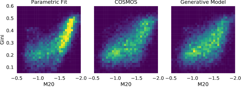
(a) Gini-M20 statistics

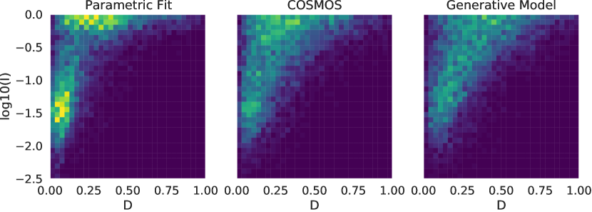
(b) I-D statistics

Figure 9: Comparison of morphology statistics Gini-M20 (a) and I-D (b) evaluated on parametric galaxies (left), real COSMOS galaxies (center), samples from the generative model (right). The colormap is linear. On the Gini-M20 plane, more disturbed morphologies are typically found on the left side of the plot, while smoother morphologies are found to the right.

5 Discussion

We have presented a framework for building and fitting generative models of galaxy morphology, combining deep learning and physical modeling elements allowing us to explicitly account for the PSF and noise. With this hybrid approach, the intrinsic morphology of galaxies can effectively be decoupled from the observational PSF and noise, which is essential for the use of these generative models in practice. We have further demonstrated a new type of conditional generative model, allowing us to condition galaxy morphology on physical galaxy properties. On a sample of galaxies from the HST/ACS COSMOS survey with a limiting magnitude of 25.2 in F814W, we have demonstrated that this deep learning approach to modeling galaxy light profiles not only reproduces distributions of second order moments of the light profiles (i.e. size and ellipticity), but more importantly, is more accurate than conventional parametric light profiles (Sérsic or Bulge+Disk) when considering a set of morphological summary statistics particularly sensitive to non-monotonicity. We further note that while any deficiencies in modeling second order moments can be trivially addressed by dilation or shearing, these higher order statistics could otherwise not be easily imposed.

In this section, we now discuss future prospects for applications of these tools as well as further potential improvements and developments.

A first important point highlighted by this work is that when encapsulated within a physical forward model of the instrument, these latent variable generative models can be trained to learn denoised and PSF-deconvolved light profiles. This means that in future work, it will be possible to combine data from ground- and space-based instruments to jointly constrain the same deep and high resolution morphology models. This is to be compared to the current requirement of having access to dedicated deep space based observations which remains limited in quantity and raises concerns such as cosmic variance (Kannawadi et al., 2015). Using HSC deep fields for instance, fitting the morphology model to individual exposures would allow us to profit from the overall depth of the survey as well as from the good seeing exposures bringing more constraints on small scales.

Although we have not emphasized this aspect of our approach in the previous section, the light profiles learned by our models being unconvolved from the PSF, they may contain details beyond the original band-limit of the survey. Thanks to the small amount of Total Variation regularization added to the training loss in Section 4.2, we find in practice that the model does not introduce obviously unphysical high frequencies or artifacts. Therefore, it may be possible to use these galaxy models with a PSF slightly smaller than a typical COSMOS PSF used for training, which can be thought of as some sort of extrapolation to higher band-limits. We caution the user against such a use however, as any details smaller than the original COSMOS resolution are not constrained from data and are purely the results of implicit priors and inductive biases. Testing the impacts of this explicitly, for example by learning a generative model from a version of the COSMOS images degraded in resolution and comparing to the original-resolution images, could be one way to understand the degree to which any extrapolation is possible. This test is left for future work.

As an alternative to learning fully deconvolved light profiles, we also explored partial deconvolution, where galaxies are modeled at a standardized effective PSF only slightly smaller than the training PSFs. In our experiments, although it made the training slightly more stable, it did not significantly affect the performance of the trained model. We did not pursue this option further, but future work using different architectures, especially GANs, may find partial deconvolution advantageous.

Another highlight of this work is the ability to condition galaxy morphology on other physical properties of the object. In an image simulation context, this makes it possible to tie morphology to physical parameters available in mock galaxy catalogs (e.g., stellar mass, colour, magnitude, redshift). This will be crucial for producing complex and realistic survey images accounting jointly for galaxy clustering, photometry, and morphology.

Beyond image simulations, generative models can be regarded as a general solution for building fully data-driven signal priors which can be used in a range of astronomical imaging inverse problems such as denoising, deconvolution, or deblending. This idea has been for instance explored in the context of deblending in Arcelin et al. (2020) using a VAE to learn a model of isolated galaxies light profiles, or in Lanusse et al. (2019) using an autoregressive pixelCNN++ (Oord et al., 2016) model trained on isolated galaxy images as a prior for deblending by solving a maximum a posteriori optimization problem. The usefulness of latent variable models for solving general inverse problems was further explored in Böhm et al. (2019), which illustrates how a Flow-VAE such as the one introduced in this work can be used to recover full posteriors on problems such as deconvolution, denoising, and inpainting.

One open question that has been only partially addressed so far is how to validate the quality of the morphology models. As illustrated in this work, parametric light profiles match by design real galaxies in terms of zeroth, first, and second moments (Figure 6), while metrics based on higher order statistics (e.g., Figure 9, Figure 8) are able to detect significant departures in morphology. While our particular choice of higher order statistics has proven powerful enough to demonstrate a qualitative gain in morphology over simple parametric profiles, we have however no guarantee that this set of statistics is sufficient to fully characterize galaxy morphology. Instead of relying on the carefully crafted metrics which are conventionally used to study galaxy morphologies, recent work has focused on using generative models for anomaly detection. In the first application of these methodologies to astrophysics (Zanisi et al., 2020) have for instance demonstrated that a method based on the Log Likelihood Ratio approach of Ren et al. (2019) is capable of identifying morphology discrepancies between IllustrisTNG (Nelson et al., 2019) and SDSS (Abazajian et al., 2009; Meert et al., 2015) galaxies.

More fundamentally, even if we had access to a set of sufficient statistics to detect deviations between real and generated galaxies, it would remain unclear how close the model would need to match the real morphologies in terms of these statistics in order to satisfy the requirements of a particular scientific application. As an example, let us consider the specific case of calibrating weak lensing shear measurements with image simulations. It is known that the distribution of galaxies ellipticities needs to be modeled with great accuracy (Viola et al., 2014), and precise requirements can be set in terms of ellipticities. These are however necessary but not sufficient conditions; shear couples second-order moments (from which the ellipticity is derived) to higher-order moments of the light profiles (Massey et al., 2007; Bernstein, 2010; Zhang & Komatsu, 2011), which makes calibration sensitive to morphological details and substructure. Although we have various higher-order statistics at our disposal, defining a set of requirements to ensure accurate calibration is a difficult task and such requirements have never been rigorously quantified in practice.

Finally, here we have proposed a very specific generative model architecture. In our experiments we found this approach of a hybrid VAE and normalizing flow model to be robust and flexible while providing good quality samples. However, we do not expect this model to remain a state-of-the-art solution, and on the contrary we welcome and encourage additional efforts from the community to develop better models. In that spirit, we have put significant efforts into building galaxy2galaxy (g2g for short), a framework for training, evaluating, and exporting generative models on standard datasets such as the COSMOS sample used in this work. In addition, we have developed the galsim_hub extension to the GalSim software, which allows us to integrate models trained with g2g directly as GalSim GSObjects which can then be manipulated in the GalSim framework like any other analytic light profile. More details on galsim_hub can be found in Appendix A.

In the spirit of reproducible and reusable research, the code developed for this paper has been packaged in the form of two Python libraries

• Galaxy2Galaxy: Framework for training and exporting generative models

  https://github.com/ml4astro/galaxy2galaxy

• GalSim-Hub: Framework for integrating deep generative models as part of GalSim image simulation software.

  https://github.com/mcwilliamscenter/galsim_hub

The scripts used to train the models presented in this work as well as producing all the figures can be found at this link:

https://github.com/mcwilliamscenter/deep_galaxy_models

Data Availability

The HST/ACS COSMOS data used in this article are available at http://doi.org/10.5281/zenodo.3242143. The images and statistics obtained with the generative model are available at http://doi.org/10.5281/zenodo.3975700.

Appendix A GalSim-Hub: online repository for trained models

As a way to easily interface deep generative models with existing simulation pipelines based on the GalSim software, we introduce GalSim-Hub: an online repository of pre-trained models which can directly used within GalSim as any other light profiles.

Concretely, GalSim-Hub is based on the TensorFlow Hub library which allows for TensorFlow models to be saved, loaded, and executed similarly to a conventional Python function within a Python library. In addition to a plain TensorFlow Hub module, GalSim-Hub also specifies some key metadata such as the pixel resolution of the generated image, or input fields required by the module for conditional sampling. At sampling time, the library will generate an un-convolved image by drawing from the generative model, and turn that image into a GalSim InterpolatedImage object which can then be used as any other type of light profile.

To make it easy for researchers to exchange trained deep generative models of galaxy morphology, GalSim-Hub also provides an online repository for community-maintained models directly from the project GitHub repository: https://github.com/mcwilliamscenter/galsim_hub .

Figure 10 illustrates a minimal working example of generating a list of galaxies conditioned on size and magnitude from a pre-trained model available from the online repository.

import galsimimport galsim_hubfrom astropy.table import Table# Load generative model from the online repositorymodel = galsim_hub.GenerativeGalaxyModel(’hub:Lanusse2020’)# Defines the input conditionscat = Table([[5., 10. ,20.],             [24., 24., 24.],             [0.5, 0.5, 0.5]],             names=[’flux_radius’, ’mag_auto’, ’zphot’])# Sample light profiles for these parametersims = model.sample(cat)# Define a PSFpsf = galsim.Gaussian(sigma=0.06)# Convolve by PSFims = [galsim.Convolve(im, psf) for im in ims]

Figure 10: Example of sampling galaxies from the generative model conditioned on size and magnitude with GalSim Hub. The library will automatically download from the online repository models referenced with “hub:xxxx” so that no manual user intervention is necessary to run a script.

References

- Abadi et al. (2016) Abadi M., et al., 2016, in 12th USENIX Symposium on Operating Systems Design and Implementation (OSDI 16). pp 265–283, https://www.usenix.org/system/files/conference/osdi16/osdi16-abadi.pdf
- Abazajian et al. (2009) Abazajian K. N., et al., 2009, Astrophysical Journal, Supplement Series, 182, 543
- Arcelin et al. (2020) Arcelin B., Doux C., Aubourg E., Roucelle C., 2020, 14, 1
- Bernstein (2010) Bernstein G. M., 2010, Monthly Notices of the Royal Astronomical Society, 406, 2793
- Bernstein & Jarvis (2002) Bernstein G. M., Jarvis M., 2002, The Astronomical Journal, 123, 583
- Böhm et al. (2019) Böhm V., Lanusse F., Seljak U., 2019, pp 1–9
- Bosch et al. (2017) Bosch J., et al., 2017, ] 10.1093/pasj/xxx000, 00, 1
- Che et al. (2016) Che T., Li Y., Jacob A. P., Bengio Y., Li W., 2016, 5th International Conference on Learning Representations, ICLR 2017 - Conference Track Proceedings, pp 1–13
- Conselice (2003) Conselice C. J., 2003, ApJS, 147, 1
- Cremer et al. (2018) Cremer C., Li X., Duvenaud D., 2018, 35th International Conference on Machine Learning, ICML 2018, 3, 1749
- Dillon et al. (2017) Dillon J. V., et al., 2017
- Dinh et al. (2016) Dinh L., Sohl-Dickstein J., Bengio S., 2016, 5th International Conference on Learning Representations, ICLR 2017 - Conference Track Proceedings
- Engel et al. (2017) Engel J., Hoffman M., Roberts A., 2017, pp 1–19
- Fenech Conti et al. (2017) Fenech Conti I., Herbonnet R., Hoekstra H., Merten J., Miller L., Viola M., 2017, Monthly Notices of the Royal Astronomical Society, 467, 1627
- Foreman-Mackey et al. (2020) Foreman-Mackey D., et al., 2020, daft-dev/daft: Minor bugfix, doi:10.5281/zenodo.3747801, https://doi.org/10.5281/zenodo.3747801
- Freeman et al. (2013) Freeman P. E., Izbicki R., Lee A. B., Newman J. A., Conselice C. J., Koekemoer A. M., Lotz J. M., Mozena M., 2013, Monthly Notices of the Royal Astronomical Society, 434, 282
- Fussell & Moews (2019) Fussell L., Moews B., 2019, Monthly Notices of the Royal Astronomical Society, 485, 3215
- Germain et al. (2015) Germain M., Gregor K., Murray I., Larochelle H., Ed I. M., Uk A. C., 2015, Proceedings of The 32nd International Conference on Machine Learning, 37, 881
- Goodfellow et al. (2014) Goodfellow I., Pouget-Abadie J., Mirza M., 2014, arXiv preprint arXiv: …, pp 1–9
- Griffith et al. (2012) Griffith R. L., et al., 2012, The Astrophysical Journal Supplement Series, 200, 9
- He et al. (2019) He J., Spokoyny D., Neubig G., Berg-Kirkpatrick T., 2019, pp 1–15
- Hirata & Seljak (2003) Hirata C., Seljak U., 2003, Monthly Notices of the Royal Astronomical Society, 343, 459
- Hunter (2007) Hunter J. D., 2007, Computing In Science & Engineering, 9, 90
- Kacprzak et al. (2019) Kacprzak T., et al., 2019, pp 1–31
- Kannawadi et al. (2015) Kannawadi A., Mandelbaum R., Lackner C., 2015, Monthly Notices of the Royal Astronomical Society, 449, 3597
- Kannawadi et al. (2019) Kannawadi A., et al., 2019, Astronomy and Astrophysics, 624
- Kingma & Ba (2015) Kingma D. P., Ba J. L., 2015, International Conference on Learning Representations 2015, pp 1–15
- Kingma & Welling (2013) Kingma D. P., Welling M., 2013, 587
- Kingma et al. (2016) Kingma D. P., Salimans T., Jozefowicz R., Chen X., Sutskever I., Welling M., 2016, Nips, pp 1–8
- Kluyver et al. (2016) Kluyver T., et al., 2016, in ELPUB.
- Koekemoer et al. (2007) Koekemoer A., et al., 2007, Astrophysical Journal, Supplement Series, 172, 196
- Korytov et al. (2019) Korytov D., et al., 2019
- LSST Dark Energy Science Collaboration (2012) LSST Dark Energy Science Collaboration 2012, pp 1–133
- Lanusse et al. (2019) Lanusse F., Melchior P., Moolekamp F., 2019
- Laureijs et al. (2011) Laureijs R., et al., 2011, preprint, p. arXiv:1110.3193
- Leauthaud et al. (2007) Leauthaud A., et al., 2007, The Astrophysical Journal Supplement Series, 172, 219
- Leistedt et al. (2019) Leistedt B., Hogg D. W., Wechsler R. H., DeRose J., 2019, The Astrophysical Journal, 881, 80
- Lotz et al. (2004) Lotz J. M., Primack J., Madau P., 2004, The Astronomical Journal, 128, 163
- Mandelbaum et al. (2012) Mandelbaum R., Lackner C., Leauthaud A., Rowe B., 2012, COSMOS real galaxy dataset, doi:10.5281/zenodo.3242143
- Mandelbaum et al. (2014) Mandelbaum R., et al., 2014, The Astrophysical Journal Supplement Series, 212, 5
- Mandelbaum et al. (2015) Mandelbaum R., et al., 2015, Monthly Notices of the Royal Astronomical Society, 450, 2963
- Mandelbaum et al. (2018) Mandelbaum R., et al., 2018, Monthly Notices of the Royal Astronomical Society, 481, 3170
- Massey et al. (2004) Massey R., Refregier A., Conselice C. J., Bacon D. J., 2004, Monthly Notices of the Royal Astronomical Society, 348, 214
- Massey et al. (2007) Massey R., Rowe B., Refregier A., Bacon D. J., Bergé J., 2007, Monthly Notices of the Royal Astronomical Society, 380, 229
- Maturi (2017) Maturi M., 2017, Monthly Notices of the Royal Astronomical Society, 471, 750
- Meert et al. (2015) Meert A., Vikram V., Bernardi M., 2015, Monthly Notices of the Royal Astronomical Society, 446, 3943
- Melchior et al. (2018) Melchior P., Moolekamp F., Jerdee M., Armstrong R., Sun A.-L., Bosch J., Lupton R., 2018, Astronomy and Computing, 24, 129
- Nelson et al. (2019) Nelson D., et al., 2019, Computational Astrophysics and Cosmology, 6, 2
- Oord et al. (2016) Oord A. v. d., Kalchbrenner N., Kavukcuoglu K., 2016, International Conference on Machine Learning (ICML), 48
- Papamakarios et al. (2017) Papamakarios G., Pavlakou T., Murray I., 2017, ] 10.1080/0955300001003760
- Perez & Granger (2007) Perez F., Granger B. E., 2007, Computing in Science & Engineering, 9, 21
- Plazas et al. (2019) Plazas A. A., Meneghetti M., Maturi M., Rhodes J., 2019, Monthly Notices of the Royal Astronomical Society, 482, 2823
- Price-Whelan et al. (2018) Price-Whelan A. M., et al., 2018, The Astronomical Journal, 156, 123
- Ravanbakhsh et al. (2017) Ravanbakhsh S., Lanusse F., Mandelbaum R., Schneider J., Póczos B., 2017, 31st AAAI Conference on Artificial Intelligence, AAAI 2017, pp 1488–1494
- Regier et al. (2015) Regier J., McAuliffe J., Prabhat 2015, Neural Informational Processing Systems (NIPS) Workshop: Advances in Approximate Bayesian Inference, 2, 1
- Reiman & Göhre (2019) Reiman D. M., Göhre B. E., 2019, Monthly Notices of the Royal Astronomical Society, 485, 2617
- Ren et al. (2019) Ren J., Liu P. J., Fertig E., Snoek J., Poplin R., DePristo M. A., Dillon J. V., Lakshminarayanan B., 2019
- Rezende & Mohamed (2015) Rezende D. J., Mohamed S., 2015, Proceedings of the 32nd International Conference on Machine Learning, 37, 1530
- Robitaille et al. (2013) Robitaille T. P., et al., 2013, Astronomy & Astrophysics, 558, A33
- Ronneberger et al. (2015) Ronneberger O., Fischer P., Brox T., 2015, CoRR
- Rowe et al. (2015) Rowe B. T. P., et al., 2015, Astronomy and Computing, 10, 121
- Salimans et al. (2016) Salimans T., Goodfellow I., Zaremba W., Cheung V., Radford A., Chen X., 2016, Advances in Neural Information Processing Systems, pp 2234–2242
- Salimans et al. (2017) Salimans T., Karpathy A., Chen X., Kingma D. P., 2017, pp 1–10
- Samuroff et al. (2017) Samuroff S., et al., 2017, 000
- Sánchez et al. (2020) Sánchez F. J., et al., 2020, 000
- Schawinski et al. (2017) Schawinski K., Zhang C., Zhang H., Fowler L., Santhanam G. K., 2017, Monthly Notices of the Royal Astronomical Society: Letters, 467, L110
- Scoville et al. (2007a) Scoville N., et al., 2007a, The Astrophysical Journal Supplement Series, 172, 1
- Scoville et al. (2007b) Scoville N., et al., 2007b, The Astrophysical Journal Supplement Series, 172, 38
- Shazeer & Stern (2018) Shazeer N., Stern M., 2018, 35th International Conference on Machine Learning, ICML 2018, 10, 7322
- Sheldon & Huff (2017) Sheldon E. S., Huff E. M., 2017, ] 10.3847/1538-4357/aa704b
- Smith & Geach (2019) Smith M. J., Geach J. E., 2019, 0
- Somerville & Davé (2015) Somerville R. S., Davé R., 2015, Annual Review of Astronomy and Astrophysics, 53, 51
- Sønderby et al. (2016) Sønderby C. K., Raiko T., Maaløe L., Sønderby S. K., Winther O., 2016, Nips
- Spergel et al. (2015) Spergel D., et al., 2015, preprint
- Troxel et al. (2019) Troxel M. A., et al., 2019, 23, 1
- Vaswani et al. (2018) Vaswani A., et al., 2018, AMTA 2018 - 13th Conference of the Association for Machine Translation in the Americas, Proceedings, 1, 193
- Viola et al. (2014) Viola M., Kitching T. D., Joachimi B., 2014, Monthly Notices of the Royal Astronomical Society, 439, 1909
- Waskom et al. (2020) Waskom M., et al., 2020, mwaskom/seaborn: v0.10.1 (April 2020), doi:10.5281/zenodo.3767070, https://doi.org/10.5281/zenodo.3767070
- Willett et al. (2013) Willett K. W., et al., 2013, Monthly Notices of the Royal Astronomical Society, 435, 2835
- Zanisi et al. (2020) Zanisi L., et al., 2020, 24, 1
- Zhang & Komatsu (2011) Zhang J., Komatsu E., 2011, Monthly Notices of the Royal Astronomical Society, 414, 1047
- Zhang et al. (2015) Zhang J., Luo W., Foucaud S., 2015, Journal of Cosmology and Astroparticle Physics, 2015
- Zhang et al. (2016) Zhang H., Xu T., Li H., Zhang S., Huang X., Wang X., Metaxas D. N., 2016, CoRR, abs/1612.0