Risk-Sensitive Markov Decision Processes with Combined Metrics of Mean and Variance

Abstract

This paper investigates the optimization problem of an infinite stage discrete time Markov decision process (MDP) with a long-run average metric considering both mean and variance of rewards together. Such performance metric is important since the mean indicates average returns and the variance indicates risk or fairness. However, the variance metric couples the rewards at all stages, the traditional dynamic programming is inapplicable as the principle of time consistency fails. We study this problem from a new perspective called the sensitivity-based optimization theory. A performance difference formula is derived and it can quantify the difference of the mean-variance combined metrics of MDPs under any two different policies. The difference formula can be utilized to generate new policies with strictly improved mean-variance performance. A necessary condition of the optimal policy and the optimality of deterministic policies are derived. We further develop an iterative algorithm with a form of policy iteration, which is proved to converge to local optima both in the mixed and randomized policy space. Specially, when the mean reward is constant in policies, the algorithm is guaranteed to converge to the global optimum. Finally, we apply our approach to study the fluctuation reduction of wind power in an energy storage system, which demonstrates the potential applicability of our optimization method.

Keywords: Markov decision process, risk-sensitive, mean and variance, sensitivity-based optimization

1 Introduction

The theory of Markov decision processes (MDPs) is widely used to analyze and optimize the performance of a stochastic dynamic system. In the framework of MDPs, $R_{T}$ is denoted as the accumulated (discounted or undiscounted) rewards until time $T$, which is a random variable. Many studies of MDPs focus on the discounted or long-run average performance criteria, i.e., maximization of $\mathbb{E}[R_{T}]$. However, its variance $\sigma^{2}[R_{T}]$ is also an important metric in practical problems, which can reflect the factors of risk, fairness, quality or safety. For example, the mean-variance analysis for the risk management in financial portfolio or hedging (Kouvelis et al., 2018), the fairness of customers served in queueing systems (Avi-Itzhak and Levy, 2004), the power quality and safety of renewable energy to electricity grid (Li et al., 2014), the optimal advertising of fashion markets and supply chain management (Chiu et al., 2018; Zhang et al., 2020), etc. Optimization theory of risk-sensitive MDPs considering not only the average metric but also the variance metric is an important problem attracting continued attention in the literature.

However, the optimization of the variance metric does not fit a standard model of MDPs because of the non-additive variance function. The value of the variance function will be affected by actions of not only the current stage but also the future stages (Bertsekas, 2005; Feinberg and Schwartz, 2002; Puterman, 1994). Thus, the Bellman optimality equation does not hold and the principle of time consistency (roughly speaking, if a decision at time $t+1$ is optimal, then it should constitute part of optimal decisions at time $t$) in dynamic programming fails (Ruszczyński, 2010; Shapiro, 2009). One main thread of studying the variance optimization problem lays in the framework of the MDP theory, which aims at minimizing the variance after the mean performance already achieves optimum. For the policy subset where the mean already achieves optimum, the variance minimization problem is equivalent to another standard MDP with a new average cost criterion. Interested readers can refer to related papers in the literature, such as the work by Cao and Zhang (2008) about the $n$-bias optimality of MDPs, the works by Guo and Song (2009); Guo et al. (2012) about discounted MDPs, and the work by Hernandez-Lerma et al. (1999) about average MDPs, just name a few. For these equivalent MDPs, traditional approaches like dynamic programming or policy iteration can be used to minimize the variance of MDPs.

Another thread of studying the variance-related optimization problem is the policy gradient approach for risk-sensitive MDPs (Prashanth and Ghavamzadeh, 2013; Tamar et al., 2013), which is more from the algorithmic viewpoint in reinforcement learning. In this scenario, the policy is usually parameterized by sophisticated functions, e.g., neural networks. In general, such optimization problem is not a standard MDP (a parameterized one) and the policy iteration is not applicable. For such scenarios, stochastic gradient-based algorithms are usually adopted to approach to a local optimal solution. Although neural networks have strong policy representation capability, such gradient-based algorithms usually converge slowly and suffer from some intrinsic deficiencies, such as trap of local optimum, difficulty of selecting step sizes, and sensitivity to initial points. Seeking policy iteration type algorithms is a promising attempt to study the MDPs with variance criteria. A recent study investigates the variance minimization problem regardless of the optimality of mean performance from the perspective of the sensitivity-based optimization, where algorithms with a policy iteration type are developed for the variance minimization problem of MDPs with averages and parameterized policies, respectively (Xia, 2016, 2018b). It is worth noting that there exist other risk-sensitive metrics besides the variance-related one. For example, exponential utility function is also a risk-sensitive metric since the first two orders of Taylor expansions of exponential utility include the mean and the variance (Bäuerle and Jaśkiewicz, 2015; Borkar, 2002; Guo and Zhang, 2019). Percentile-related criterion, VaR (Value at Risk), and CVaR (Conditional VaR) are other widely studied risk-sensitive metrics in the field of finance and economy (Chow et al., 2015; Delage and Mannor, 2010; Fu et al., 2009; Gao et al., 2017; Hong et al., 2014). Motivated by the modern theory of coherent risk measures (Artzner et al., 1999), time-consistent Markov risk measures are also studied from another point of view in risk-aware MDPs literature (Ruszczyński, 2010; Ruszczyński and Shapiro, 2006). Haskell and Jain (2013) study the stochastic dominance of accumulated rewards rather than the expectation of rewards, which is another interesting way to study the risk-aware metrics in MDPs.

In the literature, some studies consider the performance optimization of mean and variance together, which is called the mean-variance optimization. The pioneering work of mean-variance optimization is initiated by Markowitz (1952), the Nobel Laureate in Economics. Intensive attention has been paid during past decades and the mathematical model is extended from single-stage static problem to multi-stage dynamic one. Markov models are usually adopted when we study the mean-variance optimization in a stochastic dynamic scenario. The related works on the dynamic mean-variance optimization can be categorized into three classes. The first one is to maximize the mean performance at the condition that the variance is less than a given amount. The second one is to minimize the variance while keeping the mean performance larger than a given amount. The third one is to optimize the combination of the mean and the variance together, such as maximizing the Sharpe ratio $\frac{\mathbb{E}[R_{T}]}{\sigma[R_{T}]}$ or the weighted combination $\mathbb{E}[R_{T}]-\beta\sigma^{2}[R_{T}]$. Chung (1994) and Sobel (1994) study the mean-variance optimization in a regime of long-run average MDPs, by converting the constrained MDP problem to a mathematical programming problem. Numerical algorithms are also studied for the multistage mean-variance optimization problem from the viewpoint of mathematical programming (Parpas and Rustem, 2007). For discounted MDPs, the variance minimization problem with a given discounted average performance can be converted to an equivalent discounted MDP with a new cost function (Huang, 2018; Huo et al., 2017; Xia, 2018a), and traditional MDP methods such as policy iteration are applicable. In some general settings, it has been shown that the mean-variance optimization problem in MDPs is NP-hard (Mannor and Tsitsiklis, 2013). Another way to study the mean-variance optimization is from the perspective of optimal control, in which the model is usually continuous time or even continuous state and the optimality structures of control laws are investigated for specific scenarios (Zhou and Li, 2000; Zhou and Yin, 2004). In recent years, reinforcement learning attracts intensive attention for the great success of AlphaGo. Although most reinforcement learning algorithms focus on discounted criterion, some policy gradient algorithms are also investigated to optimize the combined metrics of mean and variance (Borkar, 2010; Tamar et al., 2012). However, such gradient-based approach still suffers from the deficiency of local optimum and slow convergence. On the other hand, as we know, there are three categories of approaches to solve MDP problems: policy iteration, value iteration, and policy gradient, where the policy iteration is a classical and important approach. Although the algorithmic complexity of the policy iteration is still an open problem (Littman et al., 1995), it is observed that the policy iteration usually converges very fast in most cases. Therefore, it is promising to develop policy iteration type algorithms to solve the mean-variance optimization problem.

In this paper, we study the optimization of the mean-variance combined metric in the framework of MDPs. The objective is to find the optimal policy that maximizes the mean minus variance metrics, $\mathbb{E}[R_{T}]-\beta\sigma^{2}[R_{T}]$. Different coefficients $\beta$ tradeoff the weights between the mean and the variance. Since the variance-related metric is not additive, this dynamic optimization problem does not fit the standard model of MDPs. The time consistency of dynamic programming is not valid and the Bellman optimality equation does not hold. We study this problem from a new perspective called the theory of sensitivity-based optimization (Cao, 2007), which is rooted from the theory of perturbation analysis (Ho and Cao, 1991) and largely extended to stochastic dynamic systems with Markov models. The key idea of the sensitivity-based optimization is to utilize the performance difference and derivative information to search the optimal policy. This theory is applicable for general Markov systems and it does not require an additive cost function. For the mean-variance combined metric, we derive a difference formula which quantifies the difference of the combined metrics under any two policies. The coupling effect caused by the non-additive variance function can be decoupled by a square term in the difference formula. Based on the difference formula, we derive a method to strictly improve the system mean-variance metrics. A necessary condition of the optimal policy is also derived. We further prove that the optimal policy with the maximal mean-variance combined metric can always be achieved in the deterministic policy space. A policy iteration type algorithm is developed to find the optimal policy, which is proved to converge to a local optimum both in the mixed and randomized policy space. Moreover, this algorithm can find the global optimum if the mean reward remains constant for different policies. Some exploration techniques are also discussed to improve the global search capability of the algorithm. Finally, we use an example in a renewable energy storage system to demonstrate that our approach can effectively reduce the fluctuation of the total output power, which improves the output power quality and reduces the stability risk of power grid. The local convergence and the global convergence of our approach are both demonstrated in different scenarios of this example.

The main contributions of the paper are as follows. We use the sensitivity-based optimization theory to study the performance optimization of mean-variance combined metrics in Markov systems, which is a new perspective different from the traditional dynamic programming. Although the principle of dynamic programming is not applicable, we derive a difference formula to quantify the changing behaviors of mean-variance combined metrics with respect to different policies. Optimality conditions and a policy iteration type algorithm for optimal policies are also derived. To the best of our knowledge, our paper is the first work that a policy iteration type algorithm is developed to optimize the mean-variance combined metrics in MDPs. Compared with traditional gradient-based algorithms, policy iteration usually has a much faster convergence speed, which is partly demonstrated by our numerical experiments.

This paper is substantially extended based on its conference version (Xia and Yang, 2019), where the main theorems, algorithms, and experiments are not presented. The difference of this paper from our previous work (Xia, 2016) is that this paper optimizes both the mean and variance metrics together, while Xia (2016) only minimizes the variance metric without any consideration of the mean performance. It is important to consider the mean and variance metrics together in real life. Many works about dynamic mean-variance optimization focus on the variance of accumulated discounted rewards at a terminal stage, where the contraction operator is a key tool. There are much less works studying the mean-variance optimization of rewards in the sense of long-run averages, where the contraction operator is not applicable. Therefore, our work on the long-run mean-variance combined metrics could give a complementary result to the whole theory of mean-variance optimization. We hope that this paper could shed light on studying the dynamic mean-variance optimization, especially in the scenario with long-run average metrics (instead of discounted ones) and policy iteration type algorithms (instead of gradient ones).

The remainder of the paper is organized as follows. In Section 2, we formulate the performance optimization problem of mean-variance combined metrics under the framework of MDPs. The main challenge of this problem is also discussed. In Section 3, we use the sensitivity-based optimization theory to derive the difference formula for the mean-variance combined metrics. Optimality structures and necessary condition of the optimal policy are also derived. Furthermore, we develop an iterative algorithm to find the optimal policy in Section 4. The convergence analysis of the algorithm is also studied. In Section 5, we use an example of renewable energy storage systems to numerically illustrate the local and global convergence of our approach, respectively. Finally, we conclude this paper and discuss some future research topics in Section 6.

2 Problem Formulation

We consider a discrete time Markov decision process. The state space and the action space are both finite and denoted as $\mathcal{S}:=\{1,2,\cdots,S\}$ and $\mathcal{A}:=\{a_{1},a_{2},\cdots,a_{A}\}$, respectively. In general, $\mathcal{A}$ can also be state-dependent, i.e., $\mathcal{A}(i)$ and $i\in\mathcal{S}$, but we omit this case for simplicity of representation. A stationary policy is a mapping from the state space to the action space, $d:\mathcal{S}\rightarrow\mathcal{A}$, where $d$ is deterministic since its optimality is proved in the later section. The stationary policy space is denoted as $\mathcal{D}$. At each state $i\in\mathcal{S}$, an action $a=d(i)$ will be adopted if policy $d\in\mathcal{D}$ is being employed. Then the system will transit to the next state $j$ with transition probability $p^{a}(i,j)$ and an instant reward $r(i,a)$ will be incurred, $i,j\in\mathcal{S}$. We denote $\bm{P}^{d}$ as the transition probability matrix whose elements are $p^{d(i)}(i,j)$’s, $i,j\in\mathcal{S}$. We know that $\bm{P}^{d}$ is an $S$-by-$S$ matrix and $\bm{P}^{d}\bm{1}=\bm{1}$, where $\bm{1}$ is an $S$-dimensional column vector with all elements being 1. We further denote $\bm{r}^{d}$ as an $S$-dimensional column vector whose elements are $r(i,d(i))$’s, $i\in\mathcal{S}$. Note that we may also remove the superscript “^d” and use $\bm{P}$ and $\bm{r}$ for notation simplicity. We make the following assumption about the MDP model in this paper.

Assumption 1.

We only focus on stationary policies in this paper and the MDP under any policy $d\in\mathcal{D}$ is always ergodic.

We denote $\pi^{d}(i)$ as the stationary probability that the system stays at state $i$ when policy $d$ is employed. Therefore, the vector of steady state distribution is denoted as an $S$-dimensional row vector $\bm{\pi}^{d}:=(\pi^{d}(1),\pi^{d}(2),\cdots,\pi^{d}(S))$, which can be determined by the following equations

$$\begin{array}[]{l}\bm{\pi}^{d}\bm{P}^{d}=\bm{\pi}^{d},\\ \bm{\pi}^{d}\bm{1}=1.\end{array}$$ (1)

We define the long-run average performance of the MDP

$$J_{\mu}^{d}:=\bm{\pi}^{d}\bm{r}^{d}=\lim\limits_{T\rightarrow\infty}\frac{1}{T}\mathbb{E}^{d}\left\{\sum_{t=0}^{T-1}r(X_{t},A_{t})\right\},$$ (2)

where $\mathbb{E}^{d}$ indicates the expectation under policy $d$, $X_{t}$ is the system state at time $t$, $A_{t}=d(X_{t})$ and it is the action at time $t$. With Assumption 1, the MDP under any policy $d$ is always ergodic, thus $J_{\mu}^{d}$ is independent of the initial state $X_{0}$.

We also define the steady state variance (or called long-run variance) of rewards of the MDP (Chung, 1994; Sobel, 1994)

$$J_{\sigma}^{d}:=\lim\limits_{T\rightarrow\infty}\frac{1}{T}\mathbb{E}^{d}\left\{\sum_{t=0}^{T-1}\left[r(X_{t},A_{t})-J_{\mu}^{d}\right]^{2}\right\}.$$ (3)

Note that the steady state variance $J_{\sigma}^{d}$ defined above is different from the variance of the accumulated rewards $R_{T}:=\sum_{t=0}^{T}\alpha^{t}r(X_{t},A_{t})$ with discount factor $\alpha$. The latter definition is also widely studied in the MDP literature and it reflects the variation of the terminal wealth at time $T$. However, it does not reflect the variation during the reward process.

In this paper, we study the following mean-variance combined metric

$$J_{\mu,\sigma}^{d}:=J^{d}_{\mu}-\beta J_{\sigma}^{d},$$ (4)

where $\beta>0$ and it is a weight between $J^{d}_{\mu}$ and $J_{\sigma}^{d}$. With definitions (2) and (3), we can rewrite (4) as

$$J_{\mu,\sigma}^{d}=\lim\limits_{T\rightarrow\infty}\frac{1}{T}\mathbb{E}^{d}\left\{\sum_{t=0}^{T-1}r(X_{t},A_{t})-\beta[r(X_{t},A_{t})-J_{\mu}^{d}]^{2}\right\}=\bm{\pi}^{d}\bm{f}_{\mu,\sigma}^{d},$$ (5)

where $\bm{f}_{\mu,\sigma}^{d}$ is a column vector with $S$-dimension and its element $f_{\mu,\sigma}^{d}(i)$ is defined as

$$f_{\mu,\sigma}^{d}(i):=r(i,d(i))-\beta[r(i,d(i))-J_{\mu}^{d}]^{2},\quad i\in\mathcal{S}.$$ (6)

Thus, the optimization of the mean-variance combined metric is represented by the long-run average performance of the MDP with the new cost function (6). The objective is to find the optimal policy $d^{*}$ which maximizes the associated value of $J_{\mu,\sigma}^{d^{*}}$, i.e.,

$$d^{*}=\operatorname*{argmax}\limits_{d\in\mathcal{D}}\{J_{\mu,\sigma}^{d}\}.$$ (7)

The problem (7) can also be viewed as a multi-objective optimization problem, one objective is the mean, and the other one is the variance. The value of $(J_{\mu}^{d^{*}},J_{\sigma}^{d^{*}})$ associated with the optimal policy $d^{*}$ derived in (7) is a Pareto optimum of the multi-objective optimization problem. Different $\beta$ will induce different solution to (7). All the associated pairs $(J_{\mu}^{d^{*}},J_{\sigma}^{d^{*}})$ compose the Pareto frontier (or efficient frontier) of the mean-variance optimization problem.

The optimization problem (7) is of significance in practical applications, as the variance-related metric has rich physical meanings. In financial systems, the variance metric can be used to quantify the risk of assets, which is widely used in portfolio management and financial hedging (Kouvelis et al., 2018). In service systems, the variance of customers’ waiting time can be used to quantify the fairness of service. The study of service fairness is an interesting topic in queueing theory (Avi-Itzhak and Levy, 2004). In industrial engineering, the variance can be used to quantify the quality of products, such as the variation minimization control in chemical process industry (Harrison and Qin, 2009). In power grid, the variance can be used to quantify the stability of output power, which is critical for the safety of the grid (Li et al., 2014). We also use an example of power grid to demonstrate the applicability of our optimization approach in Section 5.

However, it is challenging to solve (7). The optimization problem (7) does not fit the standard model of MDPs, because its cost function (6) includes a term of $J_{\mu}^{d}$. The value of $J_{\mu}^{d}$ is affected by not only the action selection at the current stage, but also those at future stages. Thus, the action selection in future stages will affect the “instant” cost (6) at the current stage, which indicates that (6) is not additive and violates the requirement of a standard MDP model. The Bellman optimality equation does not hold and the principle of dynamic programming fails for this problem (Puterman, 1994). In the next section, we will study this optimization problem with mean-variance combined metrics from a new perspective, called the sensitivity-based optimization theory.

3 Sensitivity-Based Optimization

The theory of sensitivity-based optimization is proposed by Cao (2007) and it provides a new perspective to study the performance optimization of Markov systems. The origin of this theory can be traced back to the theory of perturbation analysis (Ho and Cao, 1991) and its basic idea is to exploit sensitivity information from system sample paths, thus to guide the system optimization. The sensitivity information includes not only performance gradients, but also performance difference. A key result of the sensitivity-based optimization is the performance difference formula which quantifies the difference of the system performance under any two policies or parameter settings. This theory does not require a standard model of MDPs and it is valid for Markov systems with general controls, even works in some scenarios where the traditional dynamic programming fails (Cao, 2007; Xia et al., 2014). One of the main contributions of our paper is to derive a mean-variance combined performance difference formula for solving (7), which has an elegant form with a square term to handle the failure of dynamic programming.

3.1 Performance Difference of Mean-Variance Combined Metrics

The theory of sensitivity-based optimization has a fundamental quantity called performance potential $g^{d}_{\mu,\sigma}(i)$, which is defined as below (Cao, 2007)

$$g^{d}_{\mu,\sigma}(i):=\lim\limits_{T\rightarrow\infty}\mathbb{E}^{d}\left\{\sum_{t=0}^{T}[f^{d}_{\mu,\sigma}(X_{t})-J^{d}_{\mu,\sigma}]\Big{|}{X_{0}=i}\right\},\quad i\in\mathcal{S},d\in\mathcal{D}.$$ (8)

We further denote $\bm{g}^{d}_{\mu,\sigma}$ as an $S$-dimensional column vector whose elements are $g^{d}_{\mu,\sigma}(i)$’s, $i\in\mathcal{S}$. From (8), $g^{d}_{\mu,\sigma}(i)$ can be understood as a quantity which accumulates the advantages of the system rewards over the average reward $J^{d}_{\mu,\sigma}$, caused by the condition of the initial state $i$. If the value of $g^{d}_{\mu,\sigma}(i)$ is positively large, it indicates that the initial state $i$ has a good position with a high potential, compared with the long-run average level $J^{d}_{\mu,\sigma}$. Therefore, $\bm{g}^{d}_{\mu,\sigma}$ is also called bias or relative value function in the classical MDP theory (Puterman, 1994). To compute the value of $g^{d}_{\mu,\sigma}(i)$ in (8), we have to obtain the long-run average $J^{d}_{\mu,\sigma}$ first. Meanwhile, the value of $J^{d}_{\mu,\sigma}$ depends on the calculation of $J^{d}_{\mu}$ and $J^{d}_{\sigma}$ according to (4). Substituting (4) and (6) into (8), we can further derive

$$g^{d}_{\mu,\sigma}(i) = \lim\limits_{T\rightarrow\infty}\mathbb{E}^{d}\left\{\sum_{t=0}^{T}[r(X_{t})-\beta(r(X_{t})-J^{d}_{\mu})^{2}-J^{d}_{\mu}+\beta J^{d}_{\sigma}]\Big{|}{X_{0}=i}\right\}$$ (9)

$$= \lim\limits_{T\rightarrow\infty}\mathbb{E}^{d}\left\{\sum_{t=0}^{T}[r(X_{t})-J^{d}_{\mu}]\Big{|}{X_{0}=i}\right\}-\beta\lim\limits_{T\rightarrow\infty}\mathbb{E}^{d}\left\{\sum_{t=0}^{T}[(r(X_{t})-J^{d}_{\mu})^{2}-J^{d}_{\sigma}]\Big{|}{X_{0}=i}\right\}$$

$$= g^{d}_{\mu}(i)-\beta g^{d}_{\sigma}(i),$$

where $g^{d}_{\mu}(i)$ and $g^{d}_{\sigma}(i)$ are the corresponding performance potentials of the MDP with cost functions $r(i)$ and $(r(i)-J^{d}_{\mu})^{2}$, respectively, using similar definitions in (8) as follows

$$g^{d}_{\mu}(i):=\lim\limits_{T\rightarrow\infty}\mathbb{E}^{d}\left\{\sum_{t=0}^{T}[r(X_{t})-J^{d}_{\mu}]\Big{|}{X_{0}=i}\right\},\quad i\in\mathcal{S},d\in\mathcal{D},$$

$$g^{d}_{\sigma}(i):=\lim\limits_{T\rightarrow\infty}\mathbb{E}^{d}\left\{\sum_{t=0}^{T}[(r(X_{t})-J^{d}_{\mu})^{2}-J^{d}_{\sigma}]\Big{|}{X_{0}=i}\right\},\quad i\in\mathcal{S},d\in\mathcal{D}.$$

Equation (9) indicates that the performance potentials conserve the linear additivity if the cost function can be linearly separated into different parts.

Using the strong Markov property and extending the summation terms of (8) at time $t=0$, we derive a recursive equation

$$g^{d}_{\mu,\sigma}(i) = f^{d}_{\mu,\sigma}(i)-J^{d}_{\mu,\sigma}+\lim\limits_{T\rightarrow\infty}\mathbb{E}^{d}\left\{\sum_{t=1}^{T}[f^{d}_{\mu,\sigma}(X_{t})-J^{d}_{\mu,\sigma}]\Big{|}{X_{0}=i}\right\}$$ (10)

$$= f^{d}_{\mu,\sigma}(i)-J^{d}_{\mu,\sigma}+\sum_{j\in\mathcal{S}}p^{d(i)}(i,j)g^{d}_{\mu,\sigma}(j),$$

where the second equality is derived by recursively applying (8). We can further rewrite (10) in a matrix form and derive the following Poisson equation:

$$\bm{g}^{d}_{\mu,\sigma}=\bm{f}^{d}_{\mu,\sigma}-J^{d}_{\mu,\sigma}\bm{1}+\bm{P}^{d}\bm{g}^{d}_{\mu,\sigma}.$$ (11)

It is known that $\bm{P}^{d}$ is a stochastic matrix and its rank is $S-1$. Thus, we can set $g^{d}_{\mu,\sigma}(1)=c$ and (11) can be numerically solved with a unique solution, where $c$ is any fixed constant. That is, $\bm{g}^{d}_{\mu,\sigma}+c\bm{1}$ is also a solution to (11) for any constant $c$. Moreover, we can also use the definition (8) to online learn or estimate the value of $\bm{g}^{d}_{\mu,\sigma}$ based on system sample paths (see details in Chapter 3 of (Cao, 2007) and reinforcement learning (Sutton and Barto, 2018)).

Next, we are ready to study the mean-variance combined performance difference between $J^{d}_{\mu,\sigma}$ and $J^{d^{\prime}}_{\mu,\sigma}$ when the policy of MDPs is changed from $d$ to $d^{\prime}$. To simplify notations, we omit the superscript “^d” by default and use the superscript “${}^{{}^{\prime}}$” instead of “${}^{d^{\prime}}$” in the rest of the paper if applicable. We write the cost function (6) in a vector form

$$\bm{f}_{\mu,\sigma}=\bm{r}-\beta(\bm{r}-J_{\mu}\bm{1})^{2}_{\odot},$$ (12)

where $(\bm{r}-J_{\mu}\bm{1})^{2}_{\odot}$ is the component-wise square of vector $(\bm{r}-J_{\mu}\bm{1})$, i.e.,

$$(\bm{r}-J_{\mu}\bm{1})^{2}_{\odot}:=[(r(1)-J_{\mu})^{2},(r(2)-J_{\mu})^{2},\cdots,(r(S)-J_{\mu})^{2}]^{T}.$$

Thus, the mean-variance combined performance metric under policy $d$ is

$$J_{\mu,\sigma}=\bm{\pi}\bm{f}_{\mu,\sigma}=\bm{\pi}[\bm{r}-\beta(\bm{r}-J_{\mu}\bm{1})^{2}_{\odot}].$$ (13)

Similarly, the mean-variance combined performance metric under policy $d^{\prime}$ is

$$J^{\prime}_{\mu,\sigma}=\bm{\pi}^{\prime}\bm{f}^{\prime}_{\mu,\sigma}=\bm{\pi}^{\prime}[\bm{r}^{\prime}-\beta(\bm{r}^{\prime}-J^{\prime}_{\mu}\bm{1})^{2}_{\odot}].$$ (14)

Substituting (12) into (11), we can rewrite the Poisson equation as

$$\bm{g}_{\mu,\sigma}=\bm{r}-\beta(\bm{r}-J_{\mu}\bm{1})^{2}_{\odot}-J_{\mu,\sigma}\bm{1}+\bm{P}\bm{g}_{\mu,\sigma}.$$ (15)

By left-multiplying $\bm{\pi}^{\prime}$ on both sides of (15), we have

$$\bm{\pi}^{\prime}\bm{P}^{\prime}\bm{g}_{\mu,\sigma}=\bm{\pi}^{\prime}\bm{r}-\beta\bm{\pi}^{\prime}(\bm{r}-J_{\mu}\bm{1})^{2}_{\odot}-J_{\mu,\sigma}+\bm{\pi}^{\prime}\bm{P}\bm{g}_{\mu,\sigma},$$ (16)

where we use the fact $\bm{\pi}^{\prime}\bm{P}^{\prime}=\bm{\pi}^{\prime}$ and $\bm{\pi}^{\prime}\bm{1}=1$. By letting (14) minus (16), we obtain

$$J^{\prime}_{\mu,\sigma}-J_{\mu,\sigma}=\bm{\pi}^{\prime}\Big{[}(\bm{P}^{\prime}-\bm{P})\bm{g}_{\mu,\sigma}+\bm{r}^{\prime}-\beta(\bm{r}^{\prime}-J^{\prime}_{\mu}\bm{1})^{2}_{\odot}-\bm{r}+\beta(\bm{r}-J_{\mu}\bm{1})^{2}_{\odot}\Big{]}.$$ (17)

Furthermore, we extend $\bm{\pi}^{\prime}(\bm{r}^{\prime}-J^{\prime}_{\mu}\bm{1})^{2}_{\odot}$ and derive

$$\bm{\pi}^{\prime}(\bm{r}^{\prime}-J^{\prime}_{\mu}\bm{1})^{2}_{\odot} = \sum_{i\in\mathcal{S}}\Big{[}\pi^{\prime}(i)r^{\prime 2}(i)-2\pi^{\prime}(i)r^{\prime}(i)J^{\prime}_{\mu}+\pi^{\prime}(i)J^{\prime 2}_{\mu}\Big{]}$$ (18)

$$= \sum_{i\in\mathcal{S}}\pi^{\prime}(i)r^{\prime 2}(i)-2J^{\prime}_{\mu}\sum_{i\in\mathcal{S}}\pi^{\prime}(i)r^{\prime}(i)+J^{\prime 2}_{\mu}\sum_{i\in\mathcal{S}}\pi^{\prime}(i)$$

$$= \sum_{i\in\mathcal{S}}\pi^{\prime}(i)r^{\prime 2}(i)-J^{\prime 2}_{\mu}$$

$$= \sum_{i\in\mathcal{S}}\pi^{\prime}(i)r^{\prime 2}(i)-2J_{\mu}\sum_{i\in\mathcal{S}}\pi^{\prime}(i)r^{\prime}(i)+J^{2}_{\mu}\sum_{i\in\mathcal{S}}\pi^{\prime}(i)-(J^{\prime}_{\mu}-J_{\mu})^{2}$$

$$= \bm{\pi}^{\prime}(\bm{r}^{\prime}-J_{\mu}\bm{1})^{2}_{\odot}-(J^{\prime}_{\mu}-J_{\mu})^{2},$$

where the fact $\sum_{i\in\mathcal{S}}\pi^{\prime}(i)r^{\prime}(i)=J^{\prime}_{\mu}$ is utilized. By substituting (18) into (17), we directly derive the following lemma about the mean-variance combined performance difference formula.

Lemma 1.

If an MDP’s policy is changed from $d$ to $d^{\prime}$, the associated $(\bm{P},\bm{r})$ is changed to $(\bm{P}^{\prime},\bm{r}^{\prime})$, then the difference of the system mean-variance combined metrics is quantified by

$$J^{\prime}_{\mu,\sigma}-J_{\mu,\sigma}=\bm{\pi}^{\prime}\Big{[}(\bm{P}^{\prime}-\bm{P})\bm{g}_{\mu,\sigma}+\bm{r}^{\prime}-\beta(\bm{r}^{\prime}-J_{\mu}\bm{1})^{2}_{\odot}-\bm{r}+\beta(\bm{r}-J_{\mu}\bm{1})^{2}_{\odot}\Big{]}+\beta(J^{\prime}_{\mu}-J_{\mu})^{2}.$$ (19)

An important feature of (19) is that every element in the square brackets is given or computable under the current policy $d$, although the explicit values of every possible $\bm{\pi}^{\prime}$ and $J^{\prime}_{\mu}$ are unknown. The mean-variance combined performance difference formula (19) is a key result of our paper to solve (7). It clearly quantifies the relationship between the long-run mean-variance combined performance and the adopted policies, where different policies are represented by different $(\bm{P},\bm{r})$’s. It is worth noting that the square term $\beta(J^{\prime}_{\mu}-J_{\mu})^{2}$ is critical for the optimization analysis in the rest of the paper because of the fact $\beta(J^{\prime}_{\mu}-J_{\mu})^{2}\geq 0$. For the current system with policy $(\bm{P},\bm{r})$, we can compute or learn the associated values of $J_{\mu}$ and $\bm{g}_{\mu,\sigma}$. Although the value of $\pi^{\prime}(i)$ is unknown, we always have the fact $\pi^{\prime}(i)>0$ for ergodic MDPs with Assumption 1. If we choose a new policy $d^{\prime}$ with proper $(\bm{P}^{\prime},\bm{r}^{\prime})$ such that all the elements of the column vector represented by the square brackets of (19) are positive, then we have $\bm{\pi}^{\prime}\Big{[}(\bm{P}^{\prime}-\bm{P})\bm{g}_{\mu,\sigma}+\bm{r}^{\prime}-\beta(\bm{r}^{\prime}-J_{\mu}\bm{1})^{2}_{\odot}-\bm{r}+\beta(\bm{r}-J_{\mu}\bm{1})^{2}_{\odot}\Big{]}>0$, which indicates $J^{\prime}_{\mu,\sigma}-J_{\mu,\sigma}>0$ and the system performance under this new policy is improved. Repeating such operations, we can iteratively improve the policy, which also motivates the development of an optimization algorithm in the next section.

Remark 1. To investigate the system behavior under a new policy $(\bm{P}^{\prime},\bm{r}^{\prime})$, we usually need to obtain $\bm{\pi}^{\prime}$, $J^{\prime}_{\mu}$, and $J^{\prime}_{\mu,\sigma}$ with high computation burdens. Fortunately, (19) avoids such burden by utilizing the fact that $\bm{\pi}^{\prime}$ and $(J^{\prime}_{\mu}-J_{\mu})^{2}$ are always nonnegative (although we do not know their explicit values). This also reveals sensitivity information to guide the optimization algorithm, which we call difference sensitivity (compared with derivative sensitivity).

With the performance difference formula (19), we can derive the following theorem about generating improved policies.

Theorem 1.

If a new policy $d^{\prime}$ with $(\bm{P}^{\prime},\bm{r}^{\prime})$ satisfies

$$\sum_{j\in\mathcal{S}}p^{\prime}(i,j)g_{\mu,\sigma}(j)+r^{\prime}(i)-\beta(r^{\prime}(i)-J_{\mu})^{2}\geq\sum_{j\in\mathcal{S}}p(i,j)g_{\mu,\sigma}(j)+r(i)-\beta(r(i)-J_{\mu})^{2},\quad\forall i\in\mathcal{S},$$ (20)

then we have $J^{\prime}_{\mu,\sigma}\geq J_{\mu,\sigma}$. If the inequality strictly holds for at least one state $i$, then we have $J^{\prime}_{\mu,\sigma}>J_{\mu,\sigma}$.

The proof of Theorem 1 is straightforward based on (19). We omit the detailed proof for simplicity. Theorem 1 indicates an approach by which we can generate an improved policy $d^{\prime}$ based on the condition (20). That is, after we obtain the value of $\bm{g}_{\mu,\sigma}$ and $J_{\mu}$ under the current policy $d$, we can find a new policy with proper $(\bm{P}^{\prime},\bm{r}^{\prime})$ such that the value of $\sum_{j\in\mathcal{S}}p^{\prime}(i,j)g_{\mu,\sigma}(j)+r^{\prime}(i)-\beta(r^{\prime}(i)-J_{\mu})^{2}$ at each state $i$ is as large as possible. The mean-variance combined performance of the system under this new policy will be improved, as guaranteed by Theorem 1.

With Theorem 1 and difference formula (19), we can further derive the following theorem about a necessary condition of the optimal policy for (7).

Theorem 2.

For the optimization problem (7), the optimal policy $d$ with $(\bm{P},\bm{r})$ must satisfy

$$\sum_{j\in\mathcal{S}}p^{\prime}(i,j)g_{\mu,\sigma}(j)+r^{\prime}(i)-\beta(r^{\prime}(i)-J_{\mu})^{2}\leq\sum_{j\in\mathcal{S}}p(i,j)g_{\mu,\sigma}(j)+r(i)-\beta(r(i)-J_{\mu})^{2},\quad\forall i\in\mathcal{S}$$ (21)

for any policy $d^{\prime}\in\mathcal{D}$.

Proof.

This theorem can be proved by using contradiction. Assume that the condition (21) does not hold for the optimal policy $d$ with $(\bm{P},\bm{r})$. That is, for some state, say state $k$, there exists an action $a^{\prime}$ such that

$$\sum_{j\in\mathcal{S}}p^{\prime}(k,j)g_{\mu,\sigma}(j)+r^{\prime}(k)-\beta(r^{\prime}(k)-J_{\mu})^{2}>\sum_{j\in\mathcal{S}}p(k,j)g_{\mu,\sigma}(j)+r(k)-\beta(r(k)-J_{\mu})^{2}.$$ (22)

Therefore, we can construct a new policy $d^{\prime}$ as follows: for state $k$, choose action $a^{\prime}$; for other states, choose exactly the same action as that of the optimal policy $d$. Therefore, substituting (22) into (19), we obtain

$$J^{\prime}_{\mu,\sigma}-J_{\mu,\sigma} = \pi^{\prime}(k)\left[\sum_{j\in\mathcal{S}}(p^{\prime}(k,j)-p(k,j))g_{\mu,\sigma}(j)+r^{\prime}(k)-\beta(r^{\prime}(k)-J_{\mu})^{2}-r(k)+\beta(r(k)-J_{\mu})^{2}\right]$$

$$+\beta(J^{\prime}_{\mu}-J_{\mu})^{2}$$

$$> 0+\beta(J^{\prime}_{\mu}-J_{\mu})^{2}\geq 0.$$

Therefore, we have $J^{\prime}_{\mu,\sigma}>J_{\mu,\sigma}$, which means that the policy $d^{\prime}$ is better than the optimal policy $d$. This contradicts the assumption that $d$ is the optimal policy. Thus, the assumption does not hold and the theorem is proved. ∎

Note that the condition (21) is only a necessary condition for the optimal policy, not a sufficient condition. The reason comes from the square term $\beta(J^{\prime}_{\mu}-J_{\mu})^{2}$ in the difference formula (19). It is possible to construct a new policy $d^{\prime}$ such that the first part of the right-hand-side of (19) is negative, while the second part $\beta(J^{\prime}_{\mu}-J_{\mu})^{2}$ is relatively larger. Thus, $d^{\prime}$ is better than $d$, while the condition (21) is unsatisfied.

Remark 2. If the system mean rewards under any policy in $\mathcal{D}$ are the same, (21) becomes the necessary and sufficient condition of the optimal policy. This is also consistent with the existing results in the literature in which the optimization objective is to minimize the variance after the mean reward is already optimal (Cao and Zhang, 2008; Guo and Song, 2009).

3.2 Performance Derivative of Mean-Variance Combined Metrics

In the theory of sensitivity-based optimization, performance derivative formula is another fundamental concept compared with the difference formula. Based on the performance derivative, gradient-based methods can be utilized to solve the mean and variance optimization problems in the literature since the traditional dynamic programming method cannot be directly applied (Prashanth and Ghavamzadeh, 2013; Tamar et al., 2012). Below, we study the performance derivative formula of this mean-variance combined metric with respect to randomized parameters.

First, we define a special case of randomized policy by using the concept of mixed policy in MDPs and game theory (Feinberg and Schwartz, 2002). Consider any two deterministic policies $d$ and $d^{\prime}$ with $(\bm{P},\bm{r})$ and $(\bm{P}^{\prime},\bm{r}^{\prime})$, respectively. We define a mixed policy $d^{\delta,d^{\prime}}$ which adopts policy $d$ with probability $1-\delta$ and adopts policy $d^{\prime}$ with probability $\delta$, $0\leq\delta\leq 1$. Obviously, we have $d^{0,d^{\prime}}=d$ and $d^{1,d^{\prime}}=d^{\prime}$. For simplicity, we denote the transition probability matrix and the reward function under this mixed policy as $\bm{P}^{\delta}$ and $\bm{r}^{\delta}$, respectively. We can verify that

$$\begin{array}[]{l}\bm{P}^{\delta}=\bm{P}+\delta(\bm{P}^{\prime}-\bm{P}),\\ \bm{r}^{\delta}=\bm{r}+\delta(\bm{r}^{\prime}-\bm{r}).\\ \end{array}$$ (23)

The steady state distribution and the mean reward of the system under this mixed policy are denoted as $\bm{\pi}^{\delta}$ and $J^{\delta}_{\mu}$, respectively. We have

$$\begin{array}[]{l}\bm{\pi}^{\delta}\bm{P}^{\delta}=\bm{\pi}^{\delta},\\ J^{\delta}_{\mu}=\bm{\pi}^{\delta}\bm{r}^{\delta}=\bm{\pi}^{\delta}[\bm{r}+\delta(\bm{r}^{\prime}-\bm{r})].\end{array}$$ (24)

With this mixed policy $d^{\delta,d^{\prime}}$, the cost function of the mean-variance combined metric can be written as

$$f^{\delta}(i)=(1-\delta)[r(i)-\beta(r(i)-J^{\delta}_{\mu})^{2}]+\delta[r^{\prime}(i)-\beta(r^{\prime}(i)-J^{\delta}_{\mu})^{2}],\quad\forall i\in\mathcal{S}.$$

The vector of the cost function is denoted as $\bm{f}^{\delta}$. The long-run average performance of the mean-variance combined metric under this mixed policy $d^{\delta,d^{\prime}}$ can be written as

$$J^{\delta}_{\mu,\sigma}=\sum_{i\in\mathcal{S}}\pi^{\delta}(i)f^{\delta}(i)=\bm{\pi}^{\delta}\bm{f}^{\delta}.$$

Similar to the derivation procedure of (17), left-multiplying $\bm{\pi}^{\delta}$ on both sides of (15), we derive the performance difference formula between policies $d^{\delta,d^{\prime}}$ and $d$ as follows

$$J^{\delta}_{\mu,\sigma}-J_{\mu,\sigma}=\bm{\pi}^{\delta}\Big{\{}(\bm{P}^{\delta}-\bm{P})\bm{g}_{\mu,\sigma}+(1-\delta)[\bm{r}-\beta(\bm{r}-J^{\delta}_{\mu}\bm{1})^{2}_{\odot}]+\delta[\bm{r}^{\prime}-\beta(\bm{r}^{\prime}-J^{\delta}_{\mu}\bm{1})^{2}_{\odot}]-\bm{r}+\beta(\bm{r}-J_{\mu}\bm{1})^{2}_{\odot}\Big{\}}$$ (25)

Substituting (24) into (25), we derive

$$J^{\delta}_{\mu,\sigma}-J_{\mu,\sigma} = \bm{\pi}^{\delta}\Big{\{}(\bm{P}^{\delta}-\bm{P})\bm{g}_{\mu,\sigma}+\delta[\bm{r}^{\prime}-\beta(\bm{r}^{\prime}-J^{\delta}_{\mu}\bm{1})^{2}_{\odot}]-\delta[\bm{r}-\beta(\bm{r}-J^{\delta}_{\mu}\bm{1})^{2}_{\odot}]\Big{\}}$$ (26)

$$+\bm{\pi}^{\delta}\beta[(\bm{r}-J_{\mu}\bm{1})^{2}_{\odot}-(\bm{r}-J^{\delta}_{\mu}\bm{1})^{2}_{\odot}]$$

$$= \bm{\pi}^{\delta}\Big{\{}(\bm{P}^{\delta}-\bm{P})\bm{g}_{\mu,\sigma}+\delta[\bm{r}^{\prime}-\beta(\bm{r}^{\prime}-J_{\mu}\bm{1})^{2}_{\odot}]-\delta[\bm{r}-\beta(\bm{r}-J_{\mu}\bm{1})^{2}_{\odot}]\Big{\}}$$

$$+\bm{\pi}^{\delta}\beta\delta[2\bm{r}^{\prime}J^{\delta}_{\mu}-2\bm{r}J^{\delta}_{\mu}-2\bm{r}^{\prime}J_{\mu}+2\bm{r}J_{\mu}]+\bm{\pi}^{\delta}\beta[(\bm{r}-J_{\mu}\bm{1})^{2}_{\odot}-(\bm{r}-J^{\delta}_{\mu}\bm{1})^{2}_{\odot}]$$

$$= \bm{\pi}^{\delta}\Big{\{}(\bm{P}^{\delta}-\bm{P})\bm{g}_{\mu,\sigma}+\delta[\bm{r}^{\prime}-\beta(\bm{r}^{\prime}-J_{\mu}\bm{1})^{2}_{\odot}]-\delta[\bm{r}-\beta(\bm{r}-J_{\mu}\bm{1})^{2}_{\odot}]\Big{\}}$$

$$+2\bm{\pi}^{\delta}\beta[\bm{r}+\delta(\bm{r}^{\prime}-\bm{r})]J^{\delta}_{\mu}-2\bm{\pi}^{\delta}\beta[\bm{r}+\delta(\bm{r}^{\prime}-\bm{r})]J_{\mu}+\beta[J^{2}_{\mu}-(J^{\delta}_{\mu})^{2}]$$

$$= \bm{\pi}^{\delta}\Big{\{}(\bm{P}^{\delta}-\bm{P})\bm{g}_{\mu,\sigma}+\delta[\bm{r}^{\prime}-\beta(\bm{r}^{\prime}-J_{\mu}\bm{1})^{2}_{\odot}]-\delta[\bm{r}-\beta(\bm{r}-J_{\mu}\bm{1})^{2}_{\odot}]\Big{\}}$$

$$+\beta[J^{2}_{\mu}-2J_{\mu}J^{\delta}_{\mu}+(J^{\delta}_{\mu})^{2}]$$

$$= \bm{\pi}^{\delta}\Big{\{}(\bm{P}^{\delta}-\bm{P})\bm{g}_{\mu,\sigma}+\delta[\bm{r}^{\prime}-\beta(\bm{r}^{\prime}-J_{\mu}\bm{1})^{2}_{\odot}]-\delta[\bm{r}-\beta(\bm{r}-J_{\mu}\bm{1})^{2}_{\odot}]\Big{\}}$$

$$+\beta(J^{\delta}_{\mu}-J_{\mu})^{2}.$$

Substituting (23) into (26), we derive the mean-variance combined performance difference formula between mixed policy $d^{\delta,d^{\prime}}$ and deterministic policy $d$ as below

$$J^{\delta}_{\mu,\sigma}-J_{\mu,\sigma}=\delta\bm{\pi}^{\delta}\Big{[}(\bm{P}^{\prime}-\bm{P})\bm{g}_{\mu,\sigma}+\bm{r}^{\prime}-\beta(\bm{r}^{\prime}-J_{\mu}\bm{1})^{2}_{\odot}-\bm{r}+\beta(\bm{r}-J_{\mu}\bm{1})^{2}_{\odot}\Big{]}+\beta(J^{\delta}_{\mu}-J_{\mu})^{2}.$$ (27)

Comparing (27) with (19), we can see that the first parts of the right-hand-side of these two difference formulas have a linear factor $\delta$. When $\delta=1$, we can see that (27) becomes (19). With (27), we further derive the following lemma about the performance derivative formula of the mean-variance combined metrics in the mixed policy space.

Lemma 2.

For an MDP with the current deterministic policy $d$ and associated $(\bm{P},\bm{r})$, if we choose any new deterministic policy $d^{\prime}$ with $(\bm{P}^{\prime},\bm{r}^{\prime})$, the derivative of the mean-variance combined performance $J_{\mu,\sigma}$ with respect to the mixed probability $\delta$ is quantified by

$$\frac{\mathrm{d}J_{\mu,\sigma}}{\mathrm{d}\delta}=\bm{\pi}\Big{[}(\bm{P}^{\prime}-\bm{P})\bm{g}_{\mu,\sigma}+\bm{r}^{\prime}-\beta(\bm{r}^{\prime}-J_{\mu}\bm{1})^{2}_{\odot}-\bm{r}+\beta(\bm{r}-J_{\mu}\bm{1})^{2}_{\odot}\Big{]}.$$ (28)

Proof.

With (27), taking the derivative operation with respect to $\delta$ on both sides and letting $\delta\rightarrow 0$, we directly obtain

$$\frac{\mathrm{d}J_{\mu,\sigma}}{\mathrm{d}\delta} = \lim\limits_{\delta\rightarrow 0}\left\{\bm{\pi}^{\delta}\Big{[}(\bm{P}^{\prime}-\bm{P})\bm{g}_{\mu,\sigma}+\bm{r}^{\prime}-\beta(\bm{r}^{\prime}-J_{\mu}\bm{1})^{2}_{\odot}-\bm{r}+\beta(\bm{r}-J_{\mu}\bm{1})^{2}_{\odot}\Big{]}+2\beta(J^{\delta}_{\mu}-J_{\mu})\frac{\mathrm{d}J^{\delta}_{\mu}}{\mathrm{d}\delta}\right\}$$

$$= \bm{\pi}\Big{[}(\bm{P}^{\prime}-\bm{P})\bm{g}_{\mu,\sigma}+\bm{r}^{\prime}-\beta(\bm{r}^{\prime}-J_{\mu}\bm{1})^{2}_{\odot}-\bm{r}+\beta(\bm{r}-J_{\mu}\bm{1})^{2}_{\odot}\Big{]}+2\beta\frac{\mathrm{d}J_{\mu}}{\mathrm{d}\delta}\lim\limits_{\delta\rightarrow 0}\left\{J^{\delta}_{\mu}-J_{\mu}\right\}$$

$$= \bm{\pi}\Big{[}(\bm{P}^{\prime}-\bm{P})\bm{g}_{\mu,\sigma}+\bm{r}^{\prime}-\beta(\bm{r}^{\prime}-J_{\mu}\bm{1})^{2}_{\odot}-\bm{r}+\beta(\bm{r}-J_{\mu}\bm{1})^{2}_{\odot}\Big{]},$$

where we utilize the fact that $\lim\limits_{\delta\rightarrow 0}\bm{\pi}^{\delta}=\bm{\pi}$ and $\lim\limits_{\delta\rightarrow 0}(J^{\delta}_{\mu}-J_{\mu})=0$. The lemma is proved. ∎

Therefore, performance derivative formula (28) can directly quantify the performance gradient in the mixed policy space along with a policy perturbation direction between any two deterministic policies $d$ and $d^{\prime}$.

Second, we focus on a more general form of randomized policies where the policy is parameterized by $\bm{\theta}:=(\theta_{i,a})$’s, parameter $\theta_{i,a}$ indicates the probability of choosing action $a\in\mathcal{A}$ at state $i\in\mathcal{S}$. We define the randomized policy space as $\bm{\Theta}:=\{\mbox{all }\bm{\theta}|\theta_{i,a}\geq 0,\sum_{a\in\mathcal{A}}\theta_{i,a}=1,\forall i\in\mathcal{S},\forall a\in\mathcal{A}\}$. Similarly, we consider the performance difference of the mean-variance combined metrics under two different randomized policies $\bm{\theta}$ and $\bm{\theta}^{\prime}$.

From the definition of $\theta_{i,a}$’s, we can derive that the transition probabilities under $\bm{\theta}$ and $\bm{\theta}^{\prime}$ are as follows, respectively

$$\begin{array}[]{l}P^{\bm{\theta}}(i,j):=\sum_{a\in\mathcal{A}}p^{a}(i,j)\theta_{i,a},\quad i,j\in\mathcal{S},\\ P^{\bm{\theta}^{\prime}}(i,j):=\sum_{a\in\mathcal{A}}p^{a}(i,j)\theta^{\prime}_{i,a},\quad i,j\in\mathcal{S}.\end{array}$$ (29)

The mean-variance combined cost function under policy $\bm{\theta}$ has the following definition

$$f^{\bm{\theta}}_{\mu,\sigma}(i):=\sum_{a\in\mathcal{A}}\theta_{i,a}\left[r(i,a)-\beta(r(i,a)-J^{\bm{\theta}}_{\mu})^{2}\right],\quad i\in\mathcal{S},$$ (30)

where the mean performance $J^{\bm{\theta}}_{\mu}$ is defined as

$$J^{\bm{\theta}}_{\mu}:=\sum_{i\in\mathcal{S}}\pi^{\bm{\theta}}(i)\sum_{a\in\mathcal{A}}\theta_{i,a}r(i,a),$$

and $\pi^{\bm{\theta}}(i)$ is the steady state distribution at state $i$ under policy $\bm{\theta}$. Similarly, we obtain the cost function under policy $\bm{\theta}^{\prime}$ as

$$f^{\bm{\theta}^{\prime}}_{\mu,\sigma}(i):=\sum_{a\in\mathcal{A}}\theta^{\prime}_{i,a}\left[r(i,a)-\beta(r(i,a)-J^{\bm{\theta}^{\prime}}_{\mu})^{2}\right],\quad i\in\mathcal{S},$$ (31)

and

$$J^{\bm{\theta}^{\prime}}_{\mu}:=\sum_{i\in\mathcal{S}}\pi^{\bm{\theta}^{\prime}}(i)\sum_{a\in\mathcal{A}}\theta^{\prime}_{i,a}r(i,a).$$

Similar to the derivation of the performance difference formula (17), we can also obtain the following difference formula under two randomized policies $\bm{\theta}$ and $\bm{\theta}^{\prime}$

$$J^{\bm{\theta}^{\prime}}_{\mu,\sigma}-J^{\bm{\theta}}_{\mu,\sigma}=\sum_{i\in\mathcal{S}}\pi^{\bm{\theta}^{\prime}}(i)\left\{f^{\bm{\theta}^{\prime}}_{\mu,\sigma}(i)-f^{\bm{\theta}}_{\mu,\sigma}(i)+\sum_{j\in\mathcal{S}}\big{[}P^{\bm{\theta}^{\prime}}(i,j)-P^{\bm{\theta}}(i,j)\big{]}g^{\bm{\theta}}_{\mu,\sigma}(j)\right\},$$ (32)

where $g^{\bm{\theta}}_{\mu,\sigma}(j)$ is the performance potential defined in (10) with $P^{\bm{\theta}}(i,j)$’s and $f^{\bm{\theta}}_{\mu,\sigma}(i)$’s under policy $\bm{\theta}$. Substituting (29), (30), and (31) into the above equation, we can further derive the following formula

$$J^{\bm{\theta}^{\prime}}_{\mu,\sigma}-J^{\bm{\theta}}_{\mu,\sigma} = \sum_{i\in\mathcal{S}}\pi^{\bm{\theta}^{\prime}}(i)\sum_{a\in\mathcal{A}}(\theta^{\prime}_{i,a}-\theta_{i,a})\left\{\sum_{j\in\mathcal{S}}p^{a}(i,j)g^{\bm{\theta}}_{\mu,\sigma}(j)+r(i,a)-\beta r^{2}(i,a)+2\beta J^{\bm{\theta}}_{\mu}r(i,a)\right\}$$ (33)

$$+\beta(J^{\bm{\theta}^{\prime}}_{\mu}-J^{\bm{\theta}}_{\mu})^{2}.$$

Therefore, with (33), we directly derive the following lemma about the mean-variance combined performance derivative with respect to the randomized policy.

Lemma 3.

For a randomized MDP with parameterized policy $\bm{\theta}$, where $\theta_{i,a}$ indicates the probability of choosing action $a$ at state $i$, the derivative of the mean-variance combined performance with respect to the parameter $\bm{\theta}$ is quantified by

$$\frac{\mathrm{d}J^{\bm{\theta}}_{\mu,\sigma}}{\mathrm{d}\theta_{i,a}}=\pi^{\bm{\theta}}(i)\left\{\sum_{j\in\mathcal{S}}p^{a}(i,j)g^{\bm{\theta}}_{\mu,\sigma}(j)+r(i,a)-\beta r^{2}(i,a)+2\beta J^{\bm{\theta}}_{\mu}r(i,a)\right\},\quad i\in\mathcal{S},a\in\mathcal{A}.$$ (34)

Proof.

Taking the derivative operation with respect to $\theta_{i,a}$ on both sides of (33) and letting $\bm{\theta}^{\prime}\rightarrow\bm{\theta}$, we have

$$\frac{\mathrm{d}J^{\bm{\theta}}_{\mu,\sigma}}{\mathrm{d}\theta_{i,a}} = \lim\limits_{\bm{\theta}^{\prime}\rightarrow\bm{\theta}}\pi^{\bm{\theta}^{\prime}}(i)\left\{\sum_{j\in\mathcal{S}}p^{a}(i,j)g^{\bm{\theta}}_{\mu,\sigma}(j)+r(i,a)-\beta r^{2}(i,a)+2\beta J^{\bm{\theta}}_{\mu}r(i,a)\right\}+2\beta\frac{\mathrm{d}J^{\bm{\theta}}_{\mu}}{\mathrm{d}\theta_{i,a}}\lim\limits_{\bm{\theta}^{\prime}\rightarrow\bm{\theta}}\left\{J^{\bm{\theta}^{\prime}}_{\mu}-J^{\bm{\theta}}_{\mu}\right\}$$

$$= \pi^{\bm{\theta}}(i)\left\{\sum_{j\in\mathcal{S}}p^{a}(i,j)g^{\bm{\theta}}_{\mu,\sigma}(j)+r(i,a)-\beta r^{2}(i,a)+2\beta J^{\bm{\theta}}_{\mu}r(i,a)\right\},$$

where we utilize the fact that $\lim\limits_{\bm{\theta}^{\prime}\rightarrow\bm{\theta}}\pi^{\bm{\theta}^{\prime}}(i)=\pi^{\bm{\theta}}(i)$ and $\lim\limits_{\bm{\theta}^{\prime}\rightarrow\bm{\theta}}\left\{J^{\bm{\theta}^{\prime}}_{\mu}-J^{\bm{\theta}}_{\mu}\right\}=0$. The lemma is proved. ∎

Based on (34), we can further develop policy gradient algorithms to find the optimal $\bm{\theta}^{*}$. With Lemma 3, we derive the following theorem about the optimality of deterministic policies.

Theorem 3.

For the MDP optimization problem of mean-variance combined metrics defined in (7), a deterministic policy can achieve the optimal value.

Proof.

We choose any randomized policy defined by parameters $\theta_{i,a}$, $i\in\mathcal{S}$, $a\in\mathcal{A}$. The associated transition probability and cost function are defined by (29) and (30), respectively. With (33) and the necessary condition in Theorem 2, we directly derive the following result. For any $i\in\mathcal{S}$, if $\bm{\theta}^{*}_{i}:=(\theta^{*}_{i,a_{1}},\theta^{*}_{i,a_{2}},\cdots,\theta^{*}_{i,a_{A}})$ is optimal, it must satisfy the following conditions

$$\begin{array}[]{ll}\bm{\theta}^{*}_{i}=&\operatorname*{argmax}\limits_{\bm{\theta}_{i}}\sum_{a\in\mathcal{A}}\theta_{i,a}\left\{\sum_{j\in\mathcal{S}}p^{a}(i,j)g^{\bm{\theta}^{*}}_{\mu,\sigma}(j)+r(i,a)-\beta r^{2}(i,a)+2\beta J^{\bm{\theta}^{*}}_{\mu}r(i,a)\right\},\\ \mbox{s.t.,}&\sum_{a\in\mathcal{A}}\theta_{i,a}=1,\\ &\theta_{i,a}\geq 0,\quad\forall a\in\mathcal{A}.\end{array}$$ (35)

In the above problem, the values in the braces are given and the $\theta_{i,a}$’s are optimization variables. Obviously, (35) is a linear program. With the well known results of linear programming, an optimal solution $\theta^{*}_{i,a}$ can be found on the vertexes of the multidimensional polyhedron composed by the value domain of $\theta_{i,a}$’s (Chong and Zak, 2013). We further look at the constraints defined in (35). It is easy to find that the feasible domain of $\theta_{i,a}$’s is $[0,1]$. Therefore, the vertexes are either 0 or 1, so are the optimal solution $\theta^{*}_{i,a}$’s. This indicates that the optimal policy can be deterministic and the theorem is proved. ∎

Remark 3. For many risk-aware MDPs, a deterministic policy cannot achieve the optimal value (Chung, 1994). This is partly because that those risk-aware MDPs have a constrained form. It is well known that constrained MDPs may not achieve optimum at deterministic policies (Altman, 1999). However, our optimization problem defined in (7) is not of a constrained form, which partly supports the result in Theorem 3.

With the closed-form solution of gradients represented by (28) or (34), we can further develop policy gradient-based algorithms to solve our optimization problem (7). Gradient-based algorithms are widely adopted in the community of reinforcement learning (Prashanth and Ghavamzadeh, 2013; Tamar et al., 2012). It is worth noting that Lemma 3 is about a special case of parameterized policy $\bm{\theta}$, where $\theta_{i,a}$ indicates the probability of choosing action $a\in\mathcal{A}$ at state $i\in\mathcal{S}$. Thus, the dimension of such parameterized policy is $|\bm{\theta}|=|\mathcal{S}||\mathcal{A}|=SA$. In general, the space of parameters $\bm{\theta}$ can have a much lower dimension than the original policy space mapping from $\mathcal{S}$ to $\mathcal{A}$. For example, $\bm{\theta}$ can be the weights of kernel functions or the parameters of a neural network, such as the actor network (or policy network) widely used in deep reinforcement learning. We can also develop similar gradients like (34). However, such gradient-based method usually suffers from intrinsic deficiencies, such as being trapped into a local optimum, difficulty of selecting learning step sizes. In the next section, we will further develop a policy iteration type algorithm to solve (7), which usually has a fast convergence speed in practice.

4 Optimization Algorithm

In this section, we develop an iterative algorithm to solve the optimization problem (7) based on the performance difference formula (19). This algorithm is of a policy iteration type. We also prove that the algorithm can converge to a local optimum in both the mixed and the randomized policy spaces.

The performance difference formula (19) and Theorem 1 directly indicate an approach to generate improved policies. Therefore, we can develop an iterative procedure to optimize the system performance of mean-variance combined metrics, which is stated in Algorithm 1.

Algorithm 1 An iterative algorithm to find the optimal mean-variance combined metric.

1:arbitrarily choose an initial policy $d^{(0)}\in\mathcal{D}$ and set $l=0$;

2:repeat

3:     for the current policy $d^{(l)}$, compute or estimate the values of $J_{\mu}$, $J_{\mu,\sigma}$, and $\bm{g}_{\mu,\sigma}$ based on their definitions (2), (4), and (8), respectively;

4:     generate a new policy $d^{(l+1)}$ as follows:

$$d^{(l+1)}(i):=\operatorname*{argmax}\limits_{a\in\mathcal{A}}\Bigg{\{}r(i,a)-\beta[r(i,a)-J_{\mu}]^{2}+\sum_{j\in\mathcal{S}}p^{a}(i,j)g_{\mu,\sigma}(j)\Bigg{\}}$$ (36)

for all $i\in\mathcal{S}$. While breaking ties to avoid policy oscillations, we ensure $d^{(l+1)}(i)=d^{(l)}(i)$ if possible (if $d^{(l)}(i)$ can already achieve $\max$ in (36));

5:     set $l:=l+1$;

6:until $d^{(l)}=d^{(l-1)}$ return $d^{(l)}$.

As we discussed at the end of Section 2, because the cost function (6) is not additive, our optimization problem (7) is not a standard MDP problem and the dynamic programming is not applicable. Algorithm 1 treats the original problem (7) as if it is a standard MDP with new cost function $r(i,a)-\beta[r(i,a)-J_{\mu}]^{2}$, where $J_{\mu}$ is a constant at the current iteration and will be updated at next iterations. With Theorem 1, we can see that the new policy generated by (36) is better than the current policy. Therefore, the policy will be improved continually in Algorithm 1. We can also observe that Algorithm  1 is of a policy iteration type. However, the global convergence of the traditional policy iteration cannot be directly extended to Algorithm 1 since our problem (7) is not a standard MDP. Below, we first give definitions of local optimum in the mixed policy space and the randomized policy space, respectively. Then, we study the convergence property of Algorithm 1.

Definition 1.

For a policy $d\in\mathcal{D}$, if there exists $\Delta\in(0,1)$, we always have $J^{d}_{\mu,\sigma}\geq J^{d^{\delta,d^{\prime}}}_{\mu,\sigma}$ for any $d^{\prime}\in\mathcal{D}$ and $\delta\in(0,\Delta)$ , then we say $d$ is a local optimal policy in the mixed policy space.

If we extend our policy space to the randomized policy space with parameters $\bm{\theta}$, we can also have the following definition of local optimal policy.

Definition 2.

For a randomized policy $\bm{\theta}\in\bm{\Theta}$, if there exists $\Delta>0$, we always have $J^{\bm{\theta}}_{\mu,\sigma}\geq J^{\bm{\theta}^{\prime}}_{\mu,\sigma}$ for any $\bm{\theta}^{\prime}\in\bm{\Theta}$ and $||\bm{\theta}-\bm{\theta}^{\prime}||<\Delta$ where $||\cdot||$ can be an Euclidean distance, then we say $\bm{\theta}$ is a local optimal policy in the randomized policy space.

Since $\mathcal{D}$ has a finite set of policies, we need the randomization to make the space continuous such that a local optimum can be defined. Definition 1 indicates that if $d$ is a local optimum, then it is not worse than any mixed policy in its small enough neighborhood, along with any perturbation direction from $d$ to $d^{\prime}\in\mathcal{D}$. In other words, if $d$ is a local optimum in the mixed policy space, then we always have $\frac{\mathrm{d}J^{d}_{\mu,\sigma}}{\mathrm{d}\delta}\leq 0$ along with any perturbation direction. Definition 2 is more natural since it is defined in the fully randomized policy space, which is continuous.

With Definitions 1 & 2 , we further derive the following theorem about the local optimal convergence of Algorithm 1.

Theorem 4.

Algorithm 1 converges to a local optimum, both in the mixed policy space and the randomized policy space.

Proof.

First, we prove the convergence of Algorithm 1. From the policy improvement step in (36), we can see that the newly generated policy $d^{(l+1)}$ is not worse than $d^{(l)}$, based on the result of Theorem 1. More specifically, if $d^{(l+1)}\neq d^{(l)}$, we can see that for at least one state $i$, the $\max$ operator in (36) is achieved and its value in the braces of (36) is strictly larger than the associated value with the current action $d^{(l)}(i)$. Therefore, with the last part of Theorem 1, we have $J^{d^{(l+1)}}_{\mu,\sigma}>J^{d^{(l)}}_{\mu,\sigma}$ and the newly generated policy is strictly improved. Since the policy space $\mathcal{D}$ is finite, Algorithm 1 will stop after a finite number of iterations. Thus, the convergence of Algorithm 1 is proved.

Second, we prove that the convergence point is a local optimum of the mixed policy space in Definition 1. From Algorithm 1, we can see that when the algorithm stops we cannot find a new different policy generated by (36). In other words, any other policy with $(\bm{P}^{\prime},\bm{r}^{\prime})$ cannot make the term in the braces of (36) strictly bigger than that of the current policy with $(\bm{P},\bm{r})$. That is, when Algorithm 1 stops, we have

$$r(i)-\beta[r(i)-J_{\mu}]^{2}+\sum_{j\in\mathcal{S}}p(i,j)g_{\mu,\sigma}(j)\geq r^{\prime}(i)-\beta[r^{\prime}(i)-J_{\mu}]^{2}+\sum_{j\in\mathcal{S}}p^{\prime}(i,j)g_{\mu,\sigma}(j),\quad\forall i\in\mathcal{S},$$ (37)

for any policy with $(\bm{P}^{\prime},\bm{r}^{\prime})$. Substituting the above inequality into the derivative formula (28) and using the fact that the elements of $\bm{\pi}$ are always positive, we have

$$\frac{\mathrm{d}J_{\mu,\sigma}}{\mathrm{d}\delta}\leq 0,$$

along with any policy perturbation direction in the mixed policy space. Therefore, with Definition 1 and the first order of Taylor expansion of $J_{\mu,\sigma}$ with respect to $\delta$, we can see that the policy with $(\bm{P},\bm{r})$ converged to is a local maximum in the mixed policy space.

Third, we further prove that the convergence point is also a local optimum of the randomized policy space in Definition 2. Suppose Algorithm 1 stops at policy $d$ with $(\bm{P},\bm{r})$, we have (37) and rewrite it as

$$r(i)-\beta r^{2}(i)+2\beta J_{\mu}r(i)+\sum_{j\in\mathcal{S}}p(i,j)g_{\mu,\sigma}(j)\geq r^{\prime}(i)-\beta r^{\prime 2}(i)+2\beta J_{\mu}r^{\prime}(i)+\sum_{j\in\mathcal{S}}p^{\prime}(i,j)g_{\mu,\sigma}(j),$$

for any $(\bm{P}^{\prime},\bm{r}^{\prime})$ and $i\in\mathcal{S}$. In other words, at each state $i$, the current policy $d$ always has the maximal value of $r(i,a)-\beta r^{2}(i,a)+2\beta J_{\mu}r(i,a)+\sum_{j\in\mathcal{S}}p^{a}(i,j)g_{\mu,\sigma}(j)$ over all actions $a\in\mathcal{A}$, i.e.,

$$d(i)=\operatorname*{argmax}\limits_{a\in\mathcal{A}}\left\{r(i,a)-\beta r^{2}(i,a)+2\beta J_{\mu}r(i,a)+\sum_{j\in\mathcal{S}}p^{a}(i,j)g_{\mu,\sigma}(j)\right\},\quad i\in\mathcal{S}.$$

Substituting the above equation into the policy gradient (34) in Lemma 3, we can see that the converged policy $d$ (also denoted by $\bm{\theta}$ in the randomized policy space) has

$$\frac{\mathrm{d}J^{\bm{\theta}}_{\mu,\sigma}}{\mathrm{d}\theta_{i,a}}\geq\frac{\mathrm{d}J^{\bm{\theta}}_{\mu,\sigma}}{\mathrm{d}\theta_{i,a^{\prime}}},\qquad a=d(i),\ \forall a^{\prime}\in\mathcal{A}.$$ (38)

That is, at each state $i$, the converged policy $d$ always has the maximal gradient at $\theta_{i,a}$ than other gradients at $\theta_{i,a^{\prime}}$, $a^{\prime}\in\mathcal{A}$. Since the current policy $d$ is deterministic and it has $\theta_{i,a}=1$ for $a=d(i)$ and $\theta_{i,a^{\prime}}=0$ for other $a^{\prime}\in\mathcal{A}$, we perturb in a small neighborhood of $\bm{\theta}$. More specifically, $\theta_{i,a}$ is perturbed from $1$ to $1-\Delta$, $\theta_{i,a^{\prime}}$’s are perturbed from $0$ to $\Delta^{a^{\prime}}$, and it must satisfy $\sum_{a^{\prime}\neq a}\Delta^{a^{\prime}}=\Delta$. We have

$$J^{\bm{\theta}}_{\mu,\sigma}-J^{\bm{\theta}+\Delta}_{\mu,\sigma} = \frac{\mathrm{d}J^{\bm{\theta}}_{\mu,\sigma}}{\mathrm{d}\theta_{i,a}}\Delta-\sum_{a^{\prime}\in\mathcal{A},a^{\prime}\neq a}\frac{\mathrm{d}J^{\bm{\theta}}_{\mu,\sigma}}{\mathrm{d}\theta_{i,a^{\prime}}}\Delta^{a^{\prime}}+o(\Delta)$$

$$= \sum_{a^{\prime}\in\mathcal{A},a^{\prime}\neq a}\left[\frac{\mathrm{d}J^{\bm{\theta}}_{\mu,\sigma}}{\mathrm{d}\theta_{i,a}}-\frac{\mathrm{d}J^{\bm{\theta}}_{\mu,\sigma}}{\mathrm{d}\theta_{i,a^{\prime}}}\right]\Delta^{a^{\prime}}+o(\Delta).$$

Substituting (38) into the above equation, we always have $J^{\bm{\theta}}_{\mu,\sigma}-J^{\bm{\theta}+\Delta}_{\mu,\sigma}\geq 0$ for any small enough neighborhood of $\bm{\theta}$. This analysis procedure is valid for each state $i\in\mathcal{S}$. Therefore, the converged policy $d$ is a local optimum in the randomized policy space. The theorem is proved. ∎

Because of the quadratic form of the variance related metrics, our optimization problem (7) usually is a multi-modal function in the policy space, which is hard to find the global optimum. This is also one of the reasons that Algorithm 1 may only converge to a local optimum. Similar to the condition discussed in Remark 2, we also have the following remark to clarify the algorithm’s global convergence.

Remark 4. If the system mean reward is the same for all policy $d\in\mathcal{D}$, i.e., $J^{d}_{\mu}$ is independent of $d$, Algorithm 1 will converge to the global optimum.

One example satisfying the condition in Remark 4 can be found in the experiment of the next section, where the global convergence is guaranteed. Although Algorithm 1 may only converge to a local optimum, it has a form of policy iteration, which is similar to the classical policy iteration in the traditional MDP theory. Therefore, it is expected that Algorithm 1 has a similar convergence behavior as that of the classical policy iteration. However, a specific analysis of the algorithmic complexity of Algorithm 1 is difficult to derive. It is because the algorithmic complexity of the classical policy iteration is still an open problem (Littman et al., 1995). Nevertheless, it is often observed that the policy iteration converges very fast. With the difference formula (17), we can see that each iteration in (36) will strictly improve the system performance. However, the gradient-based approach has to carefully select step sizes, otherwise it may jump to a worse policy. Such merits of the policy iteration are desirable for policy gradient algorithms. For example, the proximal policy optimization (PPO) is an efficient reinforcement learning algorithm emerging in recent years (Schulman et al., 2015). It outperforms the traditional policy gradient algorithms in large-scale reinforcement learning problems, such as optimizing policy to drive a complex game called Dota 2 in the project OpenAI Five. The PPO algorithm can also be viewed as an attempt to use approximated policy iteration to guarantee a strict improvement of each policy update, compared with the policy gradient method. Therefore, it is reasonable to argue that Algorithm 1 also has a fast convergence speed for small or medium size risk-sensitive MDP problems.

For large-scale risk-sensitive MDP problems, we can utilize the widely used approximation techniques to improve the performance of Algorithm 1, such as neuro-dynamic programming (Bertsekas and Tsitsiklis, 1996), approximate dynamic programming (Powell, 2007; Yu et al., 2017), deep neural networks (Silver et al., 2016), and other data-driven learning techniques. We may call it risk-sensitive reinforcement learning (Borkar, 2010; Huang and Haskell, 2017; Prashanth and Ghavamzadeh, 2013), which is still a new research direction of reinforcement learning deserving further investigations. Interesting topics may include the efficient estimation of key quantities $\bm{g}_{\mu,\sigma}$, the robustness analysis of algorithms with respect to the inaccurate values of $\bm{P}$ or $\bm{g}_{\mu,\sigma}$ (see robust MDPs by Chow et al. (2015); Lim et al. (2013); Nilim and El Ghaoui (2005)), etc.

5 Numerical Experiments

In this section, we use an example about the fluctuation reduction of wind power in energy storage systems to demonstrate the applicability of our optimization method. The parameter setting and engineering constraints have been largely simplified such that the key idea of this example is concise and easy to follow.

5.1 Wind Abandonment Not Allowed

We consider a wind farm with a battery energy storage system connected to the main power grid. Note that all the continuous variables in this problem are discretized properly. The wind power is assumed as a stationary stochastic process. We use a Markov chain $\bm{X}:=\{X_{t}\}$ to model the dynamics of wind power, where $X_{t}$ is the wind power at time epoch $t$ (hourly in this paper), $t=1,2,\cdots$. The transition probability matrix of $X_{t}$ is denoted as $\bm{P}$, which can be estimated from statistics (Luh et al., 2014; Yang et al., 2018). The battery storage has a capacity $B$ and $b_{t}$ denotes the remaining battery energy level at time $t$. The system state is defined as $(X_{t},b_{t})$. The action is denoted as $A_{t}$ which indicates the charging or discharging power of the battery at time $t$. The battery has a maximal charging and discharging power and the value domain of $A_{t}$ is $\mathcal{A}:=\{-2,-1,0,1,2\}$. Positive element of $\mathcal{A}$ indicates discharging power and negative one indicates charging power. When we select $A_{t}$, it should be constrained by the remaining capacity of the battery, i.e., $b_{t}-B\leq A_{t}\leq b_{t}$. If $A_{t}$ is adopted, the battery energy level at the next time epoch is updated as $b_{t+1}=b_{t}-A_{t}$.

The parameter setting of this problem is summarized in the following tables. The number of wind power states is 6, and the correspondence between the state and the wind power is shown in Table 1. The battery capacity is $B=5$, and the correspondence between the battery states and battery energy level is shown in Table 2. Table 3 shows the actions and their corresponding operations of the battery energy storage system.

Table 1: States of the wind power output

State	1	2	3	4	5	6
Wind power/MW	0	1	2	3	4	5

Table 2: States of the battery energy level

State	1	2	3	4	5	6
Battery energy level/MWh	0	1	2	3	4	5

Table 3: Scheduling actions of the battery

Action	$-2$	$-1$	0	1	2
Battery (dis)charging power/MW	$-2$	$-1$	0	$+1$	$+2$

The wind state transition probability matrix $\bm{P}$ is calculated based on the real data provided by the Measurement and Instrumentation Data Center (MIDC) in the National Renewable Energy Laboratory (NREL, online), in which the wind speed is measured since 1996.

$$\bm{P}=\left(\begin{matrix}0.53&0.18&0.19&0.04&0.01&0.05\\ 0.51&0.08&0.20&0.08&0.02&0.11\\ 0.35&0.11&0.19&0.11&0.03&0.21\\ 0.27&0.15&0.15&0.14&0.03&0.26\\ 0.14&0.11&0.13&0.15&0.05&0.42\\ 0.09&0.03&0.06&0.06&0.03&0.73\end{matrix}\right).$$ (39)

It is easy to verify that the ergodicity in Assumption 1 is satisfied in this experiment according to the value of the transition probability matrix (39) and the feasible actions.

In this subsection, we assume that the wind abandonment is not allowed, i.e., all the wind power generated should go to either the battery or the grid. The total output power of the system is denoted as $Y_{t}$ and we have $Y_{t}=X_{t}+A_{t}$. The control policy $d$ of the battery is a mapping from state $(X_{t},b_{t})$ to action $A_{t}$, i.e., the charging or discharging power of the battery is determined by $A_{t}=d(X_{t},b_{t})$. The optimization objective includes two parts. One is the average power generated $\mathbb{E}[Y_{t}]$, which reflects the economic benefit of the system. We can also further include other economic metrics if needed, such as the operating cost of the battery system. The other is the fluctuation of the output power $\sigma^{2}[Y_{t}]$, which reflects the power quality or system safety. If $\sigma^{2}[Y_{t}]$ is smaller, it indicates that the output power is more stable and the power quality is better. The coefficient $\beta$ can be viewed as a shadow price of the power quality or safety for the grid system, which has been attracting more attention by grid company recently (Li et al., 2014). We aim at maximizing the average output power $\mathbb{E}[Y_{t}]$ while reducing the power fluctuation $\sigma^{2}[Y_{t}]$. Such an objective is exactly a combined metric of mean and variance. Thus, we can apply the approach proposed in this paper to study this fluctuation reduction problem of renewable energy with storage systems. An illustrative diagram of this optimization problem is shown in Fig. 1.

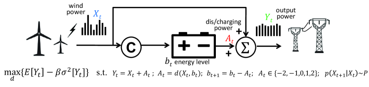
Figure 1: The control of renewable energy with storage systems without wind abandonment.

We apply Algorithm 1 to find the optimal control policy of the battery. Note that since the wind abandonment is not allowed, the long-run average output power $\mathbb{E}[Y_{t}]$ is not affected by actions. That is, the value of $\mathbb{E}[Y_{t}]$ is independent of policies and it is determined by the statistics of wind power. Therefore, this scheduling problem is a special case of our optimization problem (7) for mean-variance combined metrics and it satisfies the condition discussed in Remarks 2&4. The necessary condition in Theorem 2 is also a sufficient condition for this case and Algorithm 1 converges to the global optimum, as indicated by Remark 4. For demonstration, we choose $\beta=0.1$ and the optimization results are illustrated by Fig. 2. From Fig. 2, we can see that the variance $\sigma^{2}[Y_{t}]$ is continually reduced while $\mathbb{E}[Y_{t}]$ remains unvaried as 2.3605. The mean-variance combined metric $\mathbb{E}[Y_{t}]-\beta\sigma^{2}[Y_{t}]$ is continually improved until converged after 4 iterations and its optimum is 2.0826.

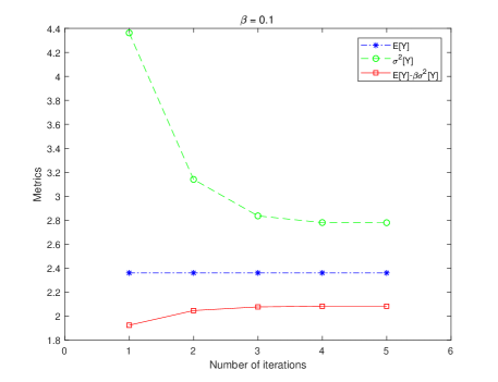
Figure 2: The convergence procedure of Algorithm 1 without wind abandonment.

Moreover, we randomly choose different initial policies and find that Algorithm 1 always converges to the same optimal policy, which is truly the global optimum. This is also consistent with the results in Remarks 2&4. The convergence results under some different initial policies are illustrated in Fig. 3, where different colors and notations indicate the convergence procedure from different initial policies. With Fig. 3, we can see that the algorithm converges to the same point with the minimal variance, i.e., $\sigma^{2}[Y_{t}]=2.7793$.

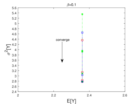
Figure 3: The same convergence point of Algorithm 1 under different initial policies, where Remarks 2&4 work.

To demonstrate the convergence efficiency of Algorithm 1, we further conduct an experiment of traditional gradient-based algorithm as a comparison. Since the control variable is the charging or discharging power, it is denoted as $a\in\mathcal{A}=\{-2,-1,0,1,2\}$. We use the randomized policy $\bm{\theta}$ such that the parameters can be updated with gradient-descent algorithms. With the performance derivative formula (34), we can compute the gradient $\frac{\mathrm{d}J_{\mu,\sigma}}{\mathrm{d}\theta_{i,a}}$ for each $a\in\mathcal{A}$ and each system state $i=(X_{t},b_{t})$, where $\theta_{i,a}$ is the probability of selecting action $a$ at state $i$. We first choose an arbitrary initial policy, say $\bm{\theta}_{i}=(0,0,1,0,0)$, i.e., the initial action is always $a=0$. At each state $i\in\mathcal{S}$, after computing the value of gradient $\frac{\mathrm{d}J_{\mu,\sigma}}{\mathrm{d}\theta_{i,a}}$, we find the action $a_{m}$ whose gradient is maximal. Then, we update the parameters as $\theta^{l+1}_{i,a_{m}}=\theta^{l}_{i,a_{m}}+\alpha_{l}$ and $\theta^{l+1}_{i,a}=\theta^{l}_{i,a}$ for all other $a\neq a_{m}$, where $\alpha_{l}$ is the step size at the $l$th iteration and we set it as a relatively large amount, say $\alpha_{l}=1/\sqrt{l}$. Then, we do normalization $\theta^{l+1}_{i,a}=\theta^{l+1}_{i,a}/\sum_{a\in\mathcal{A}}\theta^{l+1}_{i,a}$ such that the sum of $\bm{\theta}^{l+1}_{i}$ equals 1. We update the parameters $\bm{\theta}$ repeatedly until the difference of $\bm{\theta}$ between two successive iterations is smaller than a given threshold, say $0.1\%$ in ratio. The algorithm stops and outputs the current $\bm{\theta}^{*}$ as the optimal randomized policy. The experiment results are illustrated by Fig. 4.

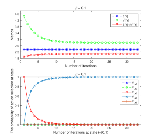
Figure 4: The experiment results of the gradient-based algorithm.

The two sub-figures in Fig. 4 illustrate the convergence curves of performance metrics and randomized parameters, respectively. Here we only choose $\bm{\theta}_{i}$ as an example, where $i=(0,1)$ means that the wind power is 0 and the battery energy level is 1. From Fig. 4 we can see that the gradient-descent algorithm converges after 33 iterations, although we choose a relatively large step size as $\alpha_{l}=1/\sqrt{l}$. At the convergence point, the performance metrics are $\mathbb{E}[Y_{t}]=2.3605$, $\sigma^{2}[Y_{t}]=2.7802$, and $\mathbb{E}[Y_{t}]-\beta\sigma^{2}[Y_{t}]=2.0825$, which are close to and slightly worse than our previous results of Algorithm 1. We can also see that the convergence speed of this gradient-based algorithm is much slower than that of our policy iteration type algorithm. Moreover, from the convergence curves of randomized parameters $\bm{\theta}_{i}$ in Fig. 4, we can see that $\bm{\theta}_{i}$ converges to a deterministic action $(0,0,0,1,0)$. It means that the optimal action is discharging the battery with power $a=1$ when the state is $i=(0,1)$, which looks reasonable. This also verifies the optimality of deterministic policies, as stated in Theorem 3.

5.2 Wind Abandonment Allowed

In this subsection, we study another scenario in which the wind abandonment is allowed. All the parameter settings are the same as those in the previous subsection. The difference is that we can abandon an extra power $V_{t}$ if necessary. In this scenario, we define the action as $U_{t}:=A_{t}-V_{t}$, where $0\leq V_{t}\leq X_{t}$. Variable $A_{t}$ has the same constraint as that in the previous subsection, i.e., $A_{t}\in\mathcal{A}$ and $b_{t}-B\leq A_{t}\leq b_{t}$. Although $A_{t}$ and $V_{t}$ are both variables, we can only use $U_{t}$ as the decision variable after using the following reasonable assumptions. If $0\leq U_{t}\leq\min\{\max(\mathcal{A}),\ b_{t}\}$, then we have $V_{t}=0$ and $A_{t}=U_{t}$, which means that the battery is discharging and the wind power should not be abandoned. If $\max\{\min(\mathcal{A}),\ b_{t}-B\}\leq U_{t}<0$, then we have $V_{t}=0$ and $A_{t}=U_{t}$, which means that the battery has potential charging capacity unused and the wind power should not be abandoned. If $-X_{t}\leq U_{t}<\max\{\min(\mathcal{A}),\ b_{t}-B\}$, then we have $V_{t}=A_{t}-U_{t}$ and $A_{t}=\max\{\min(\mathcal{A}),\ b_{t}-B\}$, which means that the battery is using full charging power capacity and some wind power is abandoned.

In summary, the value domain of the decision variable $U_{t}$ is $-X_{t}\leq U_{t}\leq\min\{\max(\mathcal{A}),\ b_{t}\}$ and it has the rule as follows: if $\max\{\min(\mathcal{A}),\ b_{t}-B\}\leq U_{t}\leq\min\{\max(\mathcal{A}),\ b_{t}\}$, then $V_{t}=0$ and $A_{t}=U_{t}$; if $-X_{t}\leq U_{t}<\max\{\min(\mathcal{A}),\ b_{t}-B\}$, then $V_{t}=A_{t}-U_{t}$ and $A_{t}=\max\{\min(\mathcal{A}),\ b_{t}-B\}$. Therefore, we only need to optimize the variable $U_{t}$. Variables $A_{t}$ and $V_{t}$ can be determined by the aforementioned rule. The control policy $d$ is a mapping from $(X_{t},b_{t})$ to $U_{t}$, i.e., $U_{t}=d(X_{t},b_{t})$. The output power of the system is determined by $Y_{t}=X_{t}+U_{t}$. Our goal is to find the optimal value of $U_{t}$ at every state $(X_{t},b_{t})$ such that the mean-variance combined metric $\mathbb{E}[Y_{t}]-\beta\sigma^{2}[Y_{t}]$ can be maximized. The control procedure of this problem is illustrated in Fig. 5.

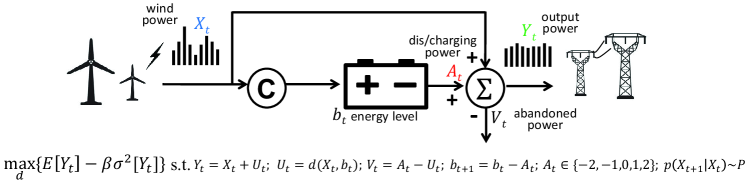
Figure 5: The control of renewable energy with storage systems with wind abandonment.

We use Algorithm 1 to maximize the mean-variance combined metric of this problem. We arbitrarily choose an initial policy from the policy space. For different initial policies, Algorithm 1 may converge to different local optima. Fig. 6 shows the convergence procedure when $\beta=0.5$. It can be observed that the variance of power output $\sigma^{2}[Y_{t}]$ is strictly reduced during each iteration, while the average power output $\mathbb{E}[Y_{t}]$ has an increasing trend. The combined metric $\mathbb{E}[Y_{t}]-\beta\sigma^{2}[Y_{t}]$ is continually improved after several iterations until Algorithm 1 converges. Algorithm 1 makes a balance between the wind abandonment and the fluctuation reduction, which demonstrates the effectiveness of Algorithm 1 for maximizing $\mathbb{E}[Y_{t}]-\beta\sigma^{2}[Y_{t}]$. It is also observed that Algorithm 1 converges after 5 to 7 iterations in most cases, which shows the fast convergence speed of Algorithm 1.

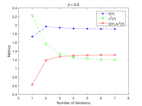
Figure 6: The convergence procedure of Algorithm 1 with wind abandonment.

Moreover, we investigate the convergence results of Algorithm 1 under different initial policies and different coefficients $\beta$. In each subgraph of Fig. 7, we randomly choose 5 different initial policies to implement Algorithm 1. Different curves indicate different convergence trajectories under different initial policies. For the case of $\beta=1$, we observe that Algorithm 1 converges to two different local optima; For other cases, different initial policies converge to the same local optimum. Every circle in Fig. 7 represents a feasible solution. We prefer the solutions with large $\mathbb{E}[Y_{t}]$ and small $\sigma^{2}[Y_{t}]$. Some of the feasible solutions are the Pareto solutions, which dominate other solutions in either $\mathbb{E}[Y_{t}]$ or $\sigma^{2}[Y_{t}]$. All the Pareto solutions form the Pareto frontier, which can be partly reflected in Fig. 7.

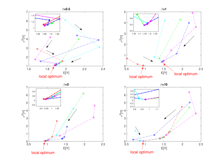
Figure 7: The convergence results of different initial policies and different $\beta$.

Note that the solution space is too large for us to enumerate every initial policies in Fig. 7. We only choose some representative solutions to outline the convergence procedures. The top-left corner of each subgraph is the zooming-in area around the convergence points. In future research, it is valuable to further apply the exploration mechanisms such that the algorithm has capability to jump out from local optima.

One intuitive way of exploration is to randomly sample the initial policy such that Algorithm 1 can start at different initial points and converge to different local optima. We can record the optimal policy best so far until the computation budget is depleted. In order to make the initial points as diverse as possible, we may define proper metrics to measure the diversity of a policy set. One example of heuristic ways to define the diversity metric of a policy set $\mathcal{D}_{0}\subseteq\mathcal{D}$ is as follows.

$$\Psi(\mathcal{D}_{0}):=\sum_{s\in\mathcal{S}}\Big{|}\bigcup_{d\in\mathcal{D}_{0}}d(s)\Big{|},$$ (40)

where $|\cdot|$ is the number of elements in the set and (40) means the sum of the numbers of different actions at all states. Thus, given the size of initial policy set $\mathcal{D}_{0}$, if $\mathcal{D}_{0}$ is more diverse, we expect that Algorithm 1 may converge to different local optima and the best one is more likely the global optimum.

Another intuitive way is to introduce exploration schemes during the step of policy generation in Algorithm 1. That is, we modify (36) such that the generated new policy can have more diversity. One feasible way is to use the $\epsilon$-greedy scheme which is widely adopted in reinforcement learning (Sutton and Barto, 2018). At each state $s$, we adopt the action determined by (36) with probability $1-\epsilon$ and randomly select actions from $\mathcal{A}$ with probability $\epsilon$, where $\epsilon$ is a small positive number such as $\epsilon=0.05$. We can record and output the best so far $J_{\mu,\sigma}$ until the computation budget is depleted. Another more effective way is to use the UCB (upper confident bound) method to balance the exploitation and exploration during the search procedure (Agrawal, 1995; Auer, 2002). We can define a counter $n(s,a)$ which records the number of pair $(s,a)$ evaluated during algorithm execution. We replace (36) with the following scheme

$$d^{(l+1)}(i):=\operatorname*{argmax}\limits_{a\in\mathcal{A}}\Bigg{\{}r(i,a)-\beta[r(i,a)-J_{\mu}]^{2}+\sum_{j\in\mathcal{S}}p^{a}(i,j)g_{\mu,\sigma}(j)+\gamma\sqrt{\frac{2\ln(\sum_{a}{n(s,a)})}{n(s,a)}}\Bigg{\}},$$

where the square root part reflects the exploration benefit and $\gamma$ is a coefficient balancing the exploitation and exploration. Such scheme is effective especially considering the estimation errors of $g_{\mu,\sigma}(j)$’s. We can let the coefficient $\gamma$ vanishing when the estimation of $g_{\mu,\sigma}(j)$ becomes more accurate. Similar schemes are widely used in sample-based optimization algorithms, such as Monte-Carlo tree search in AlphaGo (Silver et al., 2016) and adaptive sampling in MDPs (Chang et al., 2007). We can also resort to other exploration techniques such as local search and global search techniques widely used in evolutionary algorithms.

6 Discussion and Conclusion

The mean-variance combined metrics reflect both the average performance and the risk-related performance. Since the variance function is not additive, this mean-variance combined optimization problem does not fit the standard model of MDPs. The classical method of dynamic programming is not applicable. We study this problem from a new perspective called the theory of sensitivity-based optimization. The performance difference formula is established to directly quantify the difference of the mean-variance combined metrics under any two policies. The necessary condition of the optimal policy is derived. The optimality of deterministic policies is proved. We also develop a policy iteration type algorithm to optimize the mean-variance combined metric. The convergence of the algorithm is studied. Similar to the traditional policy gradient approach, our approach also converges to a local optimum in the mixed and randomized policy space, but with a more efficient way as it has a form of policy iteration. The global convergence of the algorithm is also discussed with the special condition in Remarks 2&4 or adopting some exploration and sampling techniques. Experiment examples of the fluctuation reduction of wind power with battery energy storage are conducted to demonstrate the effectiveness of our approach.

One of the future research topics is to implement our approach in a data-driven mode. This is a promising direction to study the risk-sensitive reinforcement learning algorithm, since the variance metric can reflect the risk-related factors. The online algorithm implementation and the integration with neural networks deserve further investigations, which is important to handle the issues of model-absence and the curse of dimensionality. Another future research topic is to extend our approach to optimize higher moment metrics or even distribution optimization, since the variance is only a second moment metric. For example, the third and the fourth moment of rewards are also interesting metrics in statistics, which reflect the skewness and kurtosis of reward distributions. One recent work makes a good initiate on the mean-variance-skewness-kurtosis analysis for the classic newsvendor problem in a static optimization regime (Zhang et al., 2020), while a more general study in a wider field and dynamic optimization regime will be a significant and challenging research topic.

References

- Altman (1999) Altman, E. Constrained Markov Decision Processes. Chapman and Hall, 1999.
- Agrawal (1995) Agrawal, R. (1995). Sample mean based index policies with O(log n) regret for the multi-armed bandit problem. Advances in Applied Probability 27, 1054-1078.
- Artzner et al. (1999) Artzner, P., Delbaen, F., Eber, J. M., Heath, D. (1999). Coherent measures of risk. Math. Finance 9, 203-228.
- Auer (2002) Auer, P. (2002). Using confidence bounds for exploitation-exploration trade-offs. Journal of Machine Learning Research 3, 397-422.
- Avi-Itzhak and Levy (2004) Avi-Itzhak, B. and Levy, H. (2004). On measuring fairness in queues. Advances in Applied Probability 36(3), 919-936.
- Bäuerle and Jaśkiewicz (2015) Bäuerle, N. and Jaśkiewicz, A. (2015). Risk-sensitive dividend problems. European Journal of Operations Research 242, 161-171.
- Bertsekas (2005) Bertsekas, D. P. (2005). Dynamic Programming and Optimal Control–Vol. I. Athena Scientific.
- Bertsekas and Tsitsiklis (1996) Bertsekas, D. P. and Tsitsiklis J. N. (1996). Neuro-Dynamic Programming. Athena Scientific, Belmont, Massachusetts.
- Borkar (2002) Borkar, V. (2002). Q-learning for risk-sensitive control. Mathematics of Operations Research 27, 294-311.
- Borkar (2010) Borkar, V. (2010). Learning algorithms for risk-sensitive control. Proceedings of the 19th International Symposium on Mathematical Theory of Networks and Systems (MTNS’2010), July 5-9, 2010, Budapest, Hungary, pp. 1327-1332.
- Cao (2007) Cao, X. R. (2007). Stochastic Learning and Optimization – A Sensitivity-Based Approach. New York: Springer.
- Cao and Zhang (2008) Cao, X. R. and Zhang, J. (2008). The nth-order bias optimality for multi-chain Markov decision processes. IEEE Transactions on Automatic Control 53, 496-508.
- Chang et al. (2007) Chang, H. S., Fu, M. C., Hu, J., and Marcus, S. I. (2007). Simulation-Based Algorithms for Markov Decision Processes. Springer.
- Chiu et al. (2018) Chiu, C. H., Choi, T. M., Dai, X., Shen, B., and Zheng, J. H. (2018). Optimal advertising budget allocation in luxury fashion markets with social influences: A mean-variance analysis. Production and Operations Management 27, 1611-1629.
- Chong and Zak (2013) Chong, E. K. P. and Zak, S. H. (2013). An Introduction to Optimization, 4th Edition. Wiley.
- Chow et al. (2015) Chow, L. M., Tamar, A., Mannor, S., and Pavone, M. (2015) Risk-sensitive and robust decision-making: a CVaR optimization approach. Proceedings of the 28th International Conference on Neural Information Processing Systems (ICML’2015), Montreal, Canada, December 07-12, 2015, pp. 1522-1530.
- Chung (1994) Chung, K. J. (1994). Mean-variance tradeoffs in an undiscounted MDP: the unichain case. Operations Research 42, 184-188.
- Delage and Mannor (2010) Delage, E. and Mannor, S. (2010). Percentile optimization for Markov decision processes with parameter uncertainty. Operations Research 58, 203-213.
- Feinberg and Schwartz (2002) Feinberg, E. and Schwartz, A. (2002). Handbook of Markov Decision Processes: Methods and Applications. Boston, MA: Kluwer Academic Publishers.
- Fu et al. (2009) Fu, M. C., Hong, L. J., and Hu, J. Q. (2009). Conditional Monte Carlo estimation of quantile sensitivities. Management Science 55 (12), 2019-2027.
- Gao et al. (2017) Gao, J., Zhou, K., Li, D., and Cao, X. R. (2017). Dynamic mean-LPM and mean-CVaR portfolio optimization in continuous time. SIAM Journal on Control and Optimization 55(3), 1377-1397.
- Guo and Zhang (2019) Guo, X. and Zhang, J. (2019). Risk-sensitive continuous-time Markov decision processes with unbounded rates and Borel spaces. Discrete Event Dynamic Systems: Theory and Applications 29(4), 445-471.
- Guo and Song (2009) Guo, X. and Song, X. Y. (2009). Mean-variance criteria for finite continuous-time Markov decision processes. IEEE Transactions on Automatic Control 54, 2151-2157.
- Guo et al. (2012) Guo, X., Ye, L., and Yin, G. (2012). A mean-variance optimization problem for discounted Markov decision processes. European Journal of Operational Research 220, 423-429.
- Haskell and Jain (2013) Haskell, W. B. and Jain, R. (2013). Stochastic dominance-constrained Markov decision processes. SIAM Journal on Control and Optimization 51(1), 273-303.
- Harrison and Qin (2009) Harrison, C. A. and Qin, S. J. (2009). Minimum variance performance map for constrained model predictive control. Journal of Process Control 19, 1199-1204.
- Hernandez-Lerma et al. (1999) Hernandez-Lerma, O., Vega-Amaya, O., and Carrasco, G. (1999). Sample-path optimality and variance-minimization of average cost Markov control processes. SIAM Journal on Control and Optimization 38, 79-93.
- Ho and Cao (1991) Ho, Y. C. and Cao, X. R. (1991). Perturbation Analysis of Discrete Event Dynamic Systems, Springer.
- Hong et al. (2014) Hong, L. J., Hu, Z., and Liu, G. (2014). Monte Carlo methods for value-at-risk and conditional value-at-risk: A review. ACM Transactions on Modeling and Computer Simulation 24, 1-37.
- Huang and Haskell (2017) Huang, W. and Haskell, W. B. (2017). Risk-aware Q-Learning for Markov decision processes. Proceedings of the 56th IEEE Conference on Decision and Control (CDC’2017), December 12-15, 2017, Melbourne, Australia, pp. 4928-4933.
- Huang (2018) Huang, Y. (2018). Finite horizon continuous-time Markov decision processes with mean and variance criteria. Discrete Event Dynamic Systems: Theory and Applications 28(4), 539-564.
- Huo et al. (2017) Huo, H., Zou, X., and Guo, X. (2017). The risk probability criterion for discounted continuous-time Markov decision processes. Discrete Event Dynamic Systems: Theory and Applications 27(4), 675-699.
- Kouvelis et al. (2018) Kouvelis, P., Pang, Z., and Ding, Q. (2018). Integrated commodity inventory management and financial hedging: A dynamic mean-variance analysis. Production and Operations Management 27(6), 1052-1073.
- Li et al. (2014) Li, Y. Z., Wu, Q. H., Li, M. S., Zhan, J. P. (2014). Mean-variance model for power system economic dispatch with wind power integrated. Energy 72, 510-520.
- Lim et al. (2013) Lim, S., Xu, H., and Mannor, S. (2013). Reinforcement learning in robust Markov decision processes. Proceedings of the NIPS’2013, Lake Tahoe, CA, The USA.
- Littman et al. (1995) Littman, M. L., Dean, T. L., and Kaelbling, L. P. (1995). On the complexity of solving Markov decision problems. Proceedings of the 11th Conference on Uncertainty in Artificial Intelligence, Morgan Kaufmann Publishers Inc.
- Luh et al. (2014) Luh, P. B., Yu, Y., Zhang, B., Litvinov, E., Zheng, T., Zhao, F., Zhao, J., and Wang, C. (2014). Grid integration of intermittent wind generation: A Markovian approach. IEEE Transactions on Smart Grid 5, 732-741.
- Markowitz (1952) Markowitz, H. (1952). Portfolio selection. The Journal of Finance 7, 77-91.
- Mannor and Tsitsiklis (2013) Mannor, S. and Tsitsiklis, J. N. (2013). Algorithmic aspects of mean-variance optimization in Markov decision processes. European Journal of Operational Research 231, 645-653.
- Nilim and El Ghaoui (2005) Nilim, A. and El Ghaoui, L. (2005). Robust control of Markov decision processes with uncertain transition matrices. Operations Research 53, 780-798.
- NREL (online) NREL. National wind technology center. [online]. Available on website http://www.nrel.gov/midc/nwtcm2.
- Parpas and Rustem (2007) Parpas, P. and Rustem, B. (2007). Computational assessment of nested benders and augmented lagrangian decomposition for mean-variance multistage stochastic problems. INFORMS Journal on Computing 19, 149-312.
- Powell (2007) Powell, W. B. (2007). Approximate Dynamic Programming: Solving the Curses of Dimensionality. John Wiley & Sons.
- Prashanth and Ghavamzadeh (2013) Prashanth, L. A. and Ghavamzadeh, M. (2013). Actor-critic algorithms for risk-sensitive MDPs. Proceedings of the 26th International Conference on Neural Information Processing Systems (NIPS’2013), 252-260.
- Puterman (1994) Puterman, M. L. (1994). Markov Decision Processes: Discrete Stochastic Dynamic Programming. New York: John Wiley & Sons.
- Ruszczyński (2010) Ruszczyński, A. (2010). Risk-averse dynamic programming for Markov decision processes. Mathematical Programming 125, 235-261.
- Ruszczyński and Shapiro (2006) Ruszczyński, A. and Shapiro, A. (2006). Conditional risk mappings. Mathematics of Operations Research 31, 544-561.
- Schulman et al. (2015) Schulman, J., Levine, S., Moritz, P., Jordan, M., and Abbeel, P. (2015). “Trust region policy optimization,” Proceedings of the 31st International Conference on Machine Learning (ICML’2015), Lille, France, pp. 1889-1897.
- Shapiro (2009) Shapiro, A. (2009). On a time consistency concept in risk averse multistage stochastic programming. Oper. Res. Lett. 37, 143-147.
- Silver et al. (2016) Silver, D., Huang, A., Maddison, C. J., Guez, A., Sifre, L., and Van, D. G. (2016). Mastering the game of go with deep neural networks and tree search. Nature 529(7587), 484-489.
- Sobel (1994) Sobel, M. J. (1994). Mean-variance tradeoffs in an undiscounted MDP. Operations Research 42, 175-183.
- Sutton and Barto (2018) Sutton, R. S. and Barto, A. G. (2018). Reinforcement Learning: An Introduction, 2nd Edition. MIT Press, Cambridge, MA.
- Tamar et al. (2012) Tamar, A., Castro, D. D., and Mannor, S. (2012). Policy gradients with variance related risk criteria. Proceedings of the 29th International Conference on Machine Learning (ICML’2012), Edinburgh, Scotland.
- Tamar et al. (2013) Tamar, A., Castro, D. D., and Mannor, S. (2013). Temporal difference methods for the variance of the reward to go. Proceedings of the 13rd International Conference on Machine Learning (ICML’2013), pp. 495-503.
- Xia (2016) Xia, L. (2016). Optimization of Markov decision processes under the variance criterion. Automatica 73, 269-278.
- Xia (2018a) Xia, L. (2018a). Mean-variance optimization of discrete time discounted Markov decision processes. Automatica 88, 76-82.
- Xia (2018b) Xia, L. (2018b). Variance minimization of parameterized Markov decision processes. Discrete Event Dynamic Systems: Theory and Applications 28, 63-81.
- Xia et al. (2014) Xia, L., Jia, Q. S., and Cao, X. R. (2014). A tutorial on event-based optimization – A new optimization framework. Discrete Event Dynamic Systems: Theory and Applications 24(2), 103-132.
- Xia and Yang (2019) Xia, L. and Yang, Z. (2019). A new method for mean-variance optimization of stochastic dynamic systems. Proceedings of the 2019 IEEE Conference on Control Technology and Applications (CCTA’2019), August 19-21, 2019, Hong Kong, pp. 856-859.
- Yang et al. (2018) Yang, Z., Xia, L., and Guan, X. (2018). Fluctuation reduction of wind power with battery energy storage systems. Proceedings of the 2018 IEEE International Conference on Automation Science and Engineering (CASE’2018), August 20-23, 2018, Munich, Germany, pp. 762-767.
- Yu et al. (2017) Yu, P., Haskell, W. B., and Xu, H. (2017). Approximate value iteration for risk-aware Markov decision processes. IEEE Transactions on Automatic Control 63(9), 3135-3142.
- Zhang et al. (2020) Zhang, J., Sethi, S. P., Choi, T. M., and Cheng, T. C. E. (2020). Supply chains involving a mean-variance-skewness-kurtosis newsvendor: Analysis and coordination. Production and Operations Management 29(6), 1397-1430.
- Zhou and Li (2000) Zhou, X. Y. and Li, D. (2000). Continuous-time mean-variance portfolio selection: a stochastic LQ framework. Applied Mathematics & Optimization 42, 19-33.
- Zhou and Yin (2004) Zhou, X. Y. and Yin, G. (2004). Markowitz’s mean-variance portfolio selection with regime switching: A continuous-time model. SIAM Journal on Control and Optimization 42, 1466-1482.