Consistent High Dimensional Rounding with Side Information

Abstract

In standard rounding, we want to map each value $X$ in a large continuous space (e.g., $\mathbb{R}$) to a nearby point $P$ from a discrete subset (e.g., $\mathbb{Z}$). This process seems to be inherently discontinuous in the sense that two consecutive noisy measurements $X_{1}$ and $X_{2}$ of the same value may be extremely close to each other and yet they can be rounded to different points $P_{1}\neq P_{2}$, which is undesirable in many applications. In this paper we show how to make the rounding process perfectly continuous in the sense that it maps any pair of sufficiently close measurements to the same point. We call such a process consistent rounding, and make it possible by allowing a small amount of information about the first measurement $X_{1}$ to be unidirectionally communicated to and used by the rounding process of the second measurement $X_{2}$. In many applications such as the creation of a biometric database of fingerprints, we can naturally use such a scheme by storing in each entry the user’s identity, a hashed version of the initial measurement of his fingerprints, and the side information which will enable any future noisy reading of the fingerprint to be consistently hashed to the same value.

The fault tolerance of a consistent rounding scheme is defined by the maximum distance between pairs of measurements which guarantees that they will always be rounded to the same point, and the goal of this paper is to study the possible tradeoffs between the amount of information provided and the achievable fault tolerance for various types of spaces. When the measurements $X_{i}$ are arbitrary vectors in $\mathbb{R}^{d}$, we show that communicating $\log_{2}(d+1)$ bits of information is both sufficient and necessary (in the worst case) in order to achieve consistent rounding for some positive fault tolerance, and when d=3 we obtain a tight upper and lower asymptotic bound of $(0.561+o(1))k^{1/3}$ on the achievable fault tolerance when we reveal $\log_{2}(k)$ bits of information about how $X_{1}$ was rounded. We analyze the problem by considering the possible colored tilings of the space with $k$ available colors, and obtain our upper and lower bounds with a variety of mathematical techniques including isoperimetric inequalities, the Brunn-Minkowski theorem, sphere packing bounds, and Čech cohomology.

1 Introduction

Rounding.

Whenever we want to digitally process or store an analog value, we have to perform some kind of rounding in order to represent this value (which is typically a number in $\mathbb{R}$) by a nearby point chosen from a discrete subset (such as the set of integers $\mathbb{Z}$). In the multidimensional generalization of this problem we are given a vector $X\in\mathbb{R}^{d}$, and want to represent it by a nearby point $P$ chosen from some discrete subset of $\mathbb{R}^{d}$ (which may be $\mathbb{Z}^{d}$, some lattice of points, or any other choice). Many rounding procedures had been proposed and studied in the literature (see, e.g., [2, 8]), but all of them are inherently discontinuous in the sense that one can always find two inputs which are extremely close to each other (such as $0.49999$ and $0.50001$) which are mapped to different outputs (such as $0$ and $1$). In fact, any such rounding scheme partitions the space into a disjoint union of bounded subsets called tiles, in which each tile is rounded to a different representative point (e.g., its center), and the discontinuities happen along the tiles’ boundaries. The algorithmic aspect of the problem of actually finding the tile that contains a given $X$ in a given partition is a classical problem in computational geometry, and had been studied extensively under the general name of point location (see [9, 18], and the references therein).

In many applications, such discontinuities are undesirable. One natural solution is to try to minimize the fraction of pairs $X_{1},X_{2}$ with $distance(X_{1},X_{2})<\epsilon$ which are mapped to different tiles by considering foam tilings that minimize the total surface area of unit volume tiles (such a tiling is called ‘foam’ since it emerges automatically in physical collections of soap bubbles). In a beautiful FOCS’2008 paper [16] (which later appeared as a research highlight at CACM [17]), Kindler, Rao, O’Donnell and Wigderson introduced a clever new construction of such tiles which they called spherical cubes. What makes these tiles special is that they have the $O(\sqrt{d})$ surface area of a ball and yet they can tile the whole $\mathbb{R}^{d}$ space without gaps. Surprisingly, the main motivation for this construction came from the seemingly unrelated field of computational hardness amplification, and it solved an interesting open problem posed by Lord Kelvin in $1887$.

A related class of schemes that aim at minimizing the proportion of close points mapped to different places is locality sensitive hashing schemes (see, e.g., [14]). However, they typically deal with situations in which the input is a vector and the output is a scalar, and thus they do not actually round inputs to nearby outputs in the same space.

Our approach – consistent rounding.

In this paper we consider the more ambitious goal of completely eliminating all the discontinuities in the rounding process rather than reducing their fraction. We call any such scheme consistent rounding. To make it possible, we have to slightly modify the model by thinking about $X_{1}$ and $X_{2}$ as two consecutive noisy measurements of the same $X$. When the first measurement $X_{1}$ is rounded, we allow it to produce a few bits of side information about how it was rounded and to provide them as an auxiliary input to the process that decides how to round $X_{2}$.

The one-dimensional case. To demonstrate the basic idea, consider the one dimensional case in which $X_{1}$ and $X_{2}$ are real values which have to be consistently rounded to a nearby integer. $X_{1}$ is always rounded to the nearest integer, and it produces a single bit of side information which is whether it was rounded to an even or odd integer $P$. When $X_{2}$ is measured, it is rounded to the nearest integer which is of the same parity as $P$. To demonstrate this process, consider again the problematic inputs $X_{1}=0.49999$ and $X_{2}=0.50001$: $X_{1}$ is rounded to $0$, and $X_{2}$ is also rounded to $0$ since it is the closest even integer. In fact, $X_{2}$ could be anywhere between $-1$ and $1$ and still be consistently rounded to $0$, and thus the rounding scheme can tolerate any additive fault up to $0.5$. It is not difficult to show (see Section 4.1.1) that this is the highest possible fault tolerance of any one dimensional consistent rounding scheme, and that other natural schemes (such as providing one bit of side information about whether $X_{1}$ was rounded up or down) provide lower fault tolerance.

The way we think about the problem is to consider a colored tiling of the real line with two colors: All the values in $[-0.5,0.5)$ are colored by 1, all the values in $[0.5,1.5)$ are colored by 2, all the values in $[1.5,2.5)$ are colored by 1, all the values in $[2.5,3.5)$ are colored by 2, etc. The side information provided about $X_{1}$ is the color of the tile in which it is located, and the way we process $X_{2}$ is to round it to the center of the closest tile which has the same color as that of $X_{1}$. The essential property of our partition is that the minimum distance between any two tiles which have the same color is $1$, and thus we can “inflate” all the tiles of a particular color to include any erroneously measured value $X_{2}$ up to a distance of $0.5$ away from the original tile, and still get nonoverlapping tiles which make it possible to uniquely associate such points with original tiles. This is reminiscent of how error correcting codes operate: To guarantee unique decoding, we “inflate” each codeword into a ball around it, and demand that all these balls will be disjoint. The error correction bound is thus half of the distance between the two closest codewords. The main difference is that in our case we inflate tiles rather than points, and try to maximize the smallest distance between tiles that have the same color (for each color separately).

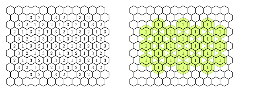
Figure 1: A 3-colored hexagonal tiling of the plane, and a maximal non-intersecting inflation of the tiles colored 1

The two-dimensional case. To make this perspective clearer, consider the two dimensional plane. If we use the obvious checkerboard tiling by unit squares, we need at least 4 colors (and thus 2 bits of side information) to color the tiles if we want any two tiles with the same color to have some positive distance between them. We can reduce the number of colors to 3 (and thus, provide only $\log_{2}(3)=1.58$ bits of side information) by considering the hexagonal partition of the plane depicted in the left part of Figure 1. Given a two dimensional point $X_{1}$, we always round it to the center of the hexagon in which it is located, and given $X_{2}$ we round it to the center of the nearest hexagon which has the same color as the hexagon that contains $X_{1}$. To determine the fault tolerance of this consistent rounding scheme, we inflate all the hexagonal tiles of a particular color by the same amount until two of them touch each other for the first time, as depicted in the right part of Figure 1. As it turns out, this scheme is not optimal: even though the hexagonal partition is very attractive since its circle-like tiles map each point to a nearby center, when we inflate the hexagons of a particular color we are stopped prematurely when their corners touch, leaving large gaps between the inflated hexagons. A 3-colored tiling with a higher fault tolerance will be described in Section 4.2.1, and an asymptotically optimal tiling for a large number of colors will be described in Section 4.2.2.

A fine point about consistent rounding schemes is how to break ties, and here we deal differently with $X_{1}$ and $X_{2}$. We want to be able to deal with any $X_{1}$, and thus we think about the tiles as being closed sets which include their boundaries. Therefore, points $X_{1}$ which are on the boundary between tiles can have more than one possible color. We allow such ties to be broken arbitrarily in the sense that $X_{1}$ can be rounded to the center of any one of the tiles that it belong to. However, when we think about $X_{2}$ we allow it to be at a distance of strictly less than some bound, and thus the inflated tiles (that contain all the possible $X_{2}$’s we are interested in) are open sets which have no intersections. Consequently, each $X_{2}$ can belong to at most one inflated tile, and is rounded to the center of that tile with no possible ties.

The minimal amount of side information that allows high-dimensional consistent rounding.

When we consider higher dimensional inputs $X\in\mathbb{R}^{d}$, we can provide one bit of side information about each one of its $d$ entries separately, but for large $d$ this requires a large number of side information bits. In our colored tiling formulation of the problem, it suffices to reveal the color of $X_{1}$ in order to consistently round $X_{2}$, and thus if we tile the space with $k$ colors, we need only $\log_{2}(k)$ bits of side information to specify this color. This naturally leads to the question of what is the minimum number of colors needed to tile $\mathbb{R}^{d}$ by bounded sized tiles so that all the tiles of the same color will have some positive distance from each other (note that two colors always suffice if we relax the problem by allowing an infinite series of nested boxes, or allow tiles of the same color to touch at corners). Surprisingly, we could not find in the literature any reference to this natural question. As we show in Section 3, there can be no such colored tiling with $d$ colors, and as we show in Section 5.2.1, $d+1$ colors are sufficient. Consequently, $\log_{2}(d+1)$ bits of side information about $X_{1}$ are necessary and sufficient (in the worst case) in order to obtain a consistent rounding scheme with positive fault tolerance. To prove the negative result, we use techniques borrowed from algebraic topology (namely, the Čech cohomology and other cohomology theories), and to prove the positive result we provide an explicit construction of such a colored tiling.

The maximal fault tolerance that can be achieved with a given amount of side information.

In addition to aiming at minimizing the amount of side information, we study the question of maximizing the fault tolerance for a given amount of side information. In Section 4 we study the special case of the two dimensional plane. In the negative direction, we obtain several upper bounds on the fault tolerance that can be achieved, using different techniques from geometry and analysis (including isoperimetry, the Brunn-Minkowski inequality and results on the circle packing problem). In the positive direction, we construct a variety of tiling schemes for various numbers of colors. In particular, while for three colors the hexagonal tiling scheme described above can tolerate an additive fault of up to $0.31$, we present a tiling with fault tolerance of $0.354$, and show that no 3-color tiling can have fault tolerance higher than $0.413$. When the number $k$ of colors tends to infinity, we derive the asymptotic bound of $(0.537+o(1))\sqrt{k}$ on the achievable fault tolerance, and prove its tightness by an explicit construction.

In Section 5 we study the general case of $\mathbb{R}^{d}$, $d>2$. Like in the two-dimensional case, we obtain a number of lower and upper bounds on the fault tolerance. In particular, we show that the maximal fault tolerance achieved by a $(d+1)$-coloring of $\mathbb{R}^{d}$ is between $\Omega(1/d)$ and $O(\log d/\sqrt{d})$. In addition, we use the recent breakthrough results on the sphere packing problem [5, 13, 19] to obtain tight asymptotic lower and upper bounds on the fault tolerance in dimensions $3,8,$ and $24$. Our bounds on fault tolerance are summarized in Table 1.

Scenario	Lower Bound	Upper Bound	Techniques	Source
	(LB) on FT	(UB) on FT
3 colors	0.354	0.413	Brunn-Minkowski ineq. (UB),	Sec. 4.1.1 (UB),
in $\mathbb{R}^{2}$			Brick wall const. (LB)	Sec. 4.2.1 (LB)
4 colors	0.5	0.564	Brunn-Minkowski ineq. (UB),	Sec. 4.1.1 (UB),
in $\mathbb{R}^{2}$			Brick wall const. (LB)	Sec. 4.2.1 (LB)
$k$ colors	$(0.537+o(1))\sqrt{k}$	$(0.537+o(1))\sqrt{k}$	Circle packing (UB),	Sec. 4.1.2 (UB),
in $\mathbb{R}^{2}$			HCR const. (LB)	Sec. 4.2.2 (LB)
4 colors	0.175	0.365	Brunn-Minkowski ineq. (UB),	Sec. 5.1.1 (UB),
in $\mathbb{R}^{3}$			Bricks and balloons const. (LB)	Sec. 5.2.2 (LB)
$d+1$ colors	$\Omega(1/d)$	$O(\log d/\sqrt{d})$	Brunn-Minkowski ineq. (UB),	Sec. 5.1.1 (UB),
in $\mathbb{R}^{d}$			Dimension reducing const. (LB)	Sec. 5.2.1 (LB)
$k$ colors	$(0.561+o(1))k^{1/3}$	$(0.561+o(1))k^{1/3}$	Sphere packing (UB),	Sec. 5.1.2 (UB),
in $\mathbb{R}^{3}$			CPB const. (LB)	Sec. 5.2.3 (LB)
$k$ colors	$(0.707+o(1))k^{1/8}$	$(0.707+o(1))k^{1/8}$	Sphere packing (UB),	Sec. 5.1.2 (UB),
in $\mathbb{R}^{8}$			CPB const. (LB)	Sec. 5.2.3 (LB)
$k$ colors	$(1+o(1))k^{1/24}$	$(1+o(1))k^{1/24}$	Sphere packing (UB),	Sec. 5.1.2 (UB),
in $\mathbb{R}^{24}$			CPB const. (LB)	Sec. 5.2.3 (LB)
FT – fault tolerance, LB – lower bound, UB – upper bound, Const. – construction
HCR – honeycomb of rectangles, CPB – close packing of boxes

Table 1: Summary of our lower and upper bounds on the fault tolerance, for different values of the dimension $d$ and the number of colors $k$

Applications.

The problem of consistent rounding has numerous applications. For example, consider the problem of biometric identification, in which multiple measurements of the same fingerprint are similar but not identical. It would be very helpful if all these slight variants could be represented by the same rounded point $P$, and we can achieve this by storing a small amount of side information in the biometric database (as part of the initial acquisition of the biometric data of a new employee).

Another example is the problem of developing a contact tracing app for the COVID-19 pandemic, where we want to record all the cases in which two smart phones were at roughly the same place at roughly the same time. We can do this by measuring in each phone the GPS location, the local time, and perhaps other parameters such as the ambient noise level or the existence of sudden accelerations (to determine that the two phones were in the same moving car). When someone tests positive for COVID-19, the health authority can release a list of his measurements, but in order to keep the patient’s privacy, it wants to apply a cryptographically strong hash function to each measurement before publishing it. Since we expect these measurements to be slightly different for the infected and exposed persons, the health authority can publish the small amount of side information along with the consistently rounded and then hashed measurements.

Finally, in industrial control systems we can collect analog measurements from thousands of sensors (temperature, pressure, flow, etc.) and the use of a consistent rounding scheme could be ideal in order to check the repeatability of the process in spite of slight variations.

Related work.

A line of study that seems related to our work is fuzzy constructions that were widely studied in the cryptographic literature. For example, [10] introduces the notions of fuzzy extractors and secure sketches, which enable two parties to secretly reach a consensus value from multiple noisy measurements of some high entropy source (a recent survey of such techniques can be found in [12]). However, such schemes concentrate on the aspects of cryptographic security (which we do not consider), and produce sketches whose size depends on the number of possible inputs (which is meaningless for real valued inputs). In this sense our consistent rounding scheme can be viewed as an exceptionally efficient reconciliation process, since it can produce for each million entry vector of arbitrarily large real numbers a $20$ bit “sketch” (in the form of its color side information), and process this information with trivial point location algorithms.

An actual application in which side information is used during an “error reconciliation” process can be found in the post quantum key exchange scheme New Hope by Alkim et.al. [1]. Their approach is limited to lattice points, and requires side information whose size is linear in the number of dimensions, while our approach requires only a logarithmic number of bits.

Another natural idea (which is used in many fuzzy cryptographic constructions such as fuzzy commitment [15]) is to use an error correction scheme to map inputs to nearby codewords. However, most error correction schemes cannot be applied to real valued inputs. In addition, even if we could perfectly tile the continuous input space with balls surrounding each codeword, this would not solve the problem of consistent rounding near the boundary between adjacent balls. Finally, this boundary problem becomes worse as the dimension grows, since in high dimensions almost all the points are likely to be near a boundary. Consequently, these code based cryptographic solutions manage to solve a variety of interesting related tasks, but not the consistent rounding problem we consider in this paper.

Open problems.

While we fully solved the question of minimizing the amount of side information required for fault tolerance, several questions remain open regarding the maximal tolerance rate that can be achieved for a given amount of side information. In particular, for dimensions $2,3,8,24$ we determined the exact asymptotic fault tolerance rate when $\log_{2}k$ bits of information are allowed, using a connection to the densest sphere packing problem. When only very few bits of information are allowed, the situation is much less clear. For example, we do not even know whether the brick wall constructions we present in Section 4.2.1 have the highest fault tolerance among rounding schemes in $\mathbb{R}^{2}$ with $\log_{2}3$ and $\log_{2}4$ bits of side information. It will be interesting to obtain new upper bounds via different techniques or new lower bound constructions.

2 Our Setting

In this section we present the basic setting that will be assumed throughout the paper.

Tiling.

We study tilings of $\mathbb{R}^{d}$, where each tile is connected, closed and bounded, and the tiles intersect only in their boundaries. We further assume that the tiling is locally finite, meaning that the number of tiles that intersect any bounded ball $B(0,r)$ is finite. In some of the results we make additional assumptions on the tiles; such assumptions are stated explicitly.

Coloring.

In our tiling, each tile is colored in one of $k$ colors. We note that the natural assumption that the tiles are unicolored is made for the sake of simplicity; all our results hold also if the tiles contain several colors, provided that the color classes inside each tile satisfy the assumptions we made on the tiles.

Fault tolerance and inflation.

In order to compute the fault tolerance of a given tiling (with respect to the $L_{2}$ distance), we consider all tiles of the same color and inflate them (i.e., replace the tile $T$ by the set $T^{\prime}=\{y:\exists x\in T,|x-y|<r\}$ for some $r>0$) until they touch each other. Clearly, the fault tolerance is the maximal $r$ for which such a non-intersecting inflation is possible.

We denote the minimal distance between two same-colored points in different tiles by $t$, and so, the fault tolerance is $t/2$.

Normalization.

The $d$-dimensional volume of a figure $T\subset\mathbb{R}^{d}$ is denoted by $\lambda(T)$. We normalize the tiling by assuming that the volume of each tile is bounded by $1$ (like in the 1-dimensional case presented in the introduction, where all tiles are segments of length $1$). We make the natural assumption that any inflated tile $T^{\prime}$ satisfies $\lambda(\bar{T}^{\prime})=\lambda(T^{\prime})$, where $\bar{T}^{\prime}$ is the closure of $T^{\prime}$.

We choose this normalization since it complies with using the Brunn-Minkowski theorem (see Section 4.1.1) and makes computations more convenient. We note that our results can be easily translated to results with respect to other natural normalizations. For example, the assumption that the radius of each tile is at most $1$ (which means that the $L_{2}$ distance between each $X\in\mathbb{R}^{d}$ and its rounded value is at most $1$) implies that the volume of each tile is at most the volume of the unit ball in $\mathbb{R}^{d}$, which allows translating all our fault tolerance upper bounds to this ‘bounded radius’ setting. As for the lower bounds, they come from explicit constructions whose fault tolerance can be recomputed with respect to any other natural normalization.

Alternative metrics.

Instead of the $L_{2}$ distance (which is probably the most natural distance metric), one may consider the fault tolerance problem with respect to other distance metrics.

For example, in order to measure the fault tolerance with respect to the $L_{\infty}$ distance, one has to inflate each tile $T$ into $T^{\prime\prime}=\{y:\exists x\in T,\max_{i}|x_{i}-y_{i}|<r\}$. It turns out that the problem is much easier with respect to this metric. Indeed, assume that the number of colors is $k=m^{d}$ for some $2\leq m\in\mathbb{N}$. Consider a periodic tiling in which each basic unit is a cube with side length $m$ that consists of $m^{d}$ unit-cube tiles, each colored in a different color. This tiling achieves fault tolerance of $(m-1)/2$. On the other hand, it is easy to see that the argument via the Brunn-Minkowski theorem presented in Section 4.1.1 implies that any tiling of $\mathbb{R}^{d}$ with $k=m^{d}$ colors achieves fault tolerance of at most $(m-1)/2$ with respect to the $L_{\infty}$ metric, and thus, the cubic tiling we described is optimal. Lower and upper bounds for other values of $k$ can be obtained by variants of this construction and the corresponding upper bound proof.

The difference between the metrics comes from the fact that in ‘cubic’ inflation (which is done with respect to the $L_{\infty}$ metric), non-intersecting inflations of cubic tiles fill the entire space, while in inflation by balls (which we have with respect to the $L_{2}$ metric), large gaps are left between the inflated tiles.

3 The Minimal Number of Colors Required for Fault Tolerance

In this section we prove that the minimal number of colors required for tolerating any rate $t>0$ of faults in a tiling of $\mathbb{R}^{d}$ is $d+1$. We provide two proofs, under different additional natural assumptions on the tiles. The first proof assumes that the tiles are polytopes and uses an inductive argument. The second proof assumes that the tiles and their non-empty intersections are contractible and uses an algebraic-topologic argument. The lower bound $d+1$ on the number of required colors is tight; a matching construction for any $d$ is presented in Section 5.2.1.

3.1 Lower bound for polytopic tiles

In this section we prove the following.

Proposition 3.1

For any $m>0$, the following holds. Let $T_{1},T_{2},\ldots$ be a colored tiling of $\mathbb{R}^{d}$ in which the tiles are polytopes and each tile is contained in a box with side length $m$. If the fault tolerance of the tiling is $>0$, then the number of colors is at least $d+1$.

Informal proof.

We show by induction that there is a point $x$ that is included in at least $d+1$ tiles. This implies that if the tiling uses only $d$ colors, there must be two same-colored tiles that intersect in $x$, and thus, no fault tolerance is possible.

For $d=1$, as each single tile is included in a segment of length $m$, for any $M>m$, the entire segment $[-M,M]$ cannot be covered by a single tile. Hence, the segment must contain a point in which two tiles intersect.

For the induction step, we consider the restriction of the tiling to a large box $[-M,M]^{d}$. Then we look at the $d$’th coordinate, consider the union of all tiles that contain a point in the ‘lower’ half-box, and take the ‘upper boundary’ of this union. This gives a ‘crumpled’ variant of the equator hyperplane. By the induction hypothesis, the restriction of the tiling to this ‘crumpled hyperplane’ contains a point $v$ that is included in at least $d$ tiles. However, there is also at least one tile in the ‘upper half-box’ that includes $v$, and thus, $v$ is included in at least $d+1$ tiles. This completes the proof by induction.

Formal proof.

Making the argument described above formal is somewhat cumbersome, and requires an auxiliary notion, somewhat close to the notion of a polytopal complex [21, p. 127].

Notation.

Let $k,d,m,M\in\mathbb{N}$, be such that $d\geq k$ and $M>m$. A crumpled $(k,d)$-flat $F$ is a union of a finite collection of $k$-dimensional polytopes $P_{1},P_{2},\ldots,P_{\ell}\in\mathbb{R}^{d}$ that satisfies the following conditions:

1. $F$ is contained in the slab $[-M,M]^{k}\times[0,m]^{d-k}$.

2. The projection of $F$ onto the hyperplane $H_{k}=\mathbb{R}^{k}\times\{0\}^{d-k}$ is $[-M,M]^{k}\times\{0\}^{d-k}$.

3. $F$ is connected.

4. Each $P_{i}$ is contained in a box with side length $m$.

5. The intersection of any $P_{i},P_{j}\in F$ is either empty or a polytope of dimension $\leq k-1$.

Figure 2: An illustration of the inductive process of Lemma 3.2. A polygonal tiling of $[-3,3]^{2}$ is depicted in ordinary lines, and the ‘crumpled equator’ to which we reduce in the inductive process (that has to be included in the slab $[-3,3]\times[0,2]$ and whose projection on the $x$-axis must be $[-3,3]$) is depicted by a bold line. The bold line is a crumpled $(1,2)$-flat with the parameters $M=3,m=2$.

For example, a crumpled $(1,d)$-flat is a polygonal line included in the slab $[-M,M]\times[0,m]^{d-1}$, whose projection on the $x$-axis is $[-M,M]$. A crumpled $(1,2)$-flat with the parameters $M=3,m=2$ is demonstrated in Figure 2 (in boldface).

Lemma 3.2

Let $k,d,m,M$ be as above. Any crumpled $(k,d)$-flat $F$ contains a point that belongs to at least $k+1$ polytopes.

Proof: The proof goes by induction on $k$. For $k=1$, observe that $F$ cannot consist of a single polytope. Indeed, as the projection of $F$ on the $x$-axis is $[-M,M]$, there are two points $v,v^{\prime}\in F$ with $|v-v^{\prime}|\geq 2M$. These points cannot belong to the same polytope $P_{i}$, since each $P_{i}$ is included in a segment of length $m$. As $F$ is connected, it must contain an intersection point of two $P_{i}$’s.

For the induction step, consider a crumpled $(k,d)$-flat $F$. Let $F^{\prime}$ be the union of all polytopes in $F$ whose intersection with the set $\{x\in\mathbb{R}^{d}:x_{k}\leq 0\}$ is non-empty, and let

$$F^{\prime\prime}=\partial(F^{\prime})\cap\{x\in\mathbb{R}^{d}:x_{k}\geq 0\}.$$

(That is, we look at the $k$’th coordinate and take to $F^{\prime}$ all polytopes in $F$ that contain a point in the ‘lower’ half-space. Then, we define $F^{\prime\prime}$ to be the intersection of the boundary of $F^{\prime}$ with the ‘upper’ half-space. We view $F^{\prime\prime}$ as a ‘crumpled equator flat’ of $F$). This process, in the case $d=2$, $k=1$, is demonstrated in Figure 2, where the tiling $F$ is depicted in ordinary lines and $F^{\prime\prime}$ is depicted by a bold line.

We view $F^{\prime\prime}$ as the union of the polytopes $P^{\prime}_{i}=P_{i}\cap F^{\prime\prime}$. We claim that $F^{\prime\prime}$ is a crumpled $(k-1,d)$-flat. Indeed:

1. $F^{\prime\prime}$ is contained in the slab $[-M,M]^{k-1}\times[0,m]^{d-k+1}$, since each $v\in\partial(F^{\prime})$ belongs to some $P_{i}$ that contains also a point $v^{\prime}$ with $v^{\prime}_{k}\leq 0$. As each $P_{i}$ is included in a box of side length $m$, we have $v^{\prime}_{k}\leq m$. (The condition in all other coordinates clearly holds.)

2. For any fixed value $(x_{1},\ldots,x_{k-1})\in[-M,M]^{k-1}$, the projection of the set $\{v\in F:(v_{1},\ldots,v_{k-1})=(x_{1},\ldots,x_{k-1})\}$ on the $k$’th axis is $[-M,M]$. In particular, $F^{\prime}$ contains a point whose first $k$ coordinates are $(x_{1},\ldots,x_{k-1},0)$. We can take such a point, and move from it in the positive direction of the $k$’th axis until we reach a point on the boundary of $F^{\prime}$. The resulting point is an element in $F^{\prime\prime}$ whose first $k-1$ coordinates are $x_{1},\ldots,x_{k-1}$. Hence, the projection of $F^{\prime\prime}$ on $H_{k-1}$ is $[-M,M]^{k-1}\times\{0\}^{d-k+1}$.

3. $F^{\prime}$ is connected, and hence, $F^{\prime\prime}=\partial(F^{\prime})\cap\{x\in\mathbb{R}^{d}:x_{k}\geq 0\}$ is connected as well.

4. Each polytope in $F^{\prime\prime}$ is contained in a box of side length $m$, since it is part of a polytope that was contained in $F^{\prime}$.

5. The intersection of any $P^{\prime}_{i},P^{\prime}_{j}\in F^{\prime\prime}$ is either empty or a polytope, since $P^{\prime}_{i},P^{\prime}_{j}$ are parts of faces of polytopes (from $F$) created by intersection with other polytopes or with the halfspace $\{x\in\mathbb{R}^{d}:x_{k}\geq 0\}$. The dimension of any such intersection is at most $k-2$ since the transformation from $H^{\prime}$ to its boundary reduces all dimensions by 1.

By the induction hypothesis, $H^{\prime\prime}$ contains an intersection point $v$ of $k$ polytopes $P^{\prime}_{i}$. This means that the corresponding polytopes $P_{i}$ contain $v$ as well.

Furthermore, as $v\in\partial(H^{\prime})$ and $0\leq v_{k}\leq m$, there exists $P_{j}\in H\setminus H^{\prime}$ that contains $v$. (Here, we use the assumption that for any sufficiently small $\epsilon>0$, $H$ contains some $w$ with $(w_{1},\ldots,w_{k})=(v_{1},\ldots,v_{k-1},v_{k}+\epsilon)$ and the assumption that $F$ consists of a finite collection of polytopes.) Therefore, $v$ belongs to at least $k+1$ polytopes of $H$, completing the proof by induction. $\Box$

Now we are ready to prove Proposition 3.1.

Proof: Let $T_{1},T_{2},\ldots$ be a tiling of $\mathbb{R}^{d}$ that satisfies the assumptions of the proposition. Let $T^{\prime}_{i}=T_{i}\cap[-M,M]^{d}$, and let $F=\cup T^{\prime}_{i}$. It is easy to see that $F$ is a crumpled $(d,d)$-flat. Hence, by the lemma, $F$ contains a point $v$ that belongs to $d+1$ polytopes. The point $v$ is included in at least $d+1$ tiles $T_{i}$, proving the assertion. $\Box$

Remark.

We note that if one assumes that the tiles are convex polytopes, then a much simpler argument shows that at least $d+1$ colors are needed. Indeed, start with a point in some tile, and move in some direction until you reach the boundary of the tile. The points on this boundary belong to two tiles. Move along this boundary face until you reach a point on its boundary (i.e., now we reduce from dimension $d-1$ to $d-2$.) The points on this boundary already belong to at least three tiles. We can continue reducing dimension, until we reach dimension $0$ with a point that belongs to $d+1$ tiles. This argument fails in nonconvex polytopes since the corners of a box nested inside a bigger box touch only two tiles.

3.2 Lower bound for contractible tiles

Recall that a set in $\mathbb{R}^{d}$ is called contractible if is can be continuously shrunk to a point in $\mathbb{R}^{d}$. (The formal definition is that the identity map is homotopic to some constant map.)

Informally, in this section we prove that if the tiles and their non-empty intersections are finite unions of contractible sets, then at least $d+1$ colors are required for fault tolerance. Due to the possibility of pathologies, the formal statement is a bit more cumbersome:

Proposition 3.3

Let $T_{1},T_{2},\ldots$ be a colored tiling of $\mathbb{R}^{d}$ in which the tiles and all their non-empty intersections are disjoint unions of finitely many contractible sets. Assume that the tiling is locally finite and that all $T_{i}$’s are bounded. In addition, assume that each $T_{i}$ has an open neighborhood $U_{i}$ such that for any set of indices $I,$

$$\bigcap_{i\in I}U_{i}\neq\emptyset\Leftrightarrow\bigcap_{i\in I}T_{i}\neq\emptyset,$$

and the $U_{i}$’s and their non-empty intersections are disjoint unions of finitely many contractibles.

Then the number of colors is at least $d+1$.

A similar method proves an analogous statement for colored tilings of the sphere $\mathbb{S}^{d}$:

Proposition 3.4

Let $T_{1},T_{2},\ldots,T_{N}$ be a colored tiling of $\mathbb{S}^{d}$ in which the tiles and all their non-empty intersections are disjoint unions of finitely many contractible sets. Assume that each $T_{i}$ has an open neighborhood $U_{i}$ such that for any set of indices $I,$

$$\bigcap_{i\in I}U_{i}\neq\emptyset\Leftrightarrow\bigcap_{i\in I}T_{i}\neq\emptyset,$$

and the $U_{i}$’s and their non-empty intersections are disjoint unions of finitely many contractibles.

Then the number of colors is at least $d+1$.

Remark 3.5

We stress that for most natural tilings the additional assumption on the existence of the neighborhoods $U_{i}$ follows from the existence of $T_{i}$’s with the corresponding properties. However, there are topological pathologies in which this is not the case.

The proof of Propositions 3.3 and 3.4 uses the notion of Čech cohomology and classical results regarding its properties. For the ease of reading, we begin with an intuitive explanation of the proof ideas, and then present the formal proof.

Intuitive proof.

The $d$’th (singular) cohomology group is a topological invariant of a manifold which roughly counts “non trivial holes” of dimension $d$. A classical result asserts that the $d$’th cohomology group of a $d$-dimensional compact oriented manifold like $\mathbb{S}^{d}$ is $\mathbb{R}$. (This corresponds to the intuitive understanding that $\mathbb{S}^{d}$ has one $d$-dimensional hole.) The de-Rham cohomology and the Čech cohomology are analytic and algebro-geometric/combinatorial invariants, that in many cases agree with their topological cousin. In particular, the $d$’th de-Rham and Čech cohomologies of $\mathbb{S}^{d}$ are equal to $\mathbb{R}$ as well.

The $d$’th Čech cohomology with respect to an open cover of the manifold depends on properties of intersections of $d+1$ sets in that cover. In general, it depends on the sets which form the cover, however, it is known that if these sets and their non-empty intersections are finite disjoint unions of contractibles, then the cohomology groups remain the same, independently of the cover. In particular, if the $d$’th Čech cohomology with respect to such a cover is non trivial, then there must be $d+1$ sets with a non-empty intersection.

Hence, for our cover $U_{1},U_{2},\ldots$, we know that its $d$’th Čech cohomology is $\mathbb{R}$. This readily completes the proof of the proposition for $\mathbb{S}^{d}$, as this implies that there must be a point that belongs to at least $d+1$ of the $U_{i}$’s.

The proof in $\mathbb{R}^{d}$ works in essentially the same way, with cohomology groups replaced by cohomology groups with compact support.

Formal proof.

For the proof we recall the notion of Čech cohomology with values in the constant sheaf $\underline{\mathbb{R}}$, and describe the slightly less standard concept of Čech cohomology with compact support.

Definitions.

Let $S$ be either $\mathbb{R}^{d}$ or a compact manifold such as $\mathbb{S}^{d}.$ Let $\mathcal{U}=\{U_{1},U_{2},\ldots\}$ be an open cover of $S.$ If $S$ is compact, we assume the collection to be finite. If $S$ is $\mathbb{R}^{d}$, we assume it to be locally finite and assume in addition that each $U_{i}$ is bounded.

• A $q-$simplex $\sigma=\{U_{i_{0}},\ldots,U_{i_{k}}\}$ of ${\mathcal{U}}$ is an ordered collection of $q+1$ different sets chosen from $\mathcal{U},$ such that

  $$\bigcap_{k=0}^{q}U_{i_{k}}\neq\emptyset.$$

• For a $q-$simplex $\sigma=(U_{i_{k}})_{k\in\{0,\ldots,q\}}$, the $j$’th partial boundary is the $(q-1)$-simplex

  $$\partial_{j}\sigma:=(U_{i_{k}})_{k\in\{0,\ldots,q\}\setminus\{j\}},$$

  obtained by removing the $j$’th set from $\sigma$.

• A $q-$cochain of $\mathcal{U}$ is a function which associates to any $q-$simplex a real number. The $q-$cochains form a vector space denoted by $C^{q}(\mathcal{U},\underline{\mathbb{R}}),$ with operations

  $$(\lambda f+\mu g)(\sigma)=\lambda f(\sigma)+\mu g(\sigma),\quad\mbox{where}\quad\lambda,\mu\in\mathbb{R},~{}f,g\in C^{q}(\mathcal{U},\underline{\mathbb{R}}),~{}\sigma~{}\mbox{ is a $q-$simplex}.$$

  Similarly, we define $C^{q}_{c}(\mathcal{U},\underline{\mathbb{R}}),$ as the vector space of $q-$cochains with compact support, meaning those cochains which assign $0$ to all $q-$simplices, except for finitely many.

• There is a differential map $\delta_{q}:C^{q}(\mathcal{U},\underline{\mathbb{R}})\to C^{q+1}(\mathcal{U},\underline{\mathbb{R}})$ whose application to $f\in C^{q}(\mathcal{U},\underline{\mathbb{R}})$ is the $(q+1)-$cochain $\delta_{q}(f)$ whose value at a $(q+1)-$simplex $\sigma$ is

  $$(\delta_{q}f)(\sigma)=\sum_{j=0}^{q+1}(-1)^{j}f(\partial_{j}\sigma).$$

  The restriction of $\delta_{q}$ to $C^{q}_{c}(\mathcal{U},\underline{\mathbb{R}})$ maps it to $C^{q+1}_{c}(\mathcal{U},\underline{\mathbb{R}})$.

• It can be easily seen that

  $$\delta_{q+1}\circ\delta_{q}=0.$$

• The $q$’th Čech cohomology group (with compact support) of $S$ with respect to the cover $\mathcal{U}$ and values in $\underline{\mathbb{R}}$ is

  $$\check{{H}}^{q}(\mathcal{U},\underline{\mathbb{R}}):=\mbox{Ker}(\delta_{q})/\mbox{Image}(\delta_{q-1}),$$

  $$(\check{{H}}^{q}_{c}(\mathcal{U},\underline{\mathbb{R}}):=\mbox{Ker}(\delta_{q}|_{C^{q}_{c}(\mathcal{U},\underline{\mathbb{R}})})/\mbox{Image}(\delta_{q-1}|_{C^{q-1}_{c}(\mathcal{U},\underline{\mathbb{R}})})).$$

• A cover (by open sets) is good if all its sets as well as their multiple intersections are either empty or contractible. It is almost good if all non empty intersections are unions of finitely many disjoint contractible components.

Classical results we use.

The first result we use is the following:

Theorem 3.6

If $S$ is a compact smooth orientable manifold (such as $\mathbb{S}^{d}$), and $\mathcal{U}$ is a good or an almost good finite cover, then

$$\check{H}^{i}(\mathcal{U},\underline{\mathbb{R}})\simeq{H}^{i}_{dR}(S),$$

where the right hand side is the standard de-Rham cohomology group.

Similarly, if $S=\mathbb{R}^{d}$ and $\mathcal{U}$ is a locally finite good or almost good cover whose sets are bounded, then

$$\check{H}^{i}_{c}(\mathcal{U},\underline{\mathbb{R}})\simeq{H}^{i}_{dR,c}(S),$$

where the right hand side is the $i$’th de-Rham cohomology group with compact support.

For further reading about de-Rham cohomology, with or without compact support, we refer the reader to [4, Sec. 1]. For further reading about the Čech cohomology, we refer to [4, Sec. 8]. In particular, Theorem 3.6, for the compact case and good covers is Theorem 8.9 there. The passage to almost good covers is straightforward: In the paragraph which precedes the proof, it is explained that the obstructions to the isomorphism between Čech and de-Rham cohomologies are given by products of the $i$’th de-Rham cohomology groups, for $i\geq 1,$ of the different intersections $\bigcap_{k=0}^{q}U_{i_{k}}.$ Since those intersections are disjoint unions of contractibles, their higher cohomology groups vanish, hence there is no obstruction to the isomorphism.

Regarding the case $S=\mathbb{R}^{d},$ the proof in [4, Sec. 8] requires a few small changes: In the statement of Proposition 8.5 there, one needs to replace the de-Rham complex of the manifold with the de-Rham complex with compact support, and the direct product with direct sum. The maps $r,\delta$ which appear there will still be well defined by our local finiteness assumption on the cover, and the assumption that $U_{i}$’s are bounded. The proof requires no change. Then, the double complex in the definition of Proposition 8.8 should also be defined using direct sum rather than direct product, but again there is no change in the proof. Given these changes in definitions, the proof of Theorem 8.9 (also for the almost good case) is unchanged.

The second standard result, which is a consequence of Poincaré duality, is the following:

Theorem 3.7

For a compact smooth oriented manifold $S$ of dimension $d$ (such as $\mathbb{S}^{d}$),

$${{H}}^{d}_{dR}(S)\simeq\mathbb{R}.$$

Similarly, for $S=\mathbb{R}^{d},$

$${H}^{d}_{dR,c}(\mathbb{R}^{d})\simeq\mathbb{R}.$$

See, for example, [4, Sec. 7] for the compact case, and [4, Sec. 4] for $\mathbb{R}^{d}.$

Theorems 3.6 and 3.7 yield:

Corollary 3.8

If $S$ is a compact smooth orientable manifold (such as $\mathbb{S}^{d}$), and $\mathcal{U}$ is a good or an almost good finite cover, then

$$\check{{H}}^{d}(\mathcal{U},\underline{\mathbb{R}})=\mathbb{R}.$$

Similarly, if $S=\mathbb{R}^{d}$ and $\mathcal{U}$ is a locally finite good or almost good cover whose sets are bounded, then

$$\check{{H}}^{d}_{c}(\mathcal{U},\underline{\mathbb{R}})=\mathbb{R}.$$

Proof of Propositions 3.3 and 3.4.

We show that there must exist $d+1$ $T_{i}$’s whose intersection is non-empty. This clearly implies that for any fault tolerance, at least $d+1$ colors are needed.

Assume on the contrary that any $(d+1)$-intersection of the $T_{i}$’s is empty. Let $U_{i}$ be as in the statement of the theorem. Then by definition, they form an almost good cover. All intersections of at least $d+1$ $U_{i}$’s are empty by our assumptions. Therefore, there are no $d-$simplices, and so $C^{d}(\mathcal{U},\underline{\mathbb{R}})=0.$ Thus, in the compact case, $\check{{H}}^{d}(\mathcal{U},\underline{\mathbb{R}})=0.$ But on the other hand, by Corollary 3.8,

$$\check{{H}}^{d}(\mathcal{U},\underline{\mathbb{R}})\simeq\mathbb{R},$$

a contradiction. In the case of $\mathbb{R}^{d}$ the same argument works, with $\check{{H}}^{d}_{c}(\mathcal{U},\underline{\mathbb{R}})$ in place of $\check{{H}}^{d}(\mathcal{U},\underline{\mathbb{R}})$.

4 Fault-Tolerant Rounding in the Plane

In this section we consider tilings of the plane by tiles $T_{1},T_{2},\ldots$ of area at most $1$. Each point in the plane is colored in one of $k\geq 3$ colors, and our goal is to maximize the minimal distance $t$ between two points of the same color that belong to different tiles. (The maximum is taken over all possible tilings that satisfy the mild regularity conditions stated in Section 2 and over all possible colorings.) Clearly, the fault tolerance of a rounding scheme based on such a colored tiling is $t/2$.

We present three upper bounds on $t$, using the Brunn-Minkowski inequality, the circle packing problem, and the Minkowski-Steiner formula, respectively. In the other direction, we prove lower bounds on $t$ by a series of explicit tilings. In particular, we obtain a tight asymptotic estimate for $t$, namely, $t=(\beta+o(1))\sqrt{k}$, where $\beta=\sqrt{2/\sqrt{3}}\approx 1.074$. Our main upper and lower bounds are summarized in Table 1.

4.1 Upper bounds on the fault tolerance

The basic idea behind our upper bound proofs is as follows. Assume we have a colored tiling of the plane, with minimal distance $t$. Pick a single color – say, black – and consider all black tiles inside a large square $S$. We obtain a new collection of tiles $T^{\prime}_{1},T^{\prime}_{2},\ldots,T^{\prime}_{m}$ that covers part of $S$. Now, the assumption that the minimal distance between two same-colored points in different tiles is $t$ implies that if we inflate each black tile $T^{\prime}_{i}$ into the set

$$T^{\prime\prime}_{i}=\{x:\exists y\in T^{\prime}_{i},|x-y|<t/2\},$$ (1)

then the inflations $T^{\prime\prime}_{i}$ are pairwise disjoint. Hence, the sum of their areas essentially cannot exceed the area of the large square, and this allows bounding $t$ from above.

4.1.1 An upper bound using the Brunn-Minkowski inequality

The inflations $T^{\prime\prime}_{i}$ have a convenient representation in terms of the Minkowski sum of sets in $\mathbb{R}^{2}$.

Definition 4.1

For two sets $A,B\subset\mathbb{R}^{d}$, the Minkowski sum of $A,B$ is $A+B=\{a+b:a\in A,b\in B\}$.

In terms of this definition, we have

$$T^{\prime\prime}_{i}=T^{\prime}_{i}+B(0,t/2),$$ (2)

where $B(0,t/2)$ is a disk of radius $t/2$ around the origin. This allows us to lower bound the area of each $T^{\prime\prime}_{i}$, using the classical Brunn-Minkowski (BM) inequality (see, e.g., [3]). Recall the inequality asserts the following.

Theorem 4.2 (Brunn-Minkowski)

Let $A,B$ be compact sets in $\mathbb{R}^{d}$. Then

$$\lambda(A+B)^{1/d}\geq\lambda(A)^{1/d}+\lambda(B)^{1/d},$$

where $\lambda(X)$ is the volume of $X$ (formally, the $d$-dimensional Lebesgue measure of $X$).

The inequality is tight if and only if $A,B$ are positive homothetic, i.e., are equal up to translation and dilation by a positive factor.

Proposition 4.3

Let $T_{1},T_{2},\ldots$ be a $k$-colored tiling of the plane, with tiles of area $\leq 1$ and minimal distance $t$. Then

$$t\leq\left(\frac{2}{\sqrt{\pi}}+o(1)\right)\cdot(\sqrt{k}-1)\approx 1.128(\sqrt{k}-1).$$

Proof: Consider a square $S$ such that $\lambda(S)=n^{2}$ (for some ‘large’ $n$). By the pigeonhole principle, there exists a color (say, black) that covers at least $n^{2}/k$ of the area of $S$. Look at the black tiles whose intersection with $S$ is non-empty, and denote their intersections with $S$ by $T^{\prime}_{1},T^{\prime}_{2},\ldots,T^{\prime}_{m}$. Hence, we have $m$ ‘black’ subsets of $S$, each of area at most 1, whose total area is at least $n^{2}/k$.

For each $T^{\prime}_{i}$, define $T^{\prime\prime}_{i}=T^{\prime}_{i}+B(0,t/2)$. By assumption, the regions $T^{\prime\prime}_{i}$ are disjoint. Furthermore, they are included in $S+B(0,t/2)$ whose area is less than $(n+t)^{2}$. By taking a sufficiently large $n$, we may assume

$$\sum_{i}\lambda(T^{\prime\prime}_{i})\leq(1+o(1))n^{2}.$$ (3)

By the Brunn-Minkowski inequality, we have

$$\forall i:\sqrt{\lambda(T^{\prime\prime}_{i})}\geq\sqrt{\lambda(T^{\prime}_{i})}+\sqrt{\pi}\cdot\frac{t}{2},$$

and thus,

$$\forall i:\lambda(T^{\prime\prime}_{i})\geq\lambda(T^{\prime}_{i})+\sqrt{\pi}\cdot t\cdot\sqrt{\lambda(T^{\prime}_{i})}+\pi t^{2}/4.$$

Summing over $i$ and using (3), we get

$$(1+o(1))n^{2}\geq\sum_{i=1}^{m}\lambda(T^{\prime\prime}_{i})\geq\sum_{i=1}^{m}\lambda(T^{\prime}_{i})+\sqrt{\pi}\cdot t\cdot\sum_{i=1}^{m}\sqrt{\lambda(T^{\prime}_{i})}+m\pi t^{2}/4.$$ (4)

Note that we have $\sum_{i}\lambda(T^{\prime}_{i})\geq n^{2}/k$ (by assumption), $\sum_{i}\sqrt{\lambda(T^{\prime}_{i})}\geq n^{2}/k$ (since $\forall 0\leq x\leq 1:\sqrt{x}\geq x$), and $m\geq n^{2}/k$ (since $\forall i:\lambda(T^{\prime}_{i})\leq 1$). Hence, we get

$$(1+o(1))n^{2}\geq\frac{n^{2}}{k}\cdot(1+\sqrt{\pi}\cdot t+\pi t^{2}/4)=\frac{n^{2}}{k}\cdot(1+\sqrt{\pi}t/2)^{2}.$$

Dividing by $n^{2}$ and rearranging, we get $(1+o(1))(\sqrt{k}-1)\geq\sqrt{\pi}t/2$, and hence,

$$t\geq\left(\frac{2}{\sqrt{\pi}}+o(1)\right)\cdot(\sqrt{k}-1)\approx 1.128(\sqrt{k}-1),$$

as asserted. $\Box$

Discussion.

Substituting specific values of $k$, the upper bounds that follow from Proposition 4.3 are $t\leq 0.826$ for $k=3$, $t\leq 1.128$ for $k=4$ and $t\leq 1.128\sqrt{k}$ for a large $k$.

These upper bounds are lossy in two ways. One source of loss is the application of the Brunn-Minkowski inequality. Here, the inequality is tight if the tiles are disks, and the farther they are from disks, the larger is the loss. Another source of loss is the space left between the inflations, that is not taken into account in the proof.

Interestingly, there is a dichotomy between these two sources of loss. As follows from the circle packing problem, when the tiles are disks (and so, there is no loss in the BM inequality), the space between the inflations (and so, the loss of the second type) is relatively large. The space between the inflations can be made smaller if the tiles are taken to be polygons with a few vertices. However, this comes at the expense of increased loss in the BM inequality, as is demonstrated in Section 4.1.3.

Optimality of our 1-dimensional rounding scheme.

The argument described above gives an easy proof of the optimality of the 1-dimensional rounding scheme presented in the introduction. Indeed, consider a 2-colored tiling of the line and look at the segment $I=[-n,n]$ for some large $n$. By the pigeonhole principle, we may assume that black tiles cover at least half of $I$. By the 1-dimensional Brunn-Minkowski inequality, for each black tile $T^{\prime}_{i}\subset I$ and the corresponding inflation $T^{\prime\prime}_{i}=T^{\prime}_{i}+(-t/2,t/2)$, we have $\lambda(T^{\prime\prime}_{i})\geq\lambda(T^{\prime}_{i})+t$. As $\forall i:\lambda(T^{\prime}_{i})\leq 1$, there are at least $n$ tiles. Since the $T^{\prime\prime}_{i}$’s are pairwise disjoint and included in $[-n-1,n+1]$, we obtain

$$2n+2\geq\sum_{i}\lambda(T^{\prime\prime}_{i})\geq\sum_{i}\lambda(T^{\prime}_{i})+\sum_{i}t\geq n+nt,$$

and thus, $t\leq(n+2)/n$. By letting $n$ tend to infinity, we obtain $t\leq 1$, implying that the fault tolerance of any two-colored tiling of the line is at most $1/2$.

4.1.2 An upper bound using the Circle Packing problem

This upper bound is interesting mainly for a large number $k$ of colors, where the size and form of the original tiles is negligible with respect to the size of the inflations. In this setting, we can represent each tile by a single point from it, and consider our problem as an instance of the well-known circle packing problem (see, e.g., [7]), as we know that circles of radius $t/2$ around the points must be disjoint. We use the following classical result of Fejes-Tóth [11]:

Theorem 4.4 (Fejes-Tóth)

The maximal number of points that can be placed in a square of area $a$, such that the minimal distance between two points is $1$, is at most $2a/\sqrt{3}$.

By rescaling, the theorem implies:

Corollary 4.5

The maximal number of points that can be placed in a square of area $a$, such that the minimal distance between two points is $t$, is at most $\frac{2a}{\sqrt{3}t^{2}}$.

Proposition 4.6

Let $T_{1},T_{2},\ldots$ be a tiling of the plane in $k$ colors, with tiles of area $\leq 1$ and minimal distance $t$. Then

$$t\leq\left(\sqrt{\frac{2}{\sqrt{3}}}+o(1)\right)\cdot\sqrt{k}\approx 1.074\sqrt{k}.$$

Proof: Like in the proof of Proposition 4.3, we begin with a tiling $T_{1},T_{2},\ldots$ with minimal distance $t$, consider the intersection with a square $S$ of area $n^{2}$, pick a single color (say, black) whose intersection with $S$ has area of at least $n^{2}/k$, and obtain disjoint black tiles $T^{\prime}_{1},\ldots,T^{\prime}_{m}$ inside a square $S$ of area $(1+o(1))n^{2}$, whose total area is at least $n^{2}/k$. We pick a single point $x_{i}$ from each tile $T^{\prime}_{i}$. By assumption, the minimal distance between the $x_{i}$’s is at least $t$. By Corollary 4.5, this implies

$$m\leq(1+o(1))\cdot\frac{2n^{2}}{\sqrt{3}t^{2}}.$$

On the other hand, $m\geq n^{2}/k$, since the total area of the black tiles is at least $n^{2}/k$ and the area of each tile is at most $1$. Therefore,

$$\frac{n^{2}}{k}\leq(1+o(1))\cdot\frac{2n^{2}}{\sqrt{3}t^{2}},$$

and consequently, $t\leq\left(\sqrt{\frac{2}{\sqrt{3}}}+o(1)\right)\cdot\sqrt{k}$, as asserted. $\Box$

Discussion.

For small values of $k$, this upper bound is rather weak – e.g., for $k=3$ we obtain $t\leq 1.861$ (compared to $t\leq 0.826$ via the BM inequality). This happens, since we completely neglect the tiles and consider only the area added in the inflation process. For a large $k$, when the area is dominated by the inflation step, the upper bound $t\leq(1.074+o(1))\sqrt{k}$ is tight, as will be shown in Section 4.2.2.

4.1.3 An upper bound using the Minkowski-Steiner formula

This upper bound is applicable under the additional condition that the tiles $T_{i}$ are convex. It uses another well-known result, called the Minkowski-Steiner formula.

Theorem 4.7 (Minkowski-Steiner)

Let $A$ be a convex compact set in $\mathbb{R}^{2}$. Then for any circle $B(0,r)$,

$$\lambda(A+B(0,r))=\lambda(A)+\ell(\partial A)r+\pi r^{2},$$ (5)

where $\ell(\partial(A))$ is the (1-dimensional) length of the boundary of $A$.

By substituting (5) into the proof of Proposition 4.3, we obtain

$$(1+o(1))n^{2}\geq\sum_{i=1}^{m}\lambda(T^{\prime\prime}_{i})=\sum_{i=1}^{m}\lambda(T^{\prime}_{i})+\frac{t}{2}\cdot\sum_{i=1}^{m}\ell(\partial(T^{\prime}_{i}))+m\pi t^{2}/4.$$ (6)

To proceed, we may bound the length of the boundary of each $T^{\prime}_{i}$ in terms of the area $\lambda(T^{\prime}_{i})$. If we do not make further assumptions on the $T^{\prime}_{i}$’s, then the best possible bound of this type is the isoperimetric inequality, which asserts

$$\ell(\partial(A))\geq\sqrt{4\pi}\sqrt{\lambda(A)},$$

for any region $A$ in the plane bounded by a closed curve. Plugging this into (6) yields exactly the same upper bound as Proposition 4.3 (which comes by no surprize, as the tightness case of the isoperimetric inequality is circles, just like the tightness case in the proof of Proposition 4.3).

However, if we further assume that each tile is a convex polygon, then we can obtain an improved bound, as function of the number of vertices in each such polygon. We use another classical result, going back to an Ancient Greec mathematician:

Theorem 4.8 (Zenodorus)

Among all polygons on $n$ vertices with the same area, the perimeter is minimized for the regular $n$-gon.

Recall that the perimeter of a regular $l$-gon $P_{l}$ of area $\lambda(P_{l})$ is

$$\ell(\partial(P_{l}))=\frac{2\sqrt{l}}{\sqrt{\cot(\pi/l)}}\cdot\sqrt{\lambda(P_{l})}.$$

Plugging this into (6), we obtain the following.

Proposition 4.9

Let $T_{1},T_{2},\ldots$ be a tiling of the plane in $k$ colors, with tiles of area $\leq 1$ and minimal distance $t$. Assume than all tiles are convex polygons with at most $l$ vertices. Then

$$t\leq(1+o(1))\cdot\frac{-\alpha_{l}+\sqrt{\alpha_{l}^{2}-4(1-k)\pi}}{\pi},\qquad\mbox{where}\qquad\alpha_{l}=\frac{2\sqrt{l}}{\sqrt{\cot(\pi/l)}}.$$

Proof: First, we follow the proof sketch presented above until Equation (6), which asserts

$$(1+o(1))n^{2}\geq\sum_{i=1}^{m}\lambda(T^{\prime\prime}_{i})=\sum_{i=1}^{m}\lambda(T^{\prime}_{i})+\frac{t}{2}\cdot\sum_{i=1}^{m}\ell(\partial(T^{\prime}_{i}))+m\pi t^{2}/4.$$

Using the theorem of Zenodorus, we obtain

$$(1+o(1))n^{2}\geq\sum_{i=1}^{m}\lambda(T^{\prime}_{i})+\frac{t}{2}\cdot\alpha_{l}\cdot\sum_{i=1}^{m}\sqrt{\lambda(T^{\prime}_{i})}+m\pi t^{2}/4,$$

where $\alpha_{l}=\frac{2\sqrt{l}}{\sqrt{\cot(\pi/l)}}$. As $m\geq n^{2}/k$ and $\sum_{i}\sqrt{\lambda(T^{\prime}_{i})}\geq\sum_{i}\lambda(T^{\prime}_{i})\geq n^{2}/k$, this implies

$$(1+o(1))n^{2}\geq\frac{n^{2}}{k}\cdot\left(1+\frac{t}{2}\cdot\alpha_{l}+\pi t^{2}/4\right),$$

and consequently, $(1+o(1))k\geq 1+\frac{\alpha_{l}}{2}t+\frac{\pi}{4}t^{2}$. Solving the quadratic inequality, we obtain

$$t\leq(1+o(1))\cdot\frac{-\alpha_{l}+\sqrt{\alpha_{l}^{2}-4(1-k)\pi}}{\pi},$$

as asserted. $\Box$

Discussion.

For small values of $l$, the upper bound obtained in Proposition 4.9 is rather strong. For example, for $l=3$ we obtain $t\leq 0.707$ for 3 colors and $t\leq 0.985$ for four colors. As the constructions we obtain below, based on rectangular tiles, satisfy $t=1/\sqrt{2}$ for 3 colors and $t=1$ for four colors, Proposition 4.9 shows that these constructions cannot be improved using triangular tiles.

As $l$ increases, the bound of Proposition 4.9 becomes weaker and approaches the bound of Proposition 4.3, since circles (for which Proposition 4.3 is tight) can be approximated to any precision by convex polygons with a sufficiently large number of vertices.

4.2 Lower bounds on the fault tolerance

In this subsection we present two series of explicit tilings. The first series provides the best lower bounds on $t$ for a small number of colors we aware of, and the second series shows the tightness of the asymptotic upper bound $t\leq(1.074+o(1))\sqrt{k}$.

4.2.1 The brick wall construction

In the brick wall construction with $k$ colors, demonstrated in Figure 3, each tile is a rectangle with side lengths $\sqrt{(k-2)/2}$ and $\sqrt{2/(k-2)}$ (and so, the area of each tile is $1$). The construction is periodic, where the basic unit is two rows of adjacent rectangles, colored in a round robin fashion. For an even $k$, the second row is placed exactly below the first row, and the sequence of colors is shifted by $k/2$. For an odd $k$, the second row is indented by half a brick (making the construction look like a brick wall), and the sequence of colors is shifted by $(k+1)/2$.

Figure 3: The brick wall construction for $k=3,4,5$ colors. The ratio between the width and the height of each tile is $2:k-2$.

It is easy to see that the minimal distance between two same-colored points in different tiles is $\sqrt{(k-2)/2}$. (This distance is attained both in the vertical and in the horizontal directions. Having the same minimal distance in both directions is the optimization that dictates the side lengths of the bricks.)

In particular, we obtain the lower bounds $t\geq 1/\sqrt{2}$ for 3 colors, $t\geq 1$ for 4 colors, and $t\geq\sqrt{3/2}$ for 5 colors.

4.2.2 The honeycomb of rectangles construction

In the honeycomb of rectangles construction with $k=m^{2}$ colors, each tile is a rectangle with side lengths $a$ and $1/a$, where

$$a=\left(\frac{m^{2}-2m+1}{\frac{3}{4}m^{2}-m}\right)^{1/4}.$$ (7)

The construction is periodic, where the basic unit is composed as follows. First, we construct a basic ‘large rectangle’, which is an $m$-by-$m$ square block of tiles, using all the $k=m^{2}$ colors (in arbitrary order). Then, the basic unit of the construction is two ‘fat rows’ of adjacent large rectangles, where the second row is indented by half a large rectangle. The coloring of each large rectangle is the same. The construction, for $k=16$, is demonstrated in Figure 4.

Figure 4: The honeycomb of rectangles construction for $k=16$ colors. The boundaries of the basic ‘large rectangles’ are depicted in bold. The placement of the tiles in each single color corresponds to the honeycomb lattice.

Note that the set of tiles colored in some single color forms the shape of a honeycomb lattice (including the centers of the hexagons). This is why we call the construction ‘honeycomb of rectangles’.

It is easy to see that the minimal horizontal and diagonal distances between two same-colored tiles are

$$(m-1)a\qquad\mbox{and}\qquad\sqrt{\left(\frac{m-1}{a}\right)^{2}+\left(\left(\frac{m}{2}-1\right)a\right)^{2}},$$

respectively. By choosing $a$ such that the two distances are equal, we obtain (7), and the asymptotic lower bound

$$t\geq(1+o(1))\left(\frac{4}{3}\right)^{1/4}\cdot m\approx 1.074\sqrt{k},$$

that matches the upper bound obtained above.

5 Fault-Tolerant Rounding in Higher Dimensions

In this section we consider tilings of $\mathbb{R}^{d}$, for $d\geq 3$, by tiles $T_{1},T_{2},\ldots$ of volume at most $1$. As was shown in Section 3, the minimal number of colors that allows for any fault tolerance is $d+1$.

First, we obtain two upper bounds on the fault tolerance, by generalizing the bounds via the Brunn-Minkowski inequality and via the circle packing problem presented in Section 4.1. In the other direction, we present an explicit tiling with $d+1$ colors that attains a minimal distance of $t=\frac{1}{1+2(d-1)\sqrt{2}}$ (and hence, fault tolerance of $t/2$), a specific 4-color tiling of $\mathbb{R}^{3}$ that attains a larger minimal distance, and a $k$-color tiling of $\mathbb{R}^{3}$ that attains the optimal asymptotic fault tolerance.

5.1 Upper bounds on the fault tolerance in $\mathbb{R}^{d}$

We present two upper bounds. The first – via the Brunn-Minkowski inequality – is most effective for a small number of colors. The second – via sphere packing – is most effective in dimensions $3,8,$ and $24$, for which the sphere packing problem was solved completely.

5.1.1 An upper bound using the Brunn-Minkowski inequality

Our bound is a straightforward generalization of Proposition 4.3. We start with a large cube $S$ of volume $n^{d}$, find a color whose intersection with the cube has volume at least $n^{d}/k$, consider the tiles $T^{\prime}_{1},\ldots,T^{\prime}_{m}$ in that color, and use the fact that by assumption, inflations of these tiles by Minkowski sum with the ball $B(0,t/2)$ are pairwise disjoint.

Proposition 5.1

Let $T_{1},T_{2},\ldots$ be a tiling of $\mathbb{R}^{d}$ in $k$ colors, with tiles of volume $\leq 1$ and minimal distance $t$. Then

$$t\leq\left(\frac{2\Gamma(d/2+1)^{1/d}}{\sqrt{\pi}}+o(1)\right)\cdot(k^{1/d}-1),$$

where $\Gamma(\cdot)$ is the Gamma function.

Proof: The proof is almost identical to the proof of Proposition 4.3. Instead of (4), we obtain

$$(1+o(1))n^{d}\geq\sum_{i=1}^{m}\sum_{j=0}^{d}{{d}\choose{j}}\lambda(T^{\prime}_{i})^{j/d}(b_{t/2})^{1-j/d},$$

where $b_{t/2}$ is the volume of the $d$-dimensional ball $B(0,t/2)$. As $0\leq\lambda(T^{\prime}_{i})\leq 1$, we have $\sum_{i}\lambda(T^{\prime}_{i})^{j/d}\geq\sum_{i}\lambda(T^{\prime}_{i})\geq n^{d}/k$, and hence we obtain

$$(1+o(1))n^{d}\geq\frac{n^{d}}{k}\cdot\left(1+b_{t/2}^{1/d}\right)^{d}.$$

This implies

$$(1+o(1))(k^{1/d}-1)\geq b_{t/2}^{1/d}=\frac{\pi^{1/2}}{\Gamma(d/2+1)^{1/d}}\cdot\frac{t}{2},$$

and consequently,

$$t\leq\left(\frac{2\Gamma(d/2+1)^{1/d}}{\sqrt{\pi}}+o(1)\right)\cdot(k^{1/d}-1),$$

as asserted. $\Box$

Discussion.

For a large number $k\gg d$ of colors, Proposition 5.1 gives the upper bound $t\leq(\sqrt{2/\pi e}+o(1))k^{1/d}$ (see (8) below). This bound is not far from being tight. Indeed, its dependence on $k$ is correct, as it can be easily matched by a periodic cubic tiling, in which each tile is a cube with side length 1 and the basic unit is a large cube with side length $k^{1/d}$ that contains each color in exactly one tile (in the same order). Moreover, even regarding the coefficient of $k^{1/d}$, the optimal asymptotic upper bounds for $d=3,8,24$ which we obtain below via the sphere packing problem, improve over this bound by only a small factor.

To estimate the upper bound on $t$ for a large $d$ and $k=d+1$ colors, note that

$$(d+1)^{1/d}-1=(1+o(1))\frac{\ln(d)}{d},\qquad\mbox{and}\qquad\Gamma(d/2+1)^{1/d}=\left(\frac{1}{\sqrt{2e}}+o(1)\right)\sqrt{d}.$$ (8)

Therefore, the bound we obtain in this case is

$$t\leq\left(\sqrt{\frac{2}{\pi e}}+o(1)\right)\frac{\ln d}{\sqrt{d}},$$

which implies that the fault tolerance decreases to zero as $d$ tends to infinity. For comparison, the lower bound we obtain in Section 5.2.1 is $t\geq\Omega(1/d)$.

For the ‘smallest’ case $d=3,k=4$, in which the bound of Proposition 5.1 is much stronger than the bound we obtain via sphere packing, the bound is

$$t\leq\frac{2\Gamma(2.5)^{1/3}}{\sqrt{\pi}}\cdot(4^{1/3}-1)\approx 0.729.$$

For comparison, the best construction we have in this setting satisfies $t=0.350$.

The possibility of obtaining an upper bound via the Minkowski-Steiner formula.

In Section 4.1.3 we obtained an upper bound on $t$, under the additional assumption that the tiles are convex polygons with a bounded number of vertices, using the Minkowski-Steiner formula. This formula has a higher-dimensional analogue:

$$\lambda(A+B(0,r))=\lambda(A)+\lambda_{d-1}(\partial A)r+\sum_{j=2}^{d-1}\lambda_{j}(A)r^{j}+\frac{2\pi^{d/2}}{d\Gamma(d/2)}r^{d},$$ (9)

where $\lambda_{d-1}(\partial(A))$ is the $(d-1)$-dimensional volume of the boundary of $A$, and $\lambda_{j}(A)$ are continuous functions of $A$ called mixed volumes.

In order to obtain an upper bound on the fault tolerance using (9), one has to bound the mixed volumes $\lambda_{j}(A)$ from below in terms of $\lambda(A)$, which seems to be a challenging task.

5.1.2 An upper bound using the Sphere Packing problem

In order to generalize the argument of Proposition 4.6 to $\mathbb{R}^{d}$, we need a generalization to $d>2$ of Theorem 4.4, namely, an answer to the following well-known question:

Question 5.2

What is the maximal number of points that can be placed in a $d$-dimensional cube of volume $v$, such that the minimal distance between two points is 1?

However, as far as we know, this question is open for all $d>2$.

Instead, we obtain an upper bound via a reduction to the classical sphere packing problem, which asks for the maximal possible density of a set of non-intersecting congruent spheres in $\mathbb{R}^{d}$.

Definition 5.3

The density of a sphere packing (i.e., collection of pairwise disjoint congruent spheres) $P=\cup P_{i}$ in $\mathbb{R}^{d}$ is

$$\limsup_{r\rightarrow\infty}\frac{\lambda\left(B(0,r)\cap\bigcup P\right)}{\lambda(B(0,r))}.$$

Intuitively, this measures the fraction of the volume of a large ball covered by the spheres of the packing.

Notation 5.4

Denote the maximal density of a sphere packing in $\mathbb{R}^{d}$ by $\delta_{d}$, and the volume of the unit ball $B(0,1)\subset\mathbb{R}^{d}$ by $v_{d}=\pi^{d/2}/\Gamma(d/2+1)$.

Proposition 5.5

Let $T_{1},T_{2},\ldots$ be a tiling of $\mathbb{R}^{d}$ in $k$ colors, with tiles of volume $\leq 1$ and minimal distance $t$. Then

$$t\leq\left(2(\delta_{d}/v_{d})^{1/d}+o(1)\right)\cdot k^{1/d}=\left(\frac{2\Gamma(d/2+1)^{1/d}\cdot\delta_{d}^{1/d}}{\sqrt{\pi}}+o(1)\right)\cdot k^{1/d},$$

where $\Gamma(\cdot)$ is the Gamma function.

Note that the asymptotic upper bound of Proposition 5.5 is stronger than the asymptotic upper bound that follows from Proposition 5.1 by the constant factor $(\delta_{d})^{1/d}$.

Proof: Let $T$ be a $k$-colored tiling of $\mathbb{R}^{d}$ that satisfies the assumptions of the proposition, and consider the sequence of balls $\{B(0,n)\}_{n=1,2,3,\ldots}$. By the pigeonhole principle, there exists a color (say, black) such that for each $n_{\ell}$ in an infinite subsequence $\{n_{\ell}\}_{\ell=1,2,\ldots}$, the intersection of the black tiles with the ball $B(0,n_{\ell})$ has volume of at least

$$\lambda(B(0,n_{\ell}))/k=\frac{n_{\ell}^{d}\cdot v_{d}}{k}.$$

As the volume of each tile is at most $1$, we know that for each $n_{\ell}$, the number of black tiles that intersect $B(0,n_{\ell})$ is at least $n_{\ell}^{d}v_{d}/k$.

Pick some value $n_{\ell}$, denote the intersections of black tiles with $B(0,n_{\ell})$ by $T^{\prime}_{1},T^{\prime}_{2},\ldots$, and take one point $x_{i}$ from each tile $T^{\prime}_{i}$. As the minimal distance between two black points in different tiles is $t$, balls of radius $t/2$ around the points $x_{i}$ are pairwise disjoint. Hence, their total volume is at least

$$\frac{n_{\ell}^{d}\cdot v_{d}}{k}\cdot(t/2)^{d}\cdot v_{d}.$$

On the other hand, each such ball is contained in the ball $B(0,(1+o(1))n_{\ell})$ (since its volume is at most $1$, and it contains a point in $B(0,n_{\ell})$). This implies that for a sufficiently large $\ell$, the total volume of these balls must be smaller than $\delta_{d}\cdot\lambda(B(0,(1+o(1))n_{\ell}))$, as otherwise, the infinite collection of the balls $B(x_{i},t/2)$ (where for each ball $B(0,n_{\ell})$ we select $x_{i}$’s in the way described above, respecting the $x_{i}$’s selected for smaller values of $n_{\ell}$) would be a sphere packing of $\mathbb{R}^{d}$ whose density is larger than $\delta_{d}$. Therefore, for a sufficiently large $n_{\ell}$, we have

$$\frac{n_{\ell}^{d}\cdot v_{d}}{k}\cdot(t/2)^{d}\cdot v_{d}\leq(1+o(1))\delta_{d}\cdot n_{\ell}^{d}v_{d},$$

or equivalently,

$$t\leq(2+o(1))(\delta_{d}/v_{d})^{1/d}\cdot k^{1/d},$$

as asserted. $\Box$

Discussion.

In the two last decades, there has been a tremendous progress in the research of the sphere packing problem. In 2005, Hales [13] solved the problem for $d=3$, proving a 17’th century conjecture of Kepler. Three years ago, in a beautiful short paper, Viazovska [19] solved the problem for $d=8$, and shortly after, Cohn, Kumar, Miller, Radchenko, and Viazovska [5] used Viazovska’s method along with other tools to solve the problem for $d=24$. For other dimensions, the problem is still open. We can use the results of [5, 13, 19] to obtain tight upper bounds on $t$ in dimensions $3,8,$ and $24$.

• For $d=3$, Hales [13] showed that $\delta_{3}=\frac{\pi}{3\sqrt{2}}\approx 0.740$. Hence, we obtain the bound $t\leq(2^{1/6}+o(1))k^{1/3}\approx(1.122+o(1))k^{1/3}$.

• For $d=8$, Viazovska [19] showed that $\delta_{8}=\frac{\pi^{4}}{2^{4}4!}\approx 0.254$. Hence, we obtain the bound $t\leq(\sqrt{2}+o(1))k^{1/8}\approx(1.414+o(1))k^{1/8}$.

• For $d=24$, Cohn et al. [5] showed that $\delta_{24}=\frac{\pi^{12}}{12!}\approx 0.0019$. Hence, we obtain the bound $t\leq(2+o(1))k^{1/24}$.

As we show in Section 5.2, these bounds are asymptotically tight.

Using the same method, we can transform any upper bound for the sphere packing problem to an upper bound on the fault tolerance of a rounding scheme in the corresponding dimension. A list of such conjectured bounds for $d\leq 10$ can be found in [6].

5.2 Lower bounds on the fault tolerance in $\mathbb{R}^{d}$

In this section we present three explicit constructions that yield lower bounds on $t$. The first construction considers $d+1$ colors in $\mathbb{R}^{d}$. The second construction is specific to 4-colored tiling of $\mathbb{R}^{3}$ but yields a larger lower bound. The third construction shows that the asymptotic upper bound $t\leq(2^{1/6}+o(1))k^{1/3}$ in $\mathbb{R}^{3}$ is tight.

5.2.1 The dimension reducing construction

We exemplify the construction in $\mathbb{R}^{3}$, but it will be apparent how to generalize it to higher dimensions.

Informal description of the construction.

Informally, the construction works as follows.

Step 1: We begin with dividing $\mathbb{R}^{3}$ into cubes with side length $a$ (to be determined below), depicted in Figure 5(a). Then, we make the ‘interior’ of each cube into a tile and give all these tiles the color $1$. In order to keep a minimal distance of $t$ between two points colored 1 in different tiles, we must leave a neighborhood of width $t/2$ in each side of each facet of the basic cube. Hence, we are left with ‘fattened’ walls of total width $t$. The part of such a wall included in a basic cube is shown in Figure 5(b).

Step 2: We make the ‘interior’ of each wall (i.e., fattened facet) into a tile and give all these tiles the color $2$, as is demonstrated in Figure 5(b). (Note that each tile contains points from two adjacent basic cubes.) In order to keep a minimal distance of $t$ between two points colored 2 in different tiles, we must leave a neighborhood of $t/\sqrt{2}$ near each edge (i.e., intersection of facets), as is shown in Figure 5(c). Hence, we are left with a ‘fattened skeleton’.

Step 3: We make the ‘interior’ of each edge of the skeleton into a tile and give all these tiles the color $3$, as is shown in Figure 5(d). (Note that each tile contains points from four adjacent basic cubes.) In order to keep a minimal distance of $t$ between two points colored 3 in different tiles, we must leave an additional neighborhood of $t/\sqrt{2}$ near each vertex (i.e., intersection of edges), as is demonstrated in Figure 5(d). Hence, we are left with neighborhoods of the corners (a.k.a. vertices).

Step 4: We make the neighborhoods of the corners into tiles and give them the color $4$. (Note that each tile contains points from 8 adjacent basic cubes.) We have to make sure that the distance between each two such ‘fattened corners’ is at least $t$, and this requirement dictates the choice of $t$, as is explained below.

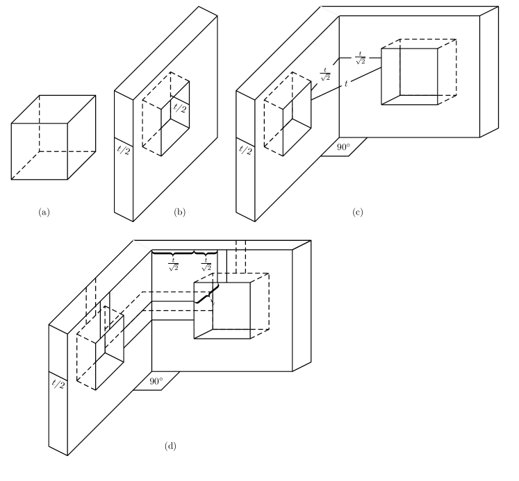
Figure 5: The dimension reducing construction. Part (a) shows the basic cubes we start with. Part (b) shows a fattened wall of width $t/2$, and its interior that gets the color 2. Part (c) shows where the minimal distance between two tiles colored 2 is attained. Part (d) presents (in full lines) the interiors of the fattened edges that get the color 3 and shows where the minimal distance between two such tiles is attained.

It is clear that the resulting 4-colored tiling can be generalized into a $(d+1)$-colored tiling of $\mathbb{R}^{d}$.

Formal definition of the construction.

For the sake of formality, we give the exact definitions of the tiles below.

For $(x,y,z)\in\mathbb{R}^{3}$, let $f(x,y,z)\in[0,a/2]^{3}$ be a motonone non-decreasing ordering of $\{\bar{x},\bar{y},\bar{z}\}$, where $\bar{b}=\min\{|b-an|:n\in\mathbb{Z}\}$. That is, we measure the minimal distance to a wall in each coordinate and arrange these minimal distances in a non-decreasing order. For example, for any $a\geq 1$, the point $(2.4a,7.8a,3.3a)$ is mapped by $f$ to $(0.2a,0.3a,0.4a)$.

• The tiles colored 1 consist of all points $(x,y,z)$ in a basic cube such that $f(x,y,z)_{1}>t/2$. (These are exactly the points that are at least $t/2$-far from each wall – the ‘interior’ of the cube.)

• The tiles colored 2 consist of points $(x,y,z)$ in a basic cube such that $f(x,y,z)_{1}\leq t/2$ and $f(x,y,z)_{2}>t/2+t/\sqrt{2}$. (These are the points that are close to a wall only in a single coordinate – the ‘interiors’ of the fattened facets.) Note that each basic cube contains six such tiles, and each such tile contains points of two adjacent basic cubes.

• The tiles colored 3 consist of points $(x,y,z)$ in a basic cube such that $f(x,y,z)_{1}\leq t/2$, $f(x,y,z)_{2}\leq t/2+t/\sqrt{2}$, and $f(x,y,z)_{3}>t/2+2t/\sqrt{2}$. (These are the points that are close to a wall in two coordinates – the ‘interiors’ of the fattened edges.) Note that each basic cube contains 12 such tiles (one for each edge), and each such tile contains points of four adjacent basic cubes.

• The tiles colored 4 consist of the rest of the points (i.e., the fattened neighborhoods of the vertices). Note that each basic cube contains 8 such tiles (one for each vertex), and each such tile contains points of eight adjacent basic cubes.

The choice of $t$.

The construction makes sure that for $i=1,2,3$, the distance between two points colored $i$ in different tiles is at least $t$. In order to guarantee the same condition for the color 4 as well, we have to choose $t$ such that the distance between two ‘neighborhoods of corners’ will be at least $t$. By the construction, this amounts to the inequality

$$a-2\left(\frac{t}{2}+\frac{2t}{\sqrt{2}}\right)\geq t,$$

or equivalently, $t\leq\frac{a}{2+2\sqrt{2}}$. Similarly, in $\mathbb{R}^{d}$ we obtain $t\leq\frac{a}{2+2(d-1)\sqrt{2}}$.

The choice of $a$.

An easy computation shows that the largest tiles are those colored 1. Hence, in order to make the volume of all tiles $\leq 1$, we have to choose $a$ such that the volume of each such tile is 1. By construction, this amounts to the equality

$$1=(a-t)^{3}=a^{3}\cdot\left(1-\frac{1}{2+2\sqrt{2}}\right)^{3},$$

or equivalently, $a=1+\frac{1}{1+2\sqrt{2}}\approx 1.261$. Similarly, in $\mathbb{R}^{d}$ we obtain $a=1+\frac{1}{1+2(d-1)\sqrt{2}}$.

The lower bound on $t$.

Summarizing the above, the value of $t$ we obtain in $\mathbb{R}^{3}$ is

$$t=\frac{a}{2+2\sqrt{2}}=\frac{1}{1+2\sqrt{2}}\approx 0.261.$$

In $\mathbb{R}^{d}$, we obtain $t=\frac{1}{1+2(d-1)\sqrt{2}}$. This gives lower bounds of $0.131$ and $\frac{1}{2+4(d-1)\sqrt{2}}$ on the fault tolerance in $\mathbb{R}^{3}$ and $\mathbb{R}^{d}$, respectively. The lower bound in $\mathbb{R}^{3}$ is superseded by the ‘bricks and balloons’ construction described below. The lower bound in $\mathbb{R}^{d}$, which is $\Omega(1/d)$, is not very far from the upper bound we obtained in Section 5.1.1 – namely, $O(\log d/\sqrt{d})$.

5.2.2 The bricks and balloons construction

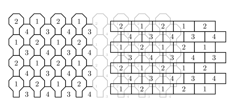
Figure 6: The bricks and balloons construction

The bricks and balloons (B&B) construction, demonstrated in Figure 6, is a periodic tiling of $\mathbb{R}^{3}$, colored in 4 colors. In order to present the tiling, we need an auxiliary notation.

Notation.

Consider the slab $D=\mathbb{R}\times\mathbb{R}\times[z_{1},z_{2}]\subset\mathbb{R}^{3}$. We say that a tiling $T_{1},T_{2},\ldots$ of $D$ is a fattened plane tiling if there exists a tiling $T^{\prime}_{1},T^{\prime}_{2},\ldots$ of the plane such that $\forall i:T_{i}=T^{\prime}_{i}\times[z_{1},z_{2}]$.

The layers of B&B.

The B&B construction is based on two fattened plane tilings:

• The brick wall layer – a fattening of a brick wall tiling of the plane. The underlying plane tiling is a periodic tiling, in which the basic unit consists of four rows of adjacent rectangles, where the even rows are indented by half a brick, making the construction look like a brick wall. In the odd rows, the colors 1,2 are used alternately, and in the even rows, the colors 3,4 are used alternately. Furthermore, the colors in the third and fourth rows are shifted by one, so that a rectangle colored $i$ is not placed right under another rectangle colored $i$, see Figure 6. The side lengths of the rectangles and the width of the slab will be specified below.

• The balloon layer – a fattening of another periodic tiling of the plane. This tiling is similar in its high-level structure to the brick wall layer, but instead of rectangles, the tiles are ‘balloons’ consisting of a regular octagon and a square built on one of its edges. The basic unit of the tiling is four columns of adjacent balloons, where the even columns are shifted in such a way that the balloons tile the plane. In the odd columns, the colors 1,2 are used alternately, and in the even columns, the colors 3,4 are used alternately. Furthermore, the colors in the third and fourth columns are shifted by one, so that a balloon colored $i$ is not placed near another balloon colored $i$ (see Figure 6). The side lengths of the balloons and the width of the slab will be specified below.

The structure of B&B.

The B&B tiling is periodic, where the basic unit consists of a brick wall layer and a balloon layer, placed one on top of the other in the way presented in Figure 6. (Note that once the two layers are placed, the coloring of one layer fully determines the coloring of the other.)

The side lengths and the slab heights.

Denote the side length of the balloon by $2a$. It is easy to see that the side lengths of the rectangles are $(2+\sqrt{2})a$ and $(4+2\sqrt{2})a$. Furthermore, the area of both a balloon and a rectangle is equal to $(12+8\sqrt{2})a^{2}$. Hence, in order to make all tiles equal-volume, we choose the height of all slabs (both in the brick wall layers and in the balloon layers) to be the same value $z$.

To find the minimal distance between two same-colored tiles, we consider several cases:

• Two same-colored balloons in the same layer: The minimal distance between two such balloons is $\sqrt{8+4\sqrt{2}}a\approx 3.696a$.

• Two same-colored bricks in the same layer: Here, the minimal distance is $(2+\sqrt{2})a$.

• A balloon and a same-colored brick at an adjacent layer: Here, the minimal distance is $a$.

• A balloon/brick and a same colored balloon/brick two layers apart: Here, the minimal distance is $z$.

Hence, the minimal distance between two same-colored tiles is $\min\{a,z\}$, and in order to optimize it we choose $z=a$.

The lower bound on $t$.

Since $z=a$, the volume of each tile is $(12+8\sqrt{2})a^{2}\cdot a=(12+8\sqrt{2})a^{3}$. Thus, in order to make the volume of all tiles equal to $1$, we fix

$$a=\left(\frac{1}{12+8\sqrt{2}}\right)^{1/3}\approx 0.350.$$

Therefore, this construction satisfies $t=a\approx 0.35$, and hence, provides a lower bound of $t/2\approx 0.175$ on the fault tolerance. This improves significantly over the fault tolerance of the dimension reducing construction (i.e., $0.131$), but is still far from the upper bound obtained in Section 5.1.1 (namely, $0.365$).

5.2.3 The close packing of boxes construction

Motivation.

This construction, a $k$-colored tiling of $\mathbb{R}^{3}$ where $k\gg 3$, is a natural generalization to $\mathbb{R}^{3}$ of the ‘honeycomb of rectangles’ construction presented in Section 4.2.2. The idea behind the construction is to choose an optimal sphere packing in $\mathbb{R}^{3}$, and construct a fattened plane tiling in which the tiles in each color are placed at the centers of the spheres of the packing. (Recall that as the number of colors is large, the size of each tile is negligible with respect to the size of its inflation, and hence, we can treat the tiles as single points.)

We use the classical HCP lattice (one of the most common closed packings, see [7]), which corresponds to a periodic sphere packing in which the basic unit is two hexagonal layers of spheres, where in the top layer, each sphere is placed on top in the hollow between three spheres in the bottom layer. The coordinates of the centers of these spheres are:

$$(r,r,r),(3r,r,r),(5r,r,r),\ldots,(2r,r+\sqrt{3}r,r),(4r,r+\sqrt{3}r,r),(6r,r+\sqrt{3}r,r),\ldots$$

for the bottom layer, and

$$(2r,r+\frac{\sqrt{3}}{3}r,r+\frac{2\sqrt{6}}{3}r),(4r,r+\frac{\sqrt{3}}{3}r,r+\frac{2\sqrt{6}}{3}r),\ldots,(r,r+\frac{4\sqrt{3}}{3}r,r+\frac{2\sqrt{6}}{3}r),(3r,r+\frac{4\sqrt{3}}{3}r,r+\frac{2\sqrt{6}}{3}r),\ldots$$

for the top layer.

The structure of the tiling.

Assume that the number of colors is $k=m^{3}$. Each tile is a box with side lengths $(a,b,c)$ to be determined below, and the basic unit is a ‘large box’, which is an $m\times m\times m$ cubic block of tiles, using all the $k=m^{3}$ colors (in arbitrary order). Then, the basic unit of the construction is a two-layer fattened plane tiling, in which each layer is a fattened copy of the ‘honeycomb of rectangles’ tiling. The upper layer is shifted by $\frac{m}{2}a$ in the $x$-coordinate and by $\frac{\sqrt{3}m}{6}a$ in the $y$-coordinate, so that the corners of the large boxes lie in the coordinates of the sphere centers described above (for $r=\frac{m}{2}a$). A quick calculation shows that in order to make this possible, the proportion $(a:b:c)$ should be approximately $(2:\sqrt{3}:2\sqrt{6}/3)$ (where we neglect the size of each tile with respect to the size of the inflation, which can be absorbed in an $1+o(1)$ multiplicative factor in the final value of $t$). The volume of each tile is clearly $abc$. In order to make the volumes of all tiles equal to $1$, we need

$$a\cdot\frac{\sqrt{3}}{2}a\cdot\frac{\sqrt{6}}{3}a=1,$$

and thus, $a=(6/\sqrt{18})^{1/3}=2^{1/6}\approx 1.122$. Hence, the side lengths of each tile are

$$(2^{1/6},3^{1/2}/2^{5/6},2^{2/3}/3^{1/2})\approx(1.122,0.972,0.916),$$

and the minimal distance between two same-colored points in different tiles is

$$(m-1)a=(2^{1/6}+o(1))k^{1/d},$$

which matches the upper bound proved in Section 5.1.1.

Generalization to higher dimensions.

A similar tiling can be constructed to match any lattice sphere packing, assuming the number of colors $k$ is sufficiently large with respect to $d$. Hence, any dense lattice sphere packing can be translated into a lower bound on the asymptotic fault tolerance of rounding schemes in the corresponding dimension. In particular, as the E8 lattice and the Leech lattice which attain the maximal possible density of sphere packings in dimension 8 and 24 (respectively) are lattice packings, they can be translated to box tilings showing that the asymptotic upper bounds on the fault tolerance in $\mathbb{R}^{8}$ and $\mathbb{R}^{24}$ proved in Section 5.1.1 are tight.

6 Summary

In this paper we demonstrated that the natural problem of how to round points in $\mathbb{R}^{d}$ with optimal fault tolerance using a tiny amount of side information is tied to deep problems on space partitions and sphere packings. We proposed a new way to look at the problem as colored tilings of the space, and related it to a generalized type of error correcting code in which we inflate tiles into Minkowski sums rather than points into balls. We obtained a number of tight asymptotic bounds for a large number of colors, as well as lower and upper bounds for small numbers of colors, but finding the optimal solutions for particular numbers of colors and dimensions is still wide open.

References

- [1] E. Alkim, L. Ducas, T. Pöppelmann, and P. Schwabe, Post-quantum key exchange – A new hope, proceedings of USENIX 2016, pp. 327–343.
- [2] M. L. Balinsky, How should data be rounded?, Lecture Notes - Monograph Series, Vol. 28: Distributions with Fixed Marginals and Related Topics, Institute of Mathematical Statistics, 1996, pp. 33-44.
- [3] H. Busemann, Convex surfaces, Interscience Publishers, New York, 1958.
- [4] R. Bott and L.W. Tu, Differential Forms in Algebraic Topology, Springer, New York, 1982.
- [5] H. Cohn, A. Kumar, S. D. Miller, D. Radchenko, and M. Viazovska, The sphere packing problem in dimension 24, Ann. of Math. 185(3) (2017), pp. 1017–1033.
- [6] J. H. Conway and N. J. A. Sloane, What are all the best sphere packings in low dimensions?, Discrete Comput. Geom. (László Fejes Tóth Festschrift), 13 (1995), pp. 383-–403.
- [7] J. H. Conway and N. J. A. Sloane, Sphere packing, lattices and groups (3rd edition), Springer-Verlag, New York, 2013.
- [8] L. H. Cox and L. Ernst, Controlled rounding, Information Systems and Operational Research, 20(4) (1982), pp. 423–432.
- [9] M. de Berg, O. Cheong, M. van Kreveld, and M. Overmars, Computational Geometry (3rd ed.), Springer-Verlag, 2008, pp. 121–-146.
- [10] Y. Dodis, R. Ostrovsky, L. Reyzin, and A. D. Smith, Fuzzy extractors: How to generate strong keys from biometrics and other noisy data, SIAM J. Comput. 38(1) (2008), pp. 97–139.
- [11] L. Fejes-Tóth, Some packing and covering theorems, Acta Sci. Math. Szeged, 12 (1950), pp. 62–67.
- [12] B. Fuller, L. Reyzin, and A. Smith, When are Fuzzy Extractors Possible?, IEEE Trans. Inform. Theory, to appear.
- [13] T. C. Hales, A proof of the Kepler conjecture, Ann. of Math. 162 (2005), pp. 1065-–1185.
- [14] P. Indyk, R. Motwani, P. Raghavan, and S. S. Vempala, Locality-preserving hashing in multidimensional spaces, proceedings of STOC 1997, pp. 618–625.
- [15] A. Juels and M. Wattenberg, A fuzzy commitment scheme, proceedings of ACM CCS 1999, pp. 28–36.
- [16] G. Kindler, R. O’Donnell, A. Rao, and A. Wigderson, Spherical cubes and rounding in high dimensions, proceedings of FOCS 2008, pp. 189-198.
- [17] G. Kindler, A. Rao, R. O’Donnell, and A. Wigderson, Spherical cubes: optimal foams from computational hardness amplification, Commun. ACM 55(10) (2012), pp. 90–97.
- [18] J. Snoeyink, Point location, in: J. E. Goodman, J. O’Rourke, and C. D. Tóth (eds.), Handbook of Discrete and Computational Geometry, 3rd edition, CRC Press, Boca Raton, FL, 2017.
- [19] M. Viazovska, The sphere packing problem in dimension 8, Ann. of Math. 185(3) (2017), pp. 991–1015.
- [20] L. Willenborg and T. de Waal, Elements of statistical disclosure control, Lecture Notes in Statistics 155, Springer, 2001.
- [21] G. M. Ziegler, Lectures on Polytopes, Graduate Texts in Mathematics, 152, Springer-Verlag, 1995.