Using social media to measure demographic responses to natural disaster: Insights from a large-scale Facebook survey following the 2019 Australia Bushfires

Abstract

In this paper we explore a novel method for collecting survey data following a natural disaster and then combine this data with device-derived mobility information to explore demographic outcomes. Using social media as a survey platform for measuring demographic outcomes, especially those that are challenging or expensive to field for, is increasingly of interest to the demographic community. Recent work by Schneider and Harknett (2019) explores the use of Facebook targeted advertisements to collect data on low-income shift workers in the United States. Other work has addressed immigrant assimilation (Stewart et al, 2019), world fertility (Ribeiro et al, 2020), and world migration stocks (Zagheni et al, 2017). We build on this work by introducing a rapid-response survey of post-disaster demographic and economic outcomes fielded through the Facebook app itself. We use these survey responses to augment app-derived mobility data that comprises Facebook Displacement Maps to assess the validity of and drivers underlying those observed behavioral trends. This survey was deployed following the 2019 Australia bushfires to better understand how these events displaced residents. In doing so we are able to test a number of key hypotheses around displacement and demographics. In particular, we uncover several gender differences in key areas, including in displacement decision-making and timing, and in access to protective equipment such as smoke masks. We conclude with a brief discussion of research and policy implications.

1 Introduction

Demographers have long been interested in large-scale natural disasters and their effects on regional populations (Frankenberg et al, 2014). This topic has only increased in importance as climate change and rising population densities increased the observed frequency of natural disasters which impact human settlements (Bouwer, 2011).

Researchers have used mobility data from cell phones and other electronic devices to characterize both short-term and long-term displacement after a disaster (Gething and Tatem, 2011); however, this technique has often been limited by an inability to pair mobility data with key additional information. In particular, many potential hypotheses could be explored if these methods also gave information about who is displaced, the household structure of displaced persons, and the nature of locations to which displaced persons migrate (e.g. identification as a home of relatives) (Frankenberg et al, 2014).

Migration decisions are complex and depend on not only the severity of a given disaster, but also the demographic composition of those in the area (Frankenberg et al, 2014). A displacement event can last anywhere from days to years, with many choosing to permanently relocate. Prior work has compared mobility strategies among individuals living in communities which sustained different degrees of damage due to the 2004 Indian Ocean Tsunami (Frankenberg et al, 2014). Drawing from a recent example of a severe disaster, we observe that in 2010 Port-au-Prince, Haiti lost 23% of its permanent residents following a magnitude 7.0 earthquake struck near that city (Frankenberg et al, 2014). Understanding demographic heterogeneity among affected populations can help us better understand these disparities, and can better inform policy response to such events in the future.

Prior large-scale post-disaster surveys are discussed in the literature, but these studies are expensive to conduct and rare precisely due to the difficulty of reaching displaced populations (Frankenberg et al, 2014). One recent attempt utilized surveys conducted on the Facebook ad system in 2018 following the Hurricane Maria disaster in Puerto Rico (Alexander et al, 2019). We extend this work by surveying directly on the Facebook platform rather than through advertisements, which gives us finer control over sampling, more ability to perform bias correction, and further lowers the cost of this work.

In this study we partner with Facebook’s Data for Good program to address the above limitations of post-disaster displacement surveys. The Data for Good program has already used mobility data to develop an approach that both identifies migration and relocation after disasters (Maas et al, 2019) and provides real-time information about displacement to non-governmental organizations (NGOs). In this study we extend their work by incorporating additional demographic and contextual information collected via a rapid-deployment survey following a disaster. Rapid surveys on a platform such as Facebook provide a novel way of reaching individuals in situations that would otherwise render them prohibitively expensive or impractical to reach, and allow for high-quality demographic estimates in otherwise adverse circumstances.

From September 2019 to March 2020, Australia experienced one of the worst bushfires in modern history (Kganyago and Shikwambana, 2020). Over this period it is estimated that 186,000 square kilometres were burned and 5,900 building were destroyed. This included more than three thousand homes (Filkov et al, 2020) and resulted in the displacement of tens of thousands of Australians. To better understand the economic and demographic effects of this disaster in Australia, we conducted a survey of Facebook users who could have been directly affected by the bushfires. This, when combined with mobility estimates provided by the Data for Good program, allows us to refine estimates derived from mobility data (Maas et al, 2019) and to address hypotheses around how displacement affected people and households in the region – information that cannot be obtained from observational migration data alone.

This research provides two major contributions to the literature on demography and disasters: (1) we demonstrate the viability of using a rapid-deployment on-platform Facebook survey to collect demographic data following a natural disaster; and (2) we characterize the demographics displaced persons following 2019 Australia bushfires. Specifically, this survey allowed us to characterize the impact of displacement from the Australia bushfires on a representative sample of Australian Facebook users and test key hypotheses in short term migration around disaster-induced displacement. To these ends, we surveyed 95,649 Facebook users who were over the age of 18 and predicted to be in the area affected by two major bushfires: the Green Wattle Creek Fire in Eastern New South Wales and the Cudlee Creek Fire in Adelaide Hills, South Australia. Both of these fires started on or about December 18, 2019.

This article is laid out in the following manner: (1) Literature review; (2) Research hypotheses; (3) Data and methods; (4) Survey descriptive statistics; (5) Analysis; and finally (6) Discussion and limitations.

2 Literature Review

Demographers have studied the population consequences of disasters for a number of specific outcomes. Typically these include issues such as fertility (Lin, 2010), mortality (Finlay, 2009) and migration (Belasen and Polachek, 2013; Frankenberg et al, 2014). This work primarily focuses on understanding the latter with an emphasis on demographics of age, gender and household mobility. We build on the rich literature on the sociology of disasters (Dynes et al, 1987) with an emphasis on demography and disasters. Here, we employ Kreps’s definition of “disaster” as used in Smelser et al (2001), which defines disasters as “non-routine events in societies that involve conjunctions of physical conditions with social definitions of human harm and social disruption.”

This section is laid out as follows, first we review the literature on migration and disasters, then we cover the basics of Facebook’s Data for Good Displacement map; next, we review briefly the automated displacement measurements compiled from cellular phone data and apps, and finally we review the literature of surveys being conducted on Facebook for demographic estimates and detailed information and generalizability to offline populations.

2.1 Disasters and Demography

The literature on the demography of disasters can be laid-out in five core themes: (1) fertility, (2) mortality, (3) health, (3) migration and (4) data collection (Frankenberg et al, 2013). This topic is important, having warranted a special issue in Population and Environment (Frey and Singer, 2010; Gutmann and Field, 2010; Stringfield, 2010; Hori and Schafer, 2010; Davies and Hemmeter, 2010; Czajkowski and Kennedy, 2010; Plyer et al, 2010), which focused on the demographic impacts of Hurricane Katrina in the United States.

Disasters, in general, have the potential to displace people through either preemptive effects (e.g. early evacuation) or direct damage property and economic livelihood. Both voluntary and involuntary displacement can effect demographic change in a local area (Frankenberg et al, 2014). These demographic changes can have material consequences for affected areas (Frankenberg et al, 2013). For example, Fussell et al (2010) shows that Hurricane Katrina affected the racial and ethnic composition of New Orleans through disproportionate housing damage experienced by Black residents. Another example, which used a large-scale survey, includes Gray et al (2014) which compared mobility strategies among individuals living in small villages. Smith and McCarty (1996) studied the effects of Hurricane Andrew. This disaster resulted in the displacement of more than 350,000 individuals, around 40,000 of which were estimated to have never returned. Other significant studies in the migration of people due to disasters includes Raker (2020); Schultz and Elliott (2013); James and Paton (2015); and Donner and Rodríguez (2008).

2.2 Facebook’s Gender-Stratified Displacement Map

Facebook’s Data for Good program is a broad initiative designed to provide data to humanitarian organizations to facilitate their important work in many fields, including disaster response and disease prevention. One such dataset is the Gender-Stratified Displacement Map, which aims to quantify the magnitude of displacement following disasters and describe where the displaced population has migrated, and enables study of these population trends by gender. As climate change increases the frequency and severity of natural disasters, it becomes more important for response organizations to utilize novel data sources in understanding how many people are displaced, where they have been displaced, and when they might be able to return home. Facebook is uniquely positioned to aid organizations in answering these questions, helping increase the effectiveness of humanitarian response of food, medical and housing aid while preserving user privacy.

Briefly, Facebook’s Displacement Map dataset estimates how many people were displaced by a given disaster and where those people are in the period following it at an aggregate level. Specifically, the models identify a person as displaced if their typical nighttime location patterns are disrupted after the event compared to that person’s pre-disaster patterns. These patterns are obtained from a user’s Location History, which is an optional setting on the Facebook app users can enable that provides precise locations . The individual data is aggregated into a city-level transition matrix showing how many people are displaced from one city to another for all source cities in the disaster affected region for each day for a period following the event . These aggregate trends, stratified by gender, have revealed gender differences in the patterns of displacement and return that we seek to investigate further through the lens of this survey. We articulate specific hypotheses generated by these observed displacement trends below in Section 4.

2.2.1 Other Methods for Automatically Measuring Displaced Populations

There is a growing literature around using cell-phone and app-based data for research around location and migration, which includes short-term displacement due to disasters. For example, Lu et al (2012) involved the use of 1.9 million phone users’ location data subsequent to and for up to one year after the 2010 Haitian earthquake. This work was able to uncover very detailed mobility patterns among the studied population. Deville et al (2014) follows up on this work and demonstrates the cost effectiveness of using mobile phone network data for accurate and detailed maps of populations after a disaster. This is an active area of the literature, which is also being used to estimate the population of countries that have historically had weak or non-existent demographic data (Tatem, 2017).

2.3 Facebook for Demographic Surveys

There is much work looking into the viability of using Facebook as survey platform for demographic data. Schneider and Harknett (2019) explore the use of Facebook targeted advertisements to collect data on low-income shift workers in the United States. Blondel et al (2015) uses Facebook ads system to recruit survey participants to answer issues of mobility and geographic partitioning. Alexander et al (2019) has employed Facebook ads system to survey out-migration following a hurricane in Puerto Rico in 2017. Surveys administered via Facebook ads system has also been used to measure immigrant assimilation (Stewart et al, 2019), world fertility (Ribeiro et al, 2020), and world migration stocks (Zagheni et al, 2017). There is a growing literature on how to re-adjust surveys administered on Facebook ads (Zagheni et al, 2017) platform or survey system (Feehan and Cobb, 2019) for estimation of both online and offline populations.

3 Australia Bushfires, 2019-2020

The most recent census data for Australia places the country’s total population at around 26 million, (2016) and estimates of the economic impact of bushfires ranging from 1.8 billion to 4.4 billion (AUD). In this work we focus on the Green Wattle Creek Fire in Eastern New South Wales and the Cudlee Creek Fire in Adelaide Hills, South Australia (Figure 1), both of which started on or about December 18th, 2020. The Green Wattle Creek fire was extinguished by rainfall in February 2020 and is estimated to have destroyed 467,000 acres of land. The Cudlee Creek Fire was put out by Australian firefighters and damage was estimated at 57,000 acres .

4 Research hypotheses

Data limitations have long hampered the study of policy and population responses to natural disasters. The Facebook survey employed in this study allows us to address decision-making and policy-focused questions around disaster displacement. In this work we focus on five important hypotheses around displacement, gender and age.

In this survey we asked about duration of displacement (operationalized as 3 categories: not displaced, displaced 1 to 3 nights, and displaced more than 3 nights). While there is some research characterizing populations displaced by disasters, this research either leverages on-the-ground survey modes (e.g. Frankenberg et al (2014)), which are both expensive and difficult to execute in affected regions, or leverage data provided by cell phones and other tracking apps. The latter lacks identifying demographic information and limits insights into why people left a given disaster area. This work provides two significant advances in researching demographic responses to disasters: (1) it demonstrates the cost effectiveness and ease of implementation of an in-app survey following a disaster and (2) it allows us to ask demographic, migration and economic questions to hypotheses that are rarely tested in the disaster and demography literature Frankenberg et al (2014). Below are a series of hypotheses we explored.

Our research hypotheses focused on six key themes related to demographic and policy decision making for disaster relief. First we focused on who evacuates and how; second we looked into who made decisions to evacuate; third we tested where people went when they evacuated; fourth we looked into what circumstances households became separated during displacement; fifth, we explored job disruption due to the disaster; and finally we tested for inequalities in access to and knowledge of protective equipment (masks) during a disaster.

Question 1

Who evacuates and how?

Null Hypothesis 1

There will not be differences in who evacuates or how they evacuate by demographic characteristics.

Alternative 1

There will be differences in who evacuates, when they evacuate, or how they evacuate by demographic characteristics. Based on trends in Facebook’s Displacement Maps, we have reason to believe that women will evacuate differently, on average, than men. We will assess whether survey responses are consistent with these behavioral signals.

Survey Questions

We test this hypothesis with questions on evacuation timing and displacement duration, as well as distance of displacement relative to home, in conjunction with questions measuring demographic characteristics.

Question 2

Who makes the decision to evacuate?

Null Hypothesis 2

There will be no differences in attribution of the evacuation decision by demographic characteristics.

Alternative 2

There will be differences in attribution of the evacuation decision by demographic characteristics. For example, men will be more likely to take ownership of the decision for their household to evacuate.

Survey Questions

We test this hypothesis with a question on who made the decision to evacuate.

Question 3

Where do people go when they evacuate?

Null Hypothesis 3

People will evacuate primarily to nearby towns and areas which are not affected by the disaster.

Alternative 3a

People will relocate equally to nearby and distant locations from the disaster.

Alternative 3b

People will relocate primarily to locations far from the disaster.

Survey Questions

Among people who evacuated, we ask respondents where they evacuated relative to their home (e.g. same city).

Question 4

Under what circumstances do households separate during displacement?

Null Hypothesis 4

Household separations will not meaningfully depend on demographic characteristics.

Alternative 4

Household separations will meaningfully depend on demographic characteristics. For example, women may evacuate earlier than the rest of their household and men may return from displacement before the rest of their household.

Survey Questions

We asked about household separation upon leaving the disaster area and also when returning to home.

Question 5

Whose work is disrupted?

Null Hypothesis 5

Work disruption will not meaningfully depend on demographic characteristics after controlling for economic situation.

Alternative 5

Work disruption will meaningfully depend on demographic characteristics after controlling for economic situation. For example, women may be more impacted by work disruption.

Survey Questions

We ask the respondent if their work was disrupted due to the bushfires.

Question 6

Who has access to masks and the knowledge to use them effectively?

Null Hypothesis 6

An individual’s knowledge of or access to masks during a bushfire will not depend meaningfully on demographics.

Alternative 6

An individual’s knowledge of or access to masks during a bushfire will depend meaningfully on demographics. For example Thomas et al (2015) found that in the United States men had odds ratio of 2.5 times the knowledge and access to key equipment for disaster response.

Survey Questions

We ask about access and knowledge of using an N95 mask.

Summary

We will explore each of these hypotheses with the survey data (See Appendix for full descriptive statistics). In this work we will employ inferential statistics and regression analysis to fully review each hypotheses and question set.

5 Data and Methods

5.1 Survey Population

We surveyed an effectively random sample of 95,649 Facebook users over the age of 18. Each of these users answered an array of questions on demographics, smoke masks, and whether they were in the region at the time of the fires. Of those surveyed, 24,486 Facebook users were in the area of the two major bushfires under consideration in this article. Here, we are focusing on two bushfires that started on or about December 18, 2019 – the Green Wattle Creek Fire in Eastern New South Wales and the Cudlee Creek Fire in Adelaide Hills, South Australia (Figure 1). Of those who said they were in the area, 7,073 users said they were affected by the fires (Q 2: loc_q). These users were then asked a detailed set of questions on displacement outcomes. To guarantee we only consider the target population, we limit our displacement-related analysis to these 7,073 users. This is, effectively, a form of rejection sampling and will maintain our sample properties (Gilks and Wild, 1992). The survey was in the field for two weeks, from February 20, 2020 to March 5, 2020, approximately two months after the bushfires began. This timing strikes a balance between decaying respondent recall and allowing the consequences of a displacement to play out more fully.

5.2 Sample Design

The sampling design is built to capture a representative sample of Facebook users who were 18 or older and predicted to be in the disaster region of the Green Wattle Creek and Cudlee Creek fires (Figure 1). Through a combination of app-based user targeting (e.g. in Australia) and survey gatekeeping (e.g. Q2) we are able to isolate these respondents. Specifically, we take all Facebook users who have been identified to be in the region based on their city location and age. We also include users as identified by their Location History as reported in Facebook’s Data for Good program Displacement Map. We are then able employ rejection sampling to limit our final respondent set to only included the target population. This method is very general and will provide a random sample of users in the two regions (Gilks and Wild, 1992). We are able to adjust for survey non-response through the application of survey weights (see Section 5.3). All users were asked for informed consent to survey and all questions allowed the respondent to not respond (See Question 1). No participants were compensated in any way for their participation.

Though we are able to predict with some accuracy whether a respondent was in the area of a bushfire, we still take steps in the survey to validate this. All respondents must self-identify in the survey as having been in the area of one of the two bushfires under study in December, 2019. Again, though we are able to predict with some accuracy the length of displacement for a number of our respondents, we verify in the survey whether they were displaced and for how long. An example survey question can be seen in Figure 2.

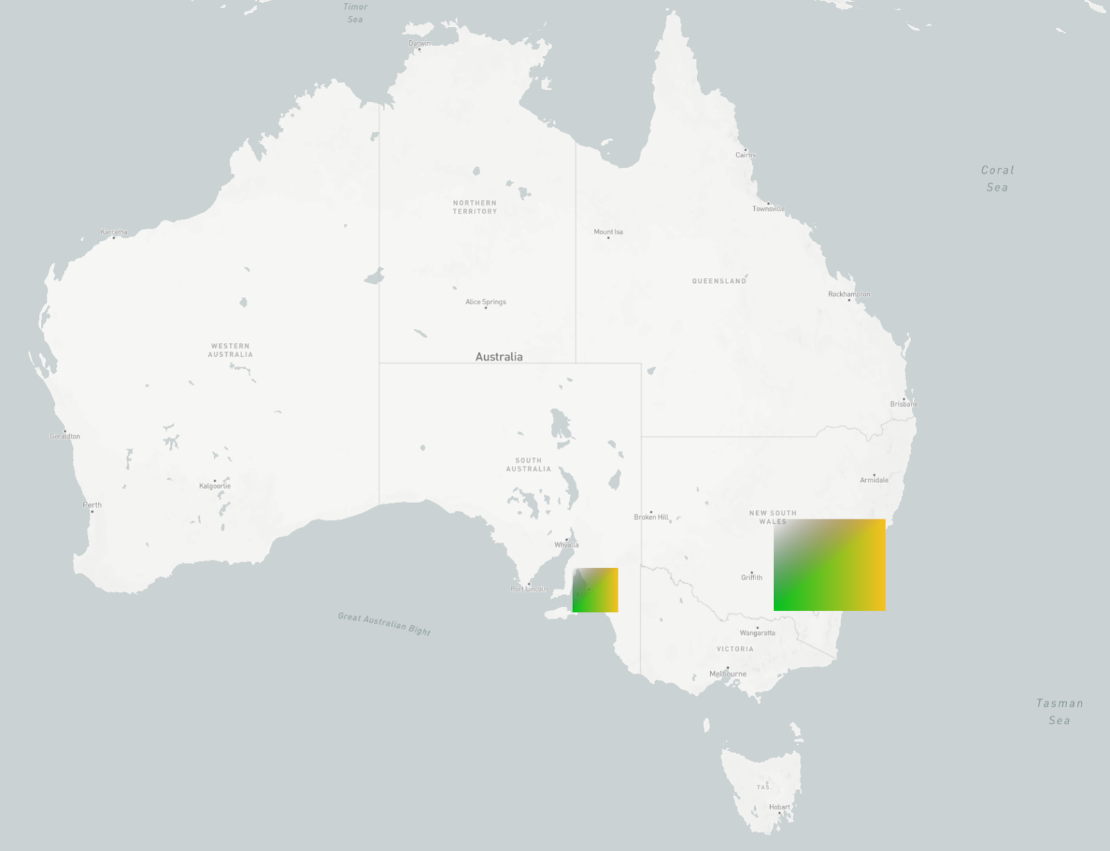
Figure 1: Map of the bounding box survey locations: Green Wattle Creek Fire in Eastern New South Wales and the Cudlee Creek Fire in Adelaide Hills South Australia.

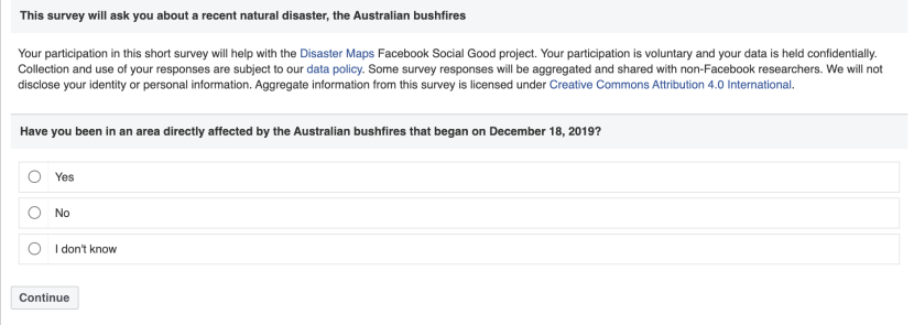
Figure 2: Example survey question from the Facebook Australia Bushfire survey.

5.3 Sample Weights for Non-Response Bias

We employ calibration (e.g raking) weights to adjust the sample to be representative of the over 18 Facebook population for the two regions under study. To do this we weight on age, gender, engagement (number of days active in a month), region, and if the user has location history turned on. This improves the representativeness of our results among both core demographics and other key Facebook user categories. All statistics discussed in this article are re-weighted and employ Horvitz-Thompson estimator for computing the weighted mean with standard errors computed using the delta method (Overton and Stehman, 1995).

6 Survey Descriptive Statistics

In Table LABEL:demographics we provide respondent counts and basic demographic summary statistics. Further, based on the Australian demographics from 2016 (most recently available data) we have added the most recent census population proportions for comparison. Our sample is more female than expected by about 3%. Age skews young with more people in the 20-39 age group than we expect by population and few in 40-70+. We have a more educated population with 31.9% bachelors degree holders or higher compared to 22% in the general population (not in table because the Australian census breaks down education differently than in our survey). For income our sample contained 18.9% of people with less than $3,200 (Australian dollars) total household monthly income compared to an expectation of around 20%. The single household distribution (household size of 1) is slightly less than expected at 12.3% compared to 15.8% in the broader population. Overall we collected sufficient information to allow for proper controlling for age and gender in our analysis despite these sample biases. For descriptive statistics we adjust using the weights discussed in Section 5.3.

Table 1: Distribution of Sample Demographics

				Australia Census
Demographic	Response	N	Percent in Sample	Pop. Percentiles
Reported Gender
	Female	42230	54.2 (53.6, 54.7)	50.7
	Male	35717	45.8 (45.3, 46.4)	49.3
Reported Age
	$<$20	6171	7.7 ( 7.4, 8.1)	6.0
	20-29	17984	22.6 (22.2, 23.0)	13.4
	30-39	16200	20.3 (19.9, 20.8)	15.0
	40-49	12971	16.3 (15.9, 16.7)	13.6
	50-59	10692	13.4 (13.0, 13.8)	12.7
	60-69	7785	9.8 ( 9.4, 10.1)	10.7
	70+	4643	5.8 ( 5.5, 6.1)	10.7
	Prefer Not to Say	3200	4.0 ( 3.8, 4.3)
Education
	Elementary	663	2.0 ( 1.7, 2.4)
	Junior High	1291	4.0 ( 3.6, 4.4)
	High School	9417	29.1 (28.3, 29.9)
	Community College	6996	21.6 (20.9, 22.3)
	University	5554	17.2 (16.5, 17.8)
	Graduate School	4750	14.7 (14.1, 15.3)
	Prefer Not to Say	3711	11.5 (10.9, 12.1)
Employment Type
	Managing a Business	5506	8.0 ( 7.7, 8.3)
	Employed by Business	25350	36.8 (36.2, 37.3)
	Employed, not by Business	2686	3.9 ( 3.7, 4.1)
	Government Work	5983	8.7 ( 8.4, 9.0)
	Student	5329	7.7 ( 7.4, 8.1)
	Retired	7898	11.5 (11.0, 11.9)
	Not Working	7689	11.2 (10.7, 11.6)
	Prefer Not to Say	8484	12.3 (11.9, 12.7)
Income
	$<$ $3,200	5892	18.9 (18.1, 19.7)
	$3,200-$5,800	4263	13.7 (13.1, 14.3)
	$5,800-$9,100	2877	9.2 ( 8.8, 9.7)
	$9,100-$14,000	1547	5.0 ( 4.6, 5.3)
	$>$ $14,000	1624	5.2 ( 4.8, 5.6)
	Prefer Not to Say	14918	47.9 (47.0, 48.8)
Household Head
	Yes	24727	34.9 (34.3, 35.4)
	No	31150	43.9 (43.3, 44.5)
	Prefer not to say	15062	21.2 (20.7, 21.7)
Household Size
	1	8964	12.3 (11.8, 12.7)	15.8
	2	20319	27.8 (27.3, 28.3)
	3	14392	19.7 (19.2, 20.1)
	4	14910	20.4 (19.9, 20.8)
	5	8197	11.2 (10.8, 11.6)
	6 or more	6360	8.7 ( 8.4, 9.0)
Household Child Count
	0	42914	58.7 (58.1, 59.2)
	1	12010	16.4 (16.0, 16.8)
	2	10701	14.6 (14.2, 15.0)
	3	4424	6.0 ( 5.8, 6.3)
	4	1653	2.3 ( 2.1, 2.4)
	5 or more	1453	2.0 ( 1.8, 2.2)
Household Partner
	Yes	37940	53.2 (52.6, 53.8)
	No	26162	36.7 (36.1, 37.3)
	Prefer not to say	7163	10.1 ( 9.7, 10.4)

7 Results and Analysis

7.1 Results on Evacuation and Return

7.1.1 Who evacuates and how?

Among people in the affected areas, 25.5%, or about 1,500, of our respondents report being displaced more than one night, with no difference in the rate by gender. However, in a regression model adjusted for age, gender, categorical groups for income, and head of household, we see that lower incomes were associated with higher odds of reporting displacement (Figure 3).

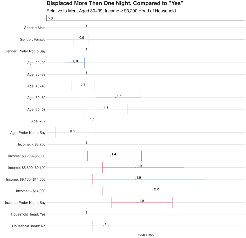
Figure 3: Odds ratios for not being displaced for more than one night, as compared to ”Yes” displaced more than one night, adjusted for age, gender, income, and head of household. People less likely to be displaced include higher income groups, people 50-59, and not head of household. Values presented in Appendix Table LABEL:Total_weights_q11_one_night_regression_no_interaction_with_income.

Of those displaced more than one night, 63.4% report displacement of more than three nights. This suggests a substantial disruption to most people’s lives caused by their displacement, with implications for policy response. For example, knowing that such a high share of respondents experienced longer displacements would suggest remedies and mitigations focusing on housing and including food and water access.

In Australia, people did not report taking advantage of government-provided transportation, though we do have difficulty assessing the availability of such assistance. Of those displaced, only 5.5% of people reported using government-provided transportation. In fact, the vast majority of people who evacuated report leaving by car, at 89%. That private transit was a key tool for evacuation again has clear policy response implications for future disasters.

7.1.2 Who makes the decision to evacuate?

Asked “Whose decision first led to you leaving your home?,” the plurality responded that it was their own decision (47.7%), while 24.3% and 23.6% attributed the decision to a family member or the government, respectively. Men were significantly more likely to say it was their own decision, while women were more likely to say it was a government decision (Figure 4).

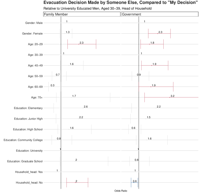
Figure 17: Evacuation decision made by someone else, compared to “my decision”; relative to university educated men, aged 30-39, head of household based on model with main effects for age, gender, education, and head of household with no interactions. Values presented in Appendix Table LABEL:Total_weights_q29_evacuation_decision_regression_no_interaction.

This result held up in regression models adjusted for gender, age, and education as collected through the survey instrument, and whether the person was the head of their household, with an odds ratio of 2.3 for women reporting government as compared to their own decision (Appendix Figure 17, Appendix Table LABEL:Total_weights_q29_evacuation_decision_regression_no_interaction). In these models, people who were not head of household had twice the odds of attributing the evacuation decision to a family member. We should note that these results reflect what people report to us; it’s entirely possible that the same sequence of events - say the government advises a person to evacuate and they do - can result in different attributions for the decision, depending on whether the person views following the advice as ultimately their own decision, or as stemming from the government’s decision. These biases are, however, known to the survey literature and the survey is designed to minimize this to the extent possible.

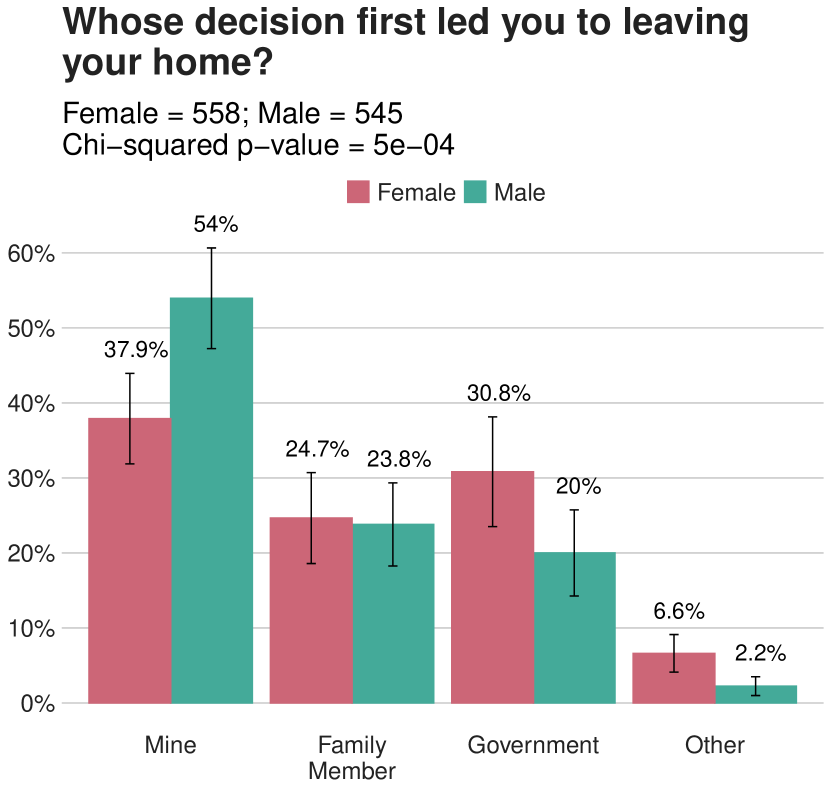
Figure 4: Men are significantly more likely to say that the decision to evacuate was their own, while women are more likely to attribute it to the government.

7.1.3 Where do people go when they evacuate?

Of people who evacuated, the majority (63.4%) evacuated to a different city in their region, with a much smaller fraction going somewhere else in their same city (30%) or to a different state in Australia (5.4%). In our survey data, women were significantly more likely to report that they evacuated within their home city (Figure 5). This is particularly interesting, as we see this consistently reflected in the behavioral data we have from aggregate trends in Displacement maps for numerous disasters around the world.

Figure 5: Women are more likely to evacuate within the same city as their home. This corresponds with trends in the Displacement Map data across many disasters and geographies.

7.1.4 Under what circumstances do households split up during displacement?

To understand the extent to which households were splitting up during displacement, we asked two questions:

• When you were displaced for more than three nights did anyone in your household stay behind?

• Did you return home at least one day before other members of your household?

Overall, we found that a substantial portion of households do split up either at the beginning (28%) or end (31.2%) of their displacement. Surprisingly, the responses to these two questions are uncorrelated, which is to say that people with a household split during departure are no more likely to split up on return, compared to households that did not split when leaving.

The vast majority of displaced people (86%) had returned home by the time we surveyed two months after the fires. Among displaced people, 42% were displaced for less than seven days, 33% for 7 to 14 days, 13% for 14 to 30 days, and 9% longer than a month. Those who had not returned home cited a range of reasons including: unsafe (57.5%), new opportunities (22.2%), being unable or unwilling (9.7%), or not allowed (8%).

While we did not see gender differences for households splitting upon departure, we found that men return home sooner than their household more frequently than women do (Figure 6). This is also consistent with the behavioral data we have for Displacement Maps outputs in many countries, including Australia.

Figure 6: Men are significantly more likely to return home ahead of the other members of their household. This is consistent with behavior trends observed in the Displacement Map.

In a regression model adjusted for age, gender, education, head of household, and any children in the household: men (OR = 2.1), people aged 50-59 (OR = 2), heads of household (OR = 2.4) and people with any children (OR = 1.6) are the groups more likely to return home ahead of their households (Figure 7). People without a university degree are significantly less likely to return home ahead.

Figure 7: Odds ratio for returning home ahead of the rest of the household, as compared to not, adjusted for age, gender, education, household head, and any children. Values presented in Appendix Table LABEL:Total_weights_q26_household_split_return_no_ref_regression_no_interaction_with_child_count_reformulated.

7.1.5 Whose work is disrupted?

Among displaced people asked: “Did leaving your home prevent you from working as much as you normally do?”, 54.7% of people said “yes.” These responses did not significantly differ by gender. It is perhaps unsurprising that in a model adjusted for age, gender, and education, people who were displaced for more than three nights were significantly more likely (OR = 1.8) to report that they were prevented from working, as compared to people displaced fewer nights (Appendix Table LABEL:Total_weights_q21_prevent_working_regression_no_interaction_with_income_displacement_reformulated). Nonetheless, this underscores the importance of duration of displacement on the degree of disruption in people’s lives.

7.2 Gender Differences in Mask Access and Knowledge

7.2.1 Mask Access

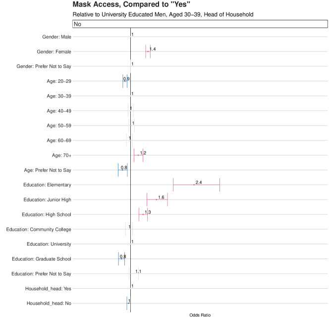
Figure 18: Mask access, compared to “yes”; relative to university educated men, aged 30-39, head of household based on model with main effects for age, gender, education, and head of household with no interactions. Values presented in Appendix Table LABEL:Total_weights_q28_mask_access_regression_no_interaction.

When asked “Do you have access to a face mask in case of excessive wildfire smoke?” 38% of the more than 61,000 people who responded said “Yes.” However, there were significant gender differences (Figure 88(a)). Men were significantly more likely to report mask access. In a regression model adjusted for age, gender, education, and head of household, women were significantly more likely (OR = 1.4) to say that they did not have mask access (Appendix Figure 18, Table LABEL:Total_weights_q28_mask_access_regression_no_interaction).

(a) Mask Access by Gender

(b) Mask Knowledge by Gender

Figure 8: Men are significantly more likely to report that they had access to N95 smoke masks during the Australian bushfires in December 2019, and that they can tell if a mask is effective.

7.2.2 Mask Knowledge

In addition to less mask access, women were also significantly more likely (OR = 1.6) to report that they do not know how to tell if a face mask is effective against wildfire smoke, compared to men (Figures 88(b), 9). This is after already adjusting for the difference in mask access, in addition to age, education, and head of household.

In the model, people without mask access had five times the odds of not knowing whether a mask was effective (OR = 5.4), compared to people who did (Figure 9). People who reported that they were not the head of household were also significantly more likely (OR = 1.2) to not know whether a mask was effective.

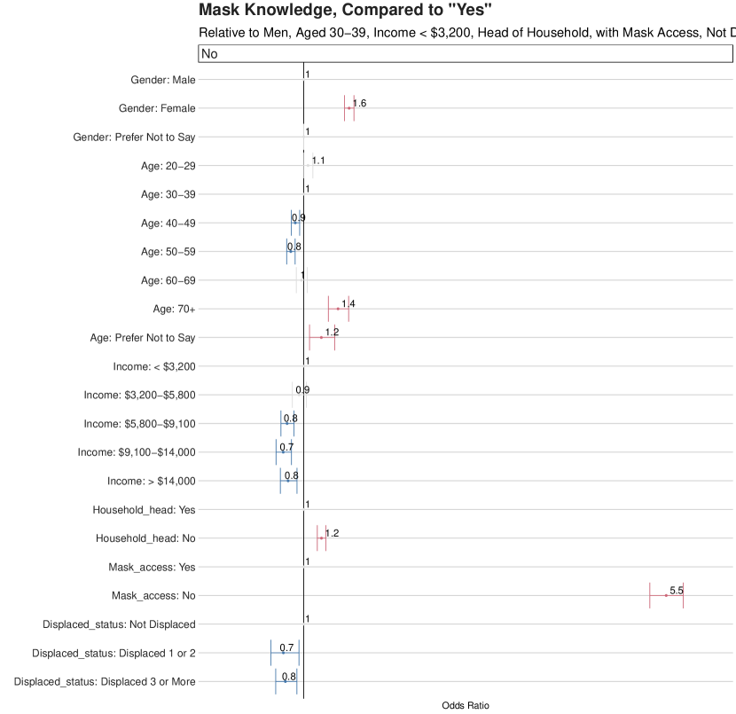
Figure 9: Odds ratio for not knowing whether a mask is effective, compared to knowing, adjusted for age, gender, income, mask access, and duration displaced. People without mask access have 5.5 times the odds of not knowing whether a mask is effective; controlling for that, women have 1.6 times the odds of not knowing. Values presented in Appendix Table LABEL:Total_weights_q29_mask_knowledge_regression_no_interaction_with_mask_access_income_displacement.

8 Discussion

8.1 Implications

We find that the combination of survey data and location data can provide a rich set of conclusions stronger than the strict sum of their parts. Mobility data alone fails to provide proper context for many findings. We would not, for example, understand the reasons for observed differences in displacement by gender and would be unable to use this information to inform policy response based solely on mobility data. Conversely, survey data alone, without mobility data, gives no reliable indication of distance of displacement or direction of displacement. Mobility data also greatly increases the efficiency of collecting survey data by identifying populations of interest without the need to perform extensive on-the-ground survey preparatory work. Conversely, survey data can be used to improve and validate models based entirely mobility data, providing a source of self-reported truth to expose biases or validate successes of model-based approaches.

These studies can also help better inform policy responses to disasters. Understanding characteristics of affected persons can inform the degree to which responses are fiscal, material, or organizational in nature. Social support can be better designed to account for likely patterns of household displacement and separation. In this case we reach conclusions that can be used to inform precisely these responses for future disasters.

Finally, this study provides a case example of the effects of fire on displacement, offering an investigation into heterogeneity in responses by demographic characteristics. We find significant differences by gender and income on a variety of outcomes including evacuation timing, agency in evacuation decisions, and household separation. This work reinforces the idea that disasters have highly heterogeneous effects on the affected population.

8.2 Limitations

In 2020, it was estimated that 60% of Australians were on Facebook or approximately 25 million individuals. Surveys always have limitations due to sampling frame (address, phone, social media), non-response and measurement Groves and Lyberg (2010). We have carefully reweighted the data for non-response and have no reason to expect this population to not be Representative of Facebook users. While this sampling frame does not cover all of Australia the general composition of Facebook users is not radically different than the full population (e.g., the age distribution looks comparable to full age distribution).

Interpretation of the household hypothesis could be influenced by the asymmetry of the questions, as the departure question asks about “anyone” staying behind whereas the return question refers to “you” the respondent. In future surveys we will update these questions to be consistent with one another.

Head of household is based on the respondent’s answer to the question: “Do you earn the most money among people in your household?” We acknowledge that this is a limited viewpoint on who leads a household. This is likely a poor definition in cases where earners travel away from their household for employment and send back financial support to a partner who, while not the primary income earner, is primarily responsible for day-to-day decision making and leadership within the family. In future surveys we can design a question more directly targeted to assessing this head of household designation.

8.3 Conclusion

Trends we had previously observed in Displacement Map data, such as women evacuating closer to home and men returning home from displacement sooner, were supported by this survey data. In addition to recognizing these qualitative similarities, we intend to use this data for a detailed assessment of the methodology underlying the Displacement map and make adjustments there if needed.

Gender differences remain an important area of research for us, as men and women face different challenges and needs when displaced. If men are returning faster than women, as both our displacement maps and surveys have shown, our humanitarian partners could consider using this information to plan their operations differently. Additionally, governments may want to rethink how they design and communicate evacuation orders in order to empower women to make evacuation decisions independently. Last, while our survey questions about mask access and knowledge were in the context of wildfire smoke, in a time of global pandemic where masks play a pivotal role in preventing spread of disease, governments and humanitarian organizations should make sure that there are no gender disparities in both the access and correct use of masks.

Appendix

Tables for Regression Models

Prevent Working Regression: Model With Income and Displacement Duration, No Interactions

Table 2: Prevent working, compared to “no”; relative to men, aged 30-39, income less than $3,200 head of household, not displaced based on model with main effects for age, gender, income, head of household, and duration displaced with no interactions

Response	Covariate	Odds Ratio	95% CI	P Value	Significance
Yes	Gender: Male	1.00
Yes	Gender: Female	0.91	(0.68, 1.2)	0.542
Yes	Gender: Prefer Not to Say	1.00	(1.00, 1.0)	NaN
Yes	Age: 20-29	1.42	(0.96, 2.1)	0.082	.
Yes	Age: 30-39	1.00
Yes	Age: 40-49	1.05	(0.69, 1.6)	0.826
Yes	Age: 50-59	1.07	(0.64, 1.8)	0.802
Yes	Age: 60-69	0.27	(0.14, 0.5)	0.000	***
Yes	Age: 70+	0.58	(0.25, 1.3)	0.184
Yes	Age: Prefer Not to Say	1.55	(0.52, 4.6)	0.437
Yes	Income: $<$ $3,200	1.00
Yes	Income: $3,200-$5,800	1.66	(0.86, 3.2)	0.131
Yes	Income: $5,800-$9,100	0.68	(0.34, 1.4)	0.276
Yes	Income: $9,100-$14,000	2.20	(0.69, 7.0)	0.183
Yes	Income: $>$ $14,000	0.88	(0.32, 2.4)	0.798
Yes	Income: Prefer Not to Say	0.47	(0.28, 0.8)	0.006	**
Yes	Household_head: Yes	1.00
Yes	Household_head: No	1.21	(0.88, 1.7)	0.242
Yes	Displaced_status: Displaced 1-3 nights	1.00
Yes	Displaced_status: Displaced more than 3 nights	1.79	(1.35, 2.4)	0.000	***

More than One Night Regression: Model With Income, No Interactions

Table 3: Displaced more than one night, compared to “yes”; relative to men, aged 30-39, income less than $3,200 head of household based on model with main effects for age, gender, income, and head of household with no interactions

Response	Covariate	Odds Ratio	95% CI	P Value	Significance
No	Gender: Male	1.00
No	Gender: Female	0.92	(0.80, 1.1)	0.266
No	Gender: Prefer Not to Say	1.00	(1.00, 1.0)	NaN
No	Age: 20-29	0.82	(0.68, 1.0)	0.043	*
No	Age: 30-39	1.00
No	Age: 40-49	0.95	(0.77, 1.2)	0.601
No	Age: 50-59	1.52	(1.19, 2.0)	0.001	***
No	Age: 60-69	1.30	(0.98, 1.7)	0.069	.
No	Age: 70+	1.07	(0.73, 1.6)	0.737
No	Age: Prefer Not to Say	0.76	(0.50, 1.2)	0.216
No	Income: $<$ $3,200	1.00
No	Income: $3,200-$5,800	1.43	(1.04, 2.0)	0.026	*
No	Income: $5,800-$9,100	1.87	(1.30, 2.7)	0.001	***
No	Income: $9,100-$14,000	1.86	(1.13, 3.1)	0.015	*
No	Income: $>$ $14,000	2.16	(1.30, 3.6)	0.003	**
No	Income: Prefer Not to Say	1.90	(1.46, 2.5)	0.000	***
No	Household_head: Yes	1.00
No	Household_head: No	1.32	(1.12, 1.5)	0.001	***

Household Split Return Regression: Model With Child Count, No Interactions

Table 4: Return home sooner, compared to “no”; relative to university educated women, aged 30-39, not head of household, with no children based on model with main effects for age, gender, education, and head of household with no interactions

Response	Covariate	Odds Ratio	95% CI	P Value	Significance
Yes	Gender: Male	2.07	(1.51, 2.9)	0.000	***
Yes	Gender: Female	1.00
Yes	Gender: Prefer Not to Say	1.00	(NaN, NaN)	NaN
Yes	Age: 20-29	1.19	(0.75, 1.9)	0.462
Yes	Age: 30-39	1.00
Yes	Age: 40-49	1.36	(0.87, 2.1)	0.182
Yes	Age: 50-59	2.10	(1.19, 3.7)	0.011	*
Yes	Age: 60-69	0.62	(0.28, 1.4)	0.246
Yes	Age: 70+	2.50	(1.07, 5.9)	0.035	*
Yes	Age: Prefer Not to Say	1.80	(0.73, 4.4)	0.202
Yes	Education: Elementary	0.48	(0.04, 5.7)	0.564
Yes	Education: Junior High	0.48	(0.15, 1.5)	0.216
Yes	Education: High School	0.39	(0.21, 0.7)	0.004	**
Yes	Education: Community College	0.34	(0.18, 0.7)	0.001	**
Yes	Education: University	1.00
Yes	Education: Graduate School	0.09	(0.03, 0.2)	0.000	***
Yes	Education: Prefer Not to Say	0.51	(0.20, 1.3)	0.149
Yes	Household_head: Yes	2.38	(1.66, 3.4)	0.000	***
Yes	Household_head: No	1.00
Yes	Any_children: FALSE	1.00
Yes	Any_children: TRUE	1.65	(1.17, 2.3)	0.004	**

Mask Knowledge Regression: Model With Mask Access, Income, and Displacement Duration, No Interactions

Table 5: Mask knowledge, compared to “yes”; relative to men, aged 30-39, income less than $3,200, head of household, with mask access, not displaced based on model with main effects for age, gender, income, head of household, and duration displaced with no interactions

Response	Covariate	Odds Ratio	95% CI	P Value	Significance
No	Gender: Male	1.00
No	Gender: Female	1.56	(1.50, 1.6)	0.000	***
No	Gender: Prefer Not to Say	1.00	(1.00, 1.0)	1.000
No	Age: 20-29	1.05	(1.00, 1.1)	0.068	.
No	Age: 30-39	1.00
No	Age: 40-49	0.90	(0.84, 0.9)	0.000	***
No	Age: 50-59	0.84	(0.79, 0.9)	0.000	***
No	Age: 60-69	0.97	(0.91, 1.0)	0.425
No	Age: 70+	1.42	(1.30, 1.6)	0.000	***
No	Age: Prefer Not to Say	1.22	(1.07, 1.4)	0.003	**
No	Income: $<$ $3,200	1.00
No	Income: $3,200-$5,800	0.94	(0.86, 1.0)	0.201
No	Income: $5,800-$9,100	0.79	(0.72, 0.9)	0.000	***
No	Income: $9,100-$14,000	0.75	(0.66, 0.8)	0.000	***
No	Income: $>$ $14,000	0.81	(0.71, 0.9)	0.001	***
No	Household_head: Yes	1.00
No	Household_head: No	1.22	(1.17, 1.3)	0.000	***
No	Mask_access: Yes	1.00
No	Mask_access: No	5.48	(5.27, 5.7)	0.000	***
No	Displaced_status: Not Displaced	1.00
No	Displaced_status: Displaced 1-3 nights	0.75	(0.59, 0.9)	0.013	*
No	Displaced_status: Displaced more than 3 nights	0.77	(0.65, 0.9)	0.003	**

Evacuation Decision Regression: Model with No Interactions

Table 6: Evacuation decision made by someone else, compared to “my decision”; relative to university educated men, aged 30-39, head of household based on model with main effects for age, gender, education, and head of household with no interactions

Response	Covariate	Odds Ratio	95% CI	P Value	Significance
Family Member	Gender: Male	1.00
Family Member	Gender: Female	1.28	(0.91, 1.8)	0.149
Family Member	Age: 20-29	2.28	(1.48, 3.5)	0.000	***
Family Member	Age: 30-39	1.00
Family Member	Age: 40-49	1.57	(0.95, 2.6)	0.077	.
Family Member	Age: 50-59	0.71	(0.36, 1.4)	0.314
Family Member	Age: 60-69	0.33	(0.11, 1.0)	0.052	.
Family Member	Age: 70+	1.74	(0.67, 4.5)	0.252
Family Member	Education: Elementary	2.58	(0.48, 13.7)	0.267
Family Member	Education: Junior High	2.25	(0.65, 7.8)	0.201
Family Member	Education: High School	1.58	(0.78, 3.2)	0.204
Family Member	Education: Community College	0.79	(0.35, 1.8)	0.567
Family Member	Education: University	1.00
Family Member	Education: Graduate School	2.01	(0.93, 4.4)	0.077	.
Family Member	Household_head: Yes	1.00
Family Member	Household_head: No	2.03	(1.40, 2.9)	0.000	***
Government	Gender: Male	1.00
Government	Gender: Female	2.34	(1.68, 3.3)	0.000	***
Government	Age: 20-29	1.77	(1.13, 2.8)	0.013	*
Government	Age: 30-39	1.00
Government	Age: 40-49	1.92	(1.19, 3.1)	0.007	**
Government	Age: 50-59	0.94	(0.51, 1.7)	0.832
Government	Age: 60-69	1.87	(1.01, 3.5)	0.048	*
Government	Age: 70+	3.21	(1.41, 7.3)	0.005	**
Government	Education: Elementary	2.23	(0.49, 10.2)	0.301
Government	Education: Junior High	1.51	(0.41, 5.5)	0.536
Government	Education: High School	0.55	(0.26, 1.2)	0.115
Government	Education: Community College	1.57	(0.81, 3.0)	0.178
Government	Education: University	1.00
Government	Education: Graduate School	0.78	(0.34, 1.8)	0.545
Government	Household_head: Yes	1.00
Government	Household_head: No	0.65	(0.45, 0.9)	0.022	*

Mask Access Regression: Model with No Interactions

Table 7: Mask access, compared to “yes”; relative to university educated men, aged 30-39, head of household based on model with main effects for age, gender, education, and head of household with no interactions

Response	Covariate	Odds Ratio	95% CI	P Value	Significance
No	Gender: Male	1.00
No	Gender: Female	1.37	(1.33, 1.4)	0.000	***
No	Gender: Prefer Not to Say	1.00	(1.00, 1.0)	NaN
No	Age: 20-29	0.88	(0.83, 0.9)	0.000	***
No	Age: 30-39	1.00
No	Age: 40-49	1.00	(0.94, 1.1)	1.000
No	Age: 50-59	1.02	(0.96, 1.1)	0.504
No	Age: 60-69	0.97	(0.91, 1.0)	0.393
No	Age: 70+	1.17	(1.07, 1.3)	0.000	***
No	Age: Prefer Not to Say	0.82	(0.73, 0.9)	0.002	**
No	Education: Elementary	2.37	(1.92, 2.9)	0.000	***
No	Education: Junior High	1.56	(1.35, 1.8)	0.000	***
No	Education: High School	1.27	(1.18, 1.4)	0.000	***
No	Education: Community College	0.97	(0.89, 1.0)	0.366
No	Education: University	1.00
No	Education: Graduate School	0.80	(0.74, 0.9)	0.000	***
No	Education: Prefer Not to Say	1.07	(0.97, 1.2)	0.185
No	Household_head: Yes	1.00
No	Household_head: No	0.96	(0.92, 1.0)	0.047	*

Supplementary Analysis

(a) Displaced More than One Night Overall

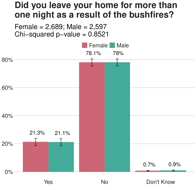
(b) Displaced More than One Night by Gender

Figure 10: The percent of people displaced for more than one night, among people who reported being in the affected region at the time of the fire.

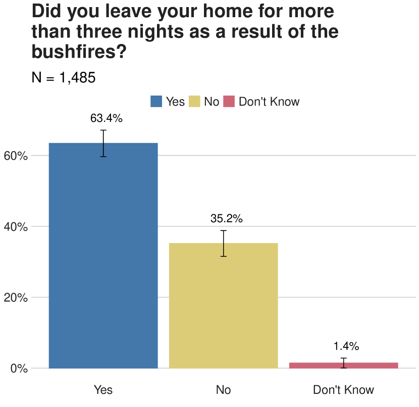
(a) Displaced More than Three Nights Overall

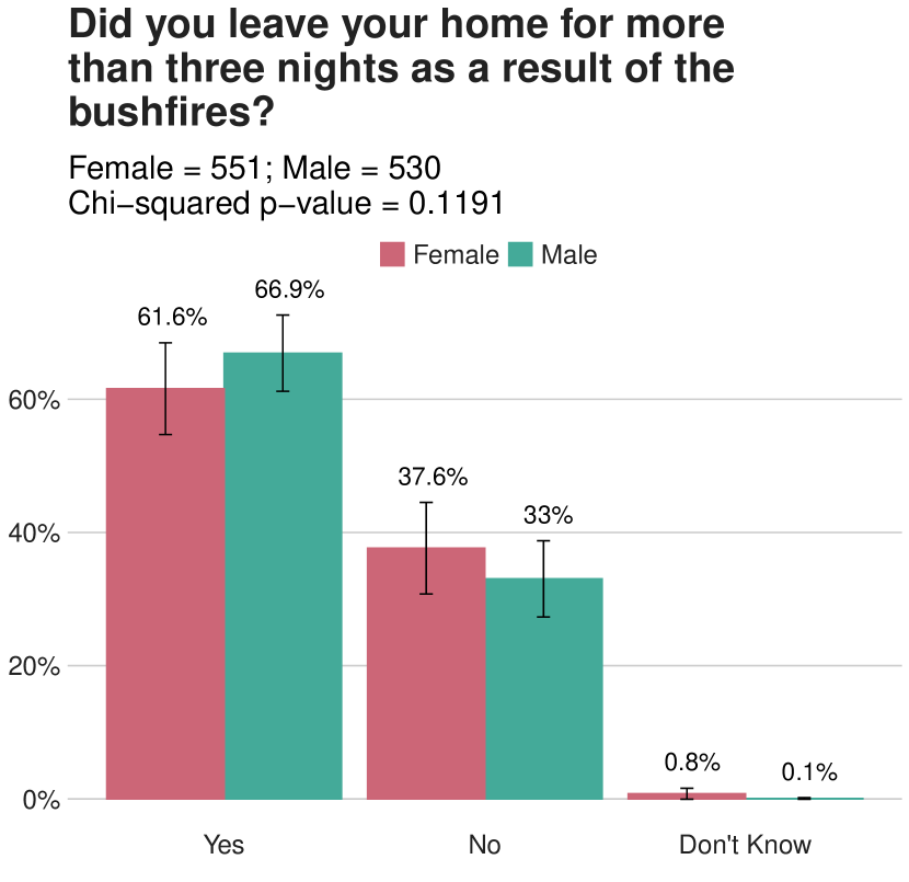
(b) Displaced More than Three Nights by Gender

Figure 11: The percent of people displaced for more than three nights, among people who reported being displaced more than one night.

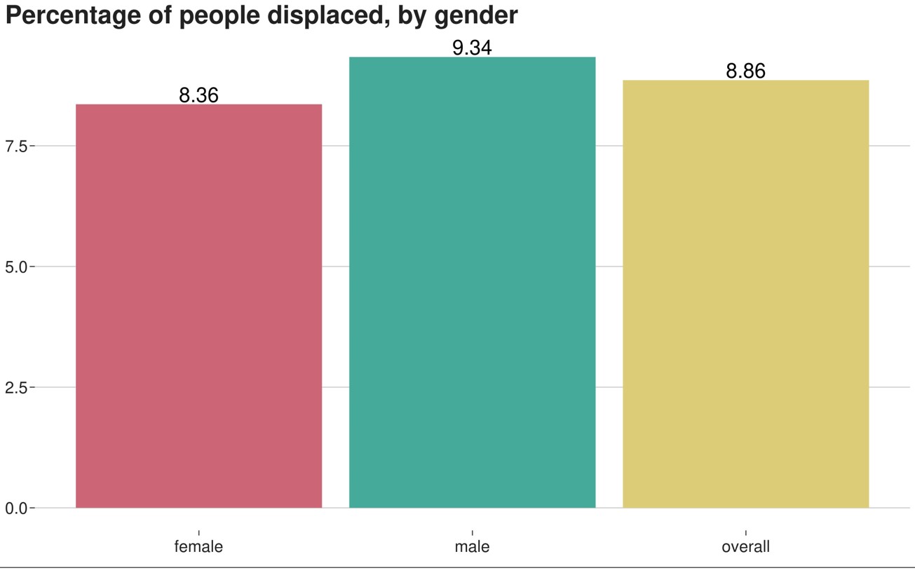
Figure 12: Percentage of people displaced, overall and by gender; estimated on aggregated and de-identified data from people who are using Facebook on their devices and have opted in to Location History.

^{https://research.fb.com/blog/2020/03/introducing-facebooks-gender-disaggregated-displacement-maps/}

(a) Left home more than three nights before the fire, by gender

(b) Left home before the fire, by gender

Figure 13: Women report leaving their homes ahead of the fire more often, and earlier than men do.

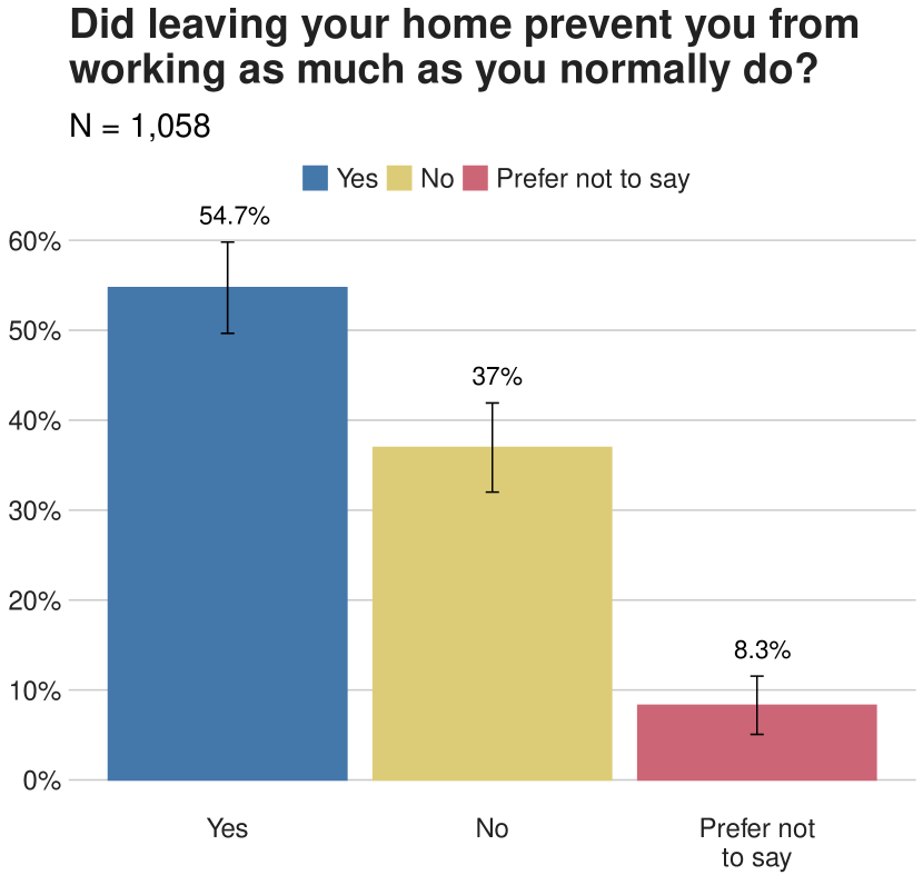
(a) Prevented from working, by overall

(b) Prevented from working, by gender

Figure 14: Proportion of people who responded that leaving home prevented them from working as much as usual.

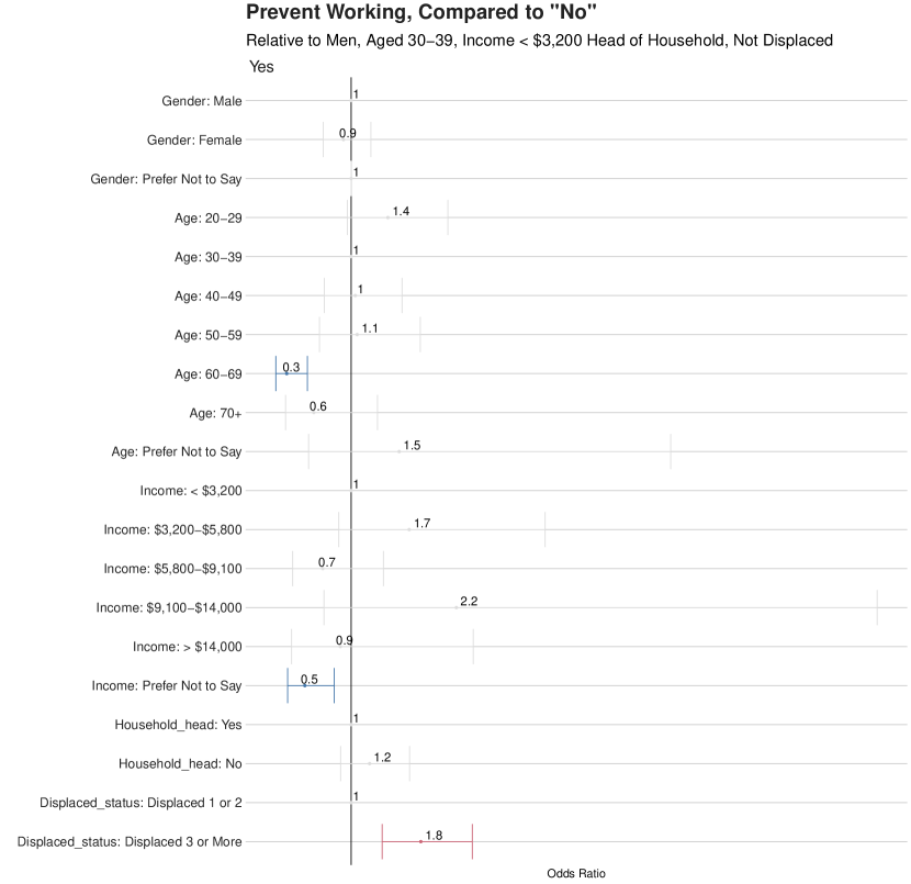
Figure 15: People who are displaced more than three nights are much more likely to say they were prevented from working. Values presented in Appendix Table LABEL:Total_weights_q21_prevent_working_regression_no_interaction_with_income_displacement_reformulated.

(a) Why Not Returned Home, Overall

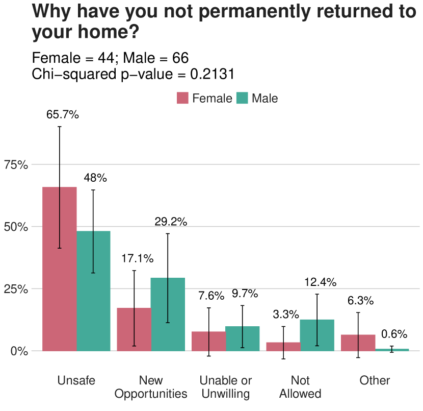
(b) Why Not Returned Home, by Gender

Figure 16: The primary reason that people do not return home is that it is still unsafe; however, a substantial fraction have found new opportunities.

The Survey Instrument

This section includes a diagram of the survey flow (Figure 19), and the survey instrument itself (Page 37).

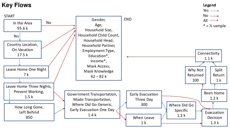
Figure 19: Diagram of the survey flow. Numbers give the approximate number of people who answered the question. These will not match the later counts exactly.

See pages - of au_bushfire_survey.pdf

Summaries by Question

Reported Gender - What is your gender?

Response	N
Female	42230
Male	35717

Table 8: Reported Gender: Weighted N, Overall and by Gender

Response	Percent
Female	54.2 (53.6, 54.7)
Male	45.8 (45.3, 46.4)

Table 9: Reported Gender: Percent, Overall and by Gender

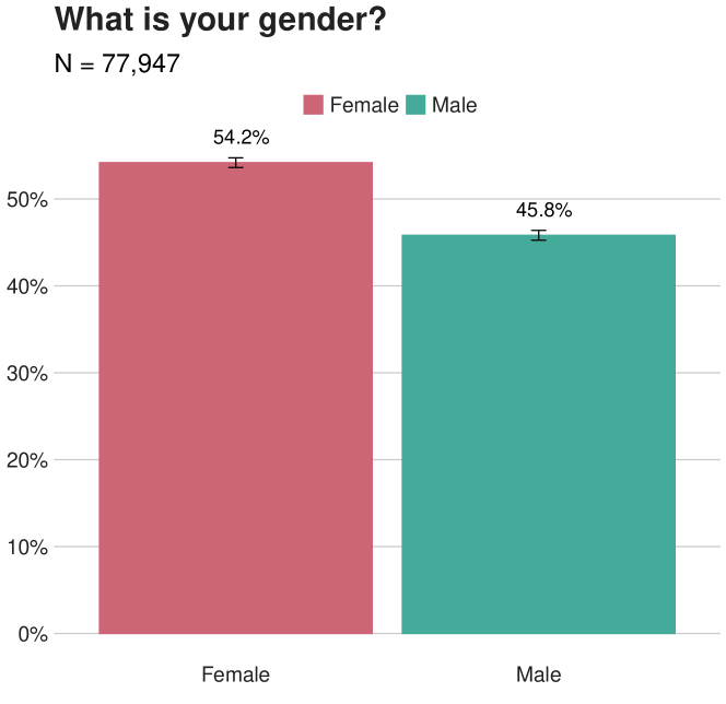
Figure 20: Reported Gender Overall

Reported Age - How old are you?

Response	Overall	Female	Male
$<$20	6171	3271	2712
20-29	17984	9384	8240
30-39	16200	8368	7583
40-49	12971	6714	5995
50-59	10692	5952	4607
60-69	7785	4277	3366
70+	4643	2508	1921
Prefer Not to Say	3200	1040	476

Table 10: Reported Age: Weighted N, Overall and by Gender

Response	Overall	Female	Male
$<$20	7.7 ( 7.4, 8.1)	7.9 ( 7.4, 8.3)	7.8 ( 7.3, 8.3)
20-29	22.6 (22.2, 23.0)	22.6 (22.0, 23.2)	23.6 (22.9, 24.3)
30-39	20.3 (19.9, 20.8)	20.2 (19.6, 20.7)	21.7 (21.0, 22.4)
40-49	16.3 (15.9, 16.7)	16.2 (15.6, 16.7)	17.2 (16.5, 17.9)
50-59	13.4 (13.0, 13.8)	14.3 (13.8, 14.8)	13.2 (12.6, 13.8)
60-69	9.8 ( 9.4, 10.1)	10.3 ( 9.8, 10.8)	9.6 ( 9.1, 10.2)
70+	5.8 ( 5.5, 6.1)	6.0 ( 5.7, 6.4)	5.5 ( 5.0, 6.0)
Prefer Not to Say	4.0 ( 3.8, 4.3)	2.5 ( 2.2, 2.8)	1.4 ( 1.1, 1.6)

Table 11: Reported Age: Percent, Overall and by Gender

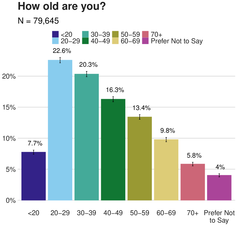
(a) Reported Age Overall

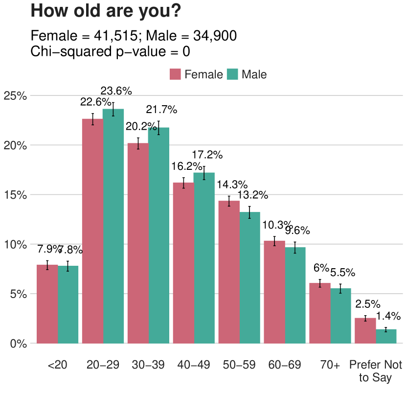
(b) Reported Age by Gender

Figure 21: How old are you?

Education - What is your highest level of completed education?

Response	Overall	Female	Male
Elementary	663	246	363
Junior High	1291	674	572
High School	9417	4990	4255
Community College	6996	3603	3282
University	5554	3125	2343
Graduate School	4750	2469	2114
Prefer Not to Say	3711	1762	1526

Table 12: Education: Weighted N, Overall and by Gender

Response	Overall	Female	Male
Elementary	2.0 ( 1.7, 2.4)	1.5 ( 1.0, 1.9)	2.5 ( 1.9, 3.1)
Junior High	4.0 ( 3.6, 4.4)	4.0 ( 3.5, 4.5)	4.0 ( 3.4, 4.5)
High School	29.1 (28.3, 29.9)	29.6 (28.5, 30.6)	29.4 (28.2, 30.7)
Community College	21.6 (20.9, 22.3)	21.4 (20.5, 22.2)	22.7 (21.6, 23.8)
University	17.2 (16.5, 17.8)	18.5 (17.6, 19.4)	16.2 (15.2, 17.2)
Graduate School	14.7 (14.1, 15.3)	14.6 (13.9, 15.4)	14.6 (13.7, 15.6)
Prefer Not to Say	11.5 (10.9, 12.1)	10.4 ( 9.7, 11.1)	10.6 ( 9.6, 11.5)

Table 13: Education: Percent, Overall and by Gender

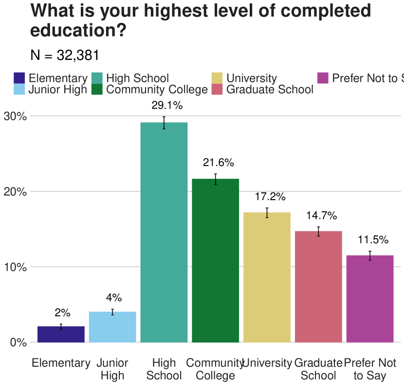
(a) Education Overall

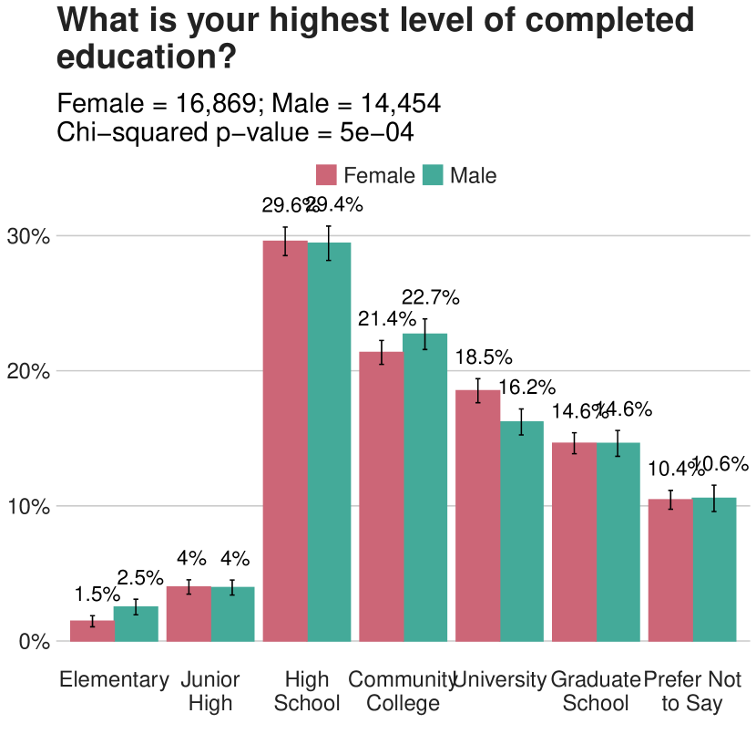
(b) Education by Gender

Figure 22: What is your highest level of completed education?

Employment Type - Which of the following best describes your main employment situation as of Dec. 18, 2019 when the bushfire started?

Response	Overall	Female	Male
Managing a Business	5506	2204	3184
Employed by Business	25350	12493	12484
Employed, not by Business	2686	1465	1167
Government Work	5983	3649	2206
Student	5329	2917	2251
Retired	7898	4377	3318
Not Working	7689	4785	2713
Prefer Not to Say	8484	4616	2932

Table 14: Employment Type: Weighted N, Overall and by Gender

Response	Overall	Female	Male
Managing a Business	8.0 ( 7.7, 8.3)	6.0 ( 5.7, 6.4)	10.5 (10.0, 11.1)
Employed by Business	36.8 (36.2, 37.3)	34.2 (33.5, 34.9)	41.3 (40.4, 42.2)
Employed, not by Business	3.9 ( 3.7, 4.1)	4.0 ( 3.7, 4.3)	3.9 ( 3.5, 4.2)
Government Work	8.7 ( 8.4, 9.0)	10.0 ( 9.6, 10.4)	7.3 ( 6.8, 7.8)
Student	7.7 ( 7.4, 8.1)	8.0 ( 7.5, 8.4)	7.4 ( 6.9, 7.9)
Retired	11.5 (11.0, 11.9)	12.0 (11.4, 12.5)	11.0 (10.3, 11.6)
Not Working	11.2 (10.7, 11.6)	13.1 (12.5, 13.7)	9.0 ( 8.3, 9.6)
Prefer Not to Say	12.3 (11.9, 12.7)	12.6 (12.1, 13.2)	9.7 ( 9.1, 10.3)

Table 15: Employment Type: Percent, Overall and by Gender

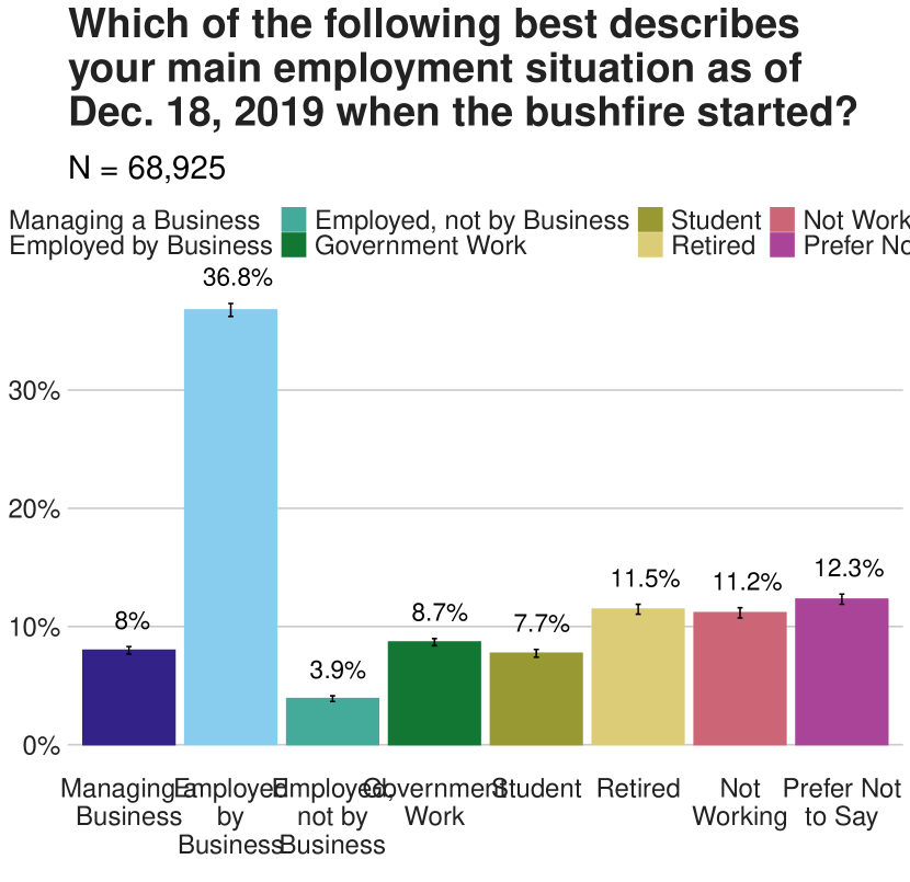
(a) Employment Type Overall

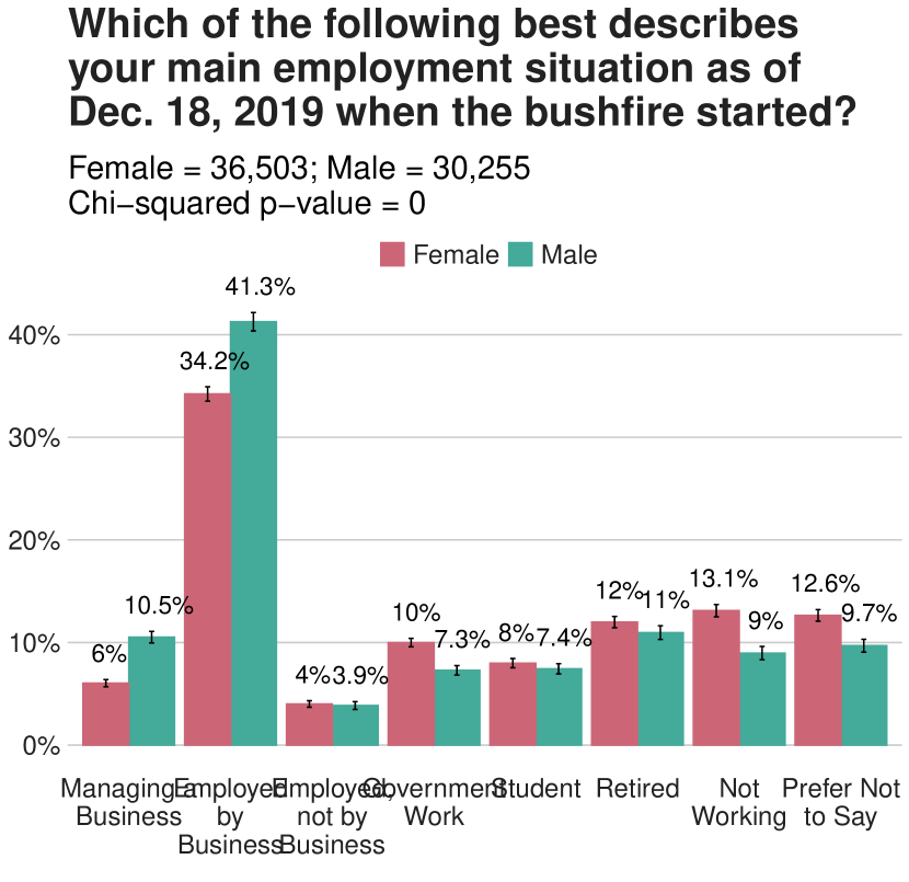
(b) Employment Type by Gender

Figure 23: Which of the following best describes your main employment situation as of Dec. 18, 2019 when the bushfire started?

Income - What was your total household income last month?

Response	Overall	Female	Male
$<$ $3,200	5892	3083	2668
$3,200-$5,800	4263	2185	2032
$5,800-$9,100	2877	1419	1421
$9,100-$14,000	1547	697	827
$>$ $14,000	1624	711	860
Prefer Not to Say	14918	8464	5775

Table 16: Income: Weighted N, Overall and by Gender

Response	Overall	Female	Male
$<$ $3,200	18.9 (18.1, 19.7)	18.6 (17.6, 19.6)	19.6 (18.4, 20.9)
$3,200-$5,800	13.7 (13.1, 14.3)	13.2 (12.4, 14.0)	15.0 (14.0, 15.9)
$5,800-$9,100	9.2 ( 8.8, 9.7)	8.6 ( 8.0, 9.1)	10.5 ( 9.7, 11.2)
$9,100-$14,000	5.0 ( 4.6, 5.3)	4.2 ( 3.8, 4.6)	6.1 ( 5.5, 6.7)
$>$ $14,000	5.2 ( 4.8, 5.6)	4.3 ( 3.8, 4.8)	6.3 ( 5.7, 7.0)
Prefer Not to Say	47.9 (47.0, 48.8)	51.1 (49.9, 52.3)	42.5 (41.1, 43.9)

Table 17: Income: Percent, Overall and by Gender

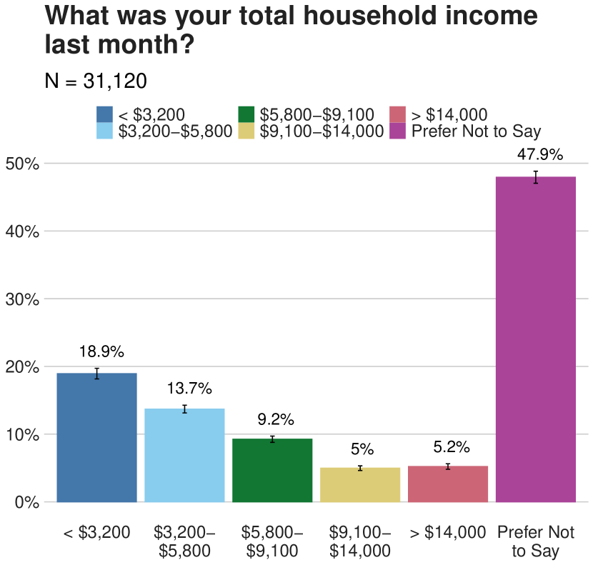
(a) Income Overall

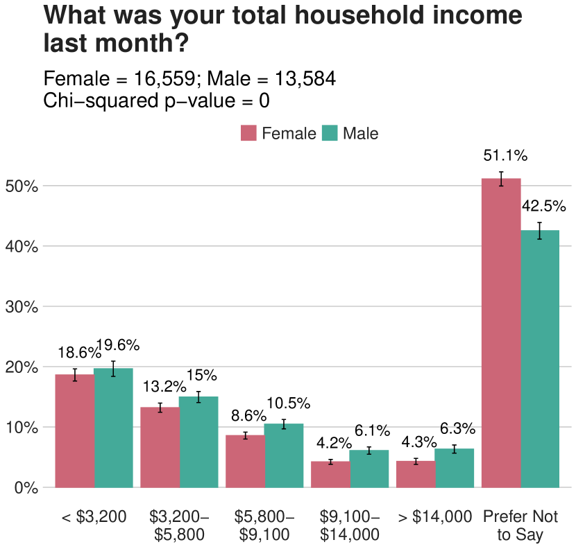
(b) Income by Gender

Figure 24: What was your total household income last month?

Country Location - Which area were you in on December 18, 2019 when the Australian bushfires began?

Response	Overall	Female	Male
The Green Wattle Creek Fire across Eastern New South Wales	4581	1901	1923
The Cudlee Creek Fire in Adelaide Hills, South Australia	1740	772	662

Table 18: Country Location: Weighted N, Overall and by Gender

Response	Overall	Female	Male
The Green Wattle Creek Fire across Eastern New South Wales	72.5 (70.8, 74.1)	71.1 (68.6, 73.6)	74.4 (71.7, 77.0)
The Cudlee Creek Fire in Adelaide Hills, South Australia	27.5 (25.9, 29.2)	28.9 (26.4, 31.4)	25.6 (23.0, 28.3)

Table 19: Country Location: Percent, Overall and by Gender

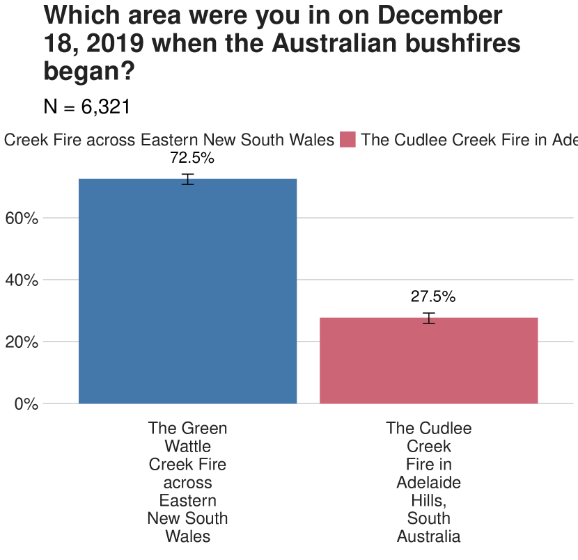
(a) Country Location Overall

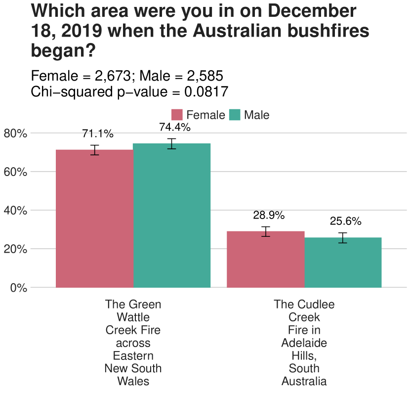
(b) Country Location by Gender

Figure 25: Which area were you in on December 18, 2019 when the Australian bushfires began?

Three Nights Before Fires - Did you leave more than 3 nights BEFORE the bushfire on December 18, 2019?

Response	Overall	Female	Male
Yes	104	49	30
No	176	49	94
Don’t Know	29	22	3

Table 20: Three Nights Before Fires: Weighted N, Overall and by Gender

Response	Overall	Female	Male
Yes	33.5 (25.3, 41.7)	41.2 (26.5, 55.9)	23.5 (13.5, 33.5)
No	57.0 (47.5, 66.5)	40.5 (25.2, 55.9)	73.9 (63.4, 84.4)
Don’t Know	9.5 ( 0.8, 18.2)	18.3 (-1.6, 38.2)	2.5 (-0.6, 5.7)

Table 21: Three Nights Before Fires: Percent, Overall and by Gender

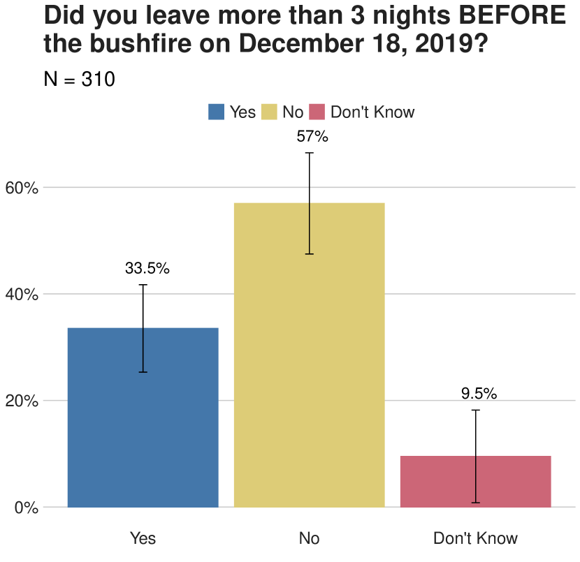
(a) Three Nights Before Fires Overall

(b) Three Nights Before Fires by Gender

Figure 26: Did you leave more than 3 nights BEFORE the bushfire on December 18, 2019?

Before Fires Evacuation - Did you leave your home BEFORE the bushfire on December 18, 2019?

Response	Overall	Female	Male
Yes	339	133	132
No	991	426	402
Don’t Know	45	12	13

Table 22: Before Fires Evacuation: Weighted N, Overall and by Gender

Response	Overall	Female	Male
Yes	24.7 (20.8, 28.6)	23.3 (16.6, 30.0)	24.1 (18.3, 30.0)
No	72.1 (68.1, 76.0)	74.6 (67.9, 81.4)	73.4 (67.5, 79.3)
Don’t Know	3.3 ( 2.2, 4.4)	2.1 ( 0.7, 3.5)	2.4 ( 1.1, 3.7)

Table 23: Before Fires Evacuation: Percent, Overall and by Gender

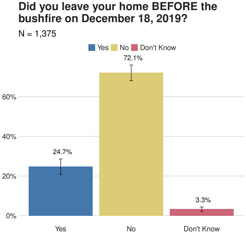
(a) Before Fires Evacuation Overall

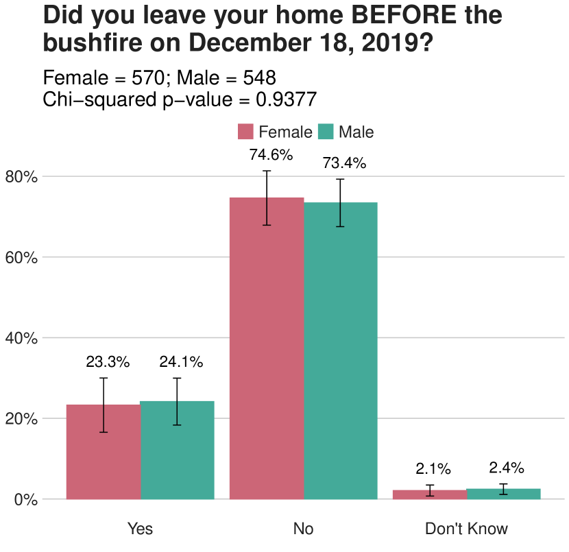
(b) Before Fires Evacuation by Gender

Figure 27: Did you leave your home BEFORE the bushfire on December 18, 2019?

Early Evacuation - Were you evacuated BEFORE the bushfire on December 18, 2019 by your local, state, or national government?

Response	Overall	Female	Male
Yes	339	133	132
No	991	426	402
Don’t Know	45	12	13

Table 24: Early Evacuation: Weighted N, Overall and by Gender

Response	Overall	Female	Male
Yes	24.7 (20.8, 28.6)	23.3 (16.6, 30.0)	24.1 (18.3, 30.0)
No	72.1 (68.1, 76.0)	74.6 (67.9, 81.4)	73.4 (67.5, 79.3)
Don’t Know	3.3 ( 2.2, 4.4)	2.1 ( 0.7, 3.5)	2.4 ( 1.1, 3.7)

Table 25: Early Evacuation: Percent, Overall and by Gender

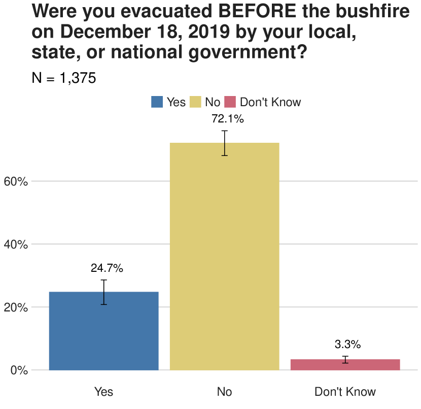
(a) Early Evacuation Overall

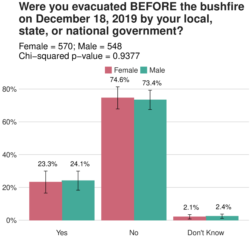
(b) Early Evacuation by Gender

Figure 28: Were you evacuated BEFORE the bushfire on December 18, 2019 by your local, state, or national government?

When Did You Leave Your Home - When did you leave your home?

Response	Overall	Female	Male
$<$7	486	209	218
7-14	229	112	94
$>$14	145	68	56
Don’t Know	129	50	47

Table 26: When Did You Leave Your Home: Weighted N, Overall and by Gender

Response	Overall	Female	Male
$<$7	49.2 (44.4, 54.0)	47.7 (40.2, 55.2)	52.5 (44.9, 60.0)
7-14	23.1 (18.9, 27.4)	25.5 (18.3, 32.6)	22.7 (16.7, 28.8)
$>$14	14.6 (11.7, 17.6)	15.5 (10.6, 20.3)	13.5 ( 9.3, 17.7)
Don’t Know	13.0 (10.4, 15.6)	11.4 ( 7.7, 15.0)	11.3 ( 7.5, 15.1)

Table 27: When Did You Leave Your Home: Percent, Overall and by Gender

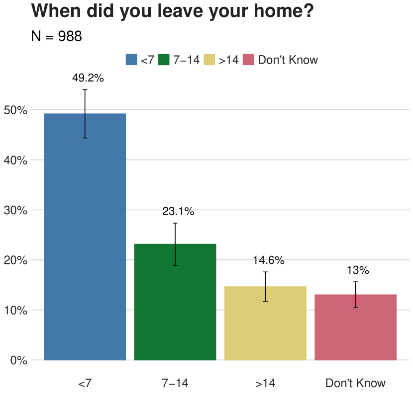
(a) When Did You Leave Your Home Overall

(b) When Did You Leave Your Home by Gender

Figure 29: When did you leave your home?

One Night - Did you leave your home for more than one night as a result of the bushfires?

Response	Overall	Female	Male
Yes	1566	572	548
No	4517	2099	2026
Don’t Know	65	18	23

Table 28: One Night: Weighted N, Overall and by Gender

Response	Overall	Female	Male
Yes	25.5 (23.8, 27.2)	21.3 (18.7, 23.8)	21.1 (18.6, 23.6)
No	73.5 (71.7, 75.2)	78.1 (75.5, 80.6)	78.0 (75.5, 80.6)
Don’t Know	1.1 ( 0.6, 1.5)	0.7 ( 0.3, 1.1)	0.9 ( 0.5, 1.3)

Table 29: One Night: Percent, Overall and by Gender

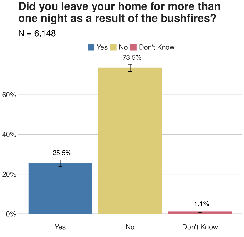
(a) One Night Overall

(b) One Night by Gender

Figure 30: Did you leave your home for more than one night as a result of the bushfires?

Three Nights - Did you leave your home for more than three nights as a result of the bushfires?

Response	Overall	Female	Male
Yes	942	339	355
No	522	207	175
Don’t Know	21	4	0

Table 30: Three Nights: Weighted N, Overall and by Gender

Response	Overall	Female	Male
Yes	63.4 (59.7, 67.1)	61.6 (54.7, 68.5)	66.9 (61.2, 72.6)
No	35.2 (31.5, 38.8)	37.6 (30.8, 44.5)	33.0 (27.3, 38.7)
Don’t Know	1.4 ( 0.0, 2.8)	0.8 ( 0.0, 1.6)	0.1 (-0.1, 0.2)

Table 31: Three Nights: Percent, Overall and by Gender

(a) Three Nights Overall

(b) Three Nights by Gender

Figure 31: Did you leave your home for more than three nights as a result of the bushfires?

Evacuation Decision - Whose decision first led you to leaving your home?

Response	Overall	Female	Male
Mine	606	212	294
Family Member	310	138	130
Government	301	172	109
Other	56	37	12

Table 32: Evacuation Decision: Weighted N, Overall and by Gender

Response	Overall	Female	Male
Mine	47.7 (43.3, 52.0)	37.9 (31.9, 43.9)	54.0 (47.2, 60.7)
Family Member	24.3 (20.6, 28.0)	24.7 (18.6, 30.7)	23.8 (18.3, 29.3)
Government	23.6 (19.4, 27.9)	30.8 (23.5, 38.1)	20.0 (14.3, 25.7)
Other	4.4 ( 3.1, 5.7)	6.6 ( 4.1, 9.1)	2.2 ( 1.0, 3.5)

Table 33: Evacuation Decision: Percent, Overall and by Gender

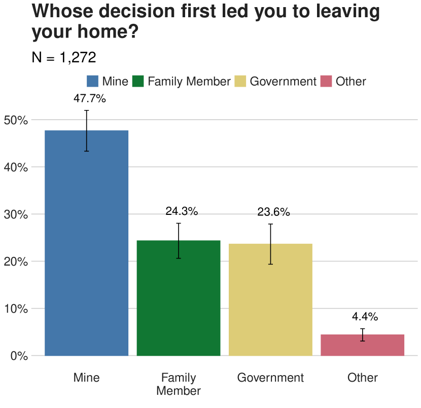
(a) Evacuation Decision Overall

(b) Evacuation Decision by Gender

Figure 32: Whose decision first led you to leaving your home?

Government Transportation - Did the government help you with transportation to leave your home?

Response	Overall	Female	Male
Yes	75	32	24
No	1262	490	496
Don’t Know	28	14	4

Table 34: Government Transportation: Weighted N, Overall and by Gender

Response	Overall	Female	Male
Yes	5.5 ( 3.0, 7.9)	6.0 ( 0.5, 11.5)	4.6 ( 2.5, 6.8)
No	92.5 (90.0, 95.0)	91.4 (85.8, 97.0)	94.6 (92.3, 96.8)
Don’t Know	2.0 ( 1.2, 2.9)	2.6 ( 0.9, 4.3)	0.8 ( 0.1, 1.5)

Table 35: Government Transportation: Percent, Overall and by Gender

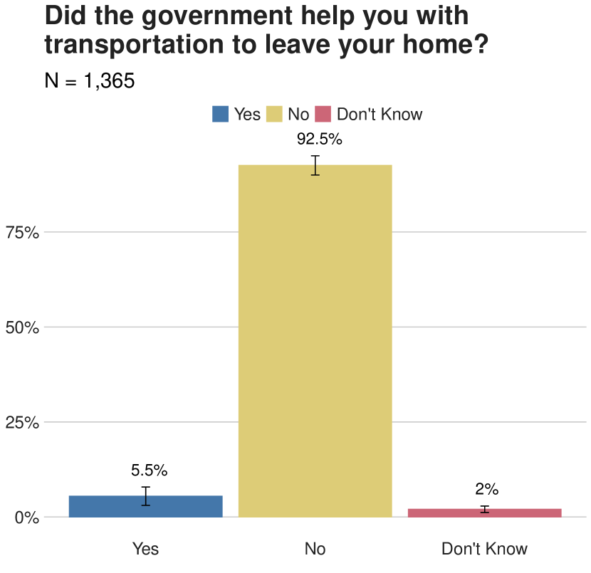
(a) Government Transportation Overall

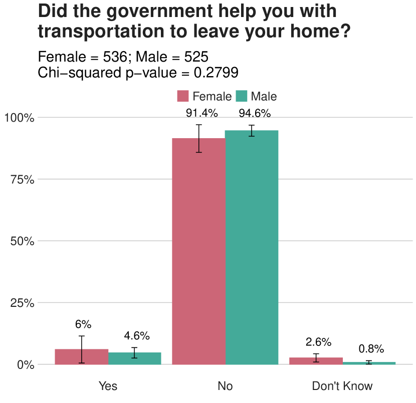
(b) Government Transportation by Gender

Figure 33: Did the government help you with transportation to leave your home?

Mode Transportation - What mode of transportation did you take when you left your home for more than one night as a result of the bushfires?

Response	Overall	Female	Male
Car	1268	526	491
Walking	50	7	24
Bus or Train	55	21	11
Bike	37	10	15
Other	15	3	5

Table 36: Mode Transportation: Weighted N, Overall and by Gender

Response	Overall	Female	Male
Car	89.0 (86.1, 91.8)	92.7 (87.7, 97.7)	89.9 (86.8, 93.0)
Walking	3.5 ( 2.4, 4.7)	1.3 ( 0.2, 2.3)	4.4 ( 2.3, 6.5)
Bus or Train	3.9 ( 1.6, 6.1)	3.6 (-0.5, 7.8)	2.1 ( 0.6, 3.5)
Bike	2.6 ( 1.2, 4.0)	1.8 (-1.0, 4.6)	2.7 ( 1.1, 4.3)
Other	1.1 ( 0.5, 1.7)	0.6 (-0.1, 1.3)	1.0 ( 0.2, 1.8)

Table 37: Mode Transportation: Percent, Overall and by Gender

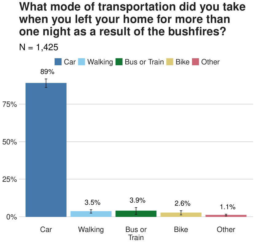
(a) Mode Transporation Overall

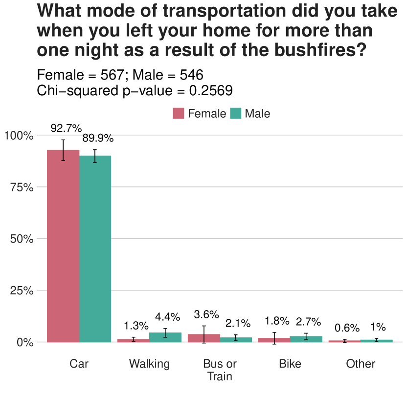
(b) Mode Transporation by Gender

Figure 34: What mode of transportation did you take when you left your home for more than one night as a result of the bushfires?

Leave Home Where Did Go - Where did you go when you left your home?

Response	Overall	Female	Male
Same City As Home	383	185	141
Different City in My Region	810	344	361
Different State	69	27	28
Other	15	0	10

Table 38: Leave Home Where Did Go: Weighted N, Overall and by Gender

Response	Overall	Female	Male
Same City As Home	30.0 (26.3, 33.8)	33.2 (27.0, 39.4)	26.1 (20.7, 31.5)
Different City in My Region	63.4 (59.4, 67.5)	61.8 (55.2, 68.5)	66.9 (61.1, 72.8)
Different State	5.4 ( 3.3, 7.4)	4.9 ( 1.1, 8.8)	5.2 ( 2.9, 7.4)
Other	1.2 ( 0.5, 1.9)	0.0 ( 0.0, 0.1)	1.8 ( 0.4, 3.1)

Table 39: Leave Home Where Did Go: Percent, Overall and by Gender

(a) Leave Home Where Did Go Overall

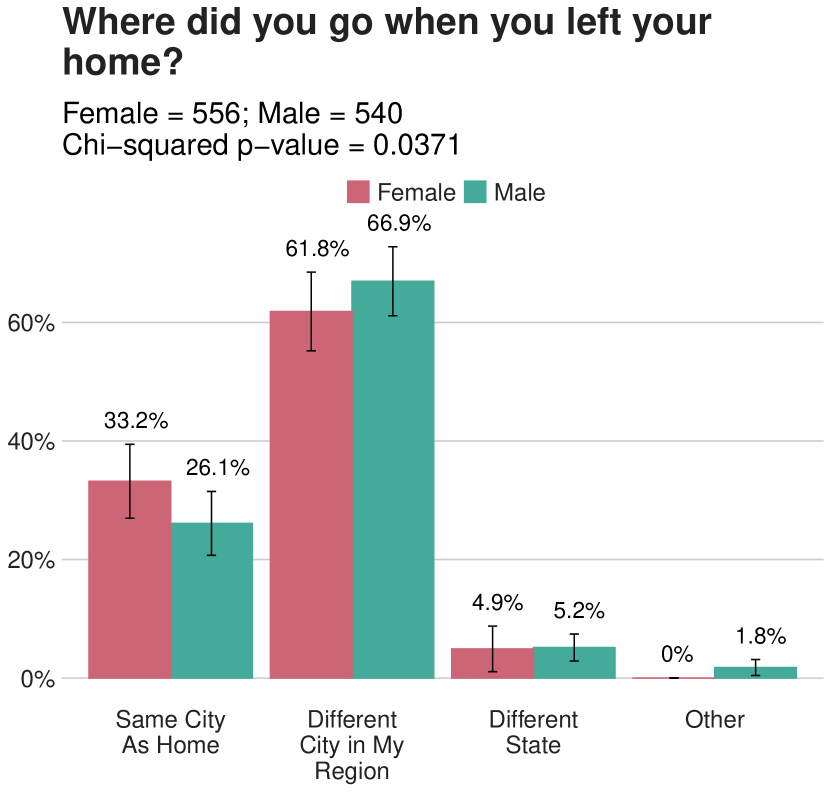
(b) Leave Home Where Did Go by Gender

Figure 35: Where did you go when you left your home?

Connectivity - While you were away from your home during the bushfires, did you consistently have access to mobile data or wifi on the main mobile device that you use?

Response	Overall	Female	Male
Yes	726	364	332
No	395	176	187
Don’t Know	34	12	15

Table 40: Connectivity: Weighted N, Overall and by Gender

Response	Overall	Female	Male
Yes	62.8 (58.5, 67.2)	66.0 (59.7, 72.3)	62.2 (55.8, 68.6)
No	34.2 (29.9, 38.5)	31.8 (25.6, 38.0)	34.9 (28.6, 41.3)
Don’t Know	2.9 ( 1.8, 4.1)	2.2 ( 0.8, 3.5)	2.9 ( 1.3, 4.5)

Table 41: Connectivity: Percent, Overall and by Gender

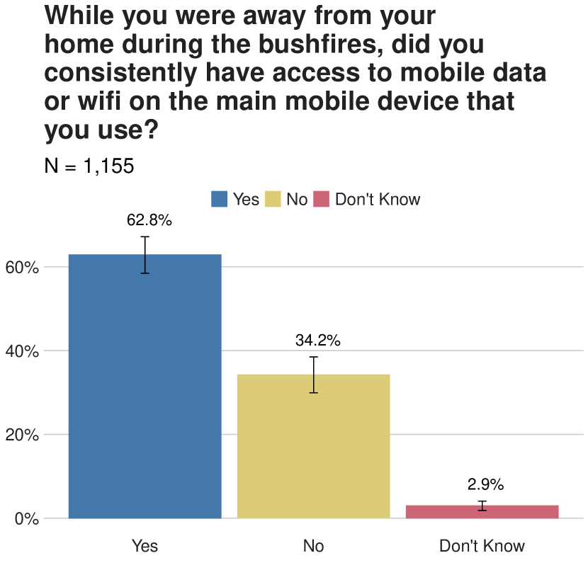
(a) Connectivity Overall

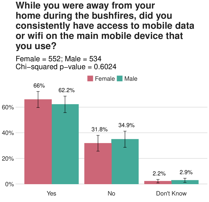
(b) Connectivity by Gender

Figure 36: While you were away from your home during the bushfires, did you consistently have access to mobile data or wifi on the main mobile device that you use?

How Long Gone In Total - How long, in total, were you away from your home as a result of the bushfires?

Response	Overall	Female	Male
$<$7	388	136	148
7-14	304	123	109
14-30	117	39	63
$>$30	84	34	28
Don’t Know	31	7	8

Table 42: How Long Gone In Total: Weighted N, Overall and by Gender

Response	Overall	Female	Male
$<$7	42.0 (37.0, 47.0)	40.1 (31.8, 48.5)	41.8 (33.1, 50.5)
7-14	32.9 (27.8, 38.0)	36.3 (26.6, 45.9)	30.6 (22.9, 38.2)
14-30	12.6 ( 8.0, 17.3)	11.6 ( 4.4, 18.8)	17.6 ( 8.3, 27.0)
$>$30	9.1 ( 5.8, 12.4)	10.1 ( 2.7, 17.6)	7.9 ( 4.3, 11.4)
Don’t Know	3.3 ( 2.0, 4.7)	1.9 ( 0.3, 3.6)	2.1 ( 0.3, 4.0)

Table 43: How Long Gone In Total: Percent, Overall and by Gender

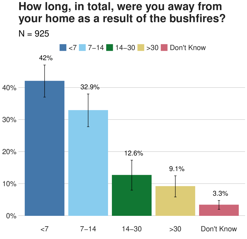
(a) How Long Gone In Total Overall

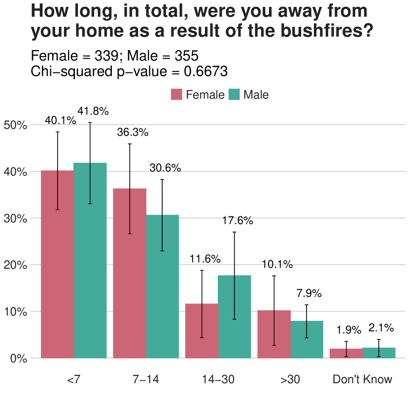
(b) How Long Gone In Total by Gender

Figure 37: How long, in total, were you away from your home as a result of the bushfires?

Been Home - Since you first left as a result of the bushfires have you been home for at least a total of 3 nights?

Response	Overall	Female	Male
Yes	1062	504	466
No	144	46	67
Don’t Know	28	8	8

Table 44: Been Home: Weighted N, Overall and by Gender

Response	Overall	Female	Male
Yes	86.1 (83.0, 89.1)	90.3 (85.5, 95.1)	86.1 (82.0, 90.2)
No	11.7 ( 8.7, 14.6)	8.2 ( 3.5, 13.0)	12.4 ( 8.4, 16.3)
Don’t Know	2.3 ( 1.3, 3.2)	1.5 ( 0.3, 2.7)	1.5 ( 0.4, 2.7)

Table 45: Been Home: Percent, Overall and by Gender

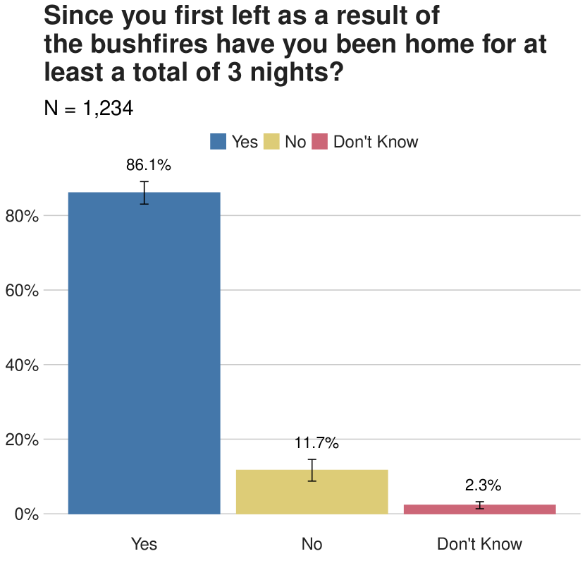
(a) Been Home Overall

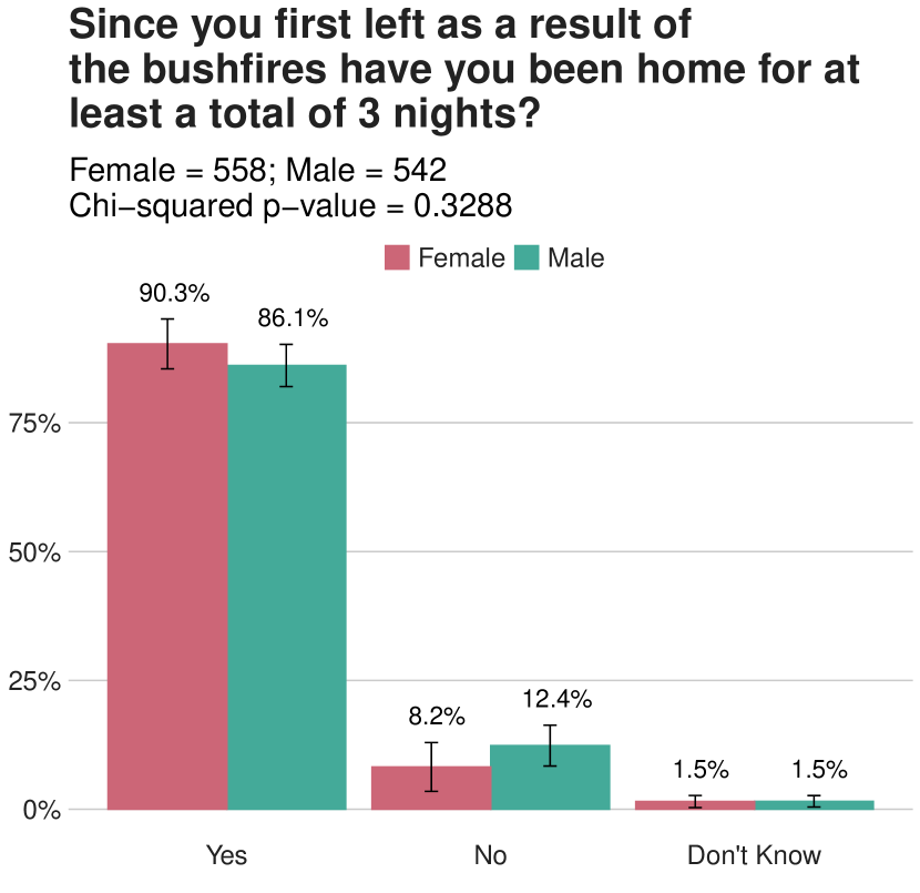
(b) Been Home by Gender

Figure 38: Since you first left as a result of the bushfires have you been home for at least a total of 3 nights?

Why Not Return Home - Why have you not permanently returned to your home?

Response	Overall	Female	Male
Unsafe	72	29	32
New Opportunities	28	7	19
Unable or Unwilling	12	3	6
Not Allowed	10	1	8
Other	3	3	0

Table 46: Why Not Return Home: Weighted N, Overall and by Gender

Response	Overall	Female	Male
Unsafe	57.5 (43.4, 71.5)	65.7 (41.3, 90.2)	48.0 (31.3, 64.7)
New Opportunities	22.2 (10.4, 34.1)	17.1 ( 1.9, 32.3)	29.2 (11.3, 47.1)
Unable or Unwilling	9.7 ( 3.3, 16.1)	7.6 (-2.1, 17.3)	9.7 ( 1.2, 18.2)
Not Allowed	8.0 ( 1.8, 14.3)	3.3 (-3.3, 9.8)	12.4 ( 2.0, 22.8)
Other	2.6 (-0.6, 5.7)	6.3 (-2.7, 15.4)	0.6 (-0.6, 1.9)

Table 47: Why Not Return Home: Percent, Overall and by Gender

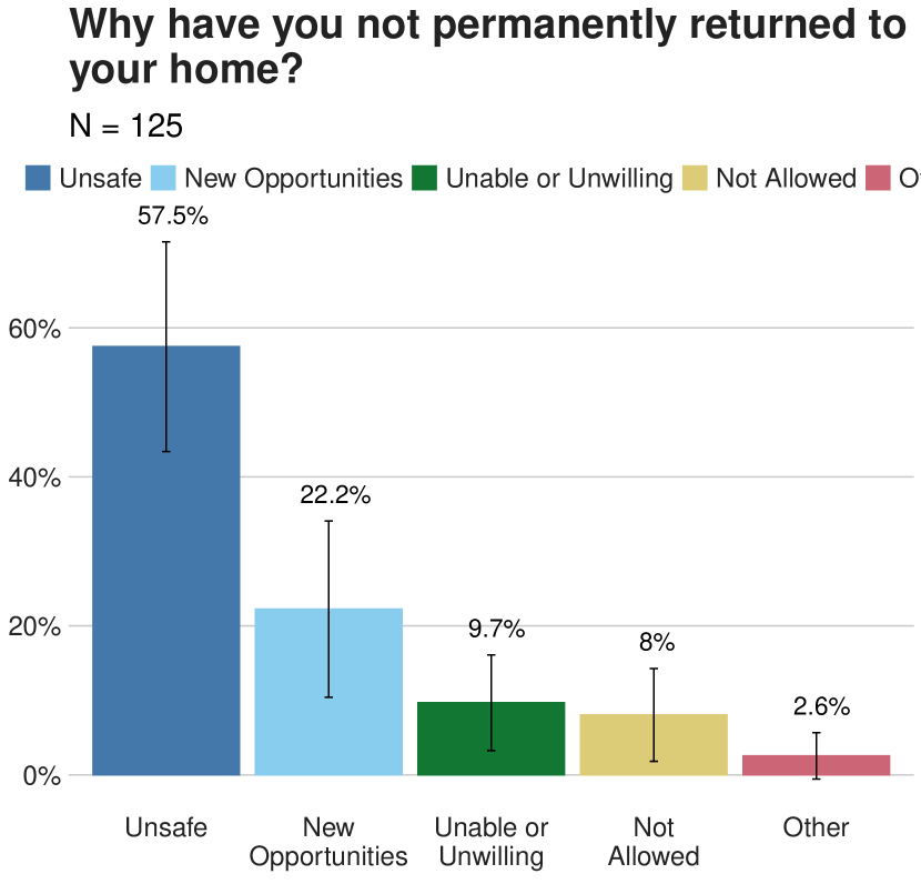
(a) Why Not Return Home Overall

(b) Why Not Return Home by Gender

Figure 39: Why have you not permanently returned to your home?

Prevent Working - Did leaving your home prevent you from working as much as you normally do?

Response	Overall	Female	Male
Yes	579	270	285
No	391	198	181
Prefer not to say	88	56	24

Table 48: Prevent Working: Weighted N, Overall and by Gender

Response	Overall	Female	Male
Yes	54.7 (49.7, 59.8)	51.5 (44.0, 59.0)	58.0 (50.8, 65.3)
No	37.0 (32.0, 41.9)	37.9 (30.6, 45.1)	37.0 (29.8, 44.2)
Prefer not to say	8.3 ( 5.1, 11.5)	10.7 ( 5.1, 16.2)	5.0 ( 1.6, 8.4)

Table 49: Prevent Working: Percent, Overall and by Gender

(a) Prevent Working Overall

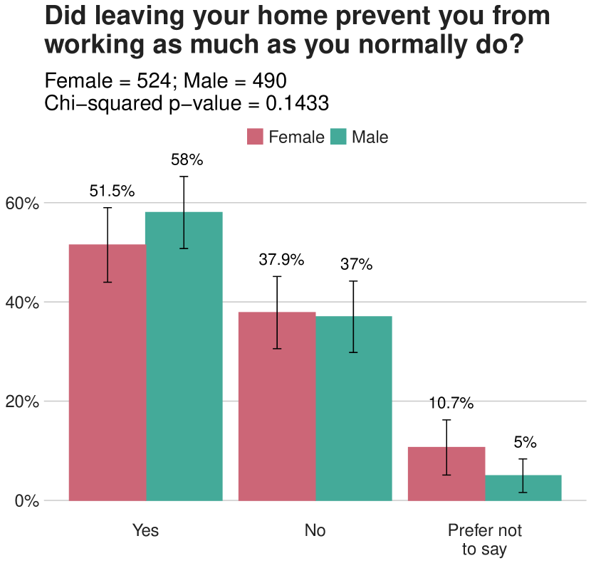
(b) Prevent Working by Gender

Figure 40: Did leaving your home prevent you from working as much as you normally do?

Household Head - Do you earn the most money among people in your household?

Response	Overall	Female	Male
Yes	24727	10262	14117
No	31150	19504	11037
Prefer not to say	15062	7798	5974

Table 50: Household Head: Weighted N, Overall and by Gender

Response	Overall	Female	Male
Yes	34.9 (34.3, 35.4)	27.3 (26.6, 28.0)	45.4 (44.4, 46.3)
No	43.9 (43.3, 44.5)	51.9 (51.2, 52.7)	35.5 (34.6, 36.3)
Prefer not to say	21.2 (20.7, 21.7)	20.8 (20.1, 21.4)	19.2 (18.5, 19.9)

Table 51: Household Head: Percent, Overall and by Gender

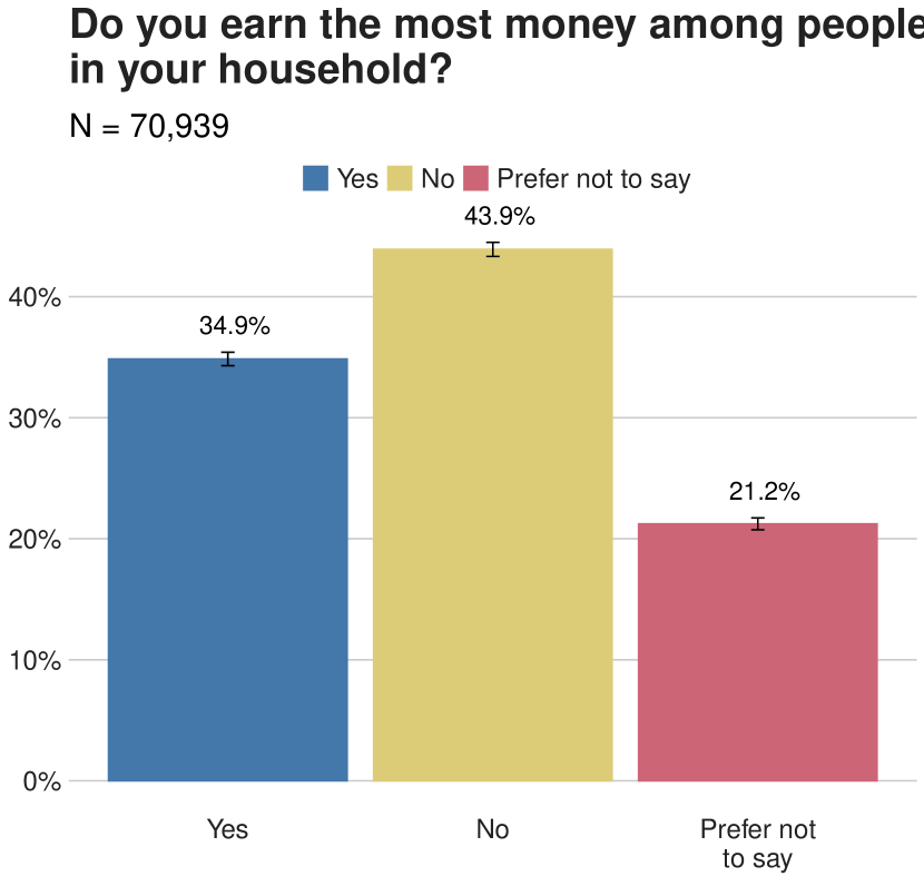
(a) Household Head Overall

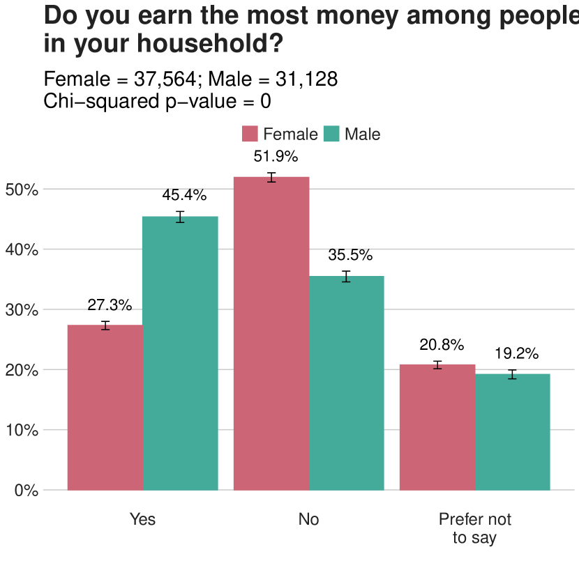
(b) Household Head by Gender

Figure 41: Do you earn the most money among people in your household?

Household Size - How many people live in your household (including yourself)?

Response	Overall	Female	Male
1	8964	4412	4244
2	20319	11211	8642
3	14392	7721	6313
4	14910	7928	6613
5	8197	4243	3748
6 or more	6360	3228	2621

Table 52: Household Size: Weighted N, Overall and by Gender

Response	Overall	Female	Male
1	12.3 (11.8, 12.7)	11.4 (10.8, 11.9)	13.2 (12.5, 13.9)
2	27.8 (27.3, 28.3)	28.9 (28.3, 29.6)	26.9 (26.1, 27.7)
3	19.7 (19.2, 20.1)	19.9 (19.3, 20.5)	19.6 (18.9, 20.3)
4	20.4 (19.9, 20.8)	20.5 (19.9, 21.0)	20.5 (19.8, 21.2)
5	11.2 (10.8, 11.6)	11.0 (10.5, 11.4)	11.6 (11.1, 12.2)
6 or more	8.7 ( 8.4, 9.0)	8.3 ( 7.9, 8.8)	8.1 ( 7.6, 8.6)

Table 53: Household Size: Percent, Overall and by Gender

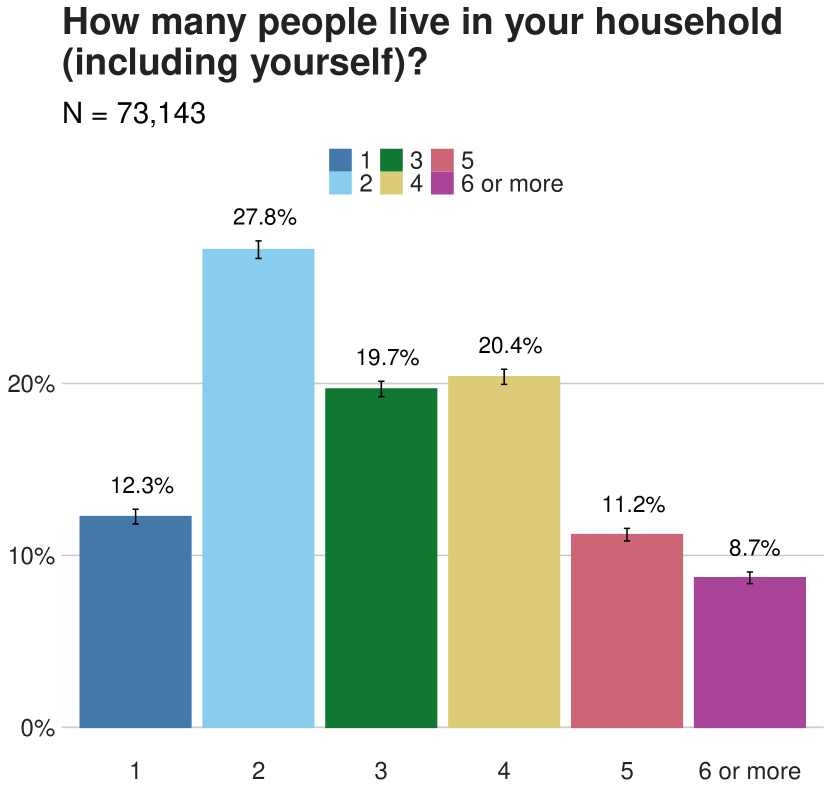
(a) Household Size Overall

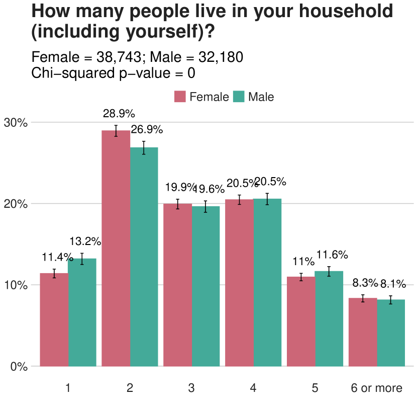
(b) Household Size by Gender

Figure 42: How many people live in your household (including yourself)?

Household Child Count - How many children 18 years or younger live in your household?

Response	Overall	Female	Male
0	42914	21908	19753
1	12010	6780	4931
2	10701	6127	4308
3	4424	2469	1845
4	1653	903	673
5 or more	1453	574	569

Table 54: Household Child Count: Weighted N, Overall and by Gender

Response	Overall	Female	Male
0	58.7 (58.1, 59.2)	56.5 (55.8, 57.3)	61.6 (60.7, 62.5)
1	16.4 (16.0, 16.8)	17.5 (16.9, 18.1)	15.4 (14.7, 16.0)
2	14.6 (14.2, 15.0)	15.8 (15.3, 16.3)	13.4 (12.8, 14.0)
3	6.0 ( 5.8, 6.3)	6.4 ( 6.0, 6.7)	5.8 ( 5.3, 6.2)
4	2.3 ( 2.1, 2.4)	2.3 ( 2.1, 2.6)	2.1 ( 1.8, 2.4)
5 or more	2.0 ( 1.8, 2.2)	1.5 ( 1.3, 1.7)	1.8 ( 1.5, 2.0)

Table 55: Household Child Count: Percent, Overall and by Gender

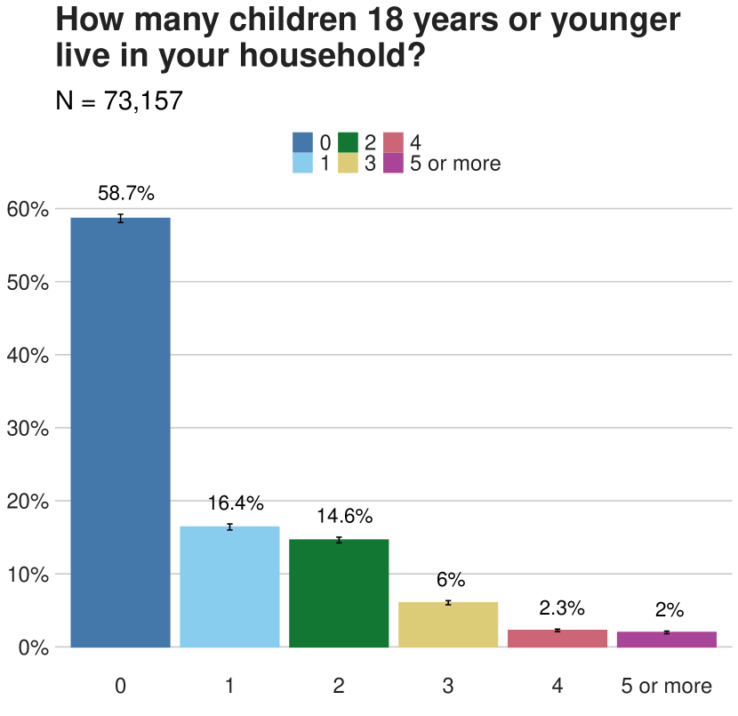
(a) Household Child Count Overall

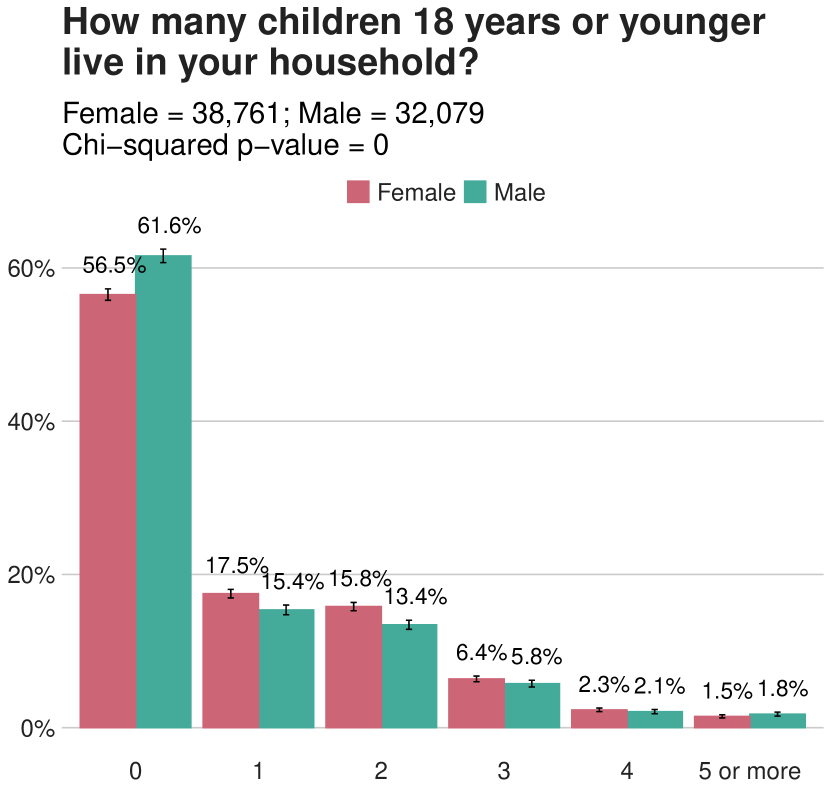
(b) Household Child Count by Gender

Figure 43: How many children 18 years or younger live in your household?

Household Partner - Do you have a spouse or long-term partner?

Response	Overall	Female	Male
Yes	37940	20615	16658
No	26162	13643	11975
Prefer not to say	7163	3507	2586

Table 56: Household Partner: Weighted N, Overall and by Gender

Response	Overall	Female	Male
Yes	53.2 (52.6, 53.8)	54.6 (53.8, 55.4)	53.4 (52.4, 54.3)
No	36.7 (36.1, 37.3)	36.1 (35.4, 36.9)	38.4 (37.4, 39.3)
Prefer not to say	10.1 ( 9.7, 10.4)	9.3 ( 8.8, 9.8)	8.3 ( 7.7, 8.8)

Table 57: Household Partner: Percent, Overall and by Gender

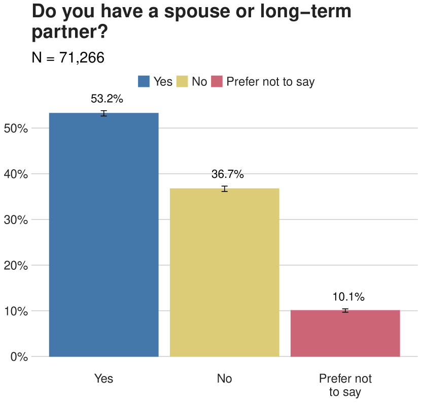
(a) Household Partner Overall

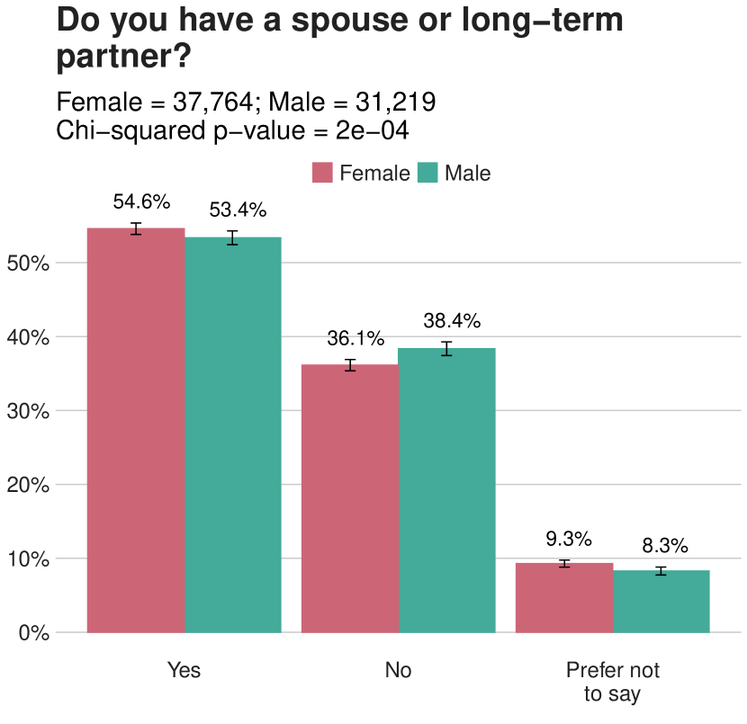
(b) Household Partner by Gender

Figure 44: Do you have a spouse or long-term partner?

Household Split Return - Did you return to your home at least one day before other members of your household?

Response	Overall	Female	Male
Yes	323	110	182
No	664	371	260
Prefer not to say	49	19	19

Table 58: Household Split Return: Weighted N, Overall and by Gender

Response	Overall	Female	Male
Yes	31.2 (26.5, 35.8)	22.0 (16.2, 27.8)	39.5 (32.0, 46.9)
No	64.1 (59.3, 68.8)	74.3 (68.3, 80.3)	56.4 (48.9, 63.9)
Prefer not to say	4.7 ( 3.3, 6.2)	3.7 ( 1.9, 5.6)	4.1 ( 2.0, 6.2)

Table 59: Household Split Return: Percent, Overall and by Gender

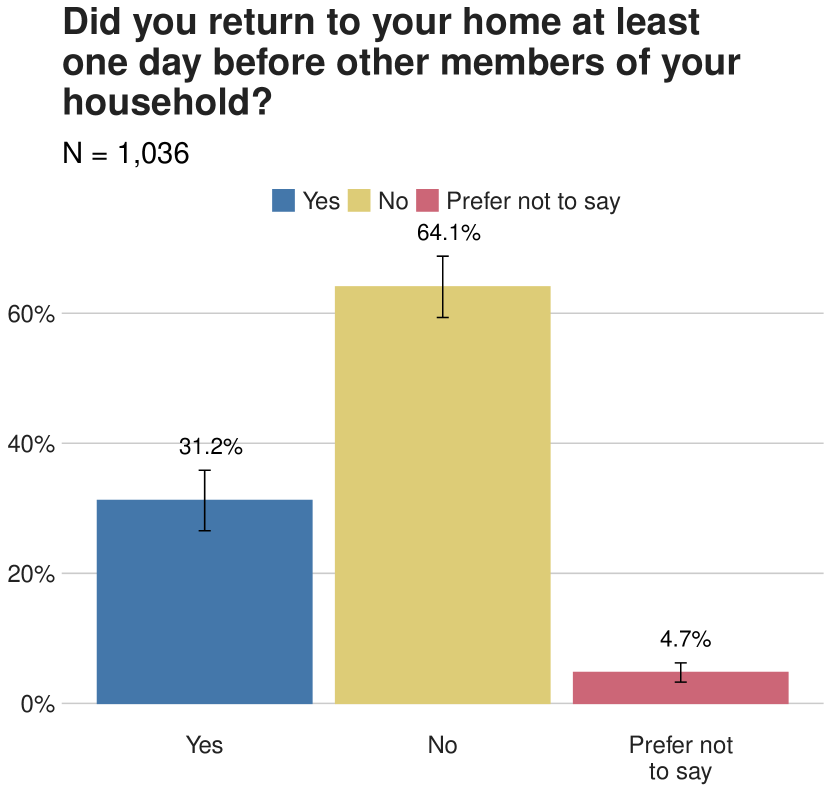
(a) Household Split Return Overall

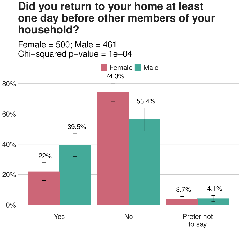
(b) Household Split Return by Gender

Figure 45: Did you return to your home at least one day before other members of your household?

Household Left Behind - When you were displaced for more than 3 nights did anyone in your household stay behind?

Response	Overall	Female	Male
Yes	252	95	98
No	646	244	253

Table 60: Household Left Behind: Weighted N, Overall and by Gender

Response	Overall	Female	Male
Yes	28.0 (23.4, 32.6)	28.1 (20.5, 35.8)	27.9 (19.9, 35.8)
No	72.0 (67.4, 76.6)	71.9 (64.2, 79.5)	72.1 (64.2, 80.1)

Table 61: Household Left Behind: Percent, Overall and by Gender

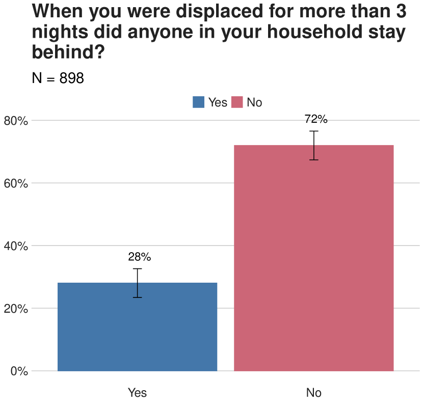
(a) Household Left Behind Overall

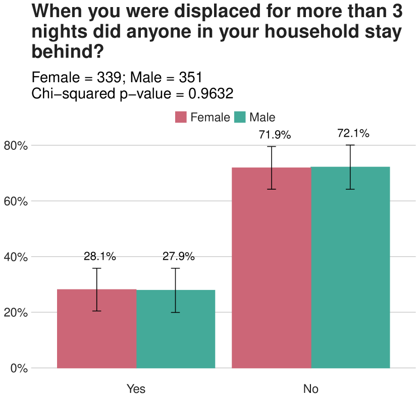
(b) Household Left Behind by Gender

Figure 46: When you were displaced for more than 3 nights did anyone in your household stay behind?

Mask Access - Do you have access to a face mask in case of excessive wildfire smoke?

Response	Overall	Female	Male
Yes	19261	9174	9431
No	42320	23356	17708

Table 62: Mask Access: Weighted N, Overall and by Gender

Response	Overall	Female	Male
Yes	31.3 (30.7, 31.9)	28.2 (27.5, 28.9)	34.8 (33.8, 35.7)
No	68.7 (68.1, 69.3)	71.8 (71.1, 72.5)	65.2 (64.3, 66.2)

Table 63: Mask Access: Percent, Overall and by Gender

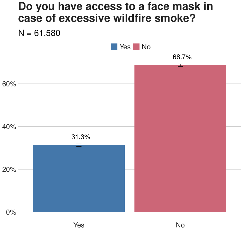
(a) Mask Access Overall

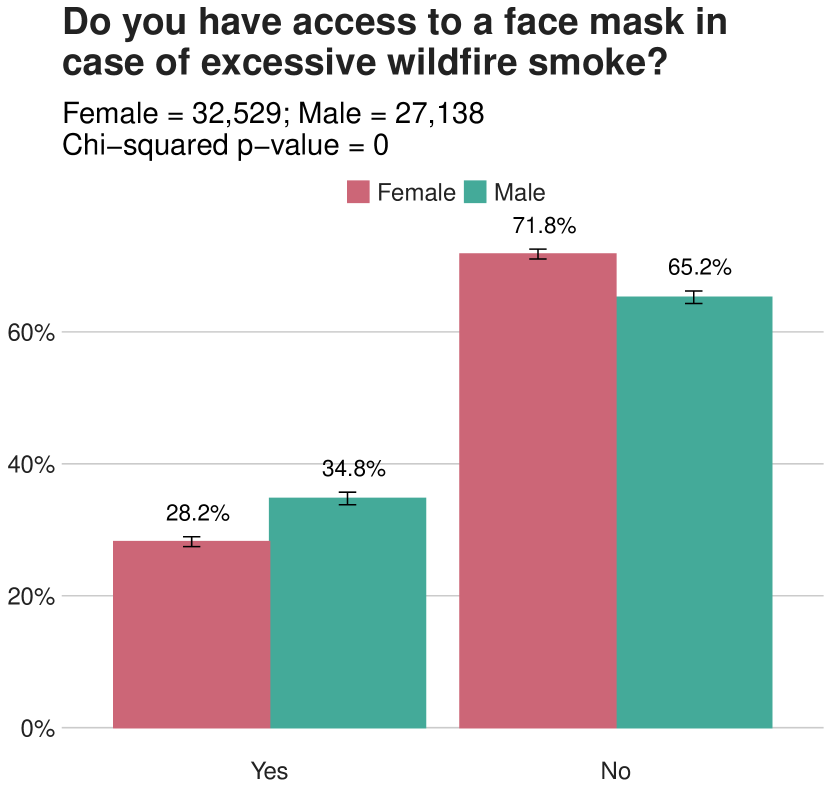
(b) Mask Access by Gender

Figure 47: Do you have access to a face mask in case of excessive wildfire smoke?

Mask Knowledge - Do you know how to tell if a face mask is effective against wildfire smoke?

Response	Overall	Female	Male
Yes	23209	10423	11978
No	37944	21926	14930

Table 64: Mask Knowledge: Weighted N, Overall and by Gender

Response	Overall	Female	Male
Yes	38.0 (37.3, 38.6)	32.2 (31.5, 33.0)	44.5 (43.5, 45.5)
No	62.0 (61.4, 62.7)	67.8 (67.0, 68.5)	55.5 (54.5, 56.5)

Table 65: Mask Knowledge: Percent, Overall and by Gender

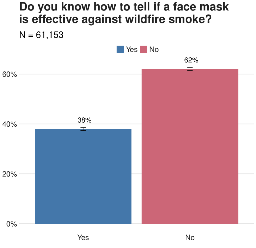
(a) Mask Knowledge Overall

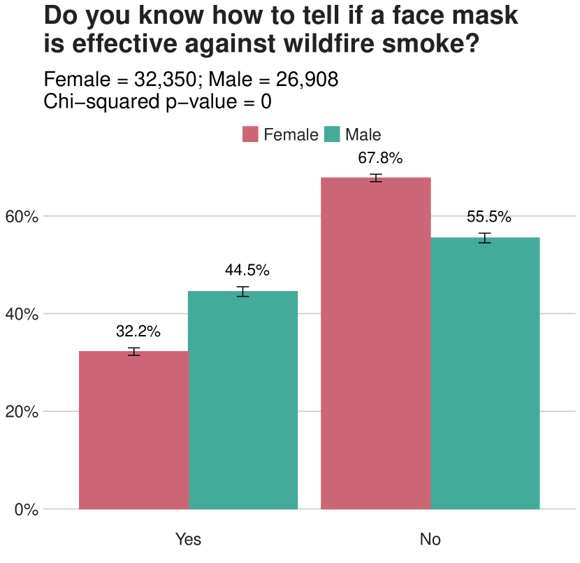
(b) Mask Knowledge by Gender

Figure 48: Do you know how to tell if a face mask is effective against wildfire smoke?

On Vacation - Were you on holiday in this area on December 18, 2019?

Response	Overall	Female	Male
Yes	3179	1130	1503
No	15636	7249	6705

Table 66: On Vacation: Weighted N, Overall and by Gender

Response	Overall	Female	Male
Yes	16.9 (16.0, 17.8)	13.5 (12.3, 14.7)	18.3 (16.8, 19.9)
No	83.1 (82.2, 84.0)	86.5 (85.3, 87.7)	81.7 (80.1, 83.2)

Table 67: On Vacation: Percent, Overall and by Gender

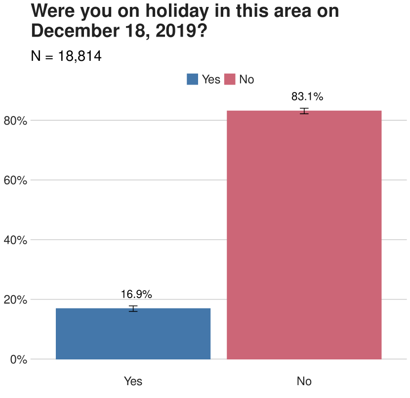
(a) On Vacation Overall

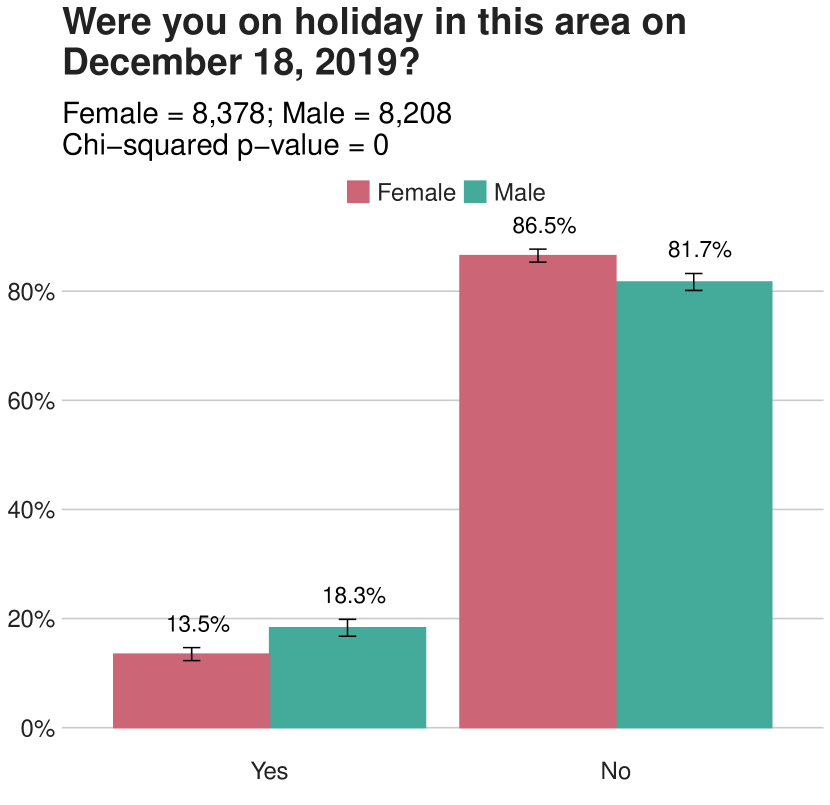
(b) On Vacation by Gender

Figure 49: Were you on holiday in this area on December 18, 2019?

Travel Check - Did you go on holiday or work travel away from your home for more than one night between Dec. 18, 2019 and Jan. 1, 2020?

Response	Overall	Female	Male
Yes	26695	12845	12453
No	53794	28108	21923
I don’t know	1623	454	570

Table 68: Travel Check: Weighted N, Overall and by Gender

Response	Overall	Female	Male
Yes	32.5 (32.0, 33.0)	31.0 (30.3, 31.7)	35.6 (34.8, 36.5)
No	65.5 (65.0, 66.0)	67.9 (67.2, 68.6)	62.7 (61.9, 63.6)
I don’t know	2.0 ( 1.8, 2.2)	1.1 ( 0.9, 1.3)	1.6 ( 1.4, 1.9)

Table 69: Travel Check: Percent, Overall and by Gender

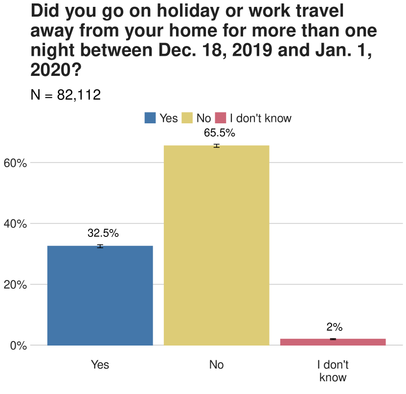
(a) Travel Check Overall

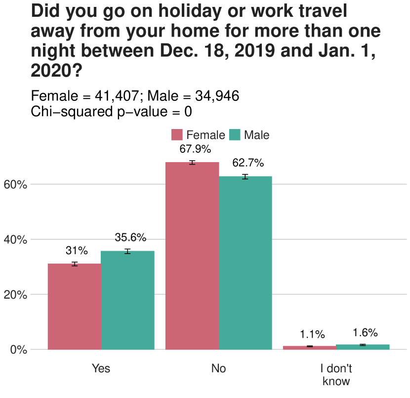
(b) Travel Check by Gender

Figure 50: Did you go on holiday or work travel away from your home for more than one night between Dec. 18, 2019 and Jan. 1, 2020?

In Area Gatekeeper - Have you been in an area directly affected by the Australian bushfires that began on December 18, 2019?

Response	Overall	Female	Male
Yes	26579	8629	8462
No	66084	32317	26175
I don’t know	2867	1184	977

Table 70: In Area Gatekeeper: Weighted N, Overall and by Gender

Response	Overall	Female	Male
Yes	27.8 (27.4, 28.3)	20.5 (19.9, 21.1)	23.8 (23.0, 24.5)
No	69.2 (68.7, 69.7)	76.7 (76.1, 77.3)	73.5 (72.7, 74.3)
I don’t know	3.0 ( 2.8, 3.2)	2.8 ( 2.5, 3.1)	2.7 ( 2.4, 3.1)

Table 71: In Area Gatekeeper: Percent, Overall and by Gender

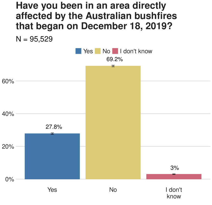
(a) In Area Gatekeeper Overall

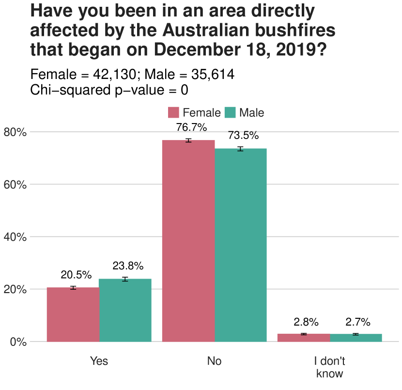
(b) In Area Gatekeeper by Gender

Figure 51: Have you been in an area directly affected by the Australian bushfires that began on December 18, 2019?

Appendix 2

Supplementary Regression Models

This section includes extra regression models we ran in the course of analyzing the survey. Each subsection presents one model, first as a plot followed by the corresponding table. Captions describe the model and the reference group for the odds ratios.

Evacuation Decision Regression: Model with Age and Gender Interaction Effects

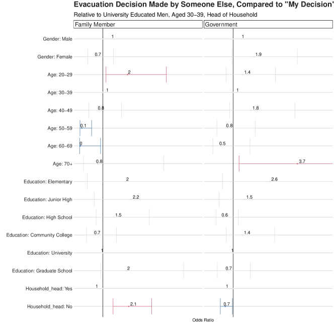
Figure 52: Evacuation decision made by someone else, compared to “my decision”; relative to university educated men, aged 30-39, head of household based on model with age and gender interactions, and education and head of household main effects

Table 72: Evacuation decision made by someone else, compared to “my decision”; relative to university educated men, aged 30-39, head of household based on model with age and gender interactions, and education and head of household main effects

Response	Covariate	Odds Ratio	95% CI	P Value	Significance
Family Member	Gender: Male	1.00
Family Member	Gender: Female	0.72	(0.36, 1.4)	0.357
Family Member	Age: 20-29	2.05	(1.13, 3.7)	0.018	*
Family Member	Age: 30-39	1.00
Family Member	Age: 40-49	0.84	(0.40, 1.8)	0.658
Family Member	Age: 50-59	0.10	(0.02, 0.5)	0.006	**
Family Member	Age: 60-69	0.03	(0.00, 0.9)	0.043	*
Family Member	Age: 70+	0.78	(0.17, 3.6)	0.746
Family Member	Education: Elementary	1.97	(0.33, 11.8)	0.459
Family Member	Education: Junior High	2.21	(0.62, 7.8)	0.219
Family Member	Education: High School	1.45	(0.71, 3.0)	0.306
Family Member	Education: Community College	0.69	(0.30, 1.6)	0.378
Family Member	Education: University	1.00
Family Member	Education: Graduate School	2.01	(0.91, 4.4)	0.086	.
Family Member	Household_head: Yes	1.00
Family Member	Household_head: No	2.10	(1.43, 3.1)	0.000	***
Government	Gender: Male	1.00
Government	Gender: Female	1.88	(0.94, 3.7)	0.073	.
Government	Age: 20-29	1.40	(0.70, 2.8)	0.337
Government	Age: 30-39	1.00
Government	Age: 40-49	1.76	(0.85, 3.6)	0.126
Government	Age: 50-59	0.77	(0.31, 1.9)	0.581
Government	Age: 60-69	0.48	(0.13, 1.7)	0.259
Government	Age: 70+	3.74	(1.25, 11.2)	0.018	*
Government	Education: Elementary	2.57	(0.54, 12.1)	0.234
Government	Education: Junior High	1.49	(0.40, 5.5)	0.555
Government	Education: High School	0.57	(0.27, 1.2)	0.149
Government	Education: Community College	1.40	(0.71, 2.8)	0.338
Government	Education: University	1.00
Government	Education: Graduate School	0.75	(0.32, 1.7)	0.497
Government	Household_head: Yes	1.00
Government	Household_head: No	0.66	(0.45, 1.0)	0.033	*

Household Split Return Regression: Model With No Interactions

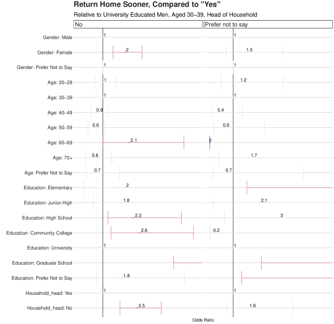
Figure 53: Return home sooner, compared to “yes”; relative to university educated men, aged 30-39, head of household based on model with main effects for age, gender, education, and head of household with no interactions

Table 73: Return home sooner, compared to “yes”; relative to university educated men, aged 30-39, head of household based on model with main effects for age, gender, education, and head of household with no interactions

Response	Covariate	Odds Ratio	95% CI	P Value	Significance
No	Gender: Male	1.00
No	Gender: Female	1.96	(1.43, 2.7)	0.000	***
No	Gender: Prefer Not to Say	1.00	(1.00, 1.0)	1.000
No	Age: 20-29	1.01	(0.66, 1.6)	0.953
No	Age: 30-39	1.00
No	Age: 40-49	0.79	(0.51, 1.2)	0.295
No	Age: 50-59	0.62	(0.36, 1.1)	0.080	.
No	Age: 60-69	2.12	(1.00, 4.5)	0.049	*
No	Age: 70+	0.60	(0.26, 1.4)	0.215
No	Age: Prefer Not to Say	0.69	(0.28, 1.7)	0.425
No	Education: Elementary	1.97	(0.18, 22.0)	0.581
No	Education: Junior High	1.80	(0.58, 5.5)	0.307
No	Education: High School	2.30	(1.22, 4.4)	0.010	*
No	Education: Community College	2.56	(1.35, 4.9)	0.004	**
No	Education: University	1.00
No	Education: Graduate School	10.14	(4.02, 25.6)	0.000	***
No	Education: Prefer Not to Say	1.80	(0.73, 4.5)	0.204
No	Household_head: Yes	1.00
No	Household_head: No	2.45	(1.73, 3.5)	0.000	***
Prefer not to say	Gender: Male	1.00
Prefer not to say	Gender: Female	1.49	(0.71, 3.1)	0.290
Prefer not to say	Gender: Prefer Not to Say	1.00	(1.00, 1.0)	1.000
Prefer not to say	Age: 20-29	1.23	(0.48, 3.1)	0.663
Prefer not to say	Age: 30-39	1.00
Prefer not to say	Age: 40-49	0.40	(0.11, 1.4)	0.149
Prefer not to say	Age: 50-59	0.63	(0.17, 2.4)	0.494
Prefer not to say	Age: 60-69	0.00	(0.00, 0.0)	0.000	***
Prefer not to say	Age: 70+	1.69	(0.39, 7.3)	0.487
Prefer not to say	Age: Prefer Not to Say	0.74	(0.14, 4.0)	0.730
Prefer not to say	Education: Elementary	30.15	(1.59, 571.8)	0.023	*
Prefer not to say	Education: Junior High	2.13	(0.15, 30.1)	0.577
Prefer not to say	Education: High School	2.99	(0.64, 14.0)	0.165
Prefer not to say	Education: Community College	0.22	(0.01, 6.5)	0.379
Prefer not to say	Education: University	1.00
Prefer not to say	Education: Graduate School	12.32	(2.20, 69.0)	0.004	**
Prefer not to say	Education: Prefer Not to Say	7.55	(1.37, 41.7)	0.020	*
Prefer not to say	Household_head: Yes	1.00
Prefer not to say	Household_head: No	1.63	(0.75, 3.5)	0.222

Mask Knowledge Regression: Model With No Interactions

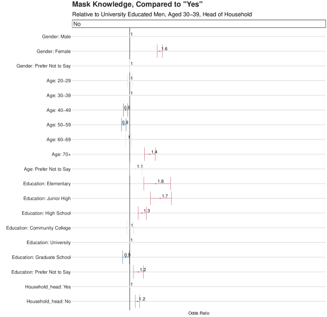
Figure 54: Mask knowledge, compared to “yes”; relative to university educated men, aged 30-39, head of household based on model with main effects for age, gender, education, and head of household with no interactions

Table 74: Mask knowledge, compared to “yes”; relative to university educated men, aged 30-39, head of household based on model with main effects for age, gender, education, and head of household with no interactions

Response	Covariate	Odds Ratio	95% CI	P Value	Significance
No	Gender: Male	1.00
No	Gender: Female	1.65	(1.59, 1.7)	0.000	***
No	Gender: Prefer Not to Say	1.00	(1.00, 1.0)	1.000
No	Age: 20-29	1.00	(0.95, 1.1)	0.968
No	Age: 30-39	1.00
No	Age: 40-49	0.91	(0.86, 1.0)	0.000	***
No	Age: 50-59	0.87	(0.82, 0.9)	0.000	***
No	Age: 60-69	0.97	(0.91, 1.0)	0.348
No	Age: 70+	1.43	(1.32, 1.6)	0.000	***
No	Age: Prefer Not to Say	1.12	(1.00, 1.3)	0.059	.
No	Education: Elementary	1.57	(1.30, 1.9)	0.000	***
No	Education: Junior High	1.66	(1.45, 1.9)	0.000	***
No	Education: High School	1.27	(1.18, 1.4)	0.000	***
No	Education: Community College	1.01	(0.94, 1.1)	0.800
No	Education: University	1.00
No	Education: Graduate School	0.92	(0.84, 1.0)	0.032	*
No	Education: Prefer Not to Say	1.18	(1.08, 1.3)	0.000	***
No	Household_head: Yes	1.00
No	Household_head: No	1.17	(1.12, 1.2)	0.000	***

More than One Night Regression: Model With No Interactions

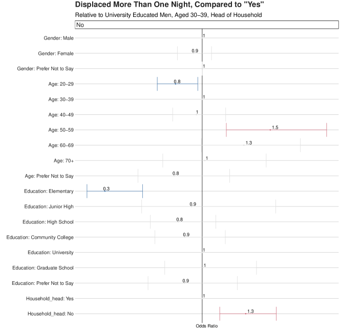
Figure 55: Not displaced more than one night, compared to “yes”; relative to university educated men, aged 30-39, head of household based on model with main effects for age, gender, education, and head of household with no interactions

Table 75: Displaced more than one night, compared to “yes”; relative to university educated men, aged 30-39, head of household based on model with main effects for age, gender, education, and head of household with no interactions

Response	Covariate	Odds Ratio	95% CI	P Value	Significance
No	Gender: Male	1.00
No	Gender: Female	0.93	(0.81, 1.1)	0.320
No	Gender: Prefer Not to Say	1.00	(1.00, 1.0)	1.000
No	Age: 20-29	0.80	(0.66, 1.0)	0.021	*
No	Age: 30-39	1.00
No	Age: 40-49	0.96	(0.78, 1.2)	0.673
No	Age: 50-59	1.52	(1.18, 1.9)	0.001	**
No	Age: 60-69	1.32	(0.99, 1.7)	0.056	.
No	Age: 70+	1.02	(0.70, 1.5)	0.917
No	Age: Prefer Not to Say	0.79	(0.51, 1.2)	0.273
No	Education: Elementary	0.26	(0.12, 0.5)	0.000	***
No	Education: Junior High	0.92	(0.54, 1.6)	0.751
No	Education: High School	0.82	(0.60, 1.1)	0.187
No	Education: Community College	0.87	(0.64, 1.2)	0.359
No	Education: University	1.00
No	Education: Graduate School	1.01	(0.71, 1.4)	0.976
No	Education: Prefer Not to Say	0.86	(0.59, 1.3)	0.452
No	Household_head: Yes	1.00
No	Household_head: No	1.33	(1.13, 1.6)	0.000	***

Mask Knowledge Regression: Model with Mask Access, No Interactions

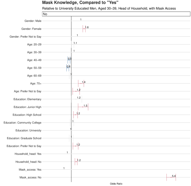
Figure 56: Mask knowledge, compared to “yes”; relative to university educated men, aged 30-39, head of household, with mask access based on model with main effects for age, gender, education, and head of household with no interactions

Table 76: Mask knowledge, compared to “yes”; relative to university educated men, aged 30-39, head of household, with mask access based on model with main effects for age, gender, education, and head of household with no interactions

Response	Covariate	Odds Ratio	95% CI	P Value	Significance
No	Gender: Male	1.00
No	Gender: Female	1.57	(1.51, 1.6)	0.000	***
No	Gender: Prefer Not to Say	1.00	(NaN, NaN)	NaN
No	Age: 20-29	1.06	(1.00, 1.1)	0.057	.
No	Age: 30-39	1.00
No	Age: 40-49	0.89	(0.84, 0.9)	0.000	***
No	Age: 50-59	0.84	(0.79, 0.9)	0.000	***
No	Age: 60-69	0.97	(0.91, 1.0)	0.464
No	Age: 70+	1.43	(1.31, 1.6)	0.000	***
No	Age: Prefer Not to Say	1.21	(1.06, 1.4)	0.004	**
No	Education: Elementary	1.21	(1.00, 1.5)	0.056	.
No	Education: Junior High	1.51	(1.30, 1.7)	0.000	***
No	Education: High School	1.19	(1.10, 1.3)	0.000	***
No	Education: Community College	1.02	(0.95, 1.1)	0.550
No	Education: University	1.00
No	Education: Graduate School	0.99	(0.90, 1.1)	0.764
No	Education: Prefer Not to Say	1.18	(1.07, 1.3)	0.001	***
No	Household_head: Yes	1.00
No	Household_head: No	1.21	(1.16, 1.3)	0.000	***
No	Mask_access: Yes	1.00
No	Mask_access: No	5.45	(5.24, 5.7)	0.000	***

Mask Access Regression: Model With Income Displacement, No Interactions

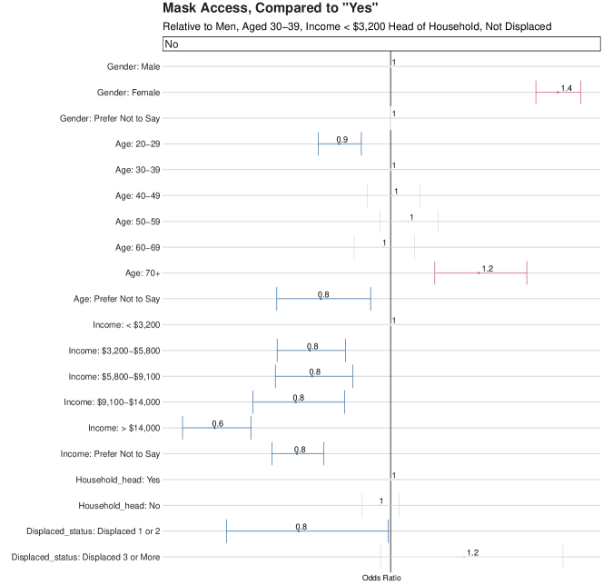
Figure 57: Mask access, compared to “yes”; relative to men, aged 30-39, income less than $3,200 head of household, not displaced based on model with main effects for age, gender, income, head of household, and duration displaced with no interactions

Table 77: Mask access, compared to “yes”; relative to men, aged 30-39, income less than $3,200 head of household, not displaced based on model with main effects for age, gender, income, head of household, and duration displaced with no interactions

Response	Covariate	Odds Ratio	95% CI	P Value	Significance
No	Gender: Male	1.00
No	Gender: Female	1.36	(1.32, 1.4)	0.000	***
No	Gender: Prefer Not to Say	1.00	(1.00, 1.0)	1.000
No	Age: 20-29	0.89	(0.84, 0.9)	0.000	***
No	Age: 30-39	1.00
No	Age: 40-49	1.00	(0.95, 1.1)	0.875
No	Age: 50-59	1.04	(0.98, 1.1)	0.227
No	Age: 60-69	0.98	(0.92, 1.1)	0.641
No	Age: 70+	1.19	(1.10, 1.3)	0.000	***
No	Age: Prefer Not to Say	0.85	(0.75, 1.0)	0.007	**
No	Income: $<$ $3,200	1.00
No	Income: $3,200-$5,800	0.82	(0.75, 0.9)	0.000	***
No	Income: $5,800-$9,100	0.83	(0.75, 0.9)	0.000	***
No	Income: $9,100-$14,000	0.79	(0.70, 0.9)	0.000	***
No	Income: $>$ $14,000	0.62	(0.55, 0.7)	0.000	***
No	Income: Prefer Not to Say	0.80	(0.74, 0.9)	0.000	***
No	Household_head: Yes	1.00
No	Household_head: No	0.98	(0.94, 1.0)	0.279
No	Displaced_status: Displaced 1-3 nights	0.80	(0.64, 1.0)	0.045	*
No	Displaced_status: Displaced more than 3 nights	1.16	(0.98, 1.4)	0.088	.

Household Split Return Regression: Model With Child Count, No Interactions

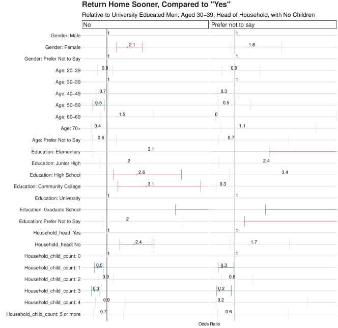
Figure 58: Return home sooner, compared to “yes”; relative to university educated men, aged 30-39, head of household, with no children based on model with main effects for age, gender, education, and head of household with no interactions

Table 78: Return home sooner, compared to “yes”; relative to university educated men, aged 30-39, head of household, with no children based on model with main effects for age, gender, education, and head of household with no interactions

Response	Covariate	Odds Ratio	95% CI	P Value	Significance
No	Gender: Male	1.00
No	Gender: Female	2.07	(1.51, 2.9)	0.000	***
No	Gender: Prefer Not to Say	1.00	(NaN, NaN)	NaN
No	Age: 20-29	0.81	(0.51, 1.3)	0.382
No	Age: 30-39	1.00
No	Age: 40-49	0.69	(0.44, 1.1)	0.120
No	Age: 50-59	0.48	(0.27, 0.9)	0.014	*
No	Age: 60-69	1.54	(0.69, 3.5)	0.294
No	Age: 70+	0.44	(0.19, 1.0)	0.059	.
No	Age: Prefer Not to Say	0.60	(0.24, 1.5)	0.274
No	Education: Elementary	3.06	(0.27, 34.5)	0.366
No	Education: Junior High	2.04	(0.63, 6.6)	0.236
No	Education: High School	2.57	(1.35, 4.9)	0.004	**
No	Education: Community College	3.05	(1.58, 5.9)	0.001	***
No	Education: University	1.00
No	Education: Graduate School	11.68	(4.57, 29.8)	0.000	***
No	Education: Prefer Not to Say	1.98	(0.79, 5.0)	0.146
No	Household_head: Yes	1.00
No	Household_head: No	2.41	(1.68, 3.5)	0.000	***
No	Household_child_count: 0	1.00
No	Household_child_count: 1	0.52	(0.34, 0.8)	0.003	**
No	Household_child_count: 2	0.86	(0.55, 1.3)	0.515
No	Household_child_count: 3	0.35	(0.20, 0.6)	0.000	***
No	Household_child_count: 4	0.89	(0.41, 2.0)	0.775
No	Household_child_count: 5 or more	0.74	(0.29, 1.9)	0.518
Prefer not to say	Gender: Male	1.00
Prefer not to say	Gender: Female	1.63	(0.77, 3.4)	0.198
Prefer not to say	Gender: Prefer Not to Say	1.00	(1.00, 1.0)	1.000
Prefer not to say	Age: 20-29	0.86	(0.32, 2.3)	0.770
Prefer not to say	Age: 30-39	1.00
Prefer not to say	Age: 40-49	0.34	(0.10, 1.2)	0.095	.
Prefer not to say	Age: 50-59	0.46	(0.12, 1.8)	0.269
Prefer not to say	Age: 60-69	0.00	(0.00, Inf)	0.972
Prefer not to say	Age: 70+	1.13	(0.25, 5.2)	0.873
Prefer not to say	Age: Prefer Not to Say	0.72	(0.13, 3.8)	0.695
Prefer not to say	Education: Elementary	61.01	(2.78, 1338.4)	0.009	**
Prefer not to say	Education: Junior High	2.39	(0.16, 36.1)	0.528
Prefer not to say	Education: High School	3.36	(0.70, 16.1)	0.129
Prefer not to say	Education: Community College	0.28	(0.01, 8.6)	0.466
Prefer not to say	Education: University	1.00
Prefer not to say	Education: Graduate School	14.84	(2.59, 85.1)	0.002	**
Prefer not to say	Education: Prefer Not to Say	8.41	(1.50, 47.3)	0.016	*
Prefer not to say	Household_head: Yes	1.00
Prefer not to say	Household_head: No	1.73	(0.78, 3.8)	0.175
Prefer not to say	Household_child_count: 0	1.00
Prefer not to say	Household_child_count: 1	0.34	(0.12, 0.9)	0.039	*
Prefer not to say	Household_child_count: 2	0.77	(0.31, 1.9)	0.584
Prefer not to say	Household_child_count: 3	0.20	(0.05, 0.8)	0.023	*
Prefer not to say	Household_child_count: 4	0.18	(0.01, 4.8)	0.302
Prefer not to say	Household_child_count: 5 or more	0.59	(0.09, 3.8)	0.580

Prevent Working Regression: Model With Education, No Interactions

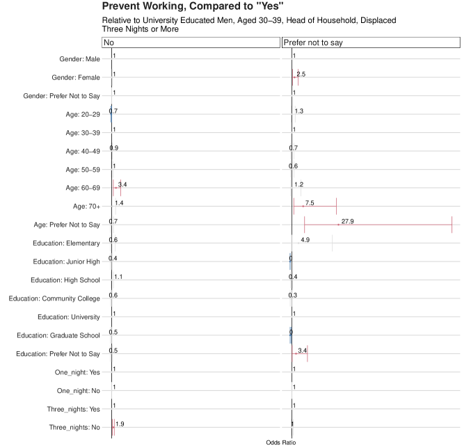
Figure 59: Prevent working, compared to “yes”; relative to university educated men, aged 30-39, head of household, displaced more than three nights based on model with main effects for age, gender, education, and head of household with no interactions

Table 79: Prevent working, compared to “yes”; relative to university educated men, aged 30-39, head of household, displaced more than three nights based on model with main effects for age, gender, education, and head of household with no interactions

Response	Covariate	Odds Ratio	95% CI	P Value	Significance
No	Gender: Male	1.00
No	Gender: Female	1.04	(0.79, 1.4)	0.783
No	Gender: Prefer Not to Say	1.00	(1.00, 1.0)	1.000
No	Age: 20-29	0.67	(0.45, 1.0)	0.038	*
No	Age: 30-39	1.00
No	Age: 40-49	0.93	(0.62, 1.4)	0.730
No	Age: 50-59	1.03	(0.62, 1.7)	0.919
No	Age: 60-69	3.44	(1.90, 6.2)	0.000	***
No	Age: 70+	1.45	(0.65, 3.2)	0.363
No	Age: Prefer Not to Say	0.67	(0.22, 2.0)	0.477
No	Education: Elementary	0.62	(0.13, 3.0)	0.545
No	Education: Junior High	0.41	(0.15, 1.1)	0.089	.
No	Education: High School	1.09	(0.61, 1.9)	0.762
No	Education: Community College	0.61	(0.34, 1.1)	0.105
No	Education: University	1.00
No	Education: Graduate School	0.54	(0.28, 1.1)	0.072	.
No	Education: Prefer Not to Say	0.52	(0.22, 1.2)	0.137
No	More than One night: Yes	1.00
No	More than One night: No	1.00	(1.00, 1.0)	1.000
No	More than Three Nights: Yes	1.00
No	More than Three Nights: No	1.86	(1.40, 2.5)	0.000	***
Prefer not to say	Gender: Male	1.00
Prefer not to say	Gender: Female	2.55	(1.40, 4.6)	0.002	**
Prefer not to say	Gender: Prefer Not to Say	1.00	(NaN, NaN)	NaN
Prefer not to say	Age: 20-29	1.27	(0.55, 2.9)	0.576
Prefer not to say	Age: 30-39	1.00
Prefer not to say	Age: 40-49	0.71	(0.24, 2.1)	0.541
Prefer not to say	Age: 50-59	0.57	(0.14, 2.2)	0.417
Prefer not to say	Age: 60-69	1.25	(0.25, 6.2)	0.786
Prefer not to say	Age: 70+	7.54	(2.13, 26.7)	0.002	**
Prefer not to say	Age: Prefer Not to Say	27.94	(8.35, 93.5)	0.000	***
Prefer not to say	Education: Elementary	4.88	(0.98, 24.3)	0.053	.
Prefer not to say	Education: Junior High	0.00	(0.00, 0.0)	0.000	***
Prefer not to say	Education: High School	0.45	(0.15, 1.3)	0.147
Prefer not to say	Education: Community College	0.26	(0.07, 1.0)	0.055	.
Prefer not to say	Education: University	1.00
Prefer not to say	Education: Graduate School	0.03	(0.00, 0.7)	0.030	*
Prefer not to say	Education: Prefer Not to Say	3.41	(1.16, 10.0)	0.025	*
Prefer not to say	More than One night: Yes	1.00
Prefer not to say	More than One night: No	1.00	(1.00, 1.0)	NaN
Prefer not to say	More than Three nights: Yes	1.00
Prefer not to say	More than Three nights: No	0.97	(0.54, 1.7)	0.920

References

- Alexander et al (2019) Alexander M, Zagheni E, Polimis K (2019) The impact of hurricane maria on out-migration from puerto rico: Evidence from facebook data
- Belasen and Polachek (2013) Belasen AR, Polachek SW (2013) Natural disasters and migration. In: international Handbook on the Economics of migration, Edward Elgar Publishing
- Blondel et al (2015) Blondel VD, Decuyper A, Krings G (2015) A survey of results on mobile phone datasets analysis. EPJ data science 4(1):10
- Bouwer (2011) Bouwer LM (2011) Have disaster losses increased due to anthropogenic climate change? Bulletin of the American Meteorological Society 92(1):39–46
- Czajkowski and Kennedy (2010) Czajkowski J, Kennedy E (2010) Fatal tradeoff? toward a better understanding of the costs of not evacuating from a hurricane in landfall counties. Population and environment 31(1-3):121–149
- Davies and Hemmeter (2010) Davies PS, Hemmeter J (2010) Supplemental security income recipients affected by hurricanes katrina and rita: an analysis of two years of administrative data. Population and Environment 31(1-3):87–120
- Deville et al (2014) Deville P, Linard C, Martin S, Gilbert M, Stevens FR, Gaughan AE, Blondel VD, Tatem AJ (2014) Dynamic population mapping using mobile phone data. Proceedings of the National Academy of Sciences 111(45):15888–15893
- Donner and Rodríguez (2008) Donner W, Rodríguez H (2008) Population composition, migration and inequality: The influence of demographic changes on disaster risk and vulnerability. Social forces 87(2):1089–1114
- Dynes et al (1987) Dynes RR, De Marchi B, Pelanda C (1987) Sociology of disasters. Milano: Franco Angelli
- Feehan and Cobb (2019) Feehan DM, Cobb C (2019) Using an online sample to estimate the size of an offline population. Demography 56(6):2377–2392
- Filkov et al (2020) Filkov AI, Ngo T, Matthews S, Telfer S, Penman TD (2020) Impact of australia’s catastrophic 2019/20 bushfire season on communities and environment. retrospective analysis and current trends. Journal of Safety Science and Resilience
- Finlay (2009) Finlay JE (2009) Fertility response to natural disasters: the case of three high mortality earthquakes. The World Bank
- Frankenberg et al (2013) Frankenberg E, Friedman J, Ingwerson N, Thomas D (2013) Child height after a natural disaster. Duke University
- Frankenberg et al (2014) Frankenberg E, Laurito M, Thomas D (2014) The demography of disasters. Prepared for the International Encyclopedia of the Social and Behavioral Sciences 2nd ed(Area) 3:12
- Frey and Singer (2010) Frey WH, Singer A (2010) Demographic dynamics and natural disasters: learning from katrina and rita
- Fussell et al (2010) Fussell E, Sastry N, VanLandingham M (2010) Race, socioeconomic status, and return migration to new orleans after hurricane katrina. Population and environment 31(1-3):20–42
- Gething and Tatem (2011) Gething PW, Tatem AJ (2011) Can mobile phone data improve emergency response to natural disasters? PLoS Med 8(8):e1001085
- Gilks and Wild (1992) Gilks WR, Wild P (1992) Adaptive rejection sampling for gibbs sampling. Journal of the Royal Statistical Society: Series C (Applied Statistics) 41(2):337–348
- Gray et al (2014) Gray C, Frankenberg E, Gillespie T, Sumantri C, Thomas D (2014) Studying displacement after a disaster using large-scale survey methods: Sumatra after the 2004 tsunami. Annals of the Association of American Geographers 104(3):594–612
- Groves and Lyberg (2010) Groves RM, Lyberg L (2010) Total survey error: Past, present, and future. Public opinion quarterly 74(5):849–879
- Gutmann and Field (2010) Gutmann MP, Field V (2010) Katrina in historical context: environment and migration in the us. Population and environment 31(1-3):3–19
- Hori and Schafer (2010) Hori M, Schafer MJ (2010) Social costs of displacement in louisiana after hurricanes katrina and rita. Population and environment 31(1-3):64–86
- James and Paton (2015) James H, Paton D (2015) The consequences of disasters: Demographic, planning, and policy implications. Charles C Thomas Publisher
- Kganyago and Shikwambana (2020) Kganyago M, Shikwambana L (2020) Assessment of the characteristics of recent major wildfires in the usa, australia and brazil in 2018–2019 using multi-source satellite products. Remote Sensing 12(11):1803
- Lin (2010) Lin CYC (2010) Instability, investment, disasters, and demography: natural disasters and fertility in italy (1820–1962) and japan (1671–1965). Population and environment 31(4):255–281
- Lu et al (2012) Lu X, Bengtsson L, Holme P (2012) Predictability of population displacement after the 2010 haiti earthquake. Proceedings of the National Academy of Sciences 109(29):11576–11581
- Maas et al (2019) Maas P, Iyer S, Gros A, Park W, McGorman L, Nayak C, Dow PA (2019) Facebook disaster maps: Aggregate insights for crisis response & recovery. In: ISCRAM
- Overton and Stehman (1995) Overton WS, Stehman SV (1995) The horvitz-thompson theorem as a unifying perspective for probability sampling: with examples from natural resource sampling. The American Statistician 49(3):261–268
- Plyer et al (2010) Plyer A, Bonaguro J, Hodges K (2010) Using administrative data to estimate population displacement and resettlement following a catastrophic us disaster. Population and Environment 31(1-3):150–175
- Raker (2020) Raker EJ (2020) Natural hazards, disasters, and demographic change: The case of severe tornadoes in the united states, 1980–2010. Demography pp 1–22
- Ribeiro et al (2020) Ribeiro FN, Benevenuto F, Zagheni E (2020) How biased is the population of facebook users? comparing the demographics of facebook users with census data to generate correction factors. arXiv preprint arXiv:200508065
- Schneider and Harknett (2019) Schneider D, Harknett K (2019) What’s to like? facebook as a tool for survey data collection. Sociological Methods & Research p 0049124119882477
- Schultz and Elliott (2013) Schultz J, Elliott JR (2013) Natural disasters and local demographic change in the united states. Population and Environment 34(3):293–312
- Smelser et al (2001) Smelser NJ, Baltes PB, et al (2001) International encyclopedia of the social & behavioral sciences, vol 11. Elsevier Amsterdam
- Smith and McCarty (1996) Smith SK, McCarty C (1996) Demographic effects of natural disasters: A case study of hurricane andrew. Demography 33(2):265–275
- Stewart et al (2019) Stewart I, Flores RD, Riffe T, Weber I, Zagheni E (2019) Rock, rap, or reggaeton?: Assessing mexican immigrants’ cultural assimilation using facebook data. In: The World Wide Web Conference, pp 3258–3264
- Stringfield (2010) Stringfield JD (2010) Higher ground: an exploratory analysis of characteristics affecting returning populations after hurricane katrina. Population and Environment 31(1-3):43–63
- Tatem (2017) Tatem AJ (2017) Worldpop, open data for spatial demography. Scientific data 4(1):1–4
- Thomas et al (2015) Thomas TN, Leander-Griffith M, Harp V, Cioffi JP (2015) Influences of preparedness knowledge and beliefs on household disaster preparedness. Morbidity and Mortality Weekly Report 64(35):965–971
- Zagheni et al (2017) Zagheni E, Weber I, Gummadi K (2017) Leveraging facebook’s advertising platform to monitor stocks of migrants. Population and Development Review pp 721–734