From Ji to Jaffe-Manohar orbital angular momentum in Lattice QCD using a direct derivative method

Abstract

A Lattice QCD approach to quark orbital angular momentum in the proton based on generalized transverse momentum-dependent parton distributions (GTMDs) is enhanced methodologically by incorporating a direct derivative technique. This improvement removes a significant numerical bias that had been seen to afflict results of a previous study. In particular, the value obtained for Ji quark orbital angular momentum is reconciled with the one obtained independently via Ji’s sum rule, validating the GMTD approach. Since GTMDs simultaneously contain information about the quark impact parameter and transverse momentum, they permit a direct evaluation of the cross product of the latter. They are defined through proton matrix elements of a quark bilocal operator containing a Wilson line; the choice in Wilson line path allows one to continuously interpolate from Ji to Jaffe-Manohar quark orbital angular momentum. The latter is seen to be significantly enhanced in magnitude compared to Ji quark orbital angular momentum, confirming previous results.

I Introduction

The manner in which the spin of the proton arises from the spins and orbital angular momenta of its quark and gluon constituents has been the object of sustained study. Efforts to resolve this so-called proton spin puzzle were sparked by the finding, in EMC experiments emc1 ; emc2 , that the quark spins alone fail to provide a satisfactory account of the proton’s overall spin. Naturally, also the methods of Lattice QCD have been brought to bear on the problem, with the standard calculational scheme relying on Ji’s sum rule jidecomp . The sum rule relates the total quark angular momentum $J$ to specific moments of generalized parton distributions (GPDs), and by combining this with a calculation of the quark spin $S$ lanl ; liu2018 , one can then also isolate the quark orbital angular momentum $L=J-S$ LHPC_1 ; LHPC_2 ; reg2004 ; reg2019 ; liu2015 ; etm2017 ; etm2020 . The more recent studies have furthermore begun to gain control over the gluon angular momentum liu2015 ; etm2017 ; etm2020 and gluon spin liu2017 contributions.

The aforementioned indirect approach to quark orbital angular momentum is limited specifically to the Ji decomposition of proton spin associated with Ji’s sum rule. However, the definition of quark orbital angular momentum in QCD is not unique, since the matter degrees of freedom in a gauge theory cannot be unambiguously separated from the gauge degrees of freedom. Quarks necessarily carry gauge fields along with them, and it is a matter of definition to what extent these are included in the evaluation of quark orbital angular momentum. In addition to the Ji decomposition of proton spin, another widely studied decomposition scheme is the one due to Jaffe and Manohar jmdecomp . It possesses the conceptual advantage of allowing for a partonic interpretation of the angular momentum distributions.

A formulation that offers a direct path to evaluating quark orbital angular momentum and that encompasses both of the aforementioned decompositions is the one in terms of generalized transverse momentum-dependent parton distributions (GTMDs) mms ; lorce ; leader . GTMDs, as functions of quark transverse momentum $k_{T}$ as well as momentum transfer $\Delta_{T}$, are related, through the Fourier conjugate pair $(\Delta_{T},b_{T})$ (with $b_{T}$ denoting the quark impact parameter), to Wigner functions that allow one to sample directly orbital angular momentum $b_{T}\times k_{T}$. GTMDs are defined through a quark bilocal operator containing a Wilson line, and it is the choice of path of the Wilson line that allows one to access different definitions of quark orbital angular momentum. In particular, it was realized in hatta that Jaffe-Manohar orbital angular momentum is associated with a staple-shaped path in the limit of infinite staple length, an operator type extensively studied in the context of standard transverse momentum-dependent parton distributions (TMDs). On the other hand, Ji orbital angular momentum results from using a straight path jist ; burk ; eomlir ; eomlong .

An initial Lattice QCD exploration of the GTMD approach to quark orbital angular momentum was undertaken in jitojm . By varying the staple length of a staple-shaped Wilson line path in small steps, a quasi-continuous, gauge-invariant interpolation between the Ji and Jaffe-Manohar limits was realized. In performing this study, it was possible to take recourse to concepts and methods from standard Lattice TMD studies straightlett ; straightlinks ; tmdlat ; bmlat ; rentmd , since, as noted above, the same operator structure enters; GTMD matrix elements only differ by their additional dependence on the momentum transfer $\Delta_{T}$. Jaffe-Manohar quark orbital angular momentum was seen to be significantly enhanced in magnitude relative to its Ji counterpart. The results obtained in jitojm were, however, affected by one substantial shortcoming: Although the relative comparison between Ji and Jaffe-Manohar quark orbital angular momentum could be expected to be trustworthy, in absolute terms, the orbital angular momenta were significantly underestimated for a technical reason. Namely, the weighting by $b_{T}$ in orbital angular momentum $b_{T}\times k_{T}$ corresponds to computing a derivative with respect to $\Delta_{T}$ of the relevant GTMD matrix element. This derivative was realized via a finite difference over a momentum interval that was much too large to yield an accurate estimate. This became directly apparent in comparing the result for Ji quark orbital angular momentum with the corresponding result obtained using Ji’s sum rule. The discrepancy amounted to approximately a factor 2. The present work resolves this discrepancy by incorporating a direct derivative method to evaluate the $\Delta_{T}$-derivative. This methodological improvement removes the described bias by construction, and will be seen to reconcile the results obtained through the GTMD approach and through Ji’s sum rule. This validates the GTMD approach as implemented here.

The present study also uses pion mass $m_{\pi}=317\,\mbox{MeV}$, which is significantly lower than the mass $m_{\pi}=518\,\mbox{MeV}$ used in the initial exploration jitojm .

II Generalized transverse momentum-dependent (GTMD) approach to quark orbital angular momentum

As laid out in detail in jitojm , cf. also leader ; lorce , the longitudinal quark orbital angular momentum component $L_{3}$ in a longitudinally polarized proton propagating in the $3$-direction with momentum $P$ can be evaluated within Lattice QCD in units of the number of valence quarks $n$ via

$$\frac{L_{3}}{n}=\frac{1}{a}\epsilon_{ij}\left.\frac{\frac{\partial}{\partial\Delta_{T,j}}\left(\Phi(a\vec{e}_{i})-\Phi(-a\vec{e}_{i})\right)}{\Phi(a\vec{e}_{i})+\Phi(-a\vec{e}_{i})}\right|_{\Delta_{T}=0}$$ (1)

(summation over $i,j$ implied), with the proton matrix element

$$\Phi(z_{T})=\langle P+\Delta_{T}/2,S=\vec{e}_{3}|\overline{\psi}(-z_{T}/2)\gamma^{+}U[-z_{T}/2,z_{T}/2]\psi(z_{T}/2)|P-\Delta_{T}/2,S=\vec{e}_{3}\rangle\ .$$ (2)

Here, $\vec{e}_{3}$ denotes the unit vector in longitudinal direction, whereas $\vec{e}_{i}$ is a unit vector in a transverse direction; $a$ denotes the lattice spacing. The momentum transfer $\Delta_{T}$ and the operator separation $z_{T}$ are purely transverse and orthogonal to each other. $U$ is a Wilson line connecting the quark operators $\overline{\psi}$, $\psi$; its path remains to be specified. This structure can be understood as follows: In the limit $z_{T}\rightarrow 0$, the operator in $\Phi(z_{T})$ reduces to the light-cone $+$-component of the vector current, and therefore, at $\Delta_{T}=0$, $\Phi(z_{T})$ simply counts valence quarks (up to a normalization factor $2P^{+}$). This motivates the denominator in (1). Note the use of the nonlocal current with separation $a$, matching the numerator; this will be revisited below. Consider now taking the $\Delta_{T}$-derivative of $\Phi(z_{T})$, and evaluating at $\Delta_{T}=0$. The momentum transfer $\Delta_{T}$ is Fourier conjugate to the quark impact parameter $b_{T}$, and therefore, this operation amounts to weighting the counting of quarks by their impact parameter $b_{T}$. Likewise, the operator separation $z_{T}$ is Fourier conjugate to the quark transverse momentum $k_{T}$. Thus, taking the derivative with respect to $z_{T}$ and evaluating at $z_{T}=0$ amounts to weighting the counting of quarks by their transverse momentum $k_{T}$. The numerator in (1), together with the division by $a$, is the appropriate finite-difference realization of such a $z_{T}$-derivative; at finite lattice cutoff $a$, distances smaller than $a$ cannot be resolved. In aggregate, therefore, (1) evaluates the total $L_{3}=b_{T}\times k_{T}$ of the quarks in the proton, normalized to the number of valence quarks $n$.

An important role in the evaluation of quark orbital angular momentum falls to the Wilson line $U$ in (2). In a gauge theory, the matter degrees of freedom cannot be treated in complete isolation; they necessarily carry gauge fields with them, and the evaluation of quark orbital angular momentum depends on a definition of what part of the overall gauge field to apportion to quarks as one decomposes orbital angular momentum into a quark and a gluon part. The path of the Wilson line $U$ carries this information. In the following, staple-shaped paths

$$U\equiv U[-z/2,\eta v-z/2,\eta v+z/2,z/2]$$ (3)

will be considered, in which the points listed in the argument of $U$ are connected by straight Wilson lines, as illustrated in Fig. 1. The direction of the staple legs is defined by the vector $v$, with their length scaled by the parameter $\eta$. For $\eta=0$, the path reduces to a straight line between $-z/2$ and $z/2$. For ease of notation, in the following, $\eta$ will also be allowed to be negative to reverse the direction of the staple (keeping $v$ fixed). This class of gauge links contains two important limits: $\eta=0$ corresponds to the Ji decomposition of proton spin jist ; burk ; eomlir ; eomlong , whereas $\eta\rightarrow\pm\infty$, with $v$ pointing in a light-like direction, corresponds to the Jaffe-Manohar decomposition of proton spin hatta ; burk ; eomlong . By varying $\eta$ continuously, a gauge-invariant interpolation between these two decompositions can be obtained.

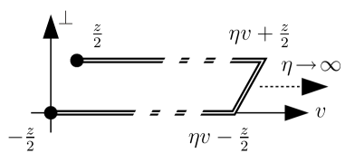
Figure 1: Path of the gauge connection $U$, cf. (3), in the correlator (2).

The operator in (2), extracting information about quark momentum from the proton state, is of the standard form used in the definition of transverse momentum-dependent parton distributions (TMDs) collbook ; ji04 ; aybat . The matrix element (2) only differs from the standard TMD correlator by the introduction of the nonvanishing momentum transfer $\Delta_{T}$ in the external states, defining a generalized TMD (GTMD) correlator mms in which the quark momentum information is supplemented by quark impact parameter information. Consequently, considerations from the standard TMD framework can be applied gtmdsoft in treating the TMD operator in (2). Physically, the staple-shaped gauge link path incorporates the effect of final state interactions on the struck quark in a semi-inclusive deep inelastic scattering (SIDIS) process. The staple legs represent semi-classical quark paths along which gluon exchanges with the proton remnant are summed. Generalized to the impact parameter-dependent case, the staple-shaped gauge link path thus incorporates into the quark orbital angular momentum the torque accumulated by the struck quark as it is leaving the proton burk . For $\eta=0$, this torque vanishes.

From the formal point of view, the TMD operator contains divergences that are absorbed into renormalization and soft factors in the standard TMD framework; these factors appear multiplicatively in the continuum theory collbook ; aybat ; gtmdsoft ; spl2 . They are identical for all four instances of $\Phi$ in (1) and the ratio is therefore designed to cancel them (of course, these factors do not depend on $\Delta_{T}$, which only enters through the external states). This is the chief motivation for forming the ratio (1) and employing the nonlocal operator with separation $a$ in the denominator; in this way, operators in the numerator and denominator match already at finite lattice spacing. Setting the number of valence quarks $n$ to the appropriate integer serves as the renormalization condition. Nonetheless, since the operator separations in (1) are proportional to the lattice spacing, additional ultraviolet divergences arise as the lattice spacing goes to zero. This is equivalent to the observation in momentum space that, even if one has constructed a renormalized TMD, $k_{T}$-moments thereof may still diverge as one lets $z_{T}$, which acts as a regulator on $k_{T}$-integrals, go to zero. The specific scheme to control that divergence adopted in (1) amounts to identifying the transverse momentum cutoff $z_{T}$ with the lattice resolution $a$. To connect (1) with its counterpart in other renormalization schemes such as the standard $\overline{MS}$ scheme, an additional matching would be required that is not available at present. The numerical results presented below suggest that this unquantified systematic uncertainty is minor. The scale evolution of quark orbital angular momentum has been discussed in detail recently in hatta_evol , giving an estimate of the variation expected in the regime in which the lattice calculation is performed. The numerical calculation to follow is carried out at a single lattice spacing $a$; it would be interesting to extend it to several lattice spacings to directly observe the scale evolution of the results.

It should be noted that the multiplicative nature of the renormalization factors in the continuum theory does not straightforwardly extend to the lattice theory. In general, the breaking of chiral symmetry engendered by the Wilson fermion discretization used in this work generates operator mixing within the class of TMD operators rentmd ; pertmix ; auxmix ; npmix that precludes a simple factoring out of renormalization factors and cancellation in the ratio (1). Also these effects will not be studied quantitatively in the present work, and they constitute a further systematic uncertainty. A study of the Sivers shift ratio rentmd , in which the same TMD operator appears as in (2), revealed no significant operator mixing effects at the level of statistical accuracy achieved in the calculation; that study included the gauge ensemble used also in the present work. This suggests that operator mixing effects also do not introduce a dominant systematic bias in the results obtained here.

A standard way to regulate the rapidity divergences rapidrev contained in the TMD operator for light-like staple direction $v$ is to take $v$ off the light cone into the spacelike region collbook ; aybat , while maintaining a zero transverse component, $v_{T}=0$. A convenient Lorentz-invariant way to characterize the direction of $v$ is the Collins-Soper type parameter

$$\hat{\zeta}=\frac{v\cdot P}{\sqrt{|v^{2}|}\sqrt{P^{2}}}$$ (4)

on which the numerical results obtained below will also depend. Ultimately, one is interested in their large-$\hat{\zeta}$ behavior; this corresponds to $v$ approaching the light cone. Choosing $v$ to be spacelike simultaneously facilitates a straightforward connection to the standard Lattice QCD methodology for evaluating hadronic matrix elements: Given that the temporal dimension in Lattice QCD is Euclidean, serving to project out the hadronic ground state, the operators of which one evaluates matrix elements cannot be extended in physical time. However, once a spacelike vector $v$ is adopted, the problem at hand can be boosted to a Lorentz frame in which $v$ is purely spatial, and thus the entire TMD operator in (2) exists at a single time. The lattice calculation can be performed in that frame. Maintaining $v_{T}=0$ in the lattice frame, $v$ will point purely in the (negative) 3-direction, $v\equiv-\vec{e}_{3}$. In that case, $\hat{\zeta}=P_{3}/m$ (where $m$ is the proton mass). Consequently, achieving large $\hat{\zeta}$ requires large proton momentum component $P_{3}$; this represents a significant challenge, cf. bmlat for a study in the context of the Boer-Mulders effect. On the other hand, in the special case $\eta=0$, the dependence on the staple direction $v$ disappears; Ji quark orbital angular momentum is boost-invariant. The corresponding results obtained below will indeed be seen to be independent of $P_{3}$ (or, equivalently, $\hat{\zeta}$, if one formally maintains $v\equiv-\vec{e}_{3}$ in the lattice frame).

On a lattice of finite extent with periodic boundary conditions in the spatial directions, momenta are quantized. Therefore, performing direct calculations only of the matrix element $\Phi(z_{T})$, cf. (2), limits the accuracy in determining its derivative with respect to $\Delta_{T}$, by forcing one to evaluate finite differences over, in practice, substantial momentum increments. In the initial study jitojm of quark orbital momentum in the proton employing the GTMD approach laid out here, this was the dominant source of systematic uncertainty. It introduced a bias in the overall magnitude of the numerical data approaching a factor 2. Although relative comparisons performed in jitojm , such as the one between Ji and Jaffe-Manohar orbital angular momentum, can be expected to be robust with respect to this bias, in absolute terms, the Ji orbital angular momentum extracted in jitojm displayed a significant discrepancy compared to the value obtained independently via Ji’s sum rule. To remedy this dominant systematic bias, and thereby achieve agreement with the result obtained via Ji’s sum rule within the statistical fluctuations, is the principal objective and advance of the present work. Other systematic uncertainties, such as the ones associated with renormalization discussed further above, are, in comparison, minor, and are accordingly deferred to future work.

To completely remove the systematic bias originating from finite difference evaluations of the $\Delta_{T}$-derivative of $\Phi(z_{T})$, a direct derivative method is adopted in the present work. The detailed implementation of the method will be described in the next section, following rome , where the method was first laid out in detail. Heuristically, the method is based on the observation that arbitrarily small increments in overall momenta can be achieved by twisting the spatial boundary conditions of the quarks, or, equivalently, coupling the quarks to a constant $U(1)$ background gauge field. For the purpose of computing a momentum derivative, this gauge field can be infinitesimally small, and can therefore be treated perturbatively. In effect, this generates an additional vector current insertion in the diagram one would calculate to obtain $\Phi(z_{T})$. Thus, by instead directly performing a lattice calculation of the diagram containing the additional vector current insertion, one directly accesses the $\Delta_{T}$-derivative of $\Phi(z_{T})$, excluding any systematic bias. A moderate price one pays is that the additional operator insertion will tend to somewhat increase the statistical fluctuations in the calculation.

III Lattice methodology

To obtain the proton matrix element $\Phi(z_{T})$, cf. (2), one calculates three-point functions $C_{\mbox{\scriptsize 3pt}}[\hat{O}]$ together with two-point functions $C_{\mbox{\scriptsize 2pt}}$, which are projected onto a definite proton momentum ${\bf p^{\prime}}={\bf P}+\boldsymbol{\Delta}_{T}/2$ at the proton sink, as well as a definite momentum transfer $\boldsymbol{\Delta}_{T}$ at the operator insertion in $C_{\mbox{\scriptsize 3pt}}[\hat{O}]$,

$$C_{\mbox{\scriptsize 3pt}}[\hat{O}](t,t_{f},{\bf p^{\prime}},{\bf p}) = \sum_{{\bf x}_{f},\,{\bf y}}e^{-i{\bf x}_{f}\cdot{\bf p^{\prime}}+i{\bf y}\cdot({\bf p^{\prime}-p})}\mbox{tr}[\Gamma_{\mbox{\scriptsize pol}}\langle n(t_{f},{\bf x}_{f})\hat{O}(t,{\bf y})\bar{n}(0,0)\rangle]$$ (5)

$$C_{\mbox{\scriptsize 2pt}}(t_{f},{\bf p^{\prime}}) = \sum_{{\bf x}_{f}}e^{-i{\bf x}_{f}\cdot{\bf p^{\prime}}}\mbox{tr}[\Gamma_{\mbox{\scriptsize pol}}\langle n(t_{f},{\bf x}_{f})\bar{n}(0,0)\rangle]\ .$$ (6)

By momentum conservation, a definite source momentum ${\bf p}={\bf P}-\boldsymbol{\Delta}_{T}/2$ is thereby implied in $C_{\mbox{\scriptsize 3pt}}[\hat{O}]$. The proton interpolating fields $n(t,{\bf x})$ are constructed in practice using Wuppertal-smeared quarks, to be discussed in more detail below, such as to optimize overlap with the true proton state. The projector $\Gamma_{\mbox{\scriptsize pol}}=\frac{1}{2}(1+\gamma_{4})\frac{1}{2}(1-i\gamma_{3}\gamma_{5})$ selects states polarized in the 3-direction. As already discussed further above, the lattice calculation is performed in a Lorentz frame in which the TMD operator $\hat{O}$, specified in (2), exists at the single time $t$; in particular, $v=-\vec{e}_{3}$, corresponding to $\hat{\zeta}=P_{3}/m$. In general, the three-point function $C_{\mbox{\scriptsize 3pt}}[\hat{O}]$ contains both connected contributions, in which $\hat{O}$ is inserted into a valence quark propagator, as well as disconnected contributions, in which $\hat{O}$ is inserted into a sea quark loop. In the present investigation, only the former are taken into account. The latter contributions, which are associated with significantly higher computational cost, are expected to be minor, and are excluded. In the isovector $u-d$ quark channel, the disconnected contributions cancel exactly; in that case, no systematic uncertainty is associated with neglecting the disconnected diagrams.

Having calculated the three-point and two-point functions, the matrix element (2) is obtained from the ratio

$$2E({\bf p^{\prime}})\frac{C_{\mbox{\scriptsize 3pt}}[\hat{O}](t,t_{f},{\bf p^{\prime}},{\bf p})}{C_{\mbox{\scriptsize 2pt}}(t_{f},{\bf p^{\prime}})}\longrightarrow\Phi(z_{T})$$ (7)

which exhibits plateaus in $t$ for $0\ll t\ll t_{f}$, yielding $\Phi(z_{T})$. Here, $E({\bf p})=E({\bf p^{\prime}})$ denotes the energy of the initial and final proton states. Note that, for general choices of initial and final momenta, the ratio (7) has to be replaced by a more general expression LHPC_1 ; LHPC_2 ; it is the specific symmetric choice of the initial and final momenta ${\bf p}={\bf P}-\boldsymbol{\Delta}_{T}/2$, ${\bf p^{\prime}}={\bf P}+\boldsymbol{\Delta}_{T}/2$ that allows one to use the simple ratio (7) here. For finite temporal separations, residual excited state contributions will contaminate the extraction of plateaus from (7). Control over these can be obtained by employing a sequence of source-sink separations $t_{f}$. In the present study, data for only one source-sink separation $t_{f}=1.14\,\mbox{fm}$ were gathered, and therefore it will not be possible to estimate excited state effects quantitatively. Previous form factor studies on the same gauge ensemble lhpc_ff1 ; lhpc_ff2 showed that the importance of excited state effects depends substantially on the specific observable considered. In some cases, the systematic bias at the separation $t_{f}=1.14\,\mbox{fm}$ was seen to be smaller than the statistical fluctuations, in other cases, it exceeded the latter by factors up to 2 to 3. Controlling for excited state effects will certainly be desirable in future investigations.

Consider now evaluating the $\Delta_{T}$-derivative of $\Phi(z_{T})$ at $\Delta_{T}=0$, as called for by (1). First, note that the two-point function $C_{\mbox{\scriptsize 2pt}}$ is an even function of $\boldsymbol{\Delta}_{T}$; therefore, only the derivative of the three-point function $C_{\mbox{\scriptsize 3pt}}[\hat{O}]$ is needed, while one can directly use $C_{\mbox{\scriptsize 2pt}}(t_{f},{\bf P})$ in (7). To proceed, it is useful to write $C_{\mbox{\scriptsize 3pt}}[\hat{O}]$ explicitly in terms of the appropriate propagators, combining the coordinates for ease of notation into four-vectors, e.g., $(t,{\bf y})\equiv y$,

$$C_{\mbox{\scriptsize 3pt}}[\hat{O}](t,t_{f},{\bf p^{\prime}},{\bf p})=\sum_{{\bf x}_{f},\,{\bf y}}e^{-i{\bf x}_{f}\cdot{\bf P}+i({\bf y}-{\bf x}_{f}/2)\cdot\boldsymbol{\Delta}_{T}}\cdot$$ (8)

$$\hskip 25.6073pt\cdot\left\langle\mbox{tr}\left[S_{\Gamma_{\mbox{\tiny pol}}}^{n\bar{n}}(0;x_{f})G_{\mbox{\scriptsize sm-pt}}(x_{f},y-z_{T}/2)\gamma^{+}U(y-z_{T}/2,y+z_{T}/2)G_{\mbox{\scriptsize pt-sm}}(y+z_{T}/2,0)\right]\right\rangle$$

$$\hskip 82.51282pt=\sum_{{\bf x}_{f},\,{\bf y}}e^{-i{\bf x}_{f}\cdot{\bf P}}\ e^{-i({\bf x}_{f}-({\bf y}-{\bf z}_{T}/2))\cdot\boldsymbol{\Delta}_{T}/2}\ e^{i({\bf y}+{\bf z}_{T}/2)\cdot\boldsymbol{\Delta}_{T}/2}\cdot$$ (9)

$$\hskip 25.6073pt\cdot\left\langle\mbox{tr}\left[\left(\gamma_{5}G_{\mbox{\scriptsize pt-sm}}(y-z_{T}/2,x_{f})\gamma_{5}S_{\Gamma_{\mbox{\tiny pol}}}^{n\bar{n}\,\dagger}(0;x_{f})\right)^{\dagger}\gamma^{+}U(y-z_{T}/2,y+z_{T}/2)G_{\mbox{\scriptsize pt-sm}}(y+z_{T}/2,0)\right]\right\rangle$$

$$\hskip 82.51282pt=\sum_{{\bf x}_{f},\,{\bf y}}e^{-i{\bf x}_{f}\cdot{\bf P}}\cdot$$ (10)

$$\hskip 25.6073pt\cdot\left\langle\mbox{tr}\left[\left(\gamma_{5}G_{\mbox{\scriptsize pt-sm}}(y-z_{T}/2,x_{f};\boldsymbol{\Delta}_{T}/2)\gamma_{5}S_{\Gamma_{\mbox{\tiny pol}}}^{n\bar{n}\,\dagger}(0;x_{f})\right)^{\dagger}\gamma^{+}U(y-z_{T}/2,y+z_{T}/2)G_{\mbox{\scriptsize pt-sm}}(y+z_{T}/2,0;-\boldsymbol{\Delta}_{T}/2)\right]\right\rangle.$$

Here, $S_{\Gamma_{\mbox{\tiny pol}}}^{n\bar{n}}$ denotes the standard sequential source formed at the sink time $t_{f}$, as described in detail, e.g., in the Appendix of dolgov ; $G_{\mbox{\scriptsize pt-sm}}(r,s)$ is the standard quark propagator from a smeared source to a point sink. In the second step, the $\gamma_{5}$-hermiticity of the propagators was used, and in the third step, the twisted propagator

$$G_{\mbox{\scriptsize pt-sm}}(r,s;{\bf q})=e^{-i({\bf r}-{\bf s})\cdot{\bf q}}G_{\mbox{\scriptsize pt-sm}}(r,s)$$ (11)

was introduced. Thus, the $\Delta_{T}$-dependence has been entirely absorbed into the twisted propagators, and it is their derivatives one needs in order to obtain the $\Delta_{T}$-derivative of $C_{\mbox{\scriptsize 3pt}}[\hat{O}]$. Following rome ; nhasan , in the absence of smearing, the derivative of the twisted point-to-point propagator can be cast in the form

$$\left.\frac{\partial}{\partial q^{j}}G_{\mbox{\scriptsize pt-pt}}(r,s;{\bf q})\right|_{{\bf q}=0}=-i\sum_{z}G_{\mbox{\scriptsize pt-pt}}(r,z)\Gamma_{V}^{j}G_{\mbox{\scriptsize pt-pt}}(z,s)$$ (12)

where the sum extends over the four-dimensional coordinate $z$, and the vector current insertion acts as

$$\Gamma_{V}^{j}G_{\mbox{\scriptsize pt-pt}}(z,s)=U^{\dagger}_{j}(z-\vec{e}_{j})\frac{1+\gamma^{j}}{2}G_{\mbox{\scriptsize pt-pt}}(z-\vec{e}_{j},s)-U_{j}(z)\frac{1-\gamma^{j}}{2}G_{\mbox{\scriptsize pt-pt}}(z+\vec{e}_{j},s)\ .$$ (13)

Supplementing the point-to-point propagator with a smearing kernel,

$$G_{\mbox{\scriptsize pt-sm}}(r,s;{\bf q})=e^{-i({\bf r}-{\bf s})\cdot{\bf q}}\sum_{u}G_{\mbox{\scriptsize pt-pt}}(r,u)K(u,s)=\sum_{u}G_{\mbox{\scriptsize pt-pt}}(r,u;{\bf q})K(u,s;{\bf q})$$ (14)

where also the twisted smearing kernel

$$K(u,s;{\bf q})=e^{-i({\bf u}-{\bf s})\cdot{\bf q}}K(u,s)$$ (15)

has been introduced, one has the derivative

$$\left.\frac{\partial}{\partial q^{j}}G_{\mbox{\scriptsize pt-sm}}(r,s;{\bf q})\right|_{{\bf q}=0}=\sum_{z}G_{\mbox{\scriptsize pt-pt}}(r,z)\left[-i\sum_{u}\Gamma_{V}^{j}G_{\mbox{\scriptsize pt-pt}}(z,u)K(u,s)+\left.\frac{\partial}{\partial q^{j}}K(z,s;{\bf q})\right|_{{\bf q}=0}\right]$$ (16)

where the derivative of the twisted smearing kernel will be treated below. Thus, in order to calculate the $\Delta_{T}$-derivative of $C_{\mbox{\scriptsize 3pt}}[\hat{O}]$, one has to evaluate two additional propagators compared to a standard calculation of $C_{\mbox{\scriptsize 3pt}}[\hat{O}]$ itself. In the latter case, one needs to evaluate the forward propagator from a smeared source $K$, and the backward propagator from the smeared sequential source $K\gamma_{5}S_{\Gamma_{\mbox{\tiny pol}}}^{n\bar{n}\dagger}$; now, one additionally needs propagators from the sources

$$-i\Gamma_{V}^{j}G_{\mbox{\scriptsize pt-pt}}K+\left.\frac{\partial}{\partial q^{j}}K\right|_{{\bf q}=0}\ ,\ \ \ \ \ \ \ \ \ \ \ \ \ \ -i\Gamma_{V}^{j}G_{\mbox{\scriptsize pt-pt}}K\gamma_{5}S_{\Gamma_{\mbox{\tiny pol}}}^{n\bar{n}\dagger}+\left(\left.\frac{\partial}{\partial q^{j}}K\right|_{{\bf q}=0}\right)\gamma_{5}S_{\Gamma_{\mbox{\tiny pol}}}^{n\bar{n}\dagger}\ .$$ (17)

It remains to construct the derivative of the twisted smearing kernel nhasan . A single step of (twisted) Wuppertal smearing is defined by

$$K_{0}(u,s;{\bf q}) = e^{-i({\bf u}-{\bf s})\cdot{\bf q}}\frac{1}{1+6\alpha}\left(\delta_{u,s}+\alpha\sum_{j=1}^{3}\left[U_{j}(u)\delta_{u+\vec{e}_{j},s}+U^{\dagger}_{j}(u-\vec{e}_{j})\delta_{u-\vec{e}_{j},s}\right]\right)$$ (18)

$$= \frac{1}{1+6\alpha}\left(\delta_{u,s}+\alpha\sum_{j=1}^{3}\left[e^{iq^{j}}U_{j}(u)\delta_{u+\vec{e}_{j},s}+e^{-iq^{j}}U^{\dagger}_{j}(u-\vec{e}_{j})\delta_{u-\vec{e}_{j},s}\right]\right)$$ (19)

so that its derivative at zero momentum is

$$K_{0}^{\prime}(u,s)\equiv\left.\frac{\partial}{\partial q^{j}}K_{0}(u,s;{\bf q})\right|_{{\bf q}=0}=\frac{\alpha}{1+6\alpha}\left[iU_{j}(u)\delta_{u+\vec{e}_{j},s}-iU^{\dagger}_{j}(u-\vec{e}_{j})\delta_{u-\vec{e}_{j},s}\right]\ .$$ (20)

If the smearing kernel $K$ is given by $N$ steps of Wuppertal smearing,

$$K(u,s;{\bf q})=\sum_{w_{1},w_{2},\ldots,w_{N-1}}K_{0}(u,w_{1};{\bf q})K_{0}(w_{1},w_{2};{\bf q})\ldots K_{0}(w_{N-1},s;{\bf q})$$ (21)

then its derivative at zero momentum can be computed iteratively as

$$K^{\prime}\equiv(K_{0}^{N})^{\prime}=K_{0}^{\prime}K_{0}^{N-1}+K_{0}(K_{0}^{N-1})^{\prime}\ .$$ (22)

The numerical data for the present study were generated using a 2+1-flavor isotropic clover fermion ensemble on $32^{3}\times 96$ lattices generated by R. Edwards, B. Joó and K. Orginos with lattice spacing $a=0.114\,\mbox{fm}$ and pion mass $m_{\pi}=317\,\mbox{MeV}$. The present investigation is therefore also significantly closer to the physical limit than the initial exploration jitojm . A total of 23224 data samples was gathered on 968 gauge configurations. The Euclidean temporal separation between proton sources and sinks was $t_{f}=10a$. HYP-smearing was applied to the lattice links used in constructing the Wilson line $U$ in (2). This leads to the renormalization and soft factors associated with the operator in (2) corresponding more closely to their tree-level values even before their cancellation in the ratio (1). Three spatial proton momenta were used, ${\bf P}\cdot L/(2\pi)=(0,0,n_{P})$ with $n_{P}=0,1,2$, where $L=32a$ denotes the spatial lattice extent. Although the corresponding range of the Collins-Soper parameter $\hat{\zeta}=0,0.315,0.63$ is limited, and one cannot a priori expect to obtain a good indication of the large-$\hat{\zeta}$ behavior with data in this range, it will be seen below that the results for Jaffe-Manohar orbital angular momentum already appear to stabilize in the region of the two nonzero values of $\hat{\zeta}$. Corroboration concerning this suggested early onset of asymptotic behavior by future studies including larger $\hat{\zeta}$ would certainly be desirable.

IV Numerical results

Considering initially the special case of a straight Wilson line, $\eta=0$, corresponding to Ji quark orbital angular momentum, Fig. 2 displays the results obtained in the isovector case at the three available values of $\hat{\zeta}$. Recall that $\hat{\zeta}$ is defined here through $v=-\vec{e}_{3}$ in the lattice frame even when $\eta=0$; with that definition, on the other hand, Ji quark orbital angular momentum should then be independent of $\hat{\zeta}$, since $v$ does not in fact enter its construction. This is borne out by the data in Fig. 2. The residual apparent trend in the data may be due to the deviation between the lattice dispersion relation and the continuum dispersion relation used in the data analysis, but is also consistent with statistical fluctuation.

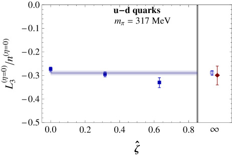
Figure 2: Ji quark orbital angular momentum, i.e., the $\eta=0$ limit, for the three values of $\hat{\zeta}$ probed, with the average plotted at $\hat{\zeta}=\infty$ (open square). The filled diamond represents the value extracted at the same pion mass in the $\overline{MS}$ scheme at the scale $\mu^{2}=4\,\mbox{GeV}^{2}$ via Ji’s sum rule LHPC_2 . The isovector $u-d$ quark combination was evaluated. The shown uncertainties are statistical jackknife errors.

Performing a $\chi^{2}$ fit of a constant in $\hat{\zeta}$ to the data yields the average value plotted at $\hat{\zeta}=\infty$, taken here to label the physical limit. This result is confronted with an independent lattice determination of Ji quark orbital angular momentum via Ji’s sum rule at the same pion mass, in the $\overline{MS}$ scheme at the scale $\mu^{2}=4\,\mbox{GeV}^{2}$ LHPC_2 . The two determinations are in good agreement; the discrepancy observed in the initial exploration jitojm is entirely resolved. This validates the use of the GTMD approach, properly implemented in particular with respect to taking the $\Delta_{T}$-derivative in (1), to calculating quark orbital angular momentum in the proton. The result corroborates the assumption that the various further systematic uncertainties noted above, i.e., stemming from renormalization and matching, operator mixing, or excited state contaminations are minor and do not bias the result beyond the statistical uncertainty.

Departing from the $\eta=0$ limit, one probes the torque burk due to final state interactions accumulated by a quark struck in a deep inelastic scattering process as it exits the proton. The $\eta=\pm\infty$ limit corresponds to Jaffe-Manohar orbital angular momentum. By varying $\eta$ gradually, a gauge-invariant, continuous interpolation between the Ji and Jaffe-Manohar limits can be exhibited. This is shown in Fig. 3, again for the isovector $u-d$ quark channel, and for the three values of $\hat{\zeta}$ probed. Note that the plots are normalized to the magnitude of the Ji quark orbital angular momentum, i.e., the result obtained at $\eta=0$.

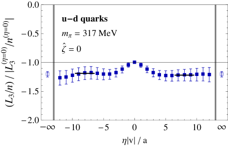
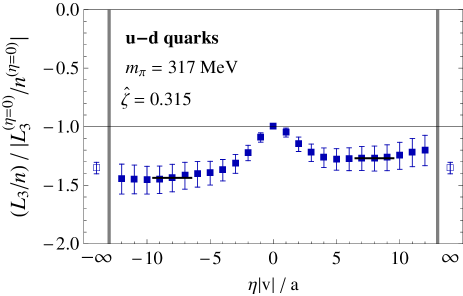
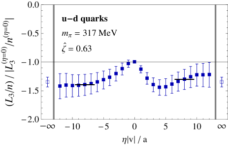
Figure 3: Quark orbital angular momentum as a function of staple length parameter $\eta$, normalized to the magnitude of Ji quark orbital angular momentum, i.e., the result obtained at $\eta=0$. This quantity is even under $\eta\rightarrow-\eta$, corresponding to time reversal. Accordingly, the $|\eta|\rightarrow\infty$ extrapolated values are obtained by averaging the $\eta>0$ and $\eta<0$ plateaus, which are determined by fitting to the $|\eta||v|/a=7,\ldots,9$ range. The isovector $u-d$ quark combination is shown, with the three panels corresponding to the three available values of $\hat{\zeta}$. The shown uncertainties are statistical jackknife errors.

Evidently, the torque supplied by the final state interactions is appreciable, as already observed in jitojm . Compared to the initial Ji value, quark orbital angular momentum is enhanced in magnitude as one proceeds towards the asymptotic Jaffe-Manohar limit. Contrasting the three panels in Fig. 3, the effect strengthens as the Collins-Soper parameter $\hat{\zeta}$ is increased, with Jaffe-Manohar quark orbital angular momentum enhanced by about 30% relative to the Ji case for the two nonzero values of $\hat{\zeta}$. This is somewhat less strong than in the exploration jitojm ; whether this is a genuine physical trend associated with the change in pion mass from $518\,\mbox{MeV}$ to $317\,\mbox{MeV}$, or whether it is an artefact of the systematic bias in the calculation in jitojm cannot be decided at this point. The fact that the effect strengthens with rising $\hat{\zeta}$ suggests that it can be expected to persist into the $\hat{\zeta}\rightarrow\infty$ limit. Fig. 4 displays the integrated torque, i.e., the difference between the Jaffe-Manohar and Ji quark orbital momenta,

$$\tau_{3}=\frac{L^{(\eta=\infty)}_{3}}{n^{(\eta=\infty)}}-\frac{L^{(\eta=0)}_{3}}{n^{(\eta=0)}}\ ,$$ (23)

as a function of $\hat{\zeta}$, normalized to the magnitude of Ji quark orbital momentum. An extrapolation to the $\hat{\zeta}\rightarrow\infty$ limit is also shown. The ad hoc fit ansatz, $A+B/\hat{\zeta}$, is not underpinned by a theoretical argument at this point, but is motivated by the good description it provides of the considerably more detailed data as a function of $\hat{\zeta}$ available for the pion Boer-Mulders TMD ratio bmlat . Auxiliary information concerning the expected large-$\hat{\zeta}$ behavior would be desirable to aid in sharpening the analysis. The ad hoc extrapolation indeed yields a signal in the $\hat{\zeta}\rightarrow\infty$ limit.

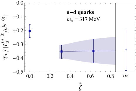
Figure 4: Integrated torque accumulated by a quark struck in a deep inelastic scattering process along its trajectory exiting the proton, as a function of Collins-Soper parameter $\hat{\zeta}$. The data pertain to the isovector $u-d$ quark channel, and are normalized to the magnitude of the $\eta=0$ Ji orbital angular momentum. An ad hoc extrapolation to the $\hat{\zeta}\rightarrow\infty$ limit is also exhibited. The shown uncertainties are statistical jackknife errors.

Generalizing to the flavor-separated case, it should be kept in mind that the additional disconnected contributions that arise compared to the isovector case have not been evaluated. These are, however, expected to be minor at the pion mass $m_{\pi}=317\,\mbox{MeV}$ used in this calculation. Fig. 5 shows data analogous to Fig. 3 for one value of $\hat{\zeta}$, exhibiting the behavior of $d$-quark and $u$-quark orbital angular momentum separately, as well as the total (isoscalar) quark orbital angular momentum. Here, the $u$-quark data have been normalized to two quarks, i.e., $L_{3}/n$ in the $u$ quark case has been multiplied by 2 to compensate for $n=2$ for $u$ quarks; hence the “$2u$” label. The isoscalar result was then obtained by simple addition of the “$d$” and “$2u$” data.

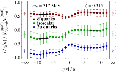
Figure 5: Flavor-separated quark orbital angular momentum as a function of staple length $\eta$, analogous to Fig. 3, at fixed $\hat{\zeta}=0.315$. Results are displayed for $d$ quarks and for two $u$ quarks (i.e., the $u$-quark data for $L_{3}/n$ have been multiplied by $2$ to compensate for $n=2$), as well as for the isoscalar total quark orbital angular momentum, i.e., the sum of the “$d$” and “$2u$” data. All results are still normalized by the magnitude of isovector Ji orbital angular momentum (thus, at $\eta=0$, the “$2u$” and “$d$” data differ by unity). The shown uncertainties are statistical jackknife errors.

As observed previously in jitojm , the strong cancellation of the $u$- and $d$-quark orbital angular momenta in the proton that has long been known for the $\eta=0$ Ji case LHPC_1 ; LHPC_2 extends to nonzero $\eta$ and the Jaffe-Manohar limit. Only a small negative contribution to the spin of the proton from quark orbital angular momentum remains. The data for the flavor-separated integrated torque, cf. (23), are collected in Fig. 6 and extrapolated to the $\hat{\zeta}\rightarrow\infty$ limit. At the present level of statistics, scarcely a signal is obtained for the flavor-separated integrated torque in that limit; the data do appear compatible with the observations made at fixed $\hat{\zeta}=0.315$ from Fig. 5.

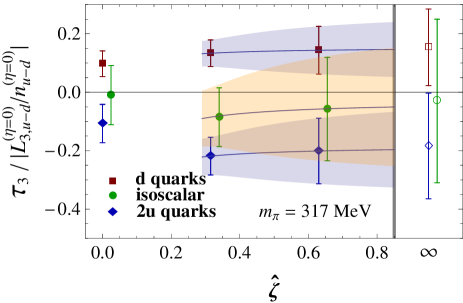
Figure 6: Flavor-separated integrated torque accumulated by a quark struck in a deep inelastic scattering process, as a function of $\hat{\zeta}$, analogous to Fig. 4, together with ad hoc extrapolations to infinite $\hat{\zeta}$. Data for $d$ quarks, for two $u$ quarks (i.e., the $u$-quark data for $\tau_{3}$ have been multiplied by $2$ to compensate for $n=2$ in the $u$-quark case), and their sum, the isoscalar $u+d$ quark combination, are shown. Data are normalized by the magnitude of isovector Ji quark orbital angular momentum, as in previous figures. For better visibility, isoscalar data are slightly displaced horizontally. The shown uncertainties are statistical jackknife errors.

V Conclusions and outlook

The chief advance of the present study is the adoption of a direct derivative method rome in the GTMD approach to evaluating quark orbital angular momentum in the proton in Lattice QCD. The introduction of this method has led to a reliable quantitative computation of the needed derivative, with respect to momentum transfer, of the relevant GTMD matrix element. This is validated by the result obtained specifically for the quark orbital angular momentum defined through the Ji decomposition of proton spin; it agrees well with the corresponding result obtained independently in Lattice QCD calculations relying on Ji’s sum rule LHPC_2 . The discrepancy observed in the initial exploration jitojm is thus resolved.

The agreement between the quark orbital angular momentum calculated in this work using the GTMD approach and the result from the Ji sum rule suggests that other systematic uncertainties, such as ones associated with excited state effects, renormalization and matching, as well as operator mixing are minor and do not rise to the level of the statistical uncertainties of the present calculation.

In the GTMD approach, one directly computes quark orbital angular momentum by weighting the appropriate Wigner function (related to GTMDs via Fourier transformation) by $b_{T}\times k_{T}$, where $b_{T}$ is the quark impact parameter and $k_{T}$ the quark transverse momentum lorce ; leader . The aforementioned derivative with respect to momentum transfer supplies the weighting by $b_{T}$, its Fourier conjugate. The information on $k_{T}$, on the other hand, is supplied through the nonlocal TMD operator used in constructing the relevant proton matrix element (2). The treatment of renormalization issues thus follows closely the methods used in more widely explored Lattice TMD calculations straightlett ; straightlinks ; tmdlat ; bmlat ; rentmd . Ratios of proton matrix elements are constructed to cancel renormalization and soft factors associated with the TMD operator. In effect, one evaluates quark orbital angular momentum in units of the number of valence quarks. Operator mixing effects rentmd ; pertmix ; auxmix ; npmix can spoil these cancellations, and though they appear not to play a significant role in the present calculation, these effects will ultimately have to be brought under control.

The advantage of this nonlocal operator-based GTMD approach is that one can extend Lattice QCD calculations beyond the Ji decomposition of proton spin and establish a continuous, gauge-invariant interpolation from Ji jidecomp to Jaffe-Manohar jmdecomp quark orbital angular momentum. The corresponding information is contained in the choice of Wilson line path in the TMD operator. A straight Wilson line path yields Ji quark orbital angular momentum jist ; burk ; eomlir , and a staple-shaped Wilson line path, in the limit of infinite staple length, yields its Jaffe-Manohar counterpart hatta ; burk . The difference between the two can be interpreted as the integrated torque accumulated by a quark struck in a deep inelastic scattering process as it exits the proton, through final state interactions burk . It corresponds to a Qiu-Sterman type correlator burk ; eomlir ; eomlong . The data obtained for this term in the present investigation allow one to observe the gradual accumulation of torque by the quark until it attains the asymptotic Jaffe-Manohar orbital angular momentum. The latter is enhanced in magnitude relative to the initial Ji value, with the integrated torque adding about one third of the magnitude of the Ji orbital angular momentum at the pion mass $m_{\pi}=317\,\mbox{MeV}$ used in this calculation.

To further sharpen the analysis of quark orbital angular momentum within the GTMD approach, calculations for a sequence of lattice spacings would be desirable, to allow for a direct study of the scale evolution. Also, a more comprehensive exploration of the dependence on the Collins-Soper parameter $\hat{\zeta}$ is warranted, to clarify whether the results indeed already stabilize at the fairly low values of $\hat{\zeta}$ employed in this work, as suggested by Fig. 4. Ultimately, the large $\hat{\zeta}$ behavior determines the physical limit. Finally, of course, also further progress towards the physical pion mass must be made.

The improved calculation of quark orbital angular momentum based on GTMDs achieved using the present methodology opens the way to reliably compute other related quantities, such as quark spin-orbit correlations in the proton lorce ; eomlong . Corresponding calculations are in progress, employing domain wall fermions to curtail the operator mixing effects that are induced when the fermion discretization breaks chiral symmetry.

References

- (1) J. Ashman et al. [European Muon Collaboration], Phys. Lett. B206, 364 (1988).
- (2) J. Ashman et al. [European Muon Collaboration], Nucl. Phys. B328, 1 (1989).
- (3) X. Ji, Phys. Rev. Lett. 78, 610 (1997).
- (4) H.-W. Lin, R. Gupta, B. Yoon, Y.-C. Jang and T. Bhattacharya, Phys. Rev. D 98, 094512 (2018).
- (5) J. Liang, Y.-B. Yang, T. Draper, M. Gong and K.-F. Liu, Phys. Rev. D 98, 074505 (2018).
- (6) P. Hägler et al. [LHP Collaboration], Phys. Rev. D 77, 094502 (2008).
- (7) J. D. Bratt et al. [LHP Collaboration], Phys. Rev. D 82, 094502 (2010).
- (8) M. Göckeler, R. Horsley, D. Pleiter, P. E. L. Rakow, A. Schäfer, G. Schierholz and W. Schroers [QCDSF Collaboration], Phys. Rev. Lett. 92, 042002 (2004).
- (9) G. Bali, S. Collins, M. Göckeler, R. Rödl, A. Schäfer and A. Sternbeck [RQCD Collaboration], Phys. Rev. D 100, 014507 (2019).
- (10) M. Deka, T. Doi, Y.-B. Yang, B. Chakraborty, S. J. Dong, T. Draper, M. Glatzmaier, M. Gong, H.-W. Lin, K.-F. Liu, D. Mankame, N. Mathur and T. Streuer, Phys. Rev. D 91 (2015), 014505 (2015).
- (11) C. Alexandrou, M. Constantinou, K. Hadjiyiannakou, K. Jansen, C. Kallidonis, G. Koutsou, A. Vaquero Avilés-Casco and C. Wiese, Phys. Rev. Lett. 119, 142002 (2017).
- (12) C. Alexandrou, S. Bacchio, M. Constantinou, J. Finkenrath, K. Hadjiyiannakou, K. Jansen, G. Koutsou, H. Panagopoulos and G. Spanoudes, Phys. Rev. D 101, 094513 (2020).
- (13) Y.-B. Yang, R. S. Sufian, A. Alexandru, T. Draper, M. J. Glatzmaier, K.-F. Liu and Y. Zhao, Phys. Rev. Lett. 118, 102001 (2017).
- (14) R. Jaffe and A. Manohar, Nucl. Phys. B337, 509 (1990).
- (15) S. Meißner, A. Metz and M. Schlegel, JHEP 0908, 056 (2009).
- (16) C. Lorcé and B. Pasquini, Phys. Rev. D 84, 014015 (2011).
- (17) E. Leader and C. Lorcé, Phys. Rept. 541, 163 (2014).
- (18) Y. Hatta, Phys. Lett. B708, 186 (2012).
- (19) X. Ji, X. Xiong and F. Yuan, Phys. Rev. Lett. 109, 152005 (2012).
- (20) M. Burkardt, Phys. Rev. D 88, 014014 (2013).
- (21) A. Rajan, A. Courtoy, M. Engelhardt and S. Liuti, Phys. Rev. D 94, 034041 (2016).
- (22) A. Rajan, M. Engelhardt and S. Liuti, Phys. Rev. D 98, 074022 (2018).
- (23) M. Engelhardt, Phys. Rev. D 95, 094505 (2017).
- (24) P. Hägler, B. Musch, J. W. Negele and A. Schäfer, Europhys. Lett. 88, 61001 (2009).
- (25) B. Musch, P. Hägler, J. W. Negele and A. Schäfer, Phys. Rev. D 83, 094507 (2011).
- (26) B. Musch, P. Hägler, M. Engelhardt, J. Negele and A. Schäfer, Phys. Rev. D 85, 094510 (2012).
- (27) M. Engelhardt, P. Hägler, B. Musch, J. Negele and A. Schäfer, Phys. Rev. D 93, 054501 (2016).
- (28) B. Yoon, M. Engelhardt, R. Gupta, T. Bhattacharya, J. Green, B. Musch, J. Negele, A. Pochinsky, A. Schäfer, and S. Syritsyn, Phys. Rev. D 96, 094508 (2017).
- (29) J. C. Collins, Foundations of Perturbative QCD (Cambridge University Press, 2011).
- (30) X. Ji, J.-P. Ma and F. Yuan, Phys. Rev. D 71, 034005 (2005).
- (31) S. M. Aybat and T. Rogers, Phys. Rev. D 83, 114042 (2011).
- (32) M. Echevarria, A. Idilbi, K. Kanazawa, C. Lorcé, A. Metz, B. Pasquini and M. Schlegel, Phys. Lett. B759, 336 (2016).
- (33) S. M. Aybat, J. C. Collins, J.-W. Qiu and T. C. Rogers, Phys. Rev. D 85, 034043 (2012).
- (34) Y. Hatta and X. Yao, Phys. Lett. B798, 134941 (2019).
- (35) M. Constantinou, H. Panagopoulos and G. Spanoudes, Phys. Rev. D 99, 074508 (2019).
- (36) J. R. Green, K. Jansen and F. Steffens, Phys. Rev. D 101, 074509 (2020).
- (37) P. Shanahan, M. Wagman and Y. Zhao, Phys. Rev. D 101, 074505 (2020).
- (38) J. C. Collins, T. C. Rogers and A. M. Stasto, Phys. Rev. D 77, 085009 (2008).
- (39) G. M. de Divitiis, R. Petronzio and N. Tantalo, Phys. Lett. B718, 589 (2012).
- (40) J. R. Green, S. Meinel, M. Engelhardt, S. Krieg, J. Laeuchli, J. Negele, K. Orginos, A. Pochinsky and S. Syritsyn, Phys. Rev. D 92, 031501 (2015).
- (41) J. R. Green, N. Hasan, S. Meinel, M. Engelhardt, S. Krieg, J. Laeuchli, J. Negele, K. Orginos, A. Pochinsky and S. Syritsyn, Phys. Rev. D 95, 114502 (2017).
- (42) N. Hasan, J. Green, S. Meinel, M. Engelhardt, S. Krieg, J. Negele, A. Pochinsky and S. Syritsyn, Phys. Rev. D 97, 034504 (2018).
- (43) D. Dolgov, R. Brower, S. Capitani, P. Dreher, J. Negele, A. Pochinsky, D. Renner, N. Eicker, T. Lippert, K. Schilling, R. Edwards and M. Heller [LHP and SESAM Collaborations], Phys. Rev. D 66, 034506 (2002).
- (44) R. G. Edwards and B. Joó [SciDAC Collaboration], Nucl. Phys. Proc. Suppl. 140, 832 (2005).
-
(45)
A. Pochinsky, Qlua,
https://usqcd.lns.mit.edu/qlua.