Recent Advances and New Guidelines on Hyperspectral and Multispectral Image Fusion
Abstract
Hyperspectral image (HSI) with high spectral resolution often suffers from low spatial resolution owing to the limitations of imaging sensors. Image fusion is an effective and economical way to enhance the spatial resolution of HSI, which combines HSI with higher spatial resolution multispectral image (MSI) of the same scenario. In the past years, many HSI and MSI fusion algorithms are introduced to obtain high-resolution HSI. However, it lacks a full-scale review for the newly proposed HSI and MSI fusion approaches. To tackle this problem, this work gives a comprehensive review and new guidelines for HSI-MSI fusion. According to the characteristics of HSI-MSI fusion methods, they are categorized as four categories, including pan-sharpening based approaches, matrix factorization based approaches, tensor representation based approaches, and deep convolution neural network based approaches. We make a detailed introduction, discussions, and comparison for the fusion methods in each category. Additionally, the existing challenges and possible future directions for the HSI-MSI fusion are presented.
keywords:
Hyperspectral and multispectral image fusion , Hyperspectral image super-resolution , Hyperspectral imaging1 Introduction
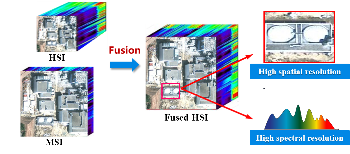
Hyperspectral imaging sensor can collect dozens of or hundreds of spectral bands in wide range spectral coverage. Since the materials often have different reflectance for different wavelength, hyperspectral image (HSI) enables accurate identification of materials owing to its high spectral resolution and wide spectral range. In this way, hyperspectral imaging has found comprehensive applications on remote sensing [1], face recognition [2], medical diagnosis [3], etc. However, on account of limitations for imaging cameras, there is the certain tradeoff for the spectral resolution and spatial resolution. Hence, HSI with a large number of bands usually has a low spatial resolution to ensure high SNR. On the contrary, imaging sensors can obtain an image with a higher spatial resolution but with a small number of spectral bands, consisting of RGB image, panchromatic image, and multispectral image (MSI). As shown in Table 1, spaceborne imaging sensor can acquire the high-resolution panchromatic image and four-band MSI with decimetric spatial resolution and metric spatial resolution, respectively. However, HSI can only be acquired with a spatial resolution of dozens of meters, which hinders the applications of HSI. One effectual and economical way to improve the spatial resolution of HSI is image fusion. More and more sensors can simultaneously acquire HSI and high-resolution MSI on the same scenario, and therefore image fusion approaches can be performed to acquire a fused image with the high spectral resolution and high spatial resolution, which is referred to as HSI-MSI fusion. For example, Hyperspectral imager suite (HISUI), the Japanese next-generation earth-observing sensor, simultaneity has hyperspectral and multispectral imaging sensor, where the spatial resolution of HSI and MSI are 30m and 5m, respectively. Gaofen (GF)-5 satellite and Gaofen (GF)-2 satellite, designed by China, takes the hyperspectral imaging and multispectral imaging sensors, respectively, where the HSI and MSI have the ground sampling distance (GSD) of 30m and 4m, respectively. As illustrated in Figure 1, HSI and MSI fusion is an effective and common way to improve the spatial resolution of the HSI. The HSI and MSI fusion is the part of pixel-level image fusion [4, 5, 6, 7, 8, 9, 10, 11, 12, 13]. The fused image of high spatial and spectral resolution can help us better recognize and understand the materials, which has contributed to many tasks including object classification [14], anomaly detection [15], change detection [16], etc. Reference [15] shows that the fused HSI indeed improves the detection accuracy compared with the original HSI. The fusion technique can find application in high spatial resolution ecosystem monitoring, minerals survey, plant investigation, and disaster warning.
| Sensor | Spectral range (nm) | Number of bands | GSD (m) | ||
|---|---|---|---|---|---|
| HYPXIM |
|
400-2500 | 210 | 8 | |
|
400-800 | 1 | 2 | ||
| HISUI |
|
400-2500 | 185 | 30 | |
|
450-900 | 4 | 5 | ||
| GF-5 |
|
400-2500 | 330 | 30 | |
| GF-2 |
|
450-900 | 4 | 4 | |
| WorldView-2 |
|
450-900 | 4 | 2 | |
| Hyperion |
|
400-2500 | 220 | 4 | |
Recently, a number of approaches have been presented to fuse the HSI and MSI. However, it lacks critical discussions for newly proposed HSI-MSI fusion methods. Vivone et al. [17] give a review and comparison for the pan-sharpening approach, and pan-sharpening is a special instance of the HSI-MSI fusion. This reference mainly focuses on the traditional component substitution (CS) methods and multi-resolution analysis (MRA) methods. Later, Loncan et al. [18] present a study of the HSI-MSI fusion methods, which compares the newly proposed matrix factorization (MF) based fusion methods with traditional pan-sharpening approaches. More recently, Yokyao et al. [19] give the comparative study for more newly proposed HSI-MSI fusion methods, and select ten representative works for comparison. However, the recently proposed tensor based fusion approaches and deep convolution neural network (CNN) based approaches are not considered.
In this article, we give a comprehensive review for the HSI-MSI fusion approaches. In specific, HSI-MSI fusion methods are categorized as four classes, including methods extended by pan-sharpening, MF based methods, tensor representation (TR) based methods, and deep CNN based methods. Furthermore, we give a detailed introduction to these methods and clarify their characteristics, advantages, and limitations. What is more, we also introduce the challenges and guidelines for HSI-MSI fusion. Compared with the previous works, we give the more detailed introduction to the recent progress in HSI-MSI fusion, especially on the tensor based fusion methods and deep CNN based approaches.
The remainder of this paper is organized as follows. Section II introduces the notations. In Section III, we review the representative HSI super-resolution literature. Section VI introduces the experimental comparison for the representative fusion methods, Section V introduces the challenges and possible research direction for HSI-MSI fusion. Section VI concludes the paper.
2 Notations
Before introducing different HSI-MSI fusion methods, we firstly give notations for the HSI and MSI. The high-resolution HSI, low-resolution HSI, and high-resolution MSI are represented by tensors, and are denoted by , , and , respectively. The first and second modes of tensor index the spatial dimension, and the third mode of the tensor indexes spectral dimension. is the matrix obtained by unfolding the tensor -dimensional tensor along -th mode.
Tensor product: The -mode product of tensor and matrix is written as
| (1) |
where , and it is equivalent to the following equation
| (2) |
Tucker Decomposition: Based on the Tucker decomposition [20], tensor can be factored as
| (3) |
in which denotes factor matrix in -th mode, and is the core tensor.
3 HSI-MSI Fusion Methods
According to the characteristics of HSI-MSI fusion approaches, they can be classified into four categories, that is, pan-sharpening based approaches, MF based approaches, TR based approaches, and deep CNN based approaches. The approaches in each family are introduced in detail in the following context.
3.1 Pan-sharpening based HSI-MSI Fusion Approaches
The early spatial-spectral fusion methods aim at combining a low-resolution MSI with a high-resolution panchromatic (PAN) image [21, 22], which is referred to as pan-sharpening. The pan-sharping has a very important and broad application in remote sensing. There are two representative types of pan-sharpening approaches, including CS and MRA. Literature [17] gives a comprehensive review of pan-sharpening methods. The CS approaches firstly up-sample the low-resolution MSI as the same spatial size as that of PAN image, and then separate the spatial information and spectral information of up-sampled MSI in distinct components based on specific transformation. Subsequently, the spatial information is replaced by the PAN image, and fused MSI is obtained by bringing the replaced spatial information and spectral information back to the image domain via the inverse transformation. To reduce the distortion brought by this fusion method, histogram matching of the PAN image to the corresponding component is implemented before the replacement. Therefore, the histogram-matched PAN has the same variance and mean as the module to be replaced. The representative works in this family consist of intensity hue saturation (IHS) [23], principal component analysis (PCA) [24], and Gram-Schmidt (GS) [25], which differ by the transformations taken in the fusion procedure. To further enhance the performance of CS approaches, its adaptive version, called adaptive CS [26], has been come up with. In general, the CS approach can be written as
| (4) |
in which and denote -th band of fused MSI and up-sampled MSI, and denotes the PAN image, is the injection gains for th band. is the weighted average of different spectral bands defined as
| (5) |
where is the weight for -th band. In general, CS approaches are easy and can be implemented efficiently. However, they may cause significant spectral distortions because of local dissimilarities between the MSI and PAN image.
The MRA methods obtain the fused MSI by injecting the high-resolution structures of the PAN image, which is acquired by a multi-resolution decomposition, into the low-resolution MSI. The approaches in this family differ from using various multi-resolution decomposition method to extract high-resolution spatial structures from the PAN image, such as, wavelet transform [27, 28], Laplacian pyramid (LP) [29], contourlet [30], curvelet [31], and so on. Based on the MRA, the fused MSI can be written as
| (6) |
where is the low-pass version of the PAN image. The representative MRA approaches comprise of low-pass filtering [32, 33] and pyramidal decompositions [34].
Since pan-sharpening is a particular instance of the HSI-MSI fusion, many trials have been made to extend the pan-sharpening approaches for fusing HSI and MSI. To adapt the pan-sharpening method to HSI-MSI fusion, Chen et al. [35] firstly divide the spectral bands of HSI into a few groups based on the spectral coverage, and then fuse each band of MSI with the corresponding spectral bands in HSI by making using of the existing pan-sharpening approaches. Furthermore, Selva et al. [36] synthesize the image of high spatial resolution for every spectral band of HSI via linear regression on high-resolution MSI, and fuse every spectral band of the HSI with the synthesized high-resolution image via the pan-sharping method. Fusion results verify that the synthesized high-resolution image can obtain much better fusion results than a selected band in MSI for the fusion. The pan-sharpening based HSI-MSI fusion methods often have low computation cost and can be implemented fast. However, they often produce remarkable distortions when the spatial resolutions of HSI and MSI differ greatly.
| Method | Spectral prior | Spectral basis | Optimization category |
|---|---|---|---|
| SMF [37] | Sparsity | minimization | 1 |
| SASFM [38] | Sparsity | K-SVD | 1 |
| GSOMP [39] | Sparsity | Online dictionary learning | 1 |
| BSR [40] | Sparsity | Online dictionary learning | 1 |
| Fuse-S [41] | Low rank | PCA | 2 |
| NSSR [42] | Sparsity | Non-negative dictionary learning | 2 |
| Hysure [43] | Low rank | SVD/VCA | 2 |
| CNMF [44] | Low rank | VCA | 3 |
| CSU [45] | Low rank | SISAL | 3 |
| SSSR [46] | Sparsity | Non-negative dictionary learning | 3 |
| FUMI [47] | Low rank | VCA | 3 |
3.2 MF based HSI-MSI Fusion Approaches
The MF based HSI-MSI fusion approaches unfold the three-dimensional fused HSI with the spectral mode, and obtain the matrix . The approach in this category assume that can be decomposed as spectral basis multiplied by coefficients , denoted by
| (7) |
Both the high-resolution MSI and low-resolution HSI can be regarded as the subsampled versions of the fused HSI:
| (8) |
where and are matrices acquired by unfolding and along the third mode, respectively. Matrix models the spatial degradation procedure. Based on the above formulation, the fusion of HSI and MSI is converted to the computation of coefficients and spectral basis.
In general, spectral basis denotes the spectral information of the high-resolution HSI. On the basis of the way to model the spectral basis, the MF based approaches often can be classified as sparse representation [39, 38, 42] methods and low-rank methods [43, 41, 44]. The sparse representation methods regard the spectral basis as the over-complete dictionary, and the number of atoms is often larger than in order to obtain the sparsity. They assume that each spectral signature is a linear combination of a few atoms in the dictionary. The dictionaries are often learned from the low-resolution HSI via sparse dictionary learning algorithms, such as K-SVD [48], online dictionary learning [49], and non-negative learning [42]. Then the estimation of coefficients is regularized by sparse prior, and they are often estimated by a sparse coding algorithm. The low-rank based methods consider that spectral signatures can be represented by a low-dimensional subspace, and is a low-rank matrix with . The low-rank spectral basis is often learned from the low-resolution via vertex component analysis (VCA) [50], simplex identification via split augmented Lagrangian (SISAL) [51], principal components analysis, or truncated singular value decomposition (SVD). In essence, both sparse representation and low-rank representation based methods are on purpose of modeling the similarities and redundancies of among the spectral bands, and both of them can well preserve the spectral properties. However, the low-rank representation based methods can largely reduce the dimension of spectral mode, and can achieve much faster fusion compared with the sparse representation approaches.
The MF based fusion methods intend to estimate the spectral basis and coefficients by solving the corresponding optimization problem. Based on the optimization formulation for the spectral basis and coefficients, the MF based fusion methods mainly has three classes. The approaches in the first family argue that the spectral information and spatial information mainly relies on the low-resolution HSI and high-resolution MSI, respectively. Based on this assumption, they estimate the spectral basis only from the observed HSI, and then obtain the coefficients only from the observed MSI. The optimization formulation can be written as
| (9) |
in which and are regularization term on and , respectively. Most of the early works in MF belong to the first category. For example, reference [37] firstly introduces the sparse MF (SMF) for HSI-MSI fusion, where they estimate spectral dictionary with sparse dictionary learning method, and estimate the sparse coefficients by sparse coding algorithm on the MSI. Huang et al. [38] propose a similar idea, called as the SASFM, in which the spectral basis is learned via K-SVD [48]. Akhtar et al. [39] make use of the local similarities of the fused HSI, and design a simultaneous greedy pursuit algorithm to compute the sparse coefficients. The spectral dictionary is learned with a Beta process from the low-resolution HSI [40], and coefficients are obtained by Bayesian sparse coding on the high-resolution MSI.
The methods in the second category argue that low-resolution HSI also contains the spatial information and can contribute the estimation coefficients . They often firstly compute the spectral basis from observed HSI, and then calculate coefficients from both two images. Based on the maximum a posteriori (MAP), we formulate the calculation of as minimizing a function made up of a regularization term and two quadratic data-fitting terms,
| (10) |
where denotes the regularization term on the coefficients and models the prior information. Methods proposed in [43, 41] make use of the low-rank prior of HSI along spectral dimensional, and regard as the low-dimensional subspace, which is obtained from the observed HSI by vertex component analysis [50] or truncated singular value decomposition. For example, Simoẽs et al. [43] exploit the total variation as the regularizer, which promote the spatial smoothness. Wei [41] present a patch-based sparse prior to preserve the self-similarities. Dong et al. [42] firstly learn the over-complete dictionary from the low-resolution HSI, and then use the prior of non-local similarities and sparse prior to regularize the estimation of coefficients. To model the global similarities of the high-resolution HSI, Han et al. [52] group the similar patches, and assume that the given patch can be linearly represented by the similar patches. Besides, they also segment the high-resolution HSI based on the super-pixel to learn the local similarities of the high-resolution HSI. Zhou et al. [53] and Veganzones et al. [54] use the local low-rank regularization to learn local similarities of the fused HSI, and reconstruct each local region independently. To compute the coefficients fast, Wei et al. [55] formulate the fusion problem as tackling a Sylvester Equation, which has a closed solution and gets rid of iteration.
The methods in third category solve the fusion problem based on the coupled matrix decomposition, which is not based on the fixed dictionary, and alteratively update the spectral basis and coefficients. The representative work is coupled nonnegative MF (CNMF) [44]. Based on non-negative MF [56], the CNMF alteratively factors the low-resolution HSI and high-resolution MSI as follows,
| (11) |
where the factor matrices and are initialized as and in each factorization of and . By exploiting a number of the priors in spectral unmixing, Lanaras et al. [57] estimate and via the proximal alternating linearized minimisation. To obtain more accurate estimation of spectral basis and coefficients, some approaches calculate them from both two observed images, and formulate the fusion problem as
| (12) |
where and are prior regularization term on and , respectively. The optimization problem (13) is solved by alternatively optimizing and , that is
| (13) |
where and are regularization term on and , respectively. The two sub-problems are often solved by the alternating direction method of multipliers [58]. The main differences of methods in this category is using different regularization on and . Wycoff et al. [59] use norm based regularization to promote the sparse representation, the spectral basis and coefficients are iteratively estimated by alternating direction method of multipliers. Wei et al. [47] introduce the physical properties in spectral unmixing, including non-negative and sum-to-one constraints, for the spectral basis and coefficients. Dian et al. [46] propose a method, called as SSSR, which assumes that a pixel can be linearly expressed by similar pixels, and uses this assumption and sparse prior to regularize the estimation of the coefficients.
Table 2 summarizes the properties of some representative MF based approaches. Although MF based approaches have obtained superior performance than the pan-sharpening based methods, they suffer from three disadvantages. First of all, these methods often need to solve the complex optimization problem iteratively, and the computation cost is high. Secondly, the performance of them is usually very sensitive to the parameter selection, and the parameters are hard to set. Finally, they are based on the observation model (8), and therefore highly rely on accurate estimation of the point spread function (PSF) and spectral response function (SRF).
3.3 TR based HSI-MSI Fusion Approaches
The HSIs and MSIs have three dimensions, and therefore can be expressed by a three-dimensional tensor. Based on this fact, TR has been an active topic for HSI-MSI fusion. The approaches in this category are based on different kinds of TR methods.
Tucker decomposition [20] is one of the widely used TR methods, and it decomposes the high-dimensional tensor as factor matric of each dimension and a core tensor. Tucker decompositon can separate the information of each dimension in each tensor, meanwhile it can also establish the correlations among the information of each dimension via the core tensor. Benefiting the mentioned advantage, Tucker decomposition has been actively studied in completion [60, 61], visual tracking [62, 63], objection detection [64], and compressive sensing [65]. Recently, it has also shown promising performance in many restoration tasks [66, 67, 68, 69]. Based on the Tucker decomposition, Dian et al. [70, 71] firstly assume that the high-resolution HSI can be factored as
| (14) |
where the matrices , , and denote the dictionaries of three dimensions. The dictionaries and express the basic information of two spatial dimensions, and dictionary expresses the basic information of spectral dimension. is the core tensor in the Tucker decomposition, which depicts the relationships of information of three dimensions. The PSF of HSI imaging sensor is often Gaussian kernel, which can be decomposed in two spatial modes. Based on this assumption, the low-resolution HSI is expressed as
| (15) |
where and denote the subsampling operation on the width and height modes, respectively, and satisfy . The high-resolution MSI is given by,
| (16) |
where is the spectral subsampling matrix of the multispectral imaging sensor. According to equation (14), the fusion task is calculating core tensor , and dictionaries , , . Reference [70] firstly partion the high-resolution HSI as many cubes, and group these small cubes based on the leaned structure in high-resolution MSI. They assume that cubes in the same group may be sparsely expressed by the same dictionaries. For each cube, the dictionaries and are learned from high-resolution MSI, and dictionaries is estimated from low-resolution HSI. The core tensor is learned by inducing a spare prior. Furthermore, Li et al. [72] present a coupled sparse Tucker decomposition (CSTF) scheme for HSI-MSI fusion, which estimates the core tensor and dictionary of each mode via proximal altercating optimization. To reduce the computational cost, Pr vost et al. [73] make use of the truncated SVD to obtain the dictionaries of three modes and estimate the core tensor via solving the generalized Sylvester equation. Chang et al. [74] also group similar cubes together, and impose a weighted sparsity constraint on the core tensor of similar cubes to make use of the non-local similarities.
Canonical polyadic (CP) decomposition is regarded as a special instance of Tucker decomposition, which can decompose a -dimension tensor as factor matrices. Based on the CP decomposition, Kanatsoulis et al. [75] factor the high-resolution HSI as
| (17) |
in which denotes out product of the vector, and represent -th column of factor matric . They estimate the three factor matrices by tackling a least squares problem. In addition, they also investigate the semi-blind fusion case, in which the spatial sub-sampling process is not assumed known. Xu et al. [76] argue that the observed HSI and MSI share the same factor matrices in CP decompositon, and propose a non-local CP decomposition for HSI-MSI fusion.
In addition to Tucker decomposition and CP decomposition, many other TR methods have also been actively studied, including tensor singular value decomposition (t-SVD) [77] and tensor-train decomposition [78]. The t-SVD defines a novel tensor-tensor product, which is on the basis of the vector circular convolution. According to the tensor-tensor product, Xu et al. [79] first group non-local similar patches to form a three-dimensional tensor , and factor the tensor as
| (18) |
where * represents the tensor-tensor product defined in [77], and and represents the tensor dictionary and tensor coefficients. Based on the above formulation, HSI-MSI fusion be equivalent to the calculation of and , and the authors impose a sparse prior on the coefficients to preserve the non-local similarities. On the basis of t-SVD, a new tensor multi-rank is come up with to measure structural complexity and informational of a tensor. Reference [80] combines the subspace representation and low tensor multi-rank prior to fuse HSI and MSI. The low-dimension subspace representation factors the fused HSI as coefficients and a low-dimensional spectral subspace, which exploits the similarities in spectral dimension, and largely decrease the dimension of spectral mode. The spectral subspace is calculated via SVD from the observed HSI, and the coefficients are computed by low multi-rank regularization. Tensor-train decomposition is a very popular TR method, and it defines a new tensor rank, called as tensor-train rank, which is made up of ranks of matrices by folding tensor along permutations of modes. Dian et al. [81] present a low tensor-train rank regularized HSI-MSI fusion approach. They firstly group similar full-band patches to form a four-dimensional tensor and then give the relaxed low tensor-train rank constraint to the four-dimensional tensor to make use of the non-local spatial-spectral similarities.
The TR approaches have reported excellent fusion results on the simulated data fusion. Despite this, the computational cost of them is still very high compared with the pan-sharpening based methods. In addition, they also need to estimate the PSF and SRF of the sensors accurately.
3.4 Deep CNN based HSI-MSI Fusion
Recently, CNN has received more and more attention in many image processing applications due to its high efficiency and promising performance. The CNN is data-driven, and can effectively learn the various image features from the training data. Dong et al. [82, 83] firstly propose a deep CNN, named as SRCNN, for single image super-resolution, which achieves the superior performance. A series of deep CNN based pan-sharpening methods [84, 85] are presented to combine the observed MSI with the high-resolution panchromatic image to obtain high-resolution MSI. The deep CNN based pan-sharpening methods can be easily used for HSI-MSI fusion by changing the number of filters in the first and the last convolution layers. The deep CNN based HSI-MSI fusion approaches intend to learn the following non-linear mapping function ,
| (19) |
in which is the parameter of the CNN. The deep CNN based fusion approaches can be categorized as one-branch CNN based fusion approaches and two-branch CNN approaches. The one-branch CNN based fusion approaches firstly combine the features of the high-resolution MSI and low-resolution HSI, and then input them into the one-branch CNN to map the high-resolution HSI. For example, the PanNet [85] firstly concatenates the features of up-sampled observed HSI with observed MSI in high-pass domain. In addition, instead of directly mapping the observed HSI and observed MSI to the fused HSI, Dian et al. [86] initialize the fused HSI based on the observational models, and then map the initialized high-resolution HSI to desired high-resolution HSI via the deep CNN. Xie et al. [87] combine the low-rank constraint of the high-resolution HSI, observation models of the MSI and HSI, and image prior learned via deep CNN, and formulate the fusion task as a new optimization problem. Based on the proximal gradient method, they design the deep CNN to solve the optimization problem in an iterative way. Xie et al. [88] firstly upsample the low-resolution HSI by using a CNN, and then train the fusion CNN in the high-pass domain. Finally, they combine the output of fusion CNN with the observation by tacking a Sylvester equation. The CNN based fusion methods are data-driven, often need sufficient HSI and MSI data pairs for the training procedure. However, the training data are often not available. Besides, the generalization ability of these methods is often limited by the imaging models and types of training data. To solve the above problem, reference [89] introduces a CNN denoiser based HSI-MSI fusion method, which uses the CNN for denoising trained on the grayscaling image. Besides, this method also combines the observation model of the HSI and MSI into consideration, and it can flexibly deal with different types of data.
The two-branch CNN based fusion approaches use two sub-networks to extract features from low-resolution HSI and high-resolution MSI, respectively, and then combine the two features to predict the high-resolution HSI. Yang et al. [90] propose a CNN based fusion method with two paths, which exploits the two paths to acquire the spatial features and spectral features from the high-resolution HSI and low-resolution MSI, respectively. Wang et al. [91] design a iterative refinement unit to iteratively make use of the observed HSI and MSI to refine the fused HSI. Considering that the spatial structures of the observed HSI and MSI are very different, Han et al. [92] introduce a multi-scale CNN method, and it contains the spatial reservation pathway and spectral reservation pathway, which gradually reduces and increases the feature sizes of the low-resolution HSI and high-resolution MSI, respectively.
There are three advantages of deep CNN based HSI-MSI fusion methods. Firstly, they often do not need to know the PSF and SRF of the tensor, which may be hard to know in practice. Secondly, compared with the MF and TR based methods, deep CNN based fusion method can be implemented much faster, since they do not need iteration and can be easily accelerated via high-performance GPU. What is more, the non-linear function and convolution layer can make CNN has a powerful ability to learn the image features and achieve robust fusion. Although the deep CNN based approaches have achieved promising results and high speed for HSI-MSI fusion. However, they still have two disadvantages. Firstly, methods in this family need additional data for training. However, it often lacks the available low-resolution HSI, high-resolution-MSI, and high-resolution HSI for pre-training. The common way to produce the training data is regarding the available HSI as a reference image, and down-sample it to produce the low-resolution HSI and high-resolution MSI, which may not conform to the practical condition. What is more, the generalizability of the deep CNN is also a big challenge. Since the number of spectral bands, spatial resolution, and spectral coverage of the data may be different, CNN trained on one kind of data can not be applied to the other kinds of data.
| Method | Category | Pre-training | PSF | SRF |
|---|---|---|---|---|
| GSA [26] | CS | No | No | No |
| GLP-HS [34] | MRA | No | No | No |
| NSSR [42] | MF | No | Yes | Yes |
| CNMF [44] | MF | No | Yes | Yes |
| CSU [45] | MF | No | Yes | Yes |
| Fuse-S [41] | MF | No | Yes | Yes |
| CSTF [72] | TR | No | Yes | Yes |
| LTMR [80] | TR | No | Yes | Yes |
| CNN-Fus [89] | CNN | Yes | Yes | Yes |
4 Experiments
4.1 Testing Approaches
This paper uses nine representative methods for comparison. Among these methods, consisting of Gram-Schmidt adaptive (GSA) [26], generalized Laplacian pyramid (GLP-HS) [34], non-negative structured sparse representation (NSSR) [42], CNMF [44], coupled spectral unmixing (CSU) [45], sparse representation (Fuse-S) [41], CSTF, low tensor multi-rank based method (LTMR) [80], and CNN fusion method (CNN-Fus) [89]. Among these methods, we use Gram-Schmidt adaptive (GSA) as a representative CS-based fusion method, and the generalized Laplacian pyramid is the MRA-based method. NSSR, CNMF, CSU, and Fuse-S belong to the category of MF, where NSSR is on the basis of spectral sparse representation, and the CNMF, CSU, and Fuse-S are based on low-rank representation. CSTF and LTMR belong to the category of TR, in which CSTF is on the basis of sparse Tucker decomposition, and LTMR is based on low tensor multi-rank representation. CNN-Fus belongs to the category of deep CNN. The properties of the testing methods are shown in Table 3.
4.2 Quality Metrics
For the HSI-MSI fusion approaches, the ideal high-resolution HSI is unknown, which makes it hard to evaluate the quality of the fused image directly. To tackle this problem, two assessment procedures have been proposed. The first one considers an available HSI as the ideal fused HSI and simulates the high-resolution MSI and low-resolution HSI via spectrally downsampling and spatially downsampling, respectively. In this way, the HSI-MSI fusion approaches can be applied to the two simulated data to obtain the fused HSI. Therefore, the quality of the fused HSI can be evaluated via the quality metrics based on the available reference image. The choice of the downsampling filter is very important for the simulation. The spatial down-sampling filter should match the PSF of the HSI imaging sensor. The spatial degradation procedure is often simulated by firstly applying a Gaussian filter with zero mean and then conducting the uniform sub-sampling. The spectral down-sampling filter should match the spectral response function of the MSI imaging sensor and is represented by the matrix as in (8). Although the above operation can obtain accurate evaluation of the fused image, the mismatches of performance between the simulated data fusion and real fusion may exist. Therefore, an evaluation via visual inspection is also a very crucial step for identifying the spatial dissertations and spectral distortions in the fused images.
Before introducing the quality metrics, we first give some notions. Let and denote the reference HSI and fused HSI, respectively. and denote -th band and -th spectral pixel of the , respectively. Given the reference image , seven quality indexes are unusually used to evaluate the quality of the fused HSI . All elements of the image are scaled to [0, 255] when calculating the quality metrics.
4.2.1 PSNR
The peak signal to noise ratio (PSNR) is a very popular quality metric, for two grayscaling images and
| (20) |
in which the root mean square error (RMSE) is expressed as
| (21) |
in which represents the number of pixels. The PSNR for HSI is defined as average value of all bands. The bigger value of PSNR means better fusion results.
4.2.2 ERGAS
The relative dimensionless global error in synthesis (ERGAS) [93] is represented as
| (22) |
in which is spatially sub-sampling factor, and represents the mean value of the image. The smaller ERGAS, the better the fusion results.
4.2.3 SAM
The SAM is a very crucial index to evaluate the spectral distortions, which is defined as
| (23) |
in which is the number of spectral pixels, and denotes inner product of two vectors. A smaller value of SAM means fewer spectral distortions.
4.2.4 UIQI
To overcome the some disadvantages of RMSE, Wang et al. [94] prose a index called as Universal Image Quality Index (UIQI) or Q index. The UIQI between two images is calculated as the average value of all image patches, and the UIQI for two image patches and is defined as
| (24) |
in which and represent the variance and mean, respectively. The average value of all spectral bands is the UIQI for HSI. The larger value of UIQI means better fusion results.
4.2.5 SSIM
The structural similarity index (SSIM) [95] is a widely used image quality metric, which measures the structural similarities between the estimated image and the reference image. The SSIM for HSI is computed in each band, and then obtains the average value of all bands.
4.2.6 T
Since the high dimension of the HSI, the computation efficiency is also a very crucial index for the HSI-MSI fusion. It can be quantified by the time complexities and the computational time when the methods are implemented. In this paper, we calculate the running time in seconds of the compared approaches, and this index is denoted as . To ensure a fair comparison, all approaches are coded at Matlab 2018 computer equipped with 8-GB random access memory and Intel Core-i5-9300H CPU with 2.4-GHz.
| Method | Cuprite Mine | |||||
|---|---|---|---|---|---|---|
| PSNR | ERGAS | SAM | UIQI | SSIM | T | |
| Best Values | 0 | 0 | 1 | 1 | 0 | |
| GSA [26] | 38.449 | 2.000 | 1.838 | 0.860 | 0.933 | 6.303 |
| GLP-HS [34] | 35.372 | 2.319 | 2.038 | 0.793 | 0.901 | 40.951 |
| NSSR [42] | 36.532 | 2.435 | 2.141 | 0.806 | 0.890 | 486.428 |
| CNMF [44] | 42.329 | 2.253 | 1.267 | 0.926 | 0.959 | 217.413 |
| CSU [45] | 42.171 | 2.353 | 1.299 | 0.927 | 0.958 | 625.130 |
| Fuse-S [41] | 43.714 | 1.869 | 1.150 | 0.942 | 0.9680 | 852.530 |
| CSTF [72] | 42.733 | 1.693 | 1.179 | 0.935 | 0.962 | 482.204 |
| LTMR [80] | 42.329 | 2.253 | 1.267 | 0.926 | 0.959 | 311.006 |
| CNN-Fus [89] | 44.223 | 2.113 | 1.131 | 0.946 | 0.971 | 526.782 |
| Method | Pavia University | |||||
|---|---|---|---|---|---|---|
| PSNR | ERGAS | SAM | UIQI | SSIM | T | |
| Best Values | 0 | 0 | 1 | 1 | 0 | |
| GSA [26] | 35.167 | 2.2940 | 4.582 | 0.967 | 0.962 | 2.146 |
| GLP-HS [34] | 28.559 | 4.673 | 5.724 | 0.884 | 0.884 | 5.789 |
| NSSR [42] | 40.329 | 1.263 | 3.138 | 0.982 | 0.974 | 242.018 |
| CNMF [44] | 42.416 | 0.997 | 2.348 | 0.990 | 0.985 | 120.043 |
| CSU [45] | 40.492 | 1.244 | 2.741 | 0.986 | 0.979 | 462.859 |
| Fuse-S [41] | 42.964 | 0.941 | 2.289 | 0.991 | 0.985 | 660.153 |
| CSTF [72] | 41.762 | 1.081 | 2.464 | 0.988 | 0.980 | 438.154 |
| LTMR [80] | 42.416 | 0.997 | 2.348 | 0.990 | 0.985 | 198.347 |
| CNN-Fus [89] | 42.987 | 0.926 | 2.225 | 0.992 | 0.987 | 105.968 |














4.3 Experimental Dataset
4.3.1 Pavia University
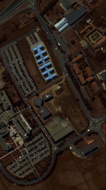
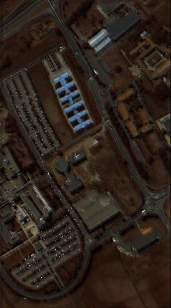
Pavia university is obtained by ROSIS-3 optical airborne sensor over the area of the University of Pavia, Italy. The HSI consists of pixels and has a spatial resolution of 1.3m. It has 115 bands, and 93 spectral bands are preserved after removing the spectral bands of low signal-noise-ratio (SNR). To simulate the low-resolution HSI, we apply an Gaussian blur kernel with a mean value of zero and a standard deviation of 3 to filter the reference image and then subsample the filtered image with factor 5. The four-band MSI is simulated by filtering the reference image with the IKONOS-like spectral response. The independent and identically distributed Gaussian noise is added to the simulated MSI (35dB) and simulated HSI (32dB).
4.3.2 Cuprite Mine
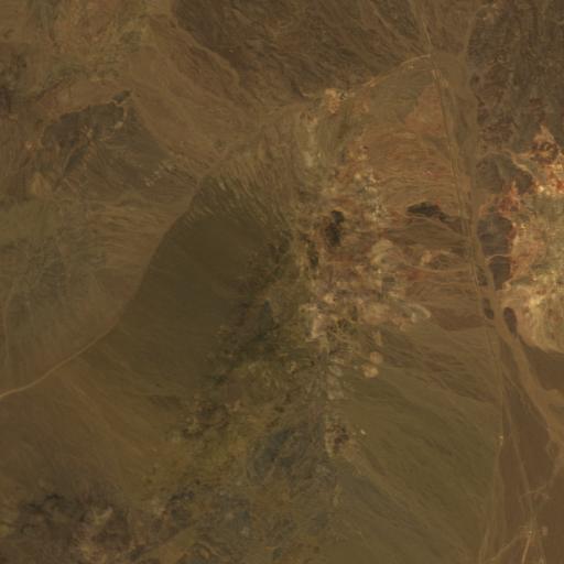
Cuprite Mine is obtained by the AVIRIS sensor over Cuprite mining district in Nevada in 1995. This image contains pixels, and top-left pixels are used for the experiments. The spatial resolution of this image is 17m. This image has 224 spectral bands, 188 spectral bands are preserved after removing the spectral bands of low signal-noise-ratio (SNR). To simulate the low-resolution HSI, we apply an Gaussian blur kernel with a mean value of zero and a standard deviation of 3 to filter the reference image and then subsample the filtered image with factor 4. Six-band high-resolution MSI is simulated by selecting wavelengths 480, 560, 660, 830, 1650, and 2220nm. The independent and identically distributed Gaussian noise is added to the simulated MSI (35dB) and simulated HSI (32dB).
4.4 Quantitative Evaluation
We further evaluate the quality fused HSI obtained by the testing approaches via quantitative indexes, consisting of PSNR, ERGAS, SAM, UIQI, and T. Tables 4 and 5 show the quantitative indexes on Cuprite Mine and Pavia University, respectively.
From two tables, the following observations can be obtained:
1) The pan-sharpening based HSI-MSI fusion methods, including GSA and GLP-HS, have a low computational burden and can be implemented much faster than other methods. However, the quality metrics of them are comparatively poor. The underlying reason is that they do not consider the observational model of the MSI and HSI, which is crucial for the fusion.
2) The MF based approaches, consisting of NSSR, CNMF, CSU, and Fuse-S, achieve good performance on the two datasets. Among these methods, Fuse-S achieves the best performance, which exploits spectral subspace representation and patch-based sparse prior. However, it is very time-consuming, the computational burden mainly comes from the patch-based dictionary learning and sparse coding. The CNMF can achieve
good performance and high computational efficiency among the MF based approaches.
3) In the TR based fusion methods, the CSTF and LTMR produce better quality indexes on Cuprite and Pavia University. It is because that the LTMR is based on spatial similarities of the fused HSI. The spatial resolution of Cuprite Mine is lower than that of Pavia University, and therefore that non-local spatial similarities are also weaker. In general, the TR based approaches are also comparatively time-consuming.
4) CNN-Fus is deep CNN based fusion approaches and achieves the best fusion results on most of the quality metrics for the two datasets. The advantages of this method mainly come from spectral subspace representation and CNN based coefficients estimation, in which the spectral subspace representation can well maintain the spectral characteristics of the HSI, and CNN is good at preserving the spatial structures of the image.
4.5 Visual Evaluation
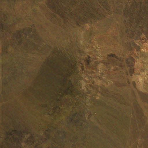
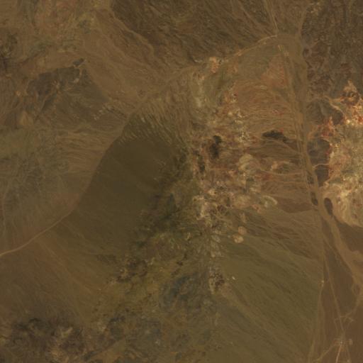
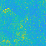
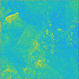
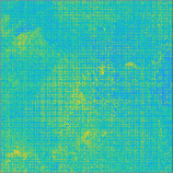
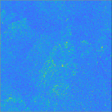
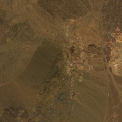
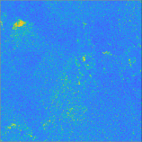
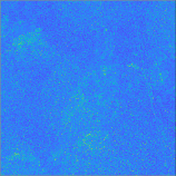
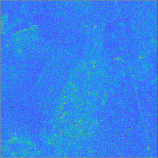
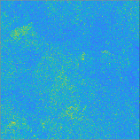
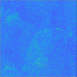
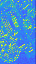
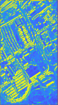
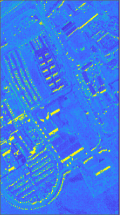
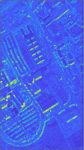
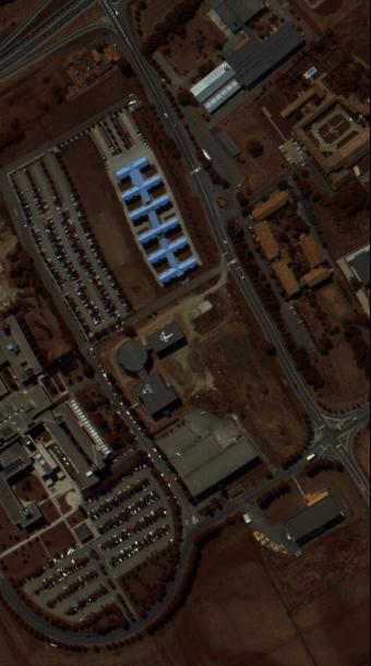
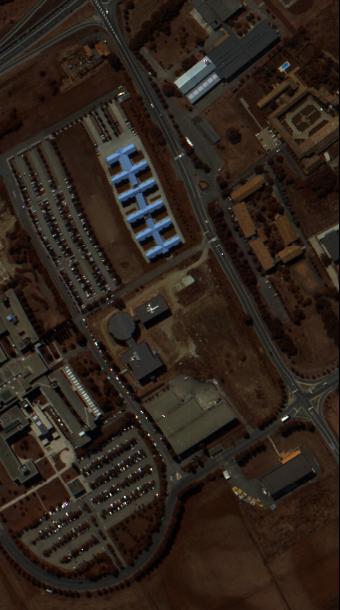
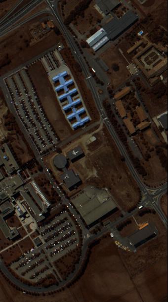
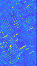
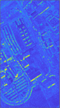
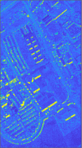
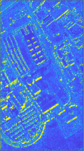
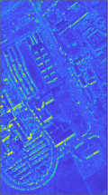
In addition to the quality metric evaluation, we also visually evaluate the fused images. Figure 2 shows false-color images formed by 30-th, 18-th, and 5-th bands and spectral error images of fused Cuprite Mine by testing methods, in which the spectral error image reflects the SAM for the fused HSI, and the false-color images mainly reflect the spatial structures of the fused HSI. As can be seen from Figure 2, the fused HSIs obtained by GSA, GLP-HS, and NSSR have severe spectral distortions, and the HSIs fused by CNMF, Fuse-S, CSTF, and CNN-Fus have much less spectral distortions. Figure 3 shows false-color images formed by 60-th, 29-th, and 7-th bands and spectral error images of fused Pavia University by testing methods. As can be seen from Figure 3, the HSIs fused by GSA and GLP-HS contain strong spectral errors. The fused HSIs obtained by Fuse-s and CNN-Fus have less spectral distortions. The advantages of the two methods mainly come from the spectral subspace representation, which can effectively model the spectral redundancies and similarities. The HSI fused by CSTF, CNMF, and CSU also contain relatively less spectral distortions, since they also make use of the low-rank prosperities of the spectral mode.
5 Challenges and New Guidelines for HSI-MSI fusion
HSI-MSI fusion has made significant progress in the past ten years. However, it remains some challenges. We present the existing challenges and new guidances for HSI-MSI fusion.
5.1 Image Registration
The image registration intends to geometrically align two images of the same scenario acquired by different sensors or at different times. Since HSI-MSI fusion requires that the MSI and HSI capture the image of the same scenario, and therefore image registration is a very crucial pre-processing step for HSI-MSI fusion. The image registration methods are categorized as area-based [97] and feature-based methods [98]. Although image registration approaches, such as scale-invariant Fourier transform [98], can produce most of the true matches, and it remains some false matches. However, most of the fusion methods assume that the HSI and MSI are perfectly aligned, and do not account for the distortions caused by the non-rigid registration. The fusion methods, which consider the non-rigid registration, will be a very important topic in future research. Since the deep CNN based methods solve the fusion problem in a supervised way, they may have superiority to reduce the distortions caused by non-rigid alignment.
5.2 HSI-MSI Fusion for Multi-temporal Images
The remote sensing HSI and MSI of the same scenario are often acquired at different time, which may result in different ground objects in the HSI and MSI. In this case, the HSI-MSI fusion is a very challenging problem, since the observation models for the HSI and MSI are hard to establish, and the image alignment is also tough. The existing fusion methods scarcely consider this challenging and meaningful problem, which needs to receive more attention. When applying the existing methods for the fusion of multi-temporal images, the fused image has obvious flaws and blur in the areas where the ground objects are changed. One possible way to solve the problem is to find the changed areas and giving less weight for the changed areas in the MSI.
5.3 HSI-MSI Fusion for Big Spatial Resolution Differences
In the Pan-sharpening, the spatial downsampling factor between PAN image and MSI factor is often 4. However, the spatial downsampling factor for HSI and MSI is often much higher than 4. For example, GF-2 can acquire MSI of 4m GSD, and GF-5 acquire MSI of 30m GSD. When the spatial resolutions of HSI and MSI have big differences, the essence of HSI-MSI fusion is solving a severely ill-posed problem, since most of the spatial information is lost. In this way, the fused HSI may contain severe spatial distortions. Therefore, the HSI-MSI fusion for big spatial resolution differences is a very challenging problem, and more efforts need to be made to solve this problem. The key to solving this problem is estimating the spatial degradation model accurately, which can reduce the spatial distortions.
5.4 The estimation of PSF and SRF
Many fusion methods, such as MF based methods and TR based ones, highly rely on the observation model (11), which assumes that the PSF and the SRF of the imaging sensor known. In the simulated data fusion, these methods can obtain satisfactory fusion results based on the perfectly-known PSF and SRF. However, they may not produce good fusion results in real data fusion, since the PSF and SRF may not be perfectly known in practice, and needs to be estimated in advance. Simões et al. [43] introduce an approach to estimate the PSF and SRF based on the following observation model
| (25) |
in which and denote the prior information on the and , respectively. They use the total variation to regularize the above two terms. However, they do not consider the non-negativity of the two terms and may obtain negative elements in and . What is more, the PSF can often be modeled as a Gaussian blur kernel, and this strong prior information may further contribute to the estimation of PSF.
5.5 Zero-short Learning for HSI-MSI Fusion
The deep learning based fusion methods often take an end-to-end way to learn the mapping from low-resolution HSI and high-resolution MSI to fused HSI. The deep learning based methods can achieve promising performance in terms of quality of fused HSI and computation efficacy. However, methods in this category mainly have two disadvantages when applying them to real data fusion. Firstly, they suffer from insufficient training data. In practice, the training data for HSI-MSI fusion is often not available. Furthermore, the well-trained deep CNN may have limited generalization ability, since the observational models, spectral range, and the number of spectral bands of the training data and testing data may be different. The possible way to solve the problem is zero-short learning, which trains the deep CNN from the data to be fused. In the training procedure, the training data is generated by spatially downsampling the observed HSI and MSI, and the observed HSI is used as the output of deep CNN. In this way, the spatial downsampling procedure for generating training data makes a difference, and the way of spatially downsampling procedure should be learned according to the spatial degeneration between the observed HSI and MSI.
5.6 Computation Efficiency
Since the grown size of HSI and MSI data, the computation efficiency is a very important index for the HSI. In remote sensing HSI-MSI fusion, the spatial size is often very large, and the number of spectral bands is usually over one hundred. Hence, the fusion approaches with the low computational cost are highly favored. The most of MF methods and TR methods suffer from high computational complexities since they need to iteratively solve the complex optimization problem. One available way to reduce the computational cost is low-dimensional subspace representation, which can significantly reduce the size of the spectral mode by exploiting the redundancies in the spectral mode. The other way is deep CNN based approaches, which take an end-to-end way to predict the fused HSI without iteration. What is more, they can be dramatically accelerated via the graphics processing unit (GPU).
6 Conclusions
This paper gives a comprehensive review for HSI-MSI fusion methods. In specific, we classify the approaches into four main families, i.e., pan-sharpening based methods, MF based methods, TR based methods, and deep CNN based methods, and we give detailed introductions and discussions for approaches in each category. What is more, we also analyze the existing challenges for HSI-MSI fusion and present the new guidances and potential research directions for HSI-MSI fusion.
Acknowledgement
This paper is supported by the Major Program of the National Natural Science Foundation of China (No. 61890962), the National Natural Science Foundation of China (No. 61801178), the Fund of Hunan Province for Science and Technology Plan Project under Grant (No. 2017RS3024), the Fund of Key Laboratory of Visual Perception and Artificial Intelligence of Hunan Province (No. 2018TP1013), and the Natural Science Foundation of Hunan Province (No. 2019JJ50036).
References
References
- [1] J. Bioucas-Dias, A. Plaza, G. Camps-Valls, P. Scheunders, N. Nasrabadi, J. Chanussot, Hyperspectral remote sensing data analysis and future challenges, IEEE Geosci. Remote Sens. Mag. 1 (2) (2013) 6–36.
- [2] Z. Pan, G. Healey, M. Prasad, B. Tromberg, Face recognition in hyperspectral images, IEEE Trans. Pattern Anal. Mach. Intell. 25 (12) (2003) 1552–1560. doi:10.1109/TPAMI.2003.1251148.
- [3] H. Akbari, Y. Kosugi, K. Kojima, N. Tanaka, Detection and analysis of the intestinal ischemia using visible and invisible hyperspectral imaging, IEEE Trans. Biomed. Eng. 57 (8) (2010) 2011–2017.
- [4] A. A. Goshtasby, S. Nikolov, Image fusion: Advances in the state of the art, Inf. Fus. 8 (2) (2007) 114–118.
- [5] S. Li, J. T. Kwok, Y. Wang, Using the discrete wavelet frame transform to merge Landsat TM and SPOT panchromatic images, Inf. Fus. 3 (1) (2002) 17–23.
- [6] J. J. Lewis, R. J. O. Callaghan, S. G. Nikolov, D. R. Bull, N. Canagarajah, Pixel- and region-based image fusion with complex wavelets, Inf. Fus. 8 (2) (2007) 119–130.
- [7] S. Yang, M. Wang, L. Jiao, R. Wu, Z. Wang, Image fusion based on a new Contourlet packet, Inf. Fus. 11 (2) (2010) 78–84.
- [8] Z. Liu, E. Blasch, V. John, Statistical comparison of image fusion algorithms: Recommendations, Inf. Fus. 36 (2017) 251–260.
-
[9]
Y. Liu, X. Chen, Z. Wang, Z. J. Wang, R. K. Ward, X. Wang,
Deep
learning for pixel-level image fusion: Recent advances and future prospects,
Information Fusion 42 (2018) 158 – 173.
doi:https://doi.org/10.1016/j.inffus.2017.10.007.
URL http://www.sciencedirect.com/science/article/pii/S1566253517305936 -
[10]
S. Li, X. Kang, L. Fang, J. Hu, H. Yin,
Pixel-level
image fusion: A survey of the state of the art, Information Fusion 33 (2017)
100 – 112.
doi:https://doi.org/10.1016/j.inffus.2016.05.004.
URL http://www.sciencedirect.com/science/article/pii/S1566253516300458 - [11] X. Liu, Q. Liu, Y. Wang, Remote sensing image fusion based on two-stream fusion network, Inf. Fus. 55 (2020) 1–15.
- [12] X. Meng, H. Shen, H. Li, L. Zhang, R. Fu, Review of the pansharpening methods for remote sensing images based on the idea of meta-analysis: Practical discussion and challenges, Inf. Fus. 46 (2019) 102–113.
- [13] L. Wang, B. Li, L. Tian, Multi-modal medical image fusion using the inter-scale and intra-scale dependencies between image shift-invariant Shearlet coefficients, Inf. Fus. 19 (1) (2014) 20–28.
- [14] L. G mez-Chova, D. Tuia, G. Moser, G. Camps-Valls, Multimodal classification of remote sensing images: A review and future directions, Proc. IEEE 103 (9) (2015) 1560–1584. doi:10.1109/JPROC.2015.2449668.
- [15] Y. Qu, H. Qi, B. Ayhan, C. Kwan, R. Kidd, Does multispectral/hyperspectral pansharpening improve the performance of anomaly detection?, in: IEEE Int. Geosci. Remote Sens. Symp., 2017, pp. 6130–6133. doi:10.1109/IGARSS.2017.8128408.
- [16] V. Ferraris, N. Dobigeon, Q. Wei, M. Chabert, Robust fusion of multiband images with different spatial and spectral resolutions for change detection, IEEE Trans. Comput. Imag. 3 (2) (2017) 175–186. doi:10.1109/TCI.2017.2692645.
- [17] G. Vivone, L. Alparone, J. Chanussot, M. Dalla Mura, A. Garzelli, G. A. Licciardi, R. Restaino, L. Wald, A critical comparison among pansharpening algorithms, IEEE Trans. Geosci. Remote Sens. 53 (5) (2015) 2565–2586.
- [18] L. Loncan, L. B. de Almeida, J. M. Bioucas-Dias, X. Briottet, J. Chanussot, N. Dobigeon, S. Fabre, W. Liao, G. A. Licciardi, M. Simões , J. Tourneret, M. A. Veganzones, G. Vivone, Q. Wei, N. Yokoya, Hyperspectral pansharpening: A review, IEEE Geosci. Remote Sens. Magaz. 3 (3) (2015) 27–46.
- [19] N. Yokoya, C. Grohnfeldt, J. Chanussot, Hyperspectral and multispectral data fusion: A comparative review of the recent literature, IEEE Geosci. Remote Sens. Mag. 5 (2) (2017) 29–56.
- [20] L. Tucker, Some mathematical notes on three-mode factor analysis, Psychometrika 23 (8) (1996) 3336–3351.
- [21] L.-J. Deng, M. Feng, X.-C. Tai, The fusion of panchromatic and multispectral remote sensing images via tensor-based sparse modeling and hyper-laplacian prior, Information Fusion 52 (2019) 76–89.
- [22] J. Ma, W. Yu, C. Chen, P. Liang, X. Guo, J. Jiang, Pan-gan: An unsupervised pan-sharpening method for remote sensing image fusion, Inf. Fus. 62 (2020) 110–120.
- [23] W. Carper, T. Lillesand, R. Kiefer, The use of intensity-hue-saturation transformations for merging spot panchromatic and multi-spectral image data, Photogramm. Eng. Remote Sens. 56 (4) (1990) 459–467.
- [24] P. S. Chavez, Jr., A. W. Kwarteng, Extracting spectral contrast in landsat thematic mapper image data using selective principal component analysis, Photogramm. Eng. Remote Sens. 55 (3) (1989) 339–348.
- [25] C. A. Laben, B. V. Brower, Process for enhancing the spatial resolution of multispectral imagery using pan-sharpening, U.S. Patent 6011875.
- [26] B. Aiazzi, S. Baronti, M. Selva, Improving component substitution pansharpening through multivariate regression of ms pan data, IEEE Trans. Geosci. Remote Sens. 45 (10) (2007) 3230–3239.
- [27] S. G. Mallat, A theory for multiresolution signal decomposition: the wavelet representation, IEEE Trans. Pattern Anal. Mach. Intell. 11 (7) (1989) 674–693.
- [28] M. J. Shensa, The discrete wavelet transform: wedding the a trous and mallat algorithms, IEEE Trans. Signal Process. 40 (10) (1992) 2464–2482.
- [29] P. Burt, E. Adelson, The laplacian pyramid as a compact image code, IEEE Trans. Commun. 31 (4) (1983) 532–540.
- [30] M. N. Do, M. Vetterli, The contourlet transform: an efficient directional multiresolution image representation, IEEE Trans. Image Process. 14 (12) (2005) 2091–2106.
- [31] J. Starck, J. Fadili, F. Murtagh, The undecimated wavelet decomposition and its reconstruction, IEEE Trans. Image Process. 16 (2) (2007) 297–309.
- [32] J. G. Liu, Comparison of three different methods to merge multiresolution and multispectral data: Landsat tm and spot panchromatic, Int. J. Remote Sens. 21 (18) (2000) 3461–3472.
- [33] P. S. C. Jr., S. C. Sides, J. A. Anderson, Comparison of three different methods to merge multiresolution and multispectral data: Landsat tm and spot panchromatic, Photogramm. Eng. Remote Sens. 57 (3) (1991) 295–303.
- [34] B. Aiazzi, L. Alparone, S. Baronti, A. Garzelli, M. Selva, Mtf-tailored multiscale fusion of high-resolution ms and pan imagery, Photogramm. Eng. Remote Sens. 72 (5) (2006) 591–596.
- [35] Z. Chen, H. Pu, B. Wang, G. Jiang, Fusion of hyperspectral and multispectral images: A novel framework based on generalization of pan-sharpening methods, IEEE Geosci. Remote Sens. Lett. 11 (8) (2014) 1418–1422.
- [36] M. Selva, B. Aiazzi, F. Butera, L. Chiarantini, S. Baronti, Hyper-sharpening: A first approach on sim-ga data, IEEE J. Sel. Top. Appl. Earth Observ. Remote Sens. 8 (6) (2015) 3008–3024.
- [37] R. Kawakami, J. Wright, Y.-W. Tai, Y. Matsushita, M. Ben-Ezra, K. Ikeuchi, High-resolution hyperspectral imaging via matrix factorization, IEEE CVPR (2011) 2329–2336.
- [38] B. Huang, H. Song, H. Cui, J. Peng, Z. Xu, Spatial and spectral image fusion using sparse matrix factorization, IEEE Trans. Geosci. Remote Sens. 52 (3) (2014) 1693–1704. doi:10.1109/TGRS.2013.2253612.
- [39] N. Akhtar, F. Shafait, A. Mian, Sparse spatio-spectral representation for hyperspectral image super-resolution, in: Euro. Conf. Comput. Vis., 2014, pp. 63 –78.
- [40] N. Akhtar, F. Shafait, A. Mian, Bayesian sparse representation for hyperspectral image super resolution, in: IEEE Conf. Comput. Vis. Pattern Recog., 2015, pp. 3631–3640.
- [41] Q. Wei, J. Bioucas-Dias, N. Dobigeon, J. Tourneret, Hyperspectral and multispectral image fusion based on a sparse representation, IEEE Trans. Geosci. Remote Sens. 53 (7) (2015) 3658–3668.
- [42] W. Dong, F. Fu, G. Shi, X. Cao, J. Wu, G. Li, X. Li, Hyperspectral image super-resolution via non-negative structured sparse representation, IEEE Trans. Image Process. 25 (5) (2016) 2337–2352.
- [43] M. Simões, J. Bioucas-Dias, L. Almeida, J. Chanussot, A convex formulation for hyperspectral image superresolution via subspace-based regularization, IEEE Trans. Geosci. Remote Sens. 53 (6) (2015) 3373–3388.
- [44] N. Yokoya, T. Yairi, A. Iwasaki, Coupled non-negative matrix factorization unmixing for hyperspectral and multispectral data fusion, IEEE Trans. Geosci. Remote Sens. 50 (2) (2012) 528–537.
- [45] C. Lanaras, E. Baltsavias, K. Schindler, Hyperspectral super-resolution by coupled spectral unmixing, in: IEEE Int. Conf. Comput. Vis., 2015, pp. 3586 –3594.
- [46] R. Dian, S. Li, L. Fang, Q. Wei, Multispectral and hyperspectral image fusion with spatial-spectral sparse representation, Inf. Fus. 49 (2019) 262–270.
- [47] Q. Wei, J. Bioucas-Dias, N. Dobigeon, J. Tourneret, M. Chen, S. Godsill, Multi-band image fusion based on spectral unmixing, IEEE Trans. Geosci. Remote Sens. 54 (12) (2016) 7236–7249.
- [48] M. Aharon, M. Elad, A. M. Bruckstein, K-SVD: An algorithm for designing of overcomplete dictionaries for sparse representations, IEEE Trans. Signal Process. 54 (11) (2006) 4311–4322.
- [49] J. Mairal, F. Bach, J. Ponce, G. Sapiro, Online dictionary learning for sparse coding, in: Int. Conf. Mach. Learn., 2009.
- [50] J. M. Nascimento, J. M. Dias, Vertex component analysis: A fast algorithm to unmix hyperspectral data, IEEE Trans. Geosci. Remote Sens. 43 (4) (2005) 898–910.
- [51] J. M. Bioucas-Dias, A variable splitting augmented lagrangian approach to linear spectral unmixing, in: Workshop on Hyperspectral Image and Signal Processing: Evolution in Remote Sensing, 2009, pp. 1–4.
- [52] X. Han, B. Shi, Y. Zheng, Self-similarity constrained sparse representation for hyperspectral image super-resolution, IEEE Trans. Image Process. 27 (11) (2018) 5625–5637. doi:10.1109/TIP.2018.2855418.
- [53] Y. Zhou, L. Feng, C. Hou, S. Kung, Hyperspectral and multispectral image fusion based on local low rank and coupled spectral unmixing, IEEE Trans. Geosci. Remote Sens. 55 (10) (2017) 5997–6009. doi:10.1109/TGRS.2017.2718728.
- [54] M. Veganzones, M. Simões, G. Licciardi, N. Yokoya, J. Bioucas-Dias, J. Chanussot, Hyperspectral super-resolution of locally low rank images from complementary multisource data, IEEE Trans. Geosci. Remote Sens. 25 (1) (2016) 274–288.
- [55] Q. Wei, N. Dobigeon, J. Tourneret, Fast fusion of multi-band images based on solving a Sylvester equation, IEEE Trans. Image Process. 24 (11) (2015) 4109–4121.
- [56] D. D. Lee, H. S. Seung, Learning the parts of objects by nonnegative matrix factorization, Nature 49 (6755) (1999) 788 C–791.
- [57] C. Lanaras, E. Baltsavias, K. Schindler, Hyperspectral super-resolution by coupled spectral unmixing, in: IEEE Int. Conf. Comput. Vis., 2015, pp. 3586 –3594.
- [58] S. Boyd, N. Parikh, E. Chu, B. Peleato, J. Eckstein, et al., Distributed optimization and statistical learning via the alternating direction method of multipliers, Found. Trends Mach. Learn. 3 (1) (2011) 1–122.
- [59] E. Wycoff, T. H. Chan, K. Jia, W. K. Ma, Y. Ma, A non-negative sparse promoting algorithm for high resolution hyperspecral imaging, IEEE ICASSP (2013) 1409–1413.
- [60] Y. Wu, H. Tan, Y. Li, J. Zhang, X. Chen, A fused CP factorization method for incomplete tensors, IEEE Trans. Neural Netw. Learn. Syst. 30 (3) (2019) 751–764.
- [61] Q. Zhao, G. Zhou, L. Zhang, A. Cichocki, S. Amari, Bayesian robust tensor factorization for incomplete multiway data, IEEE Trans. Neural Netw. Learn. Syst. 27 (4) (2016) 736–748. doi:10.1109/TNNLS.2015.2423694.
- [62] J. Chen, B. Jia, K. Zhang, Trifocal tensor-based adaptive visual trajectory tracking control of mobile robots, IEEE Trans. Cybern. 47 (11) (2017) 3784–3798. doi:10.1109/TCYB.2016.2582210.
- [63] B. Ma, L. Huang, J. Shen, L. Shao, Discriminative tracking using tensor pooling, IEEE Trans. Cybern. 46 (11) (2016) 2411–2422. doi:10.1109/TCYB.2015.2477879.
- [64] W. Wong, Z. Lai, Y. Xu, J. Wen, C. Ho, Joint tensor feature analysis for visual object recognition, IEEE Trans. Cybern. 45 (11) (2015) 2425–2436. doi:10.1109/TCYB.2014.2374452.
- [65] L. Feng, H. Sun, Q. Sun, G. Xia, Compressive sensing via nonlocal low-rank tensor regularization, Neurocomputing 216 (2016) 45–60.
- [66] Y. Peng, D. Meng, Z. Xu, C. Gao, Y. Yang, B. Zhang, Decomposable nonlocal tensor dictionary learning for multispectral image denoising, in: Proc. IEEE Int. Conf. Comput. Vis., 2014, pp. 2949–2956. doi:10.1109/CVPR.2014.377.
- [67] J. Xue, Y. Zhao, W. Liao, J. C. Chan, Nonlocal low-rank regularized tensor decomposition for hyperspectral image denoising, IEEE Trans. Geosci. Remote Sens. 57 (7) (2019) 5174–5189. doi:10.1109/TGRS.2019.2897316.
- [68] S. Yang, M. Wang, P. Li, L. Jin, B. Wu, L. Jiao, Compressive hyperspectral imaging via sparse tensor and nonlinear compressed sensing, IEEE Trans. Geosci. Remote Sens. 53 (11) (2015) 5943–5957. doi:10.1109/TGRS.2015.2429146.
- [69] J. Xue, Y. Zhao, W. Liao, J. Chan, Nonlocal tensor sparse representation and low-rank regularization for hyperspectral image compressive sensing reconstruction, Remote Sens. 11 (2).
- [70] R. Dian, L. Fang, S. Li, Hyperspectral image super-resolution via non-local sparse tensor factorization, in: IEEE Conf. Comput. Vis. Pattern Recog., 2017, pp. 5344–5353.
- [71] R. Dian, S. Li, L. Fang, T. Lu, J. M. Bioucas-Dias, Nonlocal sparse tensor factorization for semiblind hyperspectral and multispectral image fusion, IEEE Trans. Cyber.doi:10.1109/TCYB.2019.2951572.
- [72] S. Li, R. Dian, L. Fang, J. M. Bioucas-Dias, Fusing hyperspectral and multispectral images via coupled sparse tensor factorization, IEEE Trans. Image Process. 27 (8) (2018) 4118–4130. doi:10.1109/TIP.2018.2836307.
- [73] C. Pr vost, K. Usevich, P. Comon, D. Brie, Hyperspectral super-resolution with coupled Tucker approximation: Recoverability and SVD-based algorithms, IEEE Trans. Signal Process. 68 (2020) 931–946. doi:10.1109/TSP.2020.2965305.
- [74] Y. Chang, L. Yan, X. Zhao, H. Fang, Z. Zhang, S. Zhong, Weighted low-rank tensor recovery for hyperspectral image restoration, IEEE Trans Cyber. (2020) 1–15doi:10.1109/TCYB.2020.2983102.
- [75] C. I. Kanatsoulis, X. Fu, N. D. Sidiropoulos, W. Ma, Hyperspectral super-resolution: A coupled tensor factorization approach, IEEE Trans. Signal Process. 66 (24) (2018) 6503–6517. doi:10.1109/TSP.2018.2876362.
- [76] Y. Xu, Z. Wu, J. Chanussot, P. Comon, Z. Wei, Nonlocal coupled tensor cp decomposition for hyperspectral and multispectral image fusion, IEEE Trans. Geosci. Remote Sens 58 (1) (2020) 348–362. doi:10.1109/TGRS.2019.2936486.
- [77] M. E. Kilmer, K. Braman, N. Hao, R. C. Hoover, Third-order tensors as operators on matrices: A theoretical and computational framework with applications in imaging, SIAM J. Matrix Anal. Appl. 34 (1) (2013) 148–172.
- [78] I. Oseledets, Tensor-train decomposition, SIAM J. Sci. Comput. 33 (5) (2011) 2295–2317.
- [79] Y. Xu, Z. Wu, J. Chanussot, Z. Wei, Nonlocal patch tensor sparse representation for hyperspectral image super-resolution, IEEE Trans. Image Process. 28 (6) (2019) 3034–3047.
- [80] R. Dian, S. Li, Hyperspectral image super-resolution via subspace-based low tensor multi-rank regularization, IEEE Trans. Image Process. 28 (10) (2019) 5135–5146. doi:10.1109/TIP.2019.2916734.
- [81] R. Dian, S. Li, L. Fang, Learning a low tensor-train rank representation for hyperspectral image super-resolution, IEEE Trans. Neural Netw. Learn. Syst. 30 (9) (2019) 2672–2683. doi:10.1109/TNNLS.2018.2885616.
- [82] C. Dong, C. C. Loy, K. He, X. Tang, Learning a deep convolutional network for image super-resolution, in: Euro. conf. comput. vis., Springer, 2014, pp. 184–199.
- [83] C. Dong, C. C. Loy, K. He, X. Tang, Image super-resolution using deep convolutional networks, IEEE Trans. Pattern Anal. Mach. Intell. 38 (2) (2015) 295–307.
- [84] M. Giuseppe, C. Davide, V. Luisa, S. Giuseppe, Pansharpening by convolutional neural networks, Remote Sens. 8 (7) (2016) 594–.
- [85] J. Yang, X. Fu, Y. Hu, Y. Huang, X. Ding, J. Paisley, Pannet: A deep network architecture for pan-sharpening, in: IEEE Int. Conf. Comput. Vis., 2017, pp. 1753–1761.
- [86] R. Dian, S. Li, A. Guo, L. Fang, Deep hyperspectral image sharpening, IEEE Trans. Neural Netw. Learn. Syst. 29 (11) (2018) 5345–5355.
- [87] Q. Xie, M. Zhou, Q. Zhao, D. Meng, W. Zuo, Z. Xu, Multispectral and hyperspectral image fusion by ms/hs fusion net, in: IEEE Conf. Comput. Vis. Pattern Recog., 2019, pp. 1585–1594.
- [88] W. Xie, J. Lei, Y. Cui, Y. Li, Q. Du, Hyperspectral pansharpening with deep priors, IEEE Transactions on Neural Networks and Learning Systems (2019) 1–15.
- [89] R. Dian, S. Li, X. Kang, Regularizing hyperspectral and multispectral image fusion by cnn denoiser, IEEE Trans. Neural Netw. Learn. Syst. (2020) 1–12.
- [90] J. Yang, Y. Zhao, J. Chan, Hyperspectral and multispectral image fusion via deep two-branches convolutional neural network, Remote Sens. 10 (5) (2018) 800.
- [91] W. Wang, W. Zeng, Y. Huang, X. Ding, J. Paisley, Deep blind hyperspectral image fusion, in: IEEE Int. Conf. Comput. Vis., 2019, pp. 4149–4158.
- [92] X. Han, Y. Zheng, Y. Chen, Multi-level and multi-scale spatial and spectral fusion cnn for hyperspectral image super-resolution, in: IEEE Conf. Comput. Vis.n Workshop, 2019, pp. 4330–4339.
- [93] L. Wald, Quality of high resolution synthesised images: Is there a simple criterion?, in: Proc. Int. Conf. Fusion Earth Data, 2000, pp. 99 –103.
- [94] Z. Wang, A. Bovik, A universal image quality index, IEEE Signal Process. Lett. 9 (3) (2002) 81–84.
- [95] Z. Wang, A. Bovik, H. Sheikh, Image quality assessment: From error visibility to structural similarity, IEEE Trans. Image Process. 13 (4) (2004) 600–612.
- [96] F. Dell’Acqua, P. Gamba, A. Ferrari, J. Palmason, J. Benediktsson, K. Arnason, Exploiting spectral and spatial information in hyperspectral urban data with high resolution, IEEE Geosci. Remote Sens. Lett. 1 (4) (2004) 322–326. doi:10.1109/LGRS.2004.837009.
- [97] J. Le Moigne, W. J. Campbell, R. F. Cromp, An automated parallel image registration technique based on the correlation of wavelet features, IEEE Trans. Geosci. Remote Sens. 40 (8) (2002) 1849–1864.
- [98] D. Lowe, Distinctive image features from scale-invariant keypoints, Int. J. Comput. Vis. 60 (2) (2004) 91–110.