Grouping effects of sparse CCA models in variable selection

Abstract

The sparse canonical correlation analysis (SCCA) is a bi-multivariate association model that finds sparse linear combinations of two sets of variables that are maximally correlated with each other. In addition to the standard SCCA model, a simplified SCCA criterion which maixmizes the cross-covariance between a pair of canonical variables instead of their cross-correlation, is widely used in the literature due to its computational simplicity. However, the behaviors/properties of the solutions of these two models remain unknown in theory. In this paper, we analyze the grouping effect of the standard and simplified SCCA models in variable selection. In high-dimensional settings, the variables often form groups with high within-group correlation and low between-group correlation. Our theoretical analysis shows that for grouped variable selection, the simplified SCCA jointly selects or deselects a group of variables together, while the standard SCCA randomly selects a few dominant variables from each relevant group of correlated variables. Empirical results on synthetic data and real imaging genetics data verify the finding of our theoretical analysis.

I Introduction

Canonical correlation analysis (CCA) [1, 2] is a multivariate statistical method which investigates the associations between two sets of variables. It has found applications in statistics [3], data mining and machine learning [2, 4], functional magnetic resonance imaging [5, 6], genomics [7] and other fields [8]. Given two data sets $\mathbf{X}\in{}^{n\times p}$ and $\mathbf{Y}\in{}^{n\times q}$ measured on the same set of $n$ samples, CCA seeks linear combinations of the variables in $\mathbf{X}$ and those in $\mathbf{Y}$ that are maximally correlated with each other:

$$\underset{\mathbf{u},\mathbf{v}}{\text{maximize}}\;\mathbf{u}^{\rm T}\mathbf{X}^{\rm T}\mathbf{Y}\mathbf{v}\quad\text{s.t.}\quad\mathbf{u}^{\rm T}\mathbf{X}^{\rm T}\mathbf{X}\mathbf{u}\leq 1,\mathbf{v}^{\rm T}\mathbf{Y}^{\rm T}\mathbf{Y}\mathbf{v}\leq 1,$$

where $\mathbf{X}$ and $\mathbf{Y}$ are column-centered to zero mean.

Compared with multivariate multiple regression, the CCA is “symmetric” and more flexible in finding variables from both $\mathbf{X}$ and $\mathbf{Y}$ to predict each other well. However, in high dimensional setting ($n<p$) such as linking imaging to genomics [9, 10], the CCA breaks down because it has infinitely many solutions. In particular, the solution can have any support of cardinality greater than or equal to $n$, which means that the CCA can select an arbitrary set of $n$ or more variables. To handle that, the sparse CCA (SCCA) [11, 12, 13, 14, 15] utilizes the L1 sparsity regularization to select a subset of variables, which can improve the interpretability, stability as well as performance in variable selection.

A main drawback of the SCCA is that it is computationally expensive. To reduce the computational load, a common practice is to replace the covariance matrices $\mathbf{X}^{\rm T}\mathbf{X}$ and $\mathbf{Y}^{\rm T}\mathbf{Y}$ in the L2 constraints with diagonal matrices [16, 17, 18, 19, 20]. The resulting simplified SCCA model allows a closed-form solution for solving each subproblem (update of $\mathbf{u}$ with $\mathbf{v}$ fixed or vice versa) and is thus computationally more efficient.

However, the fundamental difference between the standard and simplified SCCA in variable selection remains unclear, particularly in the theoretical properties of their solutions. In [17, 20], the use of the simplified SCCA model is justified based only on the empirical observation that “in high-dimensional classification problems [21, 22], treating the covariance matrix as diagonal can yield good results”. In this paper, we attempt to close this gap by investigating the properties of the solutions of the standard and simplified SCCA models.

Our main contributions are summarized as follows.

• The behaviors of the standard and simplified SCCA models in grouped variable selection is theoretically characterized. In high-dimension small sample-size problems, the variables often form groups of various sizes with high within-group correlation and low between-group correlation. It shows that the simplified SCCA jointly selects or deselects a group of correlated variables together, while the standard SCCA tends to select a few dominant variables from each relevant group of correlated variables. This finding could be used by practitioners using SCCA, allowing them to select the proper method for their tasks.

• The Lemma 2.2 of [17] is extended from $c\in[\sqrt{|\mathcal{S}|},\infty)$ to $c\in(0,\infty)$, where ${\mathcal{S}}=\left\{i:i\in\operatorname*{argmax}_{j}\left|a_{j}\right|\right\}$. The Lemma 2.2 of [17], which solves $\underset{\mathbf{u}}{\text{maximize}}\;\mathbf{a}^{\rm T}\mathbf{u}$ subject to $\left\|\mathbf{u}\right\|^{2}\leq 1,\left\|\mathbf{u}\right\|_{1}\leq c$, is a key component of the simplified SCCA algorithm used to solve the subproblems at each iteration of the alternating optimization algorithm. However, the lemma fails to provide a solution to the above problem for $c\in(0,\sqrt{|\mathcal{S}|})$.

• Greedy algorithms to sequentially compute multiple canonical components for standard and simplified SCCA are derived and presented. To the best of our knowledge, these algorithms are new.

Notation: Scalars are denoted as italic letters, column vectors as boldface lowercase letters, and matrices as boldface capitals. The $j$-th column vector of a matrix $\mathbf{X}$ is denoted as $\mathbf{x}_{j}$. The superscript ^T stands for the transpose. The $\left\|\mathbf{u}\right\|$ and $\left\|\mathbf{u}\right\|_{1}$ denote the Euclidean norm and $\ell_{1}$ norm of a vector $\mathbf{u}$, respectively. The $\sigma_{\rm max}\left(\mathbf{A}\right)$ and $\lambda_{\rm max}\left(\mathbf{A}\right)$ denote the largest singular value and largest eigenvalue of a matrix $\mathbf{A}$, respectively. For a set ${\mathcal{S}}$, its cardinality is denoted as $\left|{\mathcal{S}}\right|$. The soft-thresholding operator is defined as

$$\mathop{{\rm S}}\left(a,\Delta\right)=\begin{cases}a-\Delta,&a>\Delta\\ a+\Delta,&a<-\Delta\\ 0,&-\Delta\leq a\leq\Delta,\end{cases}$$

where $\Delta$ is a non-negative constant.

II Sparse CCA model

Assume that $\mathbf{X}$ and $\mathbf{Y}$ are column-centered to zero mean. SCCA aims to find a linear combination of variables in $\mathbf{X}$ and $\mathbf{Y}$ to maximize their correlation [15, 13]:

$$\underset{\mathbf{u},\mathbf{v}}{\text{maximize}} \mathbf{u}^{\rm T}\mathbf{X}^{\rm T}\mathbf{Y}\mathbf{v}$$ (1)

subject to $$\mathbf{u}^{\rm T}\mathbf{X}^{\rm T}\mathbf{X}\mathbf{u}\leq 1,\left\|\mathbf{u}\right\|_{1}\leq c_{1}$$

$$\mathbf{v}^{\rm T}\mathbf{Y}^{\rm T}\mathbf{Y}\mathbf{v}\leq 1,\left\|\mathbf{v}\right\|_{1}\leq c_{2},$$

where $\mathbf{X}\mathbf{u}$ and $\mathbf{Y}\mathbf{v}$ are the canonical variables, $\mathbf{u}$ and $\mathbf{v}$ are canonical loadings/weights measuring the contribution of each feature in the identified association, and $c_{1}>0,c_{2}>0$ are the regularization parameters that control the sparsity of the solution.

The problem (1) is not convenient to solve due to the quadratic constraints. To save the computational cost, it is a common practice to treat the covariance matrices $\mathbf{X}^{\rm T}\mathbf{X}$ and $\mathbf{Y}^{\rm T}\mathbf{Y}$ as diagonal [16, 17, 18, 19, 20, 14, 23]. This yields the following simplified formulation of SCCA:

$$\underset{\mathbf{u},\mathbf{v}}{\text{maximize}} \mathbf{u}^{\rm T}\mathbf{X}^{\rm T}\mathbf{Y}\mathbf{v}$$ (2)

subject to $$\left\|\mathbf{u}\right\|^{2}\leq 1,\left\|\mathbf{u}\right\|_{1}\leq c_{1}$$

$$\left\|\mathbf{v}\right\|^{2}\leq 1,\left\|\mathbf{v}\right\|_{1}\leq c_{2},$$

where $c_{1},c_{2}>0$.

In Section IV-B and Supplementary Materials Section C, we will describe algorithms to fit the two models, as well as explain how to obtain multiple canonical components.

III Grouping effect analysis

In high-dimensional problems such as imaging genomics, grouped variables are common and how to properly select them is an important research problem [10, 24, 25, 26]. For a sparse CCA model, we say it exhibits the grouping effect if it jointly selects or deselects each group of highly correlated variables together.

To gain initial insights, we start with the simplest case with all $p$ $X$ variables fully correlated with each other.

Lemma III.1.

Let $\mathbf{x}_{1}=\mathbf{x}_{2}=\dots=\mathbf{x}_{p}$ have unit L2 norm.

The optimal solution $\mathbf{u}^{*}$ to problem (1) is

(i)

any point on the segment of the line $u_{1}+u_{2}+\dots+u_{p}=1$ that is inside the L1 ball:

$${\color[rgb]{0,0,0}{{u_{1}^{*}+u_{2}^{*}+\dots+u_{p}^{*}}}} =1$$ (3)

$$\left\|\mathbf{u}^{*}\right\|_{1} \leq c_{1}$$ (4)

when $c_{1}\geq 1$, and

(ii)

any $u_{1}^{*}\geq 0,u_{2}^{*}\geq 0,\dots,u_{p}^{*}\geq 0$ that satisfy:

$${\color[rgb]{0,0,0}{{u_{1}^{*}+u_{2}^{*}+\dots+u_{p}^{*}}}}=c_{1}$$ (5)

when $0<c_{1}<1$.

The optimal solution $\mathbf{u}^{*}$ to problem (2) is:

(i)

${\color[rgb]{0,0,0}{{u_{1}^{*}=u_{2}^{*}=\dots=u_{p}^{*}}}}=\frac{1}{\sqrt{p}}$ when $c_{1}\geq\sqrt{p}$, and

(ii)

any $u_{1}^{*}\geq 0,u_{2}^{*}\geq 0,\dots,u_{p}^{*}\geq 0$ that satisfy:

$${\color[rgb]{0,0,0}{{u_{1}^{*}+u_{2}^{*}+\dots+u_{p}^{*}}}} =c_{1}$$ (6)

$${\color[rgb]{0,0,0}{{{u_{1}^{*}}^{2}}}}+{u_{2}^{*}}^{2}+\dots+{u_{p}^{*}}^{2} \leq 1$$ (7)

when $1\leq c_{1}<\sqrt{p}$.

Proof.

We first prove the result for problem (1), i.e., the SCCA model.

When $\mathbf{x}_{1}=\mathbf{x}_{2}=\dots=\mathbf{x}_{p}\triangleq\mathbf{x}$, the problem (1) reduces to

$$\underset{\mathbf{u},\mathbf{v}}{\text{maximize}} (u_{1}+u_{2}+\dots+u_{p})\mathbf{x}^{\rm T}\mathbf{Y}\mathbf{v}$$ (8)

subject to $$\left|u_{1}+u_{2}+\dots+u_{p}\right|\leq 1,\left\|\mathbf{u}\right\|_{1}\leq c_{1}$$

$$\mathbf{v}^{\rm T}\mathbf{Y}^{\rm T}\mathbf{Y}\mathbf{v}\leq 1,\left\|\mathbf{v}\right\|_{1}\leq c_{2},$$

where $c_{1}\geq 1$, $c_{2}\geq 1$.

Note that the optimal solution to problem (8) is not unique because the objective function remains the same after we reverse the signs of both $\mathbf{u}$ and $\mathbf{v}$. To resolve this, we assume $u_{1}+u_{2}+\dots+u_{p}\geq 0$.

Note also that the optimal value of problem (8) is larger than zero when $c_{1}>0,c_{2}>0$.

As a result, $\mathbf{u}$ and $\mathbf{v}$ can be independently optimized:

$$\begin{aligned} \mathbf{u}^{*}&=\underset{\mathbf{u}}{\operatorname*{argmax}}&&(u_{1}+u_{2}+\dots+u_{p})\\ &\text{subject to}&&\left|u_{1}+u_{2}+\dots+u_{p}\right|\leq 1,\left\|\mathbf{u}\right\|_{1}\leq c_{1}\\ \end{aligned}$$ (9)

$$\begin{aligned} \mathbf{v}^{*}&=\underset{\mathbf{v}}{\operatorname*{argmax}}&&\mathbf{x}^{\rm T}\mathbf{Y}\mathbf{v}\\ &\text{subject to}&&\mathbf{v}^{\rm T}\mathbf{Y}^{\rm T}\mathbf{Y}\mathbf{v}\leq 1,\left\|\mathbf{v}\right\|_{1}\leq c_{2}.\end{aligned}$$ (10)

Solving (9) yields the optimal solution $\mathbf{u}^{*}$ shown in (3)-(5).

We next prove the result regarding problem (2), i.e., the simplified SCCA model.

When $\mathbf{x}_{1}=\mathbf{x}_{2}=\dots=\mathbf{x}_{p}\triangleq\mathbf{x}$, the problem (2) reduces to

$$\underset{\mathbf{u},\mathbf{v}}{\text{maximize}} (u_{1}+u_{2}+\dots+u_{p})\mathbf{x}^{\rm T}\mathbf{Y}\mathbf{v}$$ (11)

subject to $$\left\|\mathbf{u}\right\|^{2}\leq 1,\left\|\mathbf{u}\right\|_{1}\leq c_{1}$$

$$\left\|\mathbf{v}\right\|^{2}\leq 1,\left\|\mathbf{v}\right\|_{1}\leq c_{2},$$

where $c_{1}\geq 1$, $c_{2}\geq 1$.

To resolve sign ambiguity, we assume $u_{1}+u_{2}+\dots+u_{p}\geq 0$. Therefore, $\mathbf{u}$ and $\mathbf{v}$ can be independently optimized:

$$\mathbf{u}^{*} =\underset{\mathbf{u}}{\operatorname*{argmax}} (u_{1}+u_{2}+\dots+u_{p})$$ (12)

subject to $$\left\|\mathbf{u}\right\|^{2}\leq 1,\left\|\mathbf{u}\right\|_{1}\leq c_{1}$$

$$\mathbf{v}^{*} =\underset{\mathbf{v}}{\operatorname*{argmax}} \mathbf{x}^{\rm T}\mathbf{Y}\mathbf{v}$$ (13)

subject to $$\left\|\mathbf{v}\right\|^{2}\leq 1,\left\|\mathbf{v}\right\|_{1}\leq c_{2}.$$

Solving (12) yields the optimal solution shown in Lemma III.1 (simplified SCCA part). ∎

We then provide a formal proof of the grouping effects in variable selection for the simplified SCCA.

Theorem III.2.

Given data $\left(\mathbf{X},\mathbf{Y}\right)$, with columns standardized to zero mean and unit norm, and regularization parameters $\left(c_{1},c_{2}\right)$. Let $\left(\mathbf{u}^{*},\mathbf{v}^{*}\right)$ be an optimal solution to problem (2). Assume at $\left(\mathbf{u}^{*},\mathbf{v}^{*}\right)$ the L2 inequality constraint on $\mathbf{u}$ is strongly active. We have:

• when $u_{i}^{*}u_{j}^{*}>0$

  $$\left|u_{i}^{*}-u_{j}^{*}\right|$$ (14)

  $$\leq\; \frac{1}{\alpha_{1}}\mathop{{\rm min}}\left({\color[rgb]{0,0,0}{{\sigma_{\rm max}}}}\left(\mathbf{Y}\right),c_{2}\sqrt{\sum_{\ell=1}^{n}\max_{1\leq j\leq q}y_{\ell j}^{2}}\right)\sqrt{\left(1-r_{ij}\right)/2}$$

• when $u_{i}^{*}u_{j}^{*}<0$

  $$\left|u_{i}^{*}+u_{j}^{*}\right|$$ (15)

  $$\leq\; \frac{1}{\alpha_{1}}\mathop{{\rm min}}\left({\color[rgb]{0,0,0}{{\sigma_{\rm max}}}}\left(\mathbf{Y}\right),c_{2}\sqrt{\sum_{\ell=1}^{n}\max_{1\leq j\leq q}y_{\ell j}^{2}}\right)\sqrt{\left(1+r_{ij}\right)/2},$$

where $r_{ij}=\mathbf{x}_{i}^{\rm T}\mathbf{x}_{j}\in[-1,1]$ is the Pearson correlation coefficient between $\mathbf{x}_{i}$ and $\mathbf{x}_{j}$, and $\alpha_{1}>0$ is a constant that only depends on $\left(\mathbf{X},\mathbf{Y},c_{1},c_{2}\right)$.

Likewise, if at $\left(\mathbf{u}^{*},\mathbf{v}^{*}\right)$ the L2 inequality constraint on $\mathbf{v}$ is strongly active, we have

• when $v_{i}^{*}v_{j}^{*}>0$

  $$\left|v_{i}^{*}-v_{j}^{*}\right|$$ (16)

  $$\leq\; \frac{1}{\alpha_{2}}\mathop{{\rm min}}\left({\color[rgb]{0,0,0}{{\sigma_{\rm max}}}}\left(\mathbf{X}\right),c_{1}\sqrt{\sum_{\ell=1}^{n}\max_{1\leq i\leq p}x_{\ell i}^{2}}\right)\sqrt{(1-r_{ij}^{\prime})/2}$$

• when $v_{i}^{*}v_{j}^{*}<0$

  $$\left|v_{i}^{*}+v_{j}^{*}\right|$$ (17)

  $$\leq\; \frac{1}{\alpha_{2}}\mathop{{\rm min}}\left({\color[rgb]{0,0,0}{{\sigma_{\rm max}}}}\left(\mathbf{X}\right),c_{1}\sqrt{\sum_{\ell=1}^{n}\max_{1\leq i\leq p}x_{\ell i}^{2}}\right)\sqrt{\left(1+r_{ij}^{\prime}\right)/2},$$

where $r_{ij}^{\prime}=\mathbf{y}_{i}^{\rm T}\mathbf{y}_{j}\in[-1,1]$ is the Pearson correlation coefficient between $\mathbf{y}_{i}$ and $\mathbf{y}_{j}$, and $\alpha_{2}>0$ is a constant that only depends on $\left(\mathbf{X},\mathbf{Y},c_{1},c_{2}\right)$.

Proof.

Since each subproblem (solve for $\mathbf{u}$ with $\mathbf{v}$ fixed or solve for $\mathbf{v}$ with $\mathbf{u}$ fixed) is a convex optimization problem with differentiable objective and constraint functions (The L1 inequality constraint can be written as $2^{p}$ linear inequality constraints), and is strictly feasible (Slater’s condition holds), the KKT conditions provide necessary and sufficient conditions for optimality [27].

The KKT conditions for the optimality of $\mathbf{u}^{*}$ consist of the following conditions:

$$2\alpha_{1}\mathbf{u}^{*}+\lambda_{1}\mathbf{s}=\mathbf{X}^{\rm T}\mathbf{Y}\mathbf{v}^{*},$$ (18)

where $s_{i}=\mathop{{\rm sign}}\left(u_{i}^{*}\right)$ if $u_{i}^{*}\neq 0$; otherwise, $s_{i}\in[-1,1]$.

$$\alpha_{1}\geq 0,\quad\left\|\mathbf{u}^{*}\right\|^{2}\leq 1,\quad\alpha_{1}\left(\left\|\mathbf{u}^{*}\right\|^{2}-1\right)=0$$ (19)

$$\lambda_{1}\geq 0,\quad\left\|\mathbf{u}^{*}\right\|_{1}\leq c_{1},\quad\lambda_{1}\left(\left\|\mathbf{u}^{*}\right\|_{1}-c_{1}\right)=0.$$ (20)

If $u_{i}^{*}u_{j}^{*}>0$, then both $u_{i}^{*}$ and $u_{j}^{*}$ are non-zero with $\mathop{{\rm sign}}\left(u_{i}^{*}\right)=\mathop{{\rm sign}}\left(u_{j}^{*}\right)$. From (18), it follows that

$$2\alpha_{1}u_{i}^{*}+\lambda_{1}\mathop{{\rm sign}}\left(u_{i}^{*}\right) =\mathbf{x}_{i}^{\rm T}\mathbf{Y}\mathbf{v}^{*}$$ (21)

$$2\alpha_{1}u_{j}^{*}+\lambda_{1}\mathop{{\rm sign}}\left(u_{j}^{*}\right) =\mathbf{x}_{j}^{\rm T}\mathbf{Y}\mathbf{v}^{*}.$$ (22)

Subtracting (22) from (21) gives

$$2\alpha_{1}\left(u_{i}^{*}-u_{j}^{*}\right)=\left(\mathbf{x}_{i}-\mathbf{x}_{j}\right)^{\rm T}\mathbf{Y}\mathbf{v}^{*}.$$ (23)

Therefore, we have

$$\left|u_{i}^{*}-u_{j}^{*}\right| =\frac{1}{2\alpha_{1}}\left|\left(\mathbf{x}_{i}-\mathbf{x}_{j}\right)^{\rm T}\mathbf{Y}\mathbf{v}^{*}\right|$$ (24)

$$\leq\frac{1}{2\alpha_{1}}\left\|\mathbf{x}_{i}-\mathbf{x}_{j}\right\|\left\|\mathbf{Y}\mathbf{v}^{*}\right\|.$$

Since $\mathbf{X}$ is column standardized, we have

$$\left\|\mathbf{x}_{i}-\mathbf{x}_{j}\right\|=\sqrt{\left\|\mathbf{x}_{i}\right\|^{2}+\left\|\mathbf{x}_{j}\right\|^{2}-2\mathbf{x}_{i}^{\rm T}\mathbf{x}_{j}}=\sqrt{2\left(1-r_{ij}\right)},$$ (25)

where $r_{ij}=\mathbf{x}_{i}^{\rm T}\mathbf{x}_{j}$ is the sample Pearson correlation coefficient between $\mathbf{x}_{i}$ and $\mathbf{x}_{j}$.

In the domain of problem (2), it holds that

$$\left\|\mathbf{Y}\mathbf{v}^{*}\right\|\leq\sigma_{\rm max}\left(\mathbf{Y}\right)\left\|\mathbf{v}^{*}\right\|\leq\sigma_{\rm max}\left(\mathbf{Y}\right)$$ (26)

and

$$\left\|\mathbf{Y}\mathbf{v}^{*}\right\| =\sqrt{\sum_{\ell=1}^{n}\left(\sum_{j=1}^{q}y_{\ell j}v_{j}^{*}\right)^{2}}$$ (27)

$$\leq \sqrt{\sum_{\ell=1}^{n}\max_{1\leq j\leq q}y_{\ell j}^{2}\left(\sum_{j=1}^{q}\left|v_{j}^{*}\right|\right)^{2}}$$

$$= \sqrt{\sum_{\ell=1}^{n}\max_{1\leq j\leq q}y_{\ell j}^{2}}\left\|\mathbf{v}^{*}\right\|_{1}$$

$$\leq c_{2}\sqrt{\sum_{\ell=1}^{n}\max_{1\leq j\leq q}y_{\ell j}^{2}},$$

where in (26) and (27) we have used the L2 and L1 constraints in problem (2), respectively.

Substituting (25)-(27) into (24), we arrive at

$$\left|u_{i}^{*}-u_{j}^{*}\right|$$

$$\leq\; \frac{1}{\alpha_{1}}\mathop{{\rm min}}\left(\sigma_{\rm max}\left(\mathbf{Y}\right),c_{2}\sqrt{\sum_{\ell=1}^{n}\max_{1\leq j\leq q}y_{\ell j}^{2}}\right)\sqrt{\left(1-r_{ij}\right)/2}.$$ (28)

Since the L2 inequality constraint on $\mathbf{u}$ is strongly active at $\left(\mathbf{u}^{*},\mathbf{v}^{*}\right)$, we have $\alpha_{1}>0$. Specifically, combining conditions (18)-(20) yields

$$\alpha_{1}=\frac{1}{2}\left\|{\color[rgb]{0,0,0}{{\mathop{{\rm S}}\left(\mathbf{X}^{\rm T}\mathbf{Y}\mathbf{v}^{*},\lambda_{1}\right)}}}\right\|,$$ (29)

where $\lambda_{1}=0$ if this results in $\frac{\left\|\mathbf{X}^{\rm T}\mathbf{Y}\mathbf{v}^{*}\right\|_{1}}{\left\|\mathbf{X}^{\rm T}\mathbf{Y}\mathbf{v}^{*}\right\|}\leq c_{1}$; otherwise, $\lambda_{1}$ is the smallest positive number for which it satisfies $\frac{\left\|{\color[rgb]{0,0,0}{{\mathop{{\rm S}}\left(\mathbf{X}^{\rm T}\mathbf{Y}\mathbf{v}^{*},\lambda_{1}\right)}}}\right\|_{1}}{\left\|{\color[rgb]{0,0,0}{{\mathop{{\rm S}}\left(\mathbf{X}^{\rm T}\mathbf{Y}\mathbf{v}^{*},\lambda_{1}\right)}}}\right\|}=c_{1}$. Thus we obtain (14).

Using a similar line of argumentation, we can prove (15) and (16)-(17). ∎

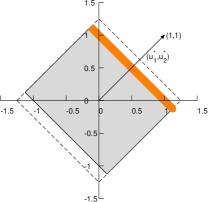
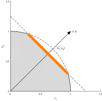
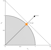
Figure 1: The optimal solution set $\mathbf{u}^{*}$ with $p=2$ identical variables. (a) the SCCA problem with $c_{1}=1.25$; (b) simplified SCCA with $c_{1}=1.25$; (c) simplified SCCA with $c_{1}=1.5$. The feasible set of points are shown lightly shaded. The optimal points are highlighted in orange.

Fig. 1 illustrates the optimal solution $\mathbf{u}^{*}$ to problems (1) and (2) with $p=2$ identical $X$ variables. We see that for SCCA (Fig. S1), the optimal solution set is a line segment that cross the axes (i.e., includes sparse solutions). While for simplified SCCA (Figs. S1-1), the optimal solution set does not intersect with the axes (i.e., does not include sparse or nearly sparse solutions); in particular, when the L2 constraint on $\mathbf{u}$ is strongly active at the optimal solution, i.e., when $c_{1}\geq\sqrt{2}$, the optimal solution set contains a single point with equal coordinates: $(u_{1}^{*},u_{2}^{*})=\left(\frac{\sqrt{2}}{2},\frac{\sqrt{2}}{2}\right)$.

IV Optimization Algorithms

Both problems (1) and (2) are bi-convex, i.e., convex in $\mathbf{u}$ with $\mathbf{v}$ fixed and in $\mathbf{v}$ with $\mathbf{u}$ fixed, but not jointly convex in $\mathbf{u}$ and $\mathbf{v}$. A standard method to solve the SCCA models is alternating optimization [28]: it first updates $\mathbf{u}$ while holding $\mathbf{v}$ fixed and then updates $\mathbf{v}$ while holding $\mathbf{u}$ fixed, and repeats this process until convergence.

IV-A SCCA model (1)

The SCCA model fitting algorithm is shown in Algorithm 1.

Algorithm 1 SCCA algorithm

1:  Initialize $\mathbf{v}$;

2:  repeat

3:     Update $\mathbf{u}$ with $\mathbf{v}$ fixed:

$$\underset{\mathbf{u}}{\text{maximize}} \mathbf{u}^{\rm T}\mathbf{X}^{\rm T}\mathbf{Y}\mathbf{v}$$ (30)

subject to $$\left\|\mathbf{X}\mathbf{u}\right\|^{2}\leq 1,\left\|\mathbf{u}\right\|_{1}\leq c_{1}$$

4:     Update $\mathbf{v}$ with $\mathbf{u}$ fixed:;

$$\underset{\mathbf{v}}{\text{maximize}} \mathbf{u}^{\rm T}\mathbf{X}^{\rm T}\mathbf{Y}\mathbf{v}$$ (31)

subject to $$\mathbf{v}^{\rm T}\mathbf{Y}^{\rm T}\mathbf{Y}\mathbf{v}\leq 1,\left\|\mathbf{v}\right\|_{1}\leq c_{2}$$

5:  until convergence.

Both problems (30) and (31) are convex optimization problems, and in [15] the linearized alternating direction method of multipliers (ADMM) [29] algorithm has been proposed to solve each of them. Since in [15] it uses a slightly different formulation (therein the L1 regularizer appears in the objective function), we have presented a new linearized ADMM algorithm to solve problem (30) in Supplementary Materials A.

IV-B Simplified SCCA model (2)

We first introduce the following lemma, which will be used as a building block in the simplified SCCA algorithm.

Lemma IV.1.

Consider the quadratically constrained linear program (QCLP) optimization problem:

$$\underset{\mathbf{u}}{\text{maximize}}\;\mathbf{a}^{\rm T}\mathbf{u}\quad\text{subject to }\left\|\mathbf{u}\right\|^{2}\leq 1,\left\|\mathbf{u}\right\|_{1}\leq c,$$ (32)

where $c>0$ is a constant.

Define ${\mathcal{S}}=\left\{i:i\in\operatorname*{argmax}_{j}\left|a_{j}\right|\right\}$. The optimal solution $\mathbf{u}^{*}$ to (32) is as below.

• Case 1 : $c<\sqrt{\left|{\mathcal{S}}\right|}$

  $$[\mathbf{u}^{*}]_{i}=\begin{cases}\frac{c}{\left|{\mathcal{S}}\right|}\mathop{{\rm sign}}\left(a_{i}\right),&i\in{\mathcal{S}}\\ 0,&i\notin{\mathcal{S}}\end{cases}$$ (33)

• Case 2: $c\geq\sqrt{\left|{\mathcal{S}}\right|}$

  $$\mathbf{u}^{*}=\frac{{\color[rgb]{0,0,0}{{\mathop{{\rm S}}\left(\mathbf{a},\Delta\right)}}}}{\left\|{\color[rgb]{0,0,0}{{\mathop{{\rm S}}\left(\mathbf{a},\Delta\right)}}}\right\|}$$ (34)

  where $\Delta=0$ if this results $\left\|\mathbf{u}^{*}\right\|_{1}\leq c$; otherwise, $\Delta>0$ satisfies $\left\|\mathbf{u}^{*}\right\|_{1}=c$. Here the soft-thresholding ${\color[rgb]{0,0,0}{{\mathop{{\rm S}}\left(\mathbf{a},\Delta\right)}}}$ is applied to $\mathbf{a}$ coordinate-wise.

The above lemma extends Lemma 2.2 of [17] from $c\in[\sqrt{\left|{\mathcal{S}}\right|},\infty)$ to $c\in(0,\infty)$. See Supplementary Materials Section B for the proof of Lemma IV.1 and how it extends Lemma 2.2 of [17].

For the simplified SCCA in (2), each subproblem (solving $\mathbf{u}$ with $\mathbf{v}$ fixed or solving $\mathbf{v}$ with $\mathbf{u}$ fixed) is a QCLP problem of form (32), which results in Algorithm 2.

Algorithm 2 Simplified SCCA algorithm

1:  Initialize $\mathbf{v}$;

2:  repeat

3:     Update $\mathbf{u}$ according to Lemma IV.1, with $\mathbf{a}=\mathbf{X}^{\rm T}\mathbf{Y}\mathbf{v}$ and $c=c_{1}$;

4:     Update $\mathbf{v}$ according to Lemma IV.1, with $\mathbf{a}=\mathbf{Y}^{\rm T}\mathbf{X}\mathbf{u}$ and $c=c_{2}$;

5:  until convergence.

Note that by repeatedly applying Algorithms 1 and 2, we can obtain multiple canonical components, as described in Section C in Supplemental Materials.

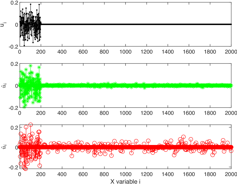
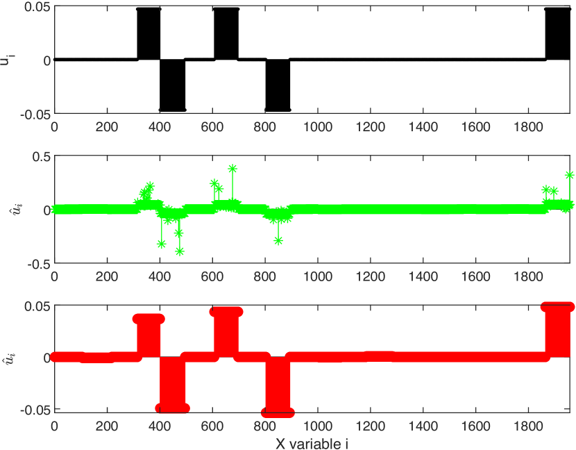
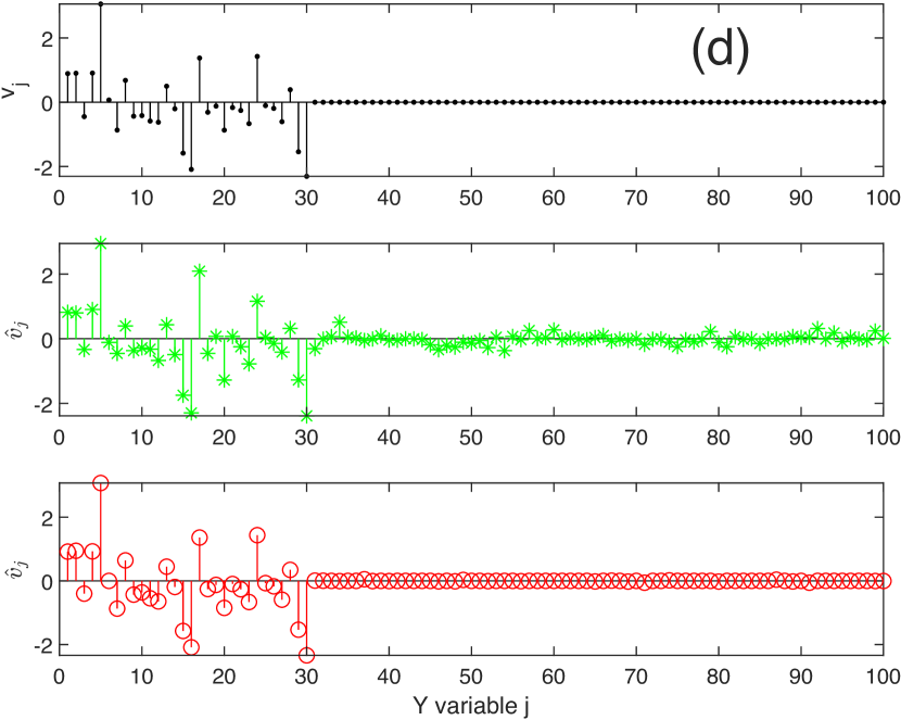
Figure 2: The actual and estimated canonical weight vectors $\mathbf{u}$ and $\mathbf{v}$ for (a-b) Experiment 1 and (c-d) Experiment 2. In each subfigure, the top row shows the actual weights used in the generative model, and the bottom two rows show the weights estimated by SCCA and simplified SCCA on all training data, respectively. To facilitate comparison, the estimated weight vectors are scaled to have the same Euclidean norm as the actual weight vector.

V Experimental results and discussion

We perform comparative study of the two SCCA models using both synthetic data and real imaging genetics data.

V-A Simulation study on synthetic data

Assume the data $\mathbf{X}\in{}^{n\times p}$ and $\mathbf{Y}\in{}^{n\times q}$ collect $n$ i.i.d. observations/samples of random vectors $\mathbf{x}\in{}^{p\times 1}$ and $Y\in{}^{q\times 1}$ (with slight abuse of notation), respectively, with $n=1000,p\approx 2000,q=100$. We consider two simulation setups, one with uncorrelated variables and the other with grouped variables. For simplicity, we focus on the simulation and analysis of $X$ variables only.

TABLE I: Performance comparison on canonical correlation coefficients on synthetic data.

		Training				Testing
Model	$\left(c_{1}^{\rm opt},c_{2}^{\rm opt}\right)$	Cov@Val∗	Corr@Val∗	Cov∗∗	Corr∗∗	Cov	Corr
Experimental setup 1
SCCA	(10.379, 1.218)	—	0.843	4.750	0.995	4.395	0.962
Simp SCCA	(11.763, 4.513)	3.304	—	7.396	0.893	4.104	0.749
Experimental setup 2
SCCA	(2.516, 0.145)	—	0.986	384.013	0.991	406.562	0.990
Simp SCCA	(21.354, 4.154)	461.295	—	522.153	0.983	545.016	0.985

• Cov@Val/Corr@Val: canonical covariance/correlation on the validation data during the training (model selection) stage. The reported value is the maximum canonical covariance/correlation over all candidate $\left(c_{1},c_{2}\right)$ (i.e. at the optimal regularization parameters $\left(c_{1}^{\rm opt},c_{2}^{\rm opt}\right)$).

• Cov/Corr: canonical covariance/correlation when the optimal model is fit to combined training and validation data.

V-A1 Setup 1: uncorrelated variables

The random vector $\mathbf{x}$ is modeled as standard normal: $\mathbf{x}\sim\mathcal{N}(0,\,\mathbf{I}_{p})$. Define $z$ as $z=\mathbf{c}^{\rm T}\mathbf{x}$, where $\mathbf{c}\in{}^{p\times 1}$ is a sparse vector. The random vector $\mathbf{y}$ is the modeled as

$$\mathbf{y}=\mathbf{d}z+\sigma\mathbf{n}$$ (35)

where $\mathbf{d}\in{}^{q\times 1}$ is a sparse vector, $\mathbf{n}\sim\mathcal{N}(0,\,\mathbf{I}_{q})$ models random noise. We set $\sigma^{2}$ to have signal-to-noise ratio of 1.

V-A2 Setup 2: grouped variables

We assume that the variables in $\mathbf{x}$ form $G=20$ non-overlapping groups:

$$\mathbf{x}=\begin{bmatrix}\mathrlap{\smash{\overbrace{\begin{matrix}x_{1}&\cdots&x_{1}\end{matrix}}^{\mbox{$p_{1}$}}}}x_{1}&\cdots&x_{1}&\mathrlap{\smash{\overbrace{\begin{matrix}x_{2}&\cdots&x_{2}\end{matrix}}^{\mbox{$p_{2}$}}}}x_{2}&\cdots&x_{2}&\cdots&\mathrlap{\smash{\overbrace{\begin{matrix}x_{G}&\cdots&x_{G}\end{matrix}}^{\mbox{$p_{G}$}}}}x_{G}&\cdots&x_{G}\end{bmatrix}^{\rm T}$$

The group sizes $p_{g}$ are drawn independently from a Poisson distribution with mean 100. The total number of variables in $\mathbf{x}$ is $p=\sum_{g=1}^{G}p_{g}$. For $g=1,2,\dots,G$, $x_{g}\sim\mathcal{N}(0,\,1)$.

Define $\mathbf{c}\in{}^{p\times 1}$ as a sparse vector collecting the weights of variables in $\mathbf{x}$. We assume that the elements of $\mathbf{c}$ are grouped in the same way as $\mathbf{x}$. Five of $G=20$ groups of variables in $\mathbf{x}$ are randomly selected and their weights are set to 1 (alternate in sign group-wise for visual clarity), while the remaining groups of variables in $\mathbf{x}$ are not correlated/informative and their weights are set to 0. The $\mathbf{c}$ is shown in the top row of Fig. 2(c). Define a random variable $z$ as $z=\mathbf{c}^{\rm T}\mathbf{X}$. The random vector $\mathbf{y}$ is modeled in the same way as described in Section V-A1.

V-A3 Hyperparameter tuning & performance estimation

To tune the hyperparameters $\left(c_{1},c_{2}\right)$, we partition the data into training (50%), validation (25%), and testing (25%) sets. After fitting the SCCA model on the training data, the canonical correlation on the validation data is estimated over a two-dimensional grid in log-linear scale: $2.\operatorname{\raisebox{4.30554pt}{$\scriptstyle\wedge$}}{\left(\lfloor\log_{2}c_{1,{\rm min}}\rfloor:\lceil\log_{2}c_{1,{\rm max}}\rceil\right)}\times 2.\operatorname{\raisebox{4.30554pt}{$\scriptstyle\wedge$}}{\left(\lfloor\log_{2}c_{2,{\rm min}}\rfloor:\lceil\log_{2}c_{2,{\rm max}}\rceil\right)}$, where $c_{\ell,{\rm min}}$ and $c_{\ell,{\rm max}}$, $\ell=1,2$, are the minimum and maximum value of $c_{\ell}$, respectively. The $c_{1}$ and $c_{2}$ yielding the maximum validation canonical correlation is selected. Then, we train the model with the selected regularization parameters on the full training data (training+validation) and report the canonical correlation on the testing set as the performance. For the simplified SCCA, the same procedure is used except that the canonical covariance is used as the metric for hyperparameter tuning. More detailed description of the procedure to select $c_{1},c_{2}$ and to assess performance, including how to determine $c_{\ell,{\rm min}}$ and $c_{\ell,{\rm max}}$, $\ell=1,2$, is provided in Supplementary Materials D-B.

TABLE II: Performance comparison on canonical correlation coefficients on real data.

		Training				Testing
Fold index	$\left(c_{1}^{\rm opt},c_{2}^{\rm opt}\right)$	Cov@Val∗	Corr@Val∗	Cov∗∗	Corr∗∗	Cov	Corr
SCCA
Fold 1	(2, 4)	—	0.4880	1.1583	0.6775	0.7114	0.4451
Fold 2	(1, 4)	—	0.4641	0.5738	0.5654	0.4585	0.4853
Fold 3	(2, 2)	—	0.4480	1.4923	0.6001	1.2068	0.4826
Fold 4	(2, 4)	—	0.4369	1.0060	0.6379	0.8623	0.5612
Full data	(2, 4)	—	—	1.1274	0.0.6331	—	—
Simplified SCCA
Fold 1	(4, 16)	6.1471	—	7.6180	0.4551	5.1317	0.3222
Fold 2	(4, 16)	5.3965	—	7.1126	0.4222	6.8125	0.4245
Fold 3	(4, 16)	5.8975	—	7.1964	0.4346	6.3124	0.3931
Fold 4	(4, 16)	5.7150	—	7.3270	0.4326	5.2280	0.3205
Full data	(4, 16)	—	—	7.1326	0.4248	—	—

• Cov@Val/Corr@Val: mean canonical covariance/correlation for the left-out folds in the inner cross-validation to select the regularization parameters. The reported value is the maximum mean canonical covariance/correlation over all candidate $\left(c_{1},c_{2}\right)$ (i.e. at the optimal regularization parameters $\left(c_{1}^{\rm opt},c_{2}^{\rm opt}\right)$).

• Cov/Corr: mean canonical covariance/correlation when the optimal model is fit to the whole training data.

V-A4 Simulation study results

Fig. 2 shows the canonical weight vectors estimated by SCCA and simplified SCCA on the entire training data. In Supplementary Materials Tables S2-S3, we also summarize the variable selection performance in terms of recall, precision, F1 score, accuracy (ACC), balanced accuracy (bACC), Matthews correlation coefficient (MCC), precision-recall area under curve (PR AUC), and relative absolute error (RAE). The canonical correlation/covariance on the training and testing sets are reported in TableI.

Referring to Experimental setup 1 where the variables in $\mathbf{x}$ are uncorrelated, the standard SCCA consistently outperforms the simplified SCCA in both selection of variables in $\mathbf{x}$ and identification of strong canonical correlation.

Referring to Experimental setup 2 where the variables in $\mathbf{x}$ form in groups with full correlation within each group, the simplified SCCA always assigns the same weights to each group of variables in $\mathbf{x}$. However, for the standard SCCA, the weights of variables in $\mathbf{x}$ in the same group is randomly assigned, which leads to a few variables with large weights while remaining variables with weights close to zero. Despite that the simplified SCCA can falsely detect variables group-wise, it outperforms standard SCCA in selection of variables in $\mathbf{x}$. Note that, compared to standard SCCA, the simplified SCCA has slightly lower canonical correlation but much higher canonical covariance. This is not surprising because in the standard SCCA the objective is to maximize the canonical correlation while the simplified SCCA maximizes the canonical covariance.

Regarding the selection of variables in $\mathbf{y}$, the simplified SCCA performs better than standard SCCA in both Experimental setups. This is as expected considering that the variables in $\mathbf{y}$ in (35) are highly correlated.

V-B Application to real imaging genetic data

We applied the two SCCA models to a real imaging genetics data set to compare their performances. The genotyping and baseline AV-45 PET data of 757 non-Hispanic Caucasian subjects (age 72.26$\pm$7.17), including 183 healthy control (HC, 94 female), 75 significant memory concern (SMC, 46 female), 218 early mild cognitive impairment (EMCI, 105 female), 184 late MCI (LMCI, 88 female), and 97 Alzheimer’s disease (AD, 43 female) participants, were downloaded from the Alzheimer’s Disease Neuroimaging Initiative (ADNI) database [30]. One aim of ADNI has been to test whether serial magnetic resonance imaging (MRI), positron emission tomography (PET), other biological markers, and clinical and neuropsychological assessment can be combined to measure the progression of MCI and early AD. For up-to-date information, see www.adni-info.org.

The AV-45 scans were aligned to each participant’s same visit MRI scan and normalized to the Montreal Neurological Institute (MNI) space. Region-of-interest (ROI) level AV-45 measurements were further extracted based on the MarsBaR AAL atlas. We focused on the analysis of 1,542 single nucleotide polymorphisms (SNPs) from 27 AD risk genes and AV-45 imaging measures from 116 ROIs. Using the regression weights derived from the HC participants, the genotype and imaging measures were preadjusted for removing the effects of age, gender, education, and handedness.

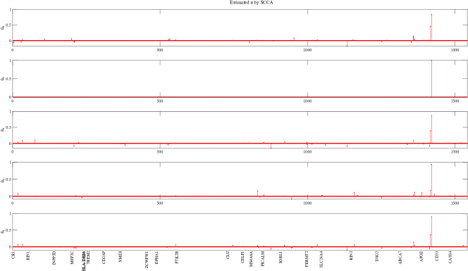
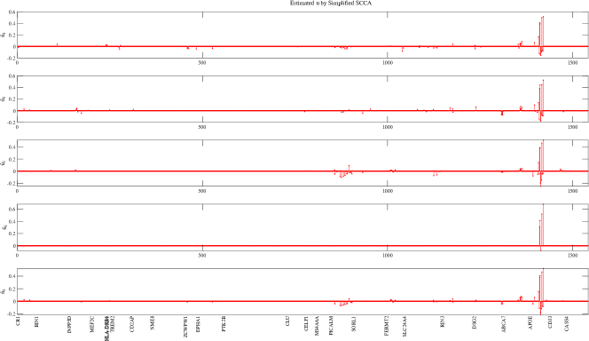
Figure S5: Canonical genetic weights estimated by SCCA (top figure) and simplified SCCA (bottom figure). In each figure, the results on each of the four training folds (rows 1-4) and on the entire data (bottom row) are shown.

The two SCCA models were applied to the ADNI data to identify bi-multivariate imaging genetics associations. We employed the nested five-fold cross-validation (which is an extension of the procedure described in Section V-A3) to choose the regularization parameters and report the performance. The genetic and imaging feature selection results are reported in Figures S5-S7 and Tables LABEL:tab:snps_selected-LABEL:tab:QTs_selected in Supplementary Materials Section E, while the canonical correlation/covariance performance is reported in Table II.

For genetic feature selection (Figure S5 and Table LABEL:tab:snps_selected), both SCCA models select top AD risk genes such as APOE, PICALM and ABCA7. However, in each gene, the simplified SCCA selects a cluster of SNPs while the standard SCCA only selects one or very few SNPs which dominate. Together with the correlation among the SNPs within each gene (Fig. S4 middle), it verifies that the simplified SCCA has the grouping effects in feature selection while the standard SCCA does not.

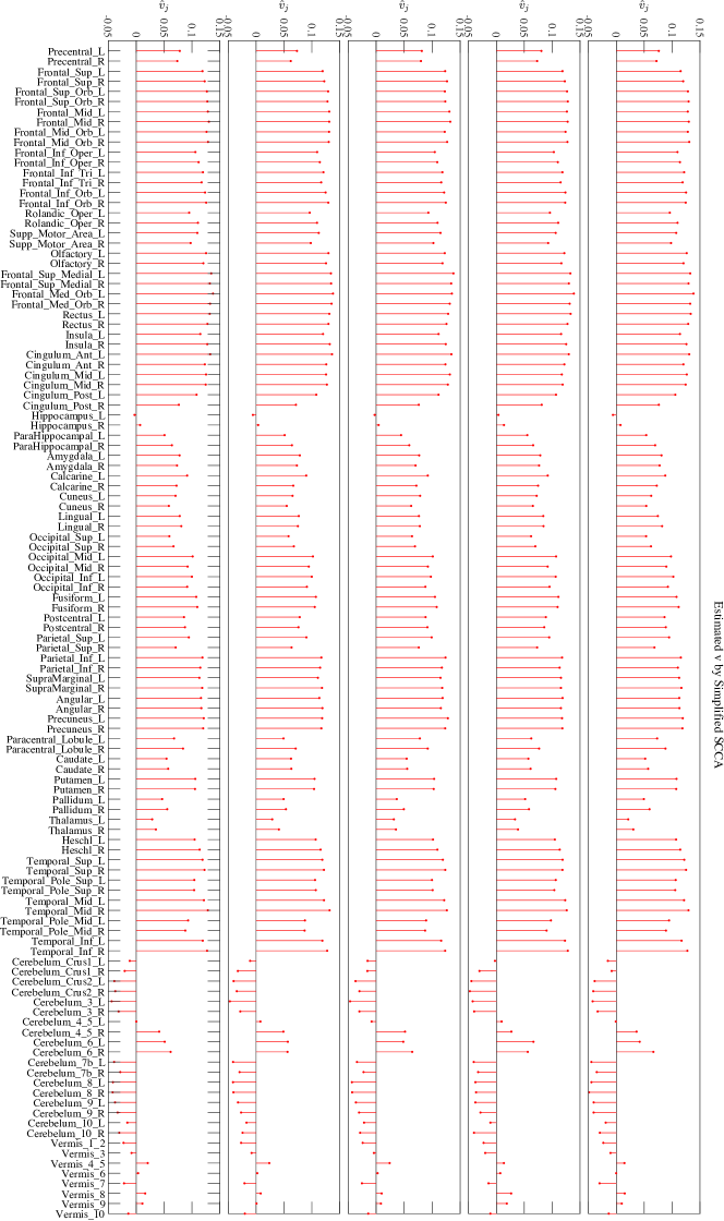
Figure S7: Canonical imaging weights estimated by SCCA (top figure) and simplified SCCA (bottom figure). In each figure, the results on each of the four training folds (rows 1-4) and on the entire data (bottom row) are shown.

For imaging feature selection (Figure S7 and Table LABEL:tab:QTs_selected), although high correlation is prevalent among the 116 imaging features (Fig. S4 right), the standard SCCA only selects about 20 features while the simplified SCCA selects more than 60 features, which confirms that the simplified SCCA is prone to selecting correlated feature together.

VI Conclusion

The sparse canonical correlation analysis (SCCA) is a bi-multivariate model that maximizes the multivariate correlation between two sets of variables. Since SCCA is computationally expensive, a simplified SCCA model which maximizes the multivariate covariance, has been widely used as its surrogate. The fundamental properties of the solutions of these two models remain unknown. Through theoretical analysis, we show that these two models behave differently regarding the grouping effects in variable selection. The simplified SCCA jointly selects or deselects a group of correlated variables together, while the standard SCCA randomly selects one or few representatives from a group of correlated variables. Empirical results on both synthetic and real data confirm our theoretical finding. This result can guide users to choose the right SCCA model in practice.

Study on the grouping effects of two sparse CCA models in variable selection
Supplementary materials

Appendix A Linearized ADMM to solve subproblem (30)

We present how to solve problem (30) using the linearized alternating direction method of multipliers (ADMM) [29, 15]. The problem (31) can be solved in a similar manner.

First, we write problem (30) in the form:

$$\underset{\mathbf{u}}{\text{minimize}}\;-\mathbf{u}^{\rm T}\mathbf{X}^{\rm T}\mathbf{Y}\mathbf{v}+\mathbf{1}\left(\left\|\mathbf{X}\mathbf{u}\right\|^{2}\leq 1\right)+\mathbf{1}\left(\left\|\mathbf{u}\right\|_{1}\leq c_{1}\right),$$ (36)

where $\mathbf{1}\left(\cdot\right)$ is the indicator function defined as

$$\mathbf{1}\left(\mathbf{x}\in\mathbb{A}\right)=\begin{cases}0,&\mathbf{x}\in\mathbb{A}\\ \infty,&\mathbf{x}\notin\mathbb{A}\end{cases}$$

To apply the ADMM, the problem (36) is reformulated as

$$\underset{\mathbf{u}}{\text{minimize}} -\mathbf{u}^{\rm T}\mathbf{X}^{\rm T}\mathbf{Y}\mathbf{v}+\mathbf{1}\left(\left\|\mathbf{z}\right\|^{2}\leq 1\right)+\mathbf{1}\left(\left\|\mathbf{u}\right\|_{1}\leq c_{1}\right)$$ (37)

subject to $$\mathbf{X}\mathbf{u}=\mathbf{z}$$

The augmented Lagrangian of problem (37) is

$$\mathcal{L}_{\rho}\left(\mathbf{u},\mathbf{z},\mathbf{\lambda}\right)=-\mathbf{u}^{\rm T}\mathbf{X}^{\rm T}\mathbf{Y}\mathbf{v}+\mathbf{1}\left(\left\|\mathbf{z}\right\|^{2}\leq 1\right)+\mathbf{1}\left(\left\|\mathbf{u}\right\|_{1}\leq c_{1}\right)+\left\langle\mathbf{\lambda},\mathbf{X}\mathbf{u}-\mathbf{z}\right\rangle+\frac{\rho}{2}\left\|\mathbf{X}\mathbf{u}-\mathbf{z}\right\|^{2}.$$ (38)

ADMM consists of the iterations:

$$\mathbf{u}_{\ell+1} =\operatorname*{argmin}_{\mathbf{u}}\mathcal{L}_{\rho}\left(\mathbf{u},\mathbf{z}_{\ell},\mathbf{\lambda}_{\ell}\right)$$ (39)

$$\mathbf{z}_{\ell+1} =\operatorname*{argmin}_{\mathbf{z}}\mathcal{L}_{\rho}\left(\mathbf{u}_{\ell+1},\mathbf{z},\mathbf{\lambda}_{\ell}\right)$$ (40)

$$\mathbf{\lambda}_{\ell+1} =\mathbf{\lambda}_{\ell}+\rho\left(\mathbf{X}\mathbf{u}_{\ell+1}-\mathbf{z}_{\ell+1}\right)$$ (41)

That is

$$\mathbf{u}_{\ell+1} =\operatorname*{argmin}_{\mathbf{u}}-\mathbf{u}^{\rm T}\mathbf{X}^{\rm T}\mathbf{Y}\mathbf{v}+\mathbf{1}\left(\left\|\mathbf{u}\right\|_{1}\leq c_{1}\right)+\left\langle\mathbf{\lambda}_{\ell},\mathbf{X}\mathbf{u}-\mathbf{z}_{\ell}\right\rangle+\frac{\rho}{2}\left\|\mathbf{X}\mathbf{u}-\mathbf{z}_{\ell}\right\|^{2}$$ (42)

$$\mathbf{z}_{\ell+1} =\operatorname*{argmin}_{\mathbf{z}}\mathbf{1}\left(\left\|\mathbf{z}\right\|^{2}\leq 1\right)+\left\langle\mathbf{\lambda}_{\ell},\mathbf{X}\mathbf{u}_{\ell+1}-\mathbf{z}\right\rangle+\frac{\rho}{2}\left\|\mathbf{X}\mathbf{u}_{\ell+1}-\mathbf{z}\right\|^{2}$$ (43)

$$\mathbf{\lambda}_{\ell+1} =\mathbf{\lambda}_{\ell}+\rho\left(\mathbf{X}\mathbf{u}_{\ell+1}-\mathbf{z}_{\ell+1}\right)$$ (44)

The problem (42) is not easy to solve due to the term $\frac{1}{2}\left\|\mathbf{X}\mathbf{u}-\mathbf{z}_{\ell}\right\|^{2}\triangleq f(\mathbf{u})$. To handle this, we construct a quadratic approximation of $f(\mathbf{u})$ near the estimate $\mathbf{u}_{\ell}$ of $\mathbf{u}$ in the previous iteration $\ell$:

$$F(\mathbf{u}) \triangleq f(\mathbf{u}_{\ell})+\left\langle\nabla f(\mathbf{u}_{\ell}),\mathbf{u}-\mathbf{u}_{\ell}\right\rangle+\frac{L_{X}}{2}\left\|\mathbf{u}-\mathbf{u}_{\ell}\right\|^{2}$$

$$=\frac{1}{2}\left\|\mathbf{X}\mathbf{u}_{\ell}-\mathbf{z}_{\ell}\right\|^{2}+\left\langle\mathbf{X}^{\rm T}\left(\mathbf{X}\mathbf{u}_{\ell}-\mathbf{z}_{\ell}\right),\mathbf{u}-\mathbf{u}_{\ell}\right\rangle+\frac{L_{X}}{2}\left\|\mathbf{u}-\mathbf{u}_{\ell}\right\|^{2}$$ (45)

where $L_{X}=\lambda_{\rm max}\left(\mathbf{X}^{\rm T}\mathbf{X}\right)$, where $\lambda_{\rm max}\left(\cdot\right)$ is the largest eigenvalue of its argument/input. Note that we have $F(\mathbf{u})\geq f(\mathbf{u})$ for any $\mathbf{u}\in{}^{p\times 1}$ and $F(\mathbf{u}_{\ell})=f(\mathbf{u}_{\ell})$.

In the linearized ADMM, it solves the approximate version of problem (42) with the term $f(\mathbf{u})=\frac{1}{2}\left\|\mathbf{X}\mathbf{u}-\mathbf{z}_{\ell}\right\|^{2}$ replaced by $F(\mathbf{u})$:

$$\mathbf{u}_{\ell+1} =\operatorname*{argmin}_{\mathbf{u}}-\mathbf{u}^{\rm T}\mathbf{X}^{\rm T}\mathbf{Y}\mathbf{v}+\mathbf{1}\left(\left\|\mathbf{u}\right\|_{1}\leq c_{1}\right)+\left\langle\mathbf{\lambda}_{\ell},\mathbf{X}\mathbf{u}-\mathbf{z}_{\ell}\right\rangle+\rho F(\mathbf{u})$$

$$=\operatorname*{argmin}_{\mathbf{u}}\frac{\rho L_{X}}{2}\left\|\mathbf{u}-\mathbf{u}_{\ell}+\frac{1}{L_{X}}\mathbf{X}^{\rm T}\left(\mathbf{X}\mathbf{u}_{\ell}-\mathbf{z}_{\ell}+\frac{1}{\rho}\mathbf{\lambda}_{\ell}-\frac{1}{\rho}\mathbf{Y}\mathbf{v}\right)\right\|+\mathbf{1}\left(\left\|\mathbf{u}\right\|_{1}\leq c_{1}\right)$$

$$={\rm prox}_{L1}\left(\mathbf{u}_{\ell}-\frac{1}{L_{X}}\mathbf{X}^{\rm T}\left(\mathbf{X}\mathbf{u}_{\ell}-\mathbf{z}_{\ell}+\frac{1}{\rho}\mathbf{\lambda}_{\ell}-\frac{1}{\rho}\mathbf{Y}\mathbf{v}\right);c_{1}\right)$$ (46)

where the proximal operator ${\rm prox}_{L1}\left(\cdot;\cdot\right)$ is defined as

$${\rm prox}_{L1}\left(\mathbf{a};c\right)=\operatorname*{argmin}_{\mathbf{x}}\;\frac{1}{2}\left\|\mathbf{x}-\mathbf{a}\right\|^{2}+\mathbf{1}\left(\left\|\mathbf{x}\right\|_{1}\leq c\right)=\begin{cases}\mathbf{a},&\left\|\mathbf{a}\right\|_{1}\leq c\\ \mathop{{\rm S}}\left(\mathbf{a},\Delta\right),&\left\|\mathbf{a}\right\|_{1}>c\end{cases}$$ (47)

where $\Delta$ is a positive constant that satisfies $\left\|\mathop{{\rm S}}\left(\mathbf{a},\Delta\right)\right\|_{1}=c$.

The update formula of problem (43) is

$$\mathbf{z}_{\ell+1}=\begin{cases}\mathbf{X}\mathbf{u}_{\ell+1}+\mathbf{\lambda}_{\ell}/\rho,&\left\|\mathbf{X}\mathbf{u}_{\ell+1}+\mathbf{\lambda}_{\ell}/\rho\right\|\leq 1\\ \frac{\mathbf{X}\mathbf{u}_{\ell+1}+\mathbf{\lambda}_{\ell}/\rho}{\left\|\mathbf{X}\mathbf{u}_{\ell+1}+\mathbf{\lambda}_{\ell}/\rho\right\|},&\left\|\mathbf{X}\mathbf{u}_{\ell+1}+\mathbf{\lambda}_{\ell}/\rho\right\|>1\end{cases}$$ (48)

Taken together, the updates at each ADMM iteration are

$$\mathbf{u}_{\ell+1} ={\rm prox}_{L1}\left(\mathbf{u}_{\ell}-\frac{1}{L_{X}}\mathbf{X}^{\rm T}\left(\mathbf{X}\mathbf{u}_{\ell}-\mathbf{z}_{\ell}+\mathbf{\xi}_{\ell}-\frac{1}{\rho}\mathbf{Y}\mathbf{v}\right);c_{1}\right)$$ (49)

$$\mathbf{z}_{\ell+1} =\begin{cases}\mathbf{X}\mathbf{u}_{\ell+1}+\mathbf{\xi}_{\ell},&\left\|\mathbf{X}\mathbf{u}_{\ell+1}+\mathbf{\xi}_{\ell}\right\|\leq 1\\ \frac{\mathbf{X}\mathbf{u}_{\ell+1}+\mathbf{\xi}_{\ell}}{\left\|\mathbf{X}\mathbf{u}_{\ell+1}+\mathbf{\xi}_{\ell}\right\|},&\left\|\mathbf{X}\mathbf{u}_{\ell+1}+\mathbf{\xi}_{\ell}\right\|>1\end{cases}$$ (50)

$$\mathbf{\xi}_{\ell+1} =\mathbf{\xi}_{\ell}+\mathbf{X}\mathbf{u}_{\ell+1}-\mathbf{z}_{\ell+1}$$ (51)

where $\mathbf{\xi}_{\ell}=\mathbf{\lambda}_{\ell}/\rho$.

The Linearized ADMM algorithm for fitting the SCCA model is summarized in Algorithm 3.

Algorithm 3 Sparse CCA fitting algorithm: Linearized ADMM

0:  $\mathbf{X}\in{}^{n\times p}$, $\mathbf{Y}\in{}^{n\times q}$, with column-wise zero empirical mean (the sample mean of each column has been shifted to zero); Regularization parameters $c_{1}$ and $c_{2}$.

1:  Calculate Lipschitz constants: $L_{X}=\lambda_{\rm max}\left(\mathbf{X}^{\rm T}\mathbf{X}\right)$, $L_{Y}=\lambda_{\rm max}\left(\mathbf{Y}^{\rm T}\mathbf{Y}\right)$;

2:  Initialization: $\mathbf{u}^{(0)}\in{}^{p\times 1},\mathbf{v}^{(0)}\in{}^{q\times 1}$;

3:  Set the penalty parameter to $\rho_{1}=\rho_{2}=1$ [29];

4:  $k=0$;

5:  repeat

6:     Update $\mathbf{u}$:

7:     $\mathbf{a}=\mathbf{Y}\mathbf{v}^{(k)}$

8:     Input: $\mathbf{u}_{0}=\mathbf{u}^{(k)}\in{}^{p\times 1}$, $\mathbf{z}_{0}=\mathbf{\xi}_{0}=\mathbf{0}\in{}^{n\times 1}$;

9:     for $\ell=0,1,2,\dots$ do

10:        

$$\mathbf{u}_{\ell+1} ={\rm prox}_{L1}\left(\mathbf{u}_{\ell}-\frac{1}{L_{X}}\mathbf{X}^{\rm T}\left(\mathbf{X}\mathbf{u}_{\ell}-\mathbf{z}_{\ell}+\mathbf{\xi}_{\ell}-\frac{1}{\rho_{1}}\mathbf{a}\right);c_{1}\right)$$

$$\mathbf{z}_{\ell+1} =\begin{cases}\mathbf{X}\mathbf{u}_{\ell+1}+\mathbf{\xi}_{\ell},&\left\|\mathbf{X}\mathbf{u}_{\ell+1}+\mathbf{\xi}_{\ell}\right\|\leq 1\\ \frac{\mathbf{X}\mathbf{u}_{\ell+1}+\mathbf{\xi}_{\ell}}{\left\|\mathbf{X}\mathbf{u}_{\ell+1}+\mathbf{\xi}_{\ell}\right\|},&\left\|\mathbf{X}\mathbf{u}_{\ell+1}+\mathbf{\xi}_{\ell}\right\|>1\end{cases}$$

$$\mathbf{\xi}_{\ell+1} =\mathbf{\xi}_{\ell}+\mathbf{X}\mathbf{u}_{\ell+1}-\mathbf{z}_{\ell+1}$$

11:     end for

12:     Output: $\mathbf{u}^{(k+1)}=\mathbf{u}_{\ell+1}$.  

13:     Update $\mathbf{v}$:

14:     $\mathbf{b}=\mathbf{X}\mathbf{u}^{(k+1)}$

15:     Initialization: $\mathbf{v}_{0}=\mathbf{v}^{(k)}\in{}^{q\times 1}$, $\mathbf{\zeta}_{0}=\mathbf{\psi}_{0}=\mathbf{0}\in{}^{n\times 1}$;

16:     for $\ell=0,1,2,\dots$ do

17:        

$$\mathbf{v}_{\ell+1} ={\rm prox}_{L1}\left(\mathbf{v}_{\ell}-\frac{1}{L_{Y}}\mathbf{Y}^{\rm T}\left(\mathbf{Y}\mathbf{v}_{\ell}-\mathbf{\zeta}_{\ell}+\mathbf{\psi}_{\ell}-\frac{1}{\rho_{2}}\mathbf{b}\right);c_{2}\right)$$

$$\mathbf{\zeta}_{\ell+1} =\begin{cases}\mathbf{Y}\mathbf{v}_{\ell+1}+\mathbf{\psi}_{\ell},&\left\|\mathbf{Y}\mathbf{v}_{\ell+1}+\mathbf{\psi}_{\ell}\right\|\leq 1\\ \frac{\mathbf{Y}\mathbf{v}_{\ell+1}+\mathbf{\psi}_{\ell}}{\left\|\mathbf{Y}\mathbf{v}_{\ell+1}+\mathbf{\psi}_{\ell}\right\|},&\left\|\mathbf{Y}\mathbf{v}_{\ell+1}+\mathbf{\psi}_{\ell}\right\|>1\end{cases}$$

$$\mathbf{\psi}_{\ell+1} =\mathbf{\psi}_{\ell}+\mathbf{Y}\mathbf{v}_{\ell+1}-\mathbf{\zeta}_{\ell+1}$$

18:     end for

19:     Output: $\mathbf{v}^{(k+1)}=\mathbf{v}_{\ell+1}$.

20:     $k\leftarrow k+1$.

21:  until convergence.

Appendix B Proof of Lemma IV.1 and how it extends Lemma 2.2 of [17]

B-A Proof of Lemma IV.1

Proof.

Since the problem (32) is a convex optimization problem with differentiable objective and constraint functions (Note that the L1 inequality constraint can be written as $2^{p}$ linear inequality constraints), and is strictly feasible (Slater’s condition holds), the KKT conditions provide necessary and sufficient conditions for optimality [27].

The Lagrangian function is

$$\mathcal{L}\left(\mathbf{u},\alpha,\Delta\right)=-\mathbf{a}^{\rm T}\mathbf{u}+\frac{\alpha}{2}\left(\left\|\mathbf{u}\right\|^{2}-1\right)+\Delta\left(\left\|\mathbf{u}\right\|_{1}-c\right)$$

where $\alpha$ and $\Delta$ are the Lagrange multipliers (dual variables) for the L2 and L1 constraints, respectively.

Setting the differential of $\mathcal{L}\left(\mathbf{u},\alpha,\Delta\right)$ with respect to $\mathbf{u}$ equal to zero yields

$$\alpha\mathbf{u}+\Delta\mathbf{s}=\mathbf{a}$$ (52)

where $\mathbf{s}$ is the subgradient of $\left\|\mathbf{u}\right\|_{1}$ with respect to $\mathbf{u}$, with $s_{i}=\mathop{{\rm sign}}\left(u_{i}\right)$ if $u_{i}\neq 0$ and $s_{i}\in[-1,1]$ otherwise.

The KKT conditions for optimality consist of (52) and

$$\alpha\geq 0,\quad\left\|\mathbf{u}\right\|^{2}\leq 1,\quad\alpha\left(\left\|\mathbf{u}\right\|^{2}-1\right)=0$$ (53)

$$\Delta\geq 0,\quad\left\|\mathbf{u}\right\|_{1}\leq c,\quad\Delta\left(\left\|\mathbf{u}\right\|_{1}-c\right)=0$$ (54)

• Case 1: $\alpha=0$, $\Delta>0$.

  The KKT conditions (52)-(54) are simplified as

  $$\Delta\mathbf{s} =\mathbf{a},\;\Delta>0$$ (55)

  $$\left\|\mathbf{u}\right\|^{2} \leq 1$$ (56)

  $$\left\|\mathbf{u}\right\|_{1} =c$$ (57)

  From (55), it follows that $\Delta=\max_{1\leq i\leq p}\left|a_{i}\right|$ and $u_{i}=0$ for any $i\notin{\mathcal{S}}$, where ${\mathcal{S}}=\left\{i\mid\;\left|a_{i}\right|=\Delta\right\}$.

  Therefore, an optimal solution can be written in the following form:

  $$[\mathbf{u}^{*}]_{i}=\begin{cases}w_{i}\mathop{{\rm sign}}\left(a_{i}\right),&i\in{\mathcal{S}}\\ 0,&i\notin{\mathcal{S}}\end{cases}$$ (58)

  with $w_{i}\geq 0$ satisfying

  $$\sum_{i\in{\mathcal{S}}}w_{i}^{2}\leq 1,\quad\sum_{i\in{\mathcal{S}}}w_{i}=c$$

  When $c\leq\sqrt{\left|{\mathcal{S}}\right|}$, the set of solutions defined above is non-empty, and among them the solution with minimum Euclidean norm is shown in (33).

• Case 2: $\alpha>0$

  • Case 2.1: $\Delta=0$

  The KKT conditions (52)-(54) are simplified as

  $$\alpha\mathbf{u} =\mathbf{a},\;\alpha>0$$ (59)

  $$\left\|\mathbf{u}\right\|^{2} =1$$ (60)

  $$\left\|\mathbf{u}\right\|_{1} \leq c$$ (61)

  From (59)-(60), it follows that $\mathbf{u}=\frac{\mathbf{a}}{\left\|\mathbf{a}\right\|}$.

  When $c\geq\frac{\left\|\mathbf{a}\right\|_{1}}{\left\|\mathbf{a}\right\|}$, the above $\mathbf{u}$ also satisfies (61) and is therefore the optimal solution.

• Case 2.2: $\Delta>0$ The conditions (53)-(54) become

  $$\alpha>0,\quad\left\|\mathbf{u}\right\|^{2}=1$$ (62)

  $$\Delta>0,\quad\left\|\mathbf{u}\right\|_{1}=c$$ (63)

  Combining conditions (52) and (62)-(63), we obtain the optimal solution shown in Eq. (34). This corresponds to the range $\sqrt{\left|{\mathcal{S}}\right|}\leq c<\frac{\left\|\mathbf{a}\right\|_{1}}{\left\|\mathbf{a}\right\|}$.

∎

B-B How does Lemma IV.1 extend Lemma 2.2 of [17]?

Fig. S1 illustrates two particular scenarios of Case 1 in Lemma IV.1 for $p=2$ where Lemma 2.2 in [17] fails.

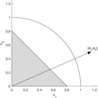
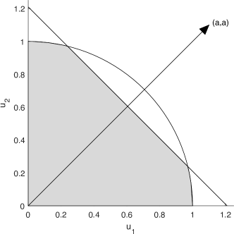
Figure S1: Two particular scenarios of Case 1 in Lemma IV.1 where Lemma 2.2 in [17] does not consider in the optimization problem. The dimension is $p=2$. The shaded area shows the domain [feasible/constraint set/region] (defined by the L2 and L1 constraints) of the objective function of problem (32). (a) $c=0.8<1$; (b) $c=1.25<\sqrt{2}$ and $a_{1}=a_{2}=a$. In both cases, the optimal solution in (a) (the point $\mathbf{u}*=[0.8;0]$) and the optimal solution in (b) (any point on the chord of the circle) do not have a form that is shown in Lemma 2.2 in [17].

Essentially, the expression presented in Lemma 2.2 of [17] is the solution to

$$\underset{\mathbf{u}}{\text{maximize}}\;\mathbf{a}^{\rm T}\mathbf{u}\quad\text{subject to }\left\|\mathbf{u}\right\|^{2}=1,\left\|\mathbf{u}\right\|_{1}\leq c$$ (64)

while in the problem (32) that Lemma IV.1 is solving, the L2 equality constraint is replaced by the L2 inequality constraint, resulting in a convex problem.

Note that in order for problem (64) to have an optimal solution of the form presented in Lemma 2.2 of [17], $c$ must be larger than or equal to $\sqrt{\left|{\mathcal{S}}\right|}$, where ${\mathcal{S}}$ is a set defined as ${\mathcal{S}}=\left\{i:i\in\operatorname*{argmax}_{j}\left|a_{j}\right|\right\}$ (see the proof of Lemma IV.1). Otherwise,

• when $0\leq c<1$, problem (64) is infeasible (there are no feasible points that satisfy the constraints).

• when $1<c<\sqrt{\left|{\mathcal{S}}\right|}$, the optimal solution to problem (64) is

  $$[\mathbf{u}^{*}]_{i}=\begin{cases}w_{i}\mathop{{\rm sign}}\left(a_{i}\right),&i\in{\mathcal{S}}\\ 0,&i\notin{\mathcal{S}}\end{cases}$$ (65a)

  where $$w_{i}\geq 0 i\in{\mathcal{S}}$$, , satisfy

  $$\sum_{i\in{\mathcal{S}}}w_{i}^{2}=1,\quad\sum_{i\in{\mathcal{S}}}w_{i}=c$$ (65b)

Note that solution (65) cannot be written in the form shown in Lemma 2.2 in [17].

By contrast, problem (32) has an optimal solution for every $c\geq 0$.

Appendix C How to obtain multiple canonical components of SCCA model sequentially?

In this section, we will show how to apply the single-canonical-component SCCA algorithms to sequentially compute multiple canonical components of standard and simplified SCCA models. Note that except that Algorithm 8 was described in [17], all algorithms (Algorithms 4-5 for standard the SCCA model and Algorithm 9 for the simplified SCCA model) and their theoretical justifications in Sections C-A1 and C-B1 are new, to the best our knowledge.

C-A Sequential calculation of multiple canonical components of standard SCCA

The SCCA model for computing $R$ canonical components is

$$\underset{\mathbf{U},\mathbf{V}}{\text{maximize}} \mathop{{\rm trace}}\left(\mathbf{U}^{\rm T}\mathbf{\hat{\Sigma}}_{\mathbf{xy}}\mathbf{V}\right)$$ (66)

subject to $$\mathbf{U}^{\rm T}\mathbf{\hat{\Sigma}}_{\mathbf{xx}}\mathbf{U}=\mathbf{I}_{R},\left\|\mathbf{u}_{r}\right\|_{1}\leq c_{1r},r=1,2,\dots,R$$

$$\mathbf{V}^{\rm T}\mathbf{\hat{\Sigma}}_{\mathbf{yy}}\mathbf{V}=\mathbf{I}_{R},\left\|\mathbf{v}_{r}\right\|_{1}\leq c_{2r},r=1,2,\dots,R$$

where

$$\mathbf{\hat{\Sigma}}_{\mathbf{xy}} =\frac{1}{n-1}\mathbf{X}^{\rm T}\mathbf{Y}$$ (67)

$$\mathbf{\hat{\Sigma}}_{\mathbf{xx}} =\frac{1}{n-1}\mathbf{X}^{\rm T}\mathbf{X}$$ (68)

$$\mathbf{\hat{\Sigma}}_{\mathbf{yy}} =\frac{1}{n-1}\mathbf{Y}^{\rm T}\mathbf{Y}$$ (69)

are the sample cross-covariance between random vectors $\mathbf{x}$ and $\mathbf{y}$, sample auto-covariance matrix within random vector $\mathbf{x}$ and sample auto-covariance matrix within random vector $\mathbf{y}$, respectively. Here we assume that the columns of $\mathbf{X}$ and $\mathbf{Y}$ have been centered to zero mean.

For clarity, we first present two algorithms (Algorithms 4 and 5) to sequentially compute multiple canonical components of SCCA: one is based on deflation of the cross-covariance matrix, and the other one is based on deflation of the data matrices. Then we provide theoretical explanations of both algorithms in the subsequent sections.

Algorithm 4 Sequential computation of $R$ canonical components of SCCA via deflation of the cross-covariance matrix.

1:  Let $\mathbf{\hat{\Sigma}}_{\mathbf{xy}}^{0}=\frac{1}{n-1}\mathbf{X}^{\rm T}\mathbf{Y}\in{}^{p\times q}$, $\mathbf{\hat{\Sigma}}_{\mathbf{xx}}=\frac{1}{n-1}\mathbf{X}^{\rm T}\mathbf{X}\in{}^{p\times p}$ and $\mathbf{\hat{\Sigma}}_{\mathbf{yy}}=\frac{1}{n-1}\mathbf{Y}^{\rm T}\mathbf{Y}\in{}^{q\times q}$.

2:  for $r=1,2,\dots,R$ do

3:     Find the $r$-th pair of canonical weight vectors $\mathbf{\hat{u}}_{r}$ and $\mathbf{\hat{v}}_{r}$ by applying the single-canonical-component SCCA algorithm to $\left(\mathbf{\hat{\Sigma}}_{\mathbf{xy}}^{r-1},\mathbf{\hat{\Sigma}}_{\mathbf{xx}},\mathbf{\hat{\Sigma}}_{\mathbf{yy}}\right)$:

$$\underset{\mathbf{u}_{r},\mathbf{v}_{r}}{\text{maximize}} \mathbf{u}_{r}^{\rm T}\mathbf{\hat{\Sigma}}_{\mathbf{xy}}^{r-1}\mathbf{v}_{r}$$

subject to $$\mathbf{u}_{r}^{\rm T}\mathbf{\hat{\Sigma}}_{\mathbf{xx}}\mathbf{u}_{r}\leq 1,\left\|\mathbf{u}_{r}\right\|_{1}\leq c_{1r}$$

$$\mathbf{v}_{r}^{\rm T}\mathbf{\hat{\Sigma}}_{\mathbf{yy}}\mathbf{v}_{r}\leq 1,\left\|\mathbf{v}_{r}\right\|_{1}\leq c_{2r}$$

4:     $\mathbf{\hat{\Sigma}}_{\mathbf{xy}}^{r}\leftarrow\mathbf{\hat{\Sigma}}_{\mathbf{xy}}^{r-1}-\mathbf{\hat{\Sigma}}_{\mathbf{xx}}\hat{d}_{r}\mathbf{\hat{u}}_{r}\mathbf{\hat{v}}_{r}^{\rm T}\mathbf{\hat{\Sigma}}_{\mathbf{yy}}$, where $\hat{d}_{r}=\frac{\mathbf{\hat{u}}_{r}^{\rm T}\mathbf{\hat{\Sigma}}_{\mathbf{xy}}^{r-1}\mathbf{\hat{v}}_{r}}{\mathbf{\hat{u}}_{r}^{\rm T}\mathbf{\hat{\Sigma}}_{\mathbf{xx}}\mathbf{\hat{u}}_{r}\cdot\mathbf{\hat{v}}_{r}^{\rm T}\mathbf{\hat{\Sigma}}_{\mathbf{yy}}\mathbf{\hat{v}}_{r}}$.

5:  end for

Algorithm 5 Sequential computation of $R$ canonical components of SCCA via deflation of the data matrices.

1:  Let $\mathbf{X}^{0}=\mathbf{X}\in{}^{n\times p}$, $\mathbf{Y}^{0}=\mathbf{Y}\in{}^{n\times q}$.

2:  for $r=1,2,\dots,R$ do

3:     Find the $r$-th pair of canonical weight vectors $\left(\mathbf{\hat{u}}_{r},\mathbf{\hat{v}}_{r}\right)$ by applying Algorithm 3 to solve

$$\underset{\mathbf{u},\mathbf{v}}{\text{maximize}} \frac{1}{n-1}\mathbf{u}_{r}^{\rm T}{\mathbf{X}^{r-1}}^{\rm T}\mathbf{Y}^{r-1}\mathbf{v}_{r}$$

subject to $$\frac{1}{n-1}\mathbf{u}_{r}^{\rm T}\mathbf{X}^{\rm T}\mathbf{X}\mathbf{u}_{r}\leq 1,\left\|\mathbf{u}_{r}\right\|_{1}\leq c_{1r}$$

$$\frac{1}{n-1}\mathbf{v}_{r}^{\rm T}\mathbf{Y}^{\rm T}\mathbf{Y}\mathbf{v}_{r}\leq 1,\left\|\mathbf{v}_{r}\right\|_{1}\leq c_{2r}$$

4:     Calculate the residual data:

$$\mathbf{X}^{r} \leftarrow\mathbf{X}^{r-1}-\mathbf{X}^{r-1}\frac{\mathbf{\hat{u}}_{r}\mathbf{\hat{u}}_{r}^{\rm T}\mathbf{X}^{\rm T}\mathbf{X}}{\mathbf{\hat{u}}_{r}^{\rm T}\mathbf{X}^{\rm T}\mathbf{X}\mathbf{\hat{u}}_{r}}$$ (70)

$$\mathbf{Y}^{r} \leftarrow\mathbf{Y}^{r-1}-\mathbf{Y}^{r-1}\frac{\mathbf{\hat{v}}_{r}\mathbf{\hat{v}}_{r}^{\rm T}\mathbf{Y}^{\rm T}\mathbf{Y}}{\mathbf{\hat{v}}_{r}^{\rm T}\mathbf{Y}^{\rm T}\mathbf{Y}\mathbf{\hat{v}}_{r}}$$ (71)

5:  end for

Remark C.1.

The deflated data in Eqs. (70)-(71) can also be interpreted as the residual matrix of linear least squares regression: $\underset{\mathbf{z}\in{}^{n}}{\text{minimize}}\;\left\|\mathbf{X}^{r-1}\left(\mathbf{X}^{\rm T}\mathbf{X}\right)^{-1/2}-\mathbf{z}\cdot\left[\left(\mathbf{X}^{\rm T}\mathbf{X}\right)^{1/2}\mathbf{\hat{u}}_{r}\right]^{\rm T}\right\|_{\rm F}^{2}$ and $\underset{\mathbf{\zeta}\in{}^{n}}{\text{minimize}}\;\left\|\mathbf{Y}^{r-1}\left(\mathbf{Y}^{\rm T}\mathbf{Y}\right)^{-1/2}-\mathbf{\zeta}\cdot\left[\left(\mathbf{Y}^{\rm T}\mathbf{Y}\right)^{1/2}\mathbf{\hat{v}}_{r}\right]^{\rm T}\right\|_{\rm F}^{2}$, respectively.

C-A1 Sequential calculation of multiple SCCA canonical components in the large-sample-size asymptotic regime

To compute $R$ canonical components sequentially/greedily, we consider the asymptotic regime of $n\to\infty$ in which case model (66) becomes

$$\underset{\mathbf{U},\mathbf{V}}{\text{maximize}} \mathop{{\rm trace}}\left(\mathbf{U}^{\rm T}\mathbf{\Sigma}_{\mathbf{xy}}\mathbf{V}\right)$$ (72)

subject to $$\mathbf{U}^{\rm T}\mathbf{\Sigma}_{\mathbf{xx}}\mathbf{U}=\mathbf{I}_{R}$$

$$\mathbf{V}^{\rm T}\mathbf{\Sigma}_{\mathbf{yy}}\mathbf{V}=\mathbf{I}_{R}$$

where $\mathbf{\Sigma}_{\mathbf{xy}}$, $\mathbf{\Sigma}_{\mathbf{xx}}$ and $\mathbf{\Sigma}_{\mathbf{yy}}$ are the population cross-covariance matrix between random vectors $\mathbf{x}$ and $\mathbf{y}$, population auto-covariance matrix within random vector $\mathbf{x}$ and population auto-covariance matrix within random vector $\mathbf{y}$, respectively. Note that in model (72) we have dropped the L1 regularizers: since we have infinite amount of data available for use, the L1 regularizations are no longer necessary.

The Lagrangian function of problem (72) is defined as

$$\mathcal{L}\left(\mathbf{U},\mathbf{V},\mathbf{\Psi},\mathbf{\Phi}\right)=-\mathbf{U}^{\rm T}\mathbf{\Sigma}_{\mathbf{xy}}\mathbf{V}+\left\langle\mathbf{\Psi},\mathbf{U}^{\rm T}\mathbf{\Sigma}_{\mathbf{xx}}\mathbf{U}-\mathbf{I}_{R}\right\rangle+\left\langle\mathbf{\Phi},\mathbf{V}^{\rm T}\mathbf{\Sigma}_{\mathbf{yy}}\mathbf{V}-\mathbf{I}_{R}\right\rangle$$

where $\mathbf{\Psi}\in{}^{R\times R}$ is a symmetric matrix of Lagrange multipliers for the $R(R+1)/2$ constraints on $\mathbf{U}$ in problem (72), and $\mathbf{\Phi}\in{}^{R\times R}$ is a symmetric matrix of Lagrange multipliers for the $R(R+1)/2$ constraints on $\mathbf{V}$.

Denote the optimal primal and dual solutions of problem (72) as $\left(\mathbf{\hat{U}},\mathbf{\hat{V}}\right)$ and $\left(\mathbf{\hat{\Psi}},\mathbf{\hat{\Phi}}\right)$, respectively. According to the KKT conditions, we have

$$2\mathbf{\Sigma}_{\mathbf{xx}}\mathbf{\hat{U}}\mathbf{\hat{\Psi}} =\mathbf{\Sigma}_{\mathbf{xy}}\mathbf{\hat{V}}$$ (73)

$$2\mathbf{\Sigma}_{\mathbf{yy}}\mathbf{\hat{V}}\mathbf{\hat{\Phi}} =\mathbf{\Sigma}_{\mathbf{xy}}^{\rm T}\mathbf{\hat{U}}$$ (74)

Combining Eqs. (73)-(74) with the quadratic constraints in problem (72) yields

$$2\mathbf{\hat{\Psi}} =\mathbf{\hat{U}}^{\rm T}\mathbf{\Sigma}_{\mathbf{xy}}\mathbf{\hat{V}}$$

$$2\mathbf{\hat{\Phi}} =\mathbf{\hat{V}}^{\rm T}\mathbf{\Sigma}_{\mathbf{xy}}^{\rm T}\mathbf{\hat{U}}$$

Note that problem (72) does not have a unique solution due to the rotational ambiguity: if $\left(\mathbf{\hat{U}},\mathbf{\hat{V}}\right)$ is an optimal solution of problem (72), then $\left(\mathbf{\hat{\hat{U}}},\mathbf{\hat{\hat{V}}}\right)=\left(\mathbf{\hat{U}}\mathbf{Q},\mathbf{\hat{V}}\mathbf{Q}\right)$ for any orthogonal matrix $\mathbf{Q}\in{}^{R\times R}$ is also an optimal solution. Since $\mathbf{\hat{\Psi}}$ and thus $\mathbf{\hat{U}}^{\rm T}\mathbf{\Sigma}_{\mathbf{xy}}\mathbf{\hat{V}}$ is a symmetric matrix, we can choose the optimal solution $\left(\mathbf{\hat{U}},\mathbf{\hat{V}}\right)$ for which $\mathbf{\hat{U}}^{\rm T}\mathbf{\Sigma}_{\mathbf{xy}}\mathbf{\hat{V}}$ is a diagonal matrix. As a result,

$$2\mathbf{\hat{\Psi}}=2\mathbf{\hat{\Phi}}\eqqcolon\mathbf{D}$$

is a diagonal matrix. Assuming both $\mathbf{\Sigma}_{\mathbf{xx}}$ and $\mathbf{\Sigma}_{\mathbf{yy}}$ are nonsingular, Eqs. (73)-(74) can be rewritten as

$$\mathbf{\Sigma}_{\mathbf{xx}}^{1/2}\mathbf{\hat{U}}\mathbf{D} =\mathbf{\Sigma}_{\mathbf{xx}}^{-1/2}\mathbf{\Sigma}_{\mathbf{xy}}\mathbf{\Sigma}_{\mathbf{yy}}^{-1/2}\cdot\mathbf{\Sigma}_{\mathbf{yy}}^{1/2}\mathbf{\hat{V}}$$ (75)

$$\mathbf{\Sigma}_{\mathbf{yy}}^{1/2}\mathbf{\hat{V}}\mathbf{D} =\mathbf{\Sigma}_{\mathbf{yy}}^{-1/2}\mathbf{\Sigma}_{\mathbf{xy}}^{\rm T}\mathbf{\Sigma}_{\mathbf{xx}}^{-1/2}\cdot\mathbf{\Sigma}_{\mathbf{xx}}^{1/2}\mathbf{\hat{U}}$$ (76)

Note that the objective of problem (72) is to maximize $\mathop{{\rm trace}}\left(\mathbf{D}\right)$ under the constraints that $\mathbf{\Sigma}_{\mathbf{xx}}^{1/2}\mathbf{U}$ and $\mathbf{\Sigma}_{\mathbf{yy}}^{1/2}\mathbf{V}$ both have orthonormal columns. It follows that $\mathbf{D}$ contains the $R$ largest singular values of $\mathbf{\Sigma}_{\mathbf{xx}}^{-1/2}\mathbf{\Sigma}_{\mathbf{xy}}\mathbf{\Sigma}_{\mathbf{yy}}^{-1/2}$, and $\mathbf{\hat{E}}=\mathbf{\Sigma}_{\mathbf{xx}}^{1/2}\mathbf{\hat{U}}$ and $\mathbf{\hat{F}}=\mathbf{\Sigma}_{\mathbf{yy}}^{1/2}\mathbf{\hat{V}}$ contain the corresponding $R$ left and right singular vectors, respectively. According to the Eckart-Young-Mirsky theorem [31], the columns of $\mathbf{\hat{U}}$ and $\mathbf{\hat{V}}$ can be obtained by successive rank-one SVDs of the residual covariance matrix. Specifically, let $\mathbf{S}^{0}=\mathbf{\Sigma}_{\mathbf{xx}}^{-1/2}\mathbf{\Sigma}_{\mathbf{xy}}\mathbf{\Sigma}_{\mathbf{yy}}^{-1/2}\in{}^{p\times q}$. For $r=1,2,\dots,R$, we have

$$\left(\hat{d}_{r},\mathbf{\hat{u}}_{r},\mathbf{\hat{v}}_{r}\right) =\operatorname*{argmin}_{\begin{subarray}{c}d_{r},\mathbf{u}_{r},\mathbf{v}_{r}\\ \left\|\mathbf{\Sigma}_{\mathbf{xx}}^{1/2}\mathbf{u}_{r}\right\|=1\\ \left\|\mathbf{\Sigma}_{\mathbf{yy}}^{1/2}\mathbf{v}_{r}\right\|=1\end{subarray}}\left\|\mathbf{S}^{r-1}-\mathbf{\Sigma}_{\mathbf{xx}}^{1/2}d_{r}\mathbf{u}_{r}\mathbf{v}_{r}^{\rm T}\mathbf{\Sigma}_{\mathbf{yy}}^{1/2}\right\|_{\rm F}^{2}$$ (77)

$$\mathbf{S}^{r} =\mathbf{S}^{r-1}-\mathbf{\Sigma}_{\mathbf{xx}}^{1/2}\hat{d}_{r}\mathbf{\hat{u}}_{r}\mathbf{\hat{v}}_{r}^{\rm T}\mathbf{\Sigma}_{\mathbf{yy}}^{1/2}$$ (78)

Suppose we have obtained the estimate of the $r$-th pair of canonical weight vectors $\left(\mathbf{\hat{u}}_{r},\mathbf{\hat{v}}_{r}\right)$. We then estimate $d_{r}$ as

$$\hat{d}_{r}=\operatorname*{argmin}_{d_{r}}\left\|\mathbf{S}^{r-1}-\mathbf{\Sigma}_{\mathbf{xx}}^{1/2}d_{r}\mathbf{\hat{u}}_{r}\mathbf{\hat{v}}_{r}^{\rm T}\mathbf{\Sigma}_{\mathbf{yy}}^{1/2}\right\|_{\rm F}^{2}=\frac{\mathbf{\hat{u}}_{r}^{\rm T}\mathbf{\Sigma}_{\mathbf{xx}}^{1/2}\mathbf{S}^{r-1}\mathbf{\Sigma}_{\mathbf{yy}}^{1/2}\mathbf{\hat{v}}_{r}}{\mathbf{\hat{u}}_{r}^{\rm T}\mathbf{\Sigma}_{\mathbf{xx}}\mathbf{\hat{u}}_{r}\cdot\mathbf{\hat{v}}_{r}^{\rm T}\mathbf{\Sigma}_{\mathbf{yy}}\mathbf{\hat{v}}_{r}}$$

Taken all together, to compute multiple canonical components sequentially in the large-sample-size asymptotic regime, the residual covariance matrix is updated as below:

$$\mathbf{S}^{0} =\mathbf{\Sigma}_{\mathbf{xx}}^{-1/2}\mathbf{\Sigma}_{\mathbf{xy}}\mathbf{\Sigma}_{\mathbf{yy}}^{-1/2}$$ (79)

$$\mathbf{S}^{r} =\mathbf{S}^{r-1}-\frac{\mathbf{\Sigma}_{\mathbf{xx}}^{1/2}\mathbf{\hat{u}}_{r}\mathbf{\hat{u}}_{r}^{\rm T}\mathbf{\Sigma}_{\mathbf{xx}}^{1/2}\mathbf{S}^{r-1}\mathbf{\Sigma}_{\mathbf{yy}}^{1/2}\mathbf{\hat{v}}_{r}\mathbf{\hat{v}}_{r}^{\rm T}\mathbf{\Sigma}_{\mathbf{yy}}^{1/2}}{\mathbf{\hat{u}}_{r}^{\rm T}\mathbf{\Sigma}_{\mathbf{xx}}\mathbf{\hat{u}}_{r}\cdot\mathbf{\hat{v}}_{r}^{\rm T}\mathbf{\Sigma}_{\mathbf{yy}}\mathbf{\hat{v}}_{r}},\;r=1,2,\dots,R$$ (80)

or equivalently

$$\mathbf{\Sigma}_{\mathbf{xy}}^{0} =\mathbf{\Sigma}_{\mathbf{xy}}$$ (81)

$$\mathbf{\Sigma}_{\mathbf{xy}}^{r} =\mathbf{\Sigma}_{\mathbf{xy}}^{r-1}-\frac{\mathbf{\Sigma}_{\mathbf{xx}}\mathbf{\hat{u}}_{r}\mathbf{\hat{u}}_{r}^{\rm T}\mathbf{\Sigma}_{\mathbf{xy}}^{r-1}\mathbf{\hat{v}}_{r}\mathbf{\hat{v}}_{r}^{\rm T}\mathbf{\Sigma}_{\mathbf{yy}}}{\mathbf{\hat{u}}_{r}^{\rm T}\mathbf{\Sigma}_{\mathbf{xx}}\mathbf{\hat{u}}_{r}\cdot\mathbf{\hat{v}}_{r}^{\rm T}\mathbf{\Sigma}_{\mathbf{yy}}\mathbf{\hat{v}}_{r}},\;r=1,2,\dots,R$$ (82)

which results in Algorithm 6.

Let $\mathbf{x}\in{}^{p\times 1}$ and $\mathbf{y}\in{}^{q\times 1}$ be random vectors generating the $\mathbf{X}\in{}^{n\times p}$ and $\mathbf{Y}\in{}^{n\times q}$, respectively. For notational simplicity, assume $\mathop{{\rm\mathbb{E}}}\left[\mathbf{x}\right]=\mathbf{0}$, $\mathop{{\rm\mathbb{E}}}\left[\mathbf{y}\right]=\mathbf{0}$. It can be shown that the residual covariance matrix update formulas (79)-(80) can be rewritten in terms of random vectors $\mathbf{x}$ and $\mathbf{y}$ as

$$\mathbf{x}^{0} =\mathbf{x},\;\mathbf{y}^{0}=\mathbf{y}$$ (83)

$$\mathbf{x}^{r} =\mathbf{\Sigma}_{\mathbf{xx}}^{1/2}\left(\mathbf{I}_{p}-\frac{\mathbf{\Sigma}_{\mathbf{xx}}^{1/2}\mathbf{\hat{u}}_{r}\mathbf{\hat{u}}_{r}^{\rm T}\mathbf{\Sigma}_{\mathbf{xx}}^{1/2}}{\mathbf{\hat{u}}_{r}^{\rm T}\mathbf{\Sigma}_{\mathbf{xx}}\mathbf{\hat{u}}_{r}}\right)\mathbf{\Sigma}_{\mathbf{xx}}^{-1/2}\mathbf{x}^{r-1}=\mathbf{x}^{r-1}-\frac{\mathbf{\Sigma}_{\mathbf{xx}}\mathbf{\hat{u}}_{r}\mathbf{\hat{u}}_{r}^{\rm T}}{\mathbf{\hat{u}}_{r}^{\rm T}\mathbf{\Sigma}_{\mathbf{xx}}\mathbf{\hat{u}}_{r}}\mathbf{x}^{r-1}$$ (84)

$$\mathbf{y}^{r} =\mathbf{\Sigma}_{\mathbf{yy}}^{1/2}\left(\mathbf{I}_{q}-\frac{\mathbf{\Sigma}_{\mathbf{yy}}^{1/2}\mathbf{\hat{v}}_{r}\mathbf{\hat{v}}_{r}^{\rm T}\mathbf{\Sigma}_{\mathbf{yy}}^{1/2}}{\mathbf{\hat{v}}_{r}^{\rm T}\mathbf{\Sigma}_{\mathbf{yy}}\mathbf{\hat{v}}_{r}}\right)\mathbf{\Sigma}_{\mathbf{yy}}^{-1/2}\mathbf{y}^{r-1}=\mathbf{y}^{r-1}-\frac{\mathbf{\Sigma}_{\mathbf{yy}}\mathbf{\hat{v}}_{r}\mathbf{\hat{v}}_{r}^{\rm T}}{\mathbf{\hat{v}}_{r}^{\rm T}\mathbf{\Sigma}_{\mathbf{yy}}\mathbf{\hat{v}}_{r}}\mathbf{y}^{r-1}$$ (85)

which results in Algorithm 7.

Algorithm 6 Sequential computation of $R$ canonical components of SCCA in asymptotic regime via deflation of the population cross-covariance matrix.

1:  $\mathbf{\Sigma}_{\mathbf{xy}}^{0}=\mathop{{\rm\mathbb{E}}}\left[\mathbf{x}\mathbf{y}^{\rm T}\right]$, $\mathbf{\Sigma}_{\mathbf{xx}}=\mathop{{\rm\mathbb{E}}}\left[\mathbf{x}\mathbf{x}^{\rm T}\right]$ and $\mathbf{\Sigma}_{\mathbf{yy}}=\mathop{{\rm\mathbb{E}}}\left[\mathbf{y}\mathbf{y}^{\rm T}\right]$.

2:  for $r=1,2,\dots,R$ do

3:     Find the estimate of the $r$-th pair of canonical weight vectors $\mathbf{\hat{u}}_{r}$ and $\mathbf{\hat{v}}_{r}$:

$$\underset{\mathbf{u}_{r},\mathbf{v}_{r}}{\text{maximize}} \mathbf{u}_{r}^{\rm T}\mathbf{\Sigma}_{\mathbf{xy}}^{r-1}\mathbf{v}_{r}$$

subject to $$\mathbf{u}_{r}^{\rm T}\mathbf{\Sigma}_{\mathbf{xx}}\mathbf{u}_{r}=1$$

$$\mathbf{v}_{r}^{\rm T}\mathbf{\Sigma}_{\mathbf{yy}}\mathbf{v}_{r}=1$$

4:     $\mathbf{\Sigma}_{\mathbf{xy}}^{r}\leftarrow\mathbf{\Sigma}_{\mathbf{xy}}^{r-1}-\mathbf{\Sigma}_{\mathbf{xx}}\hat{d}_{r}\mathbf{\hat{u}}_{r}\mathbf{\hat{v}}_{r}^{\rm T}\mathbf{\Sigma}_{\mathbf{yy}}$, where $\hat{d}_{r}=\frac{\mathbf{\hat{u}}_{r}^{\rm T}\mathbf{\Sigma}_{\mathbf{xy}}^{r-1}\mathbf{\hat{v}}_{r}}{\mathbf{\hat{u}}_{r}^{\rm T}\mathbf{\Sigma}_{\mathbf{xx}}\mathbf{\hat{u}}_{r}\cdot\mathbf{\hat{v}}_{r}^{\rm T}\mathbf{\Sigma}_{\mathbf{yy}}\mathbf{\hat{v}}_{r}}$.

5:  end for

Algorithm 7 Sequential computation of $R$ canonical components of SCCA in asymptotic regime via deflation of random vectors.

1:  Let $\mathbf{x}^{0}=\mathbf{x}\in{}^{p\times 1}$, $\mathbf{y}^{0}=\mathbf{y}\in{}^{q\times 1}$.

2:  for $r=1,2,\dots,R$ do

3:     Find the estimate of the $r$-th pair of canonical weight vectors $\mathbf{\hat{u}}_{r}$ and $\mathbf{\hat{v}}_{r}$:

$$\underset{\mathbf{u}_{r},\mathbf{v}_{r}}{\text{maximize}} \mathbf{u}_{r}^{\rm T}\mathop{{\rm\mathbb{E}}}\left[\mathbf{x}^{r-1}{\mathbf{y}^{r-1}}^{\rm T}\right]\mathbf{v}_{r}$$

subject to $$\mathbf{u}_{r}^{\rm T}\mathop{{\rm\mathbb{E}}}\left[\mathbf{x}\mathbf{x}^{\rm T}\right]\mathbf{u}_{r}=1$$

$$\mathbf{v}_{r}^{\rm T}\mathop{{\rm\mathbb{E}}}\left[\mathbf{y}\mathbf{y}^{\rm T}\right]\mathbf{v}_{r}=1$$

4:     Calculate the residual random vectors:

$$\mathbf{x}^{r} \leftarrow\mathbf{x}^{r-1}-\frac{\mathbf{\Sigma}_{\mathbf{xx}}\mathbf{\hat{u}}_{r}\mathbf{\hat{u}}_{r}^{\rm T}}{\mathbf{\hat{u}}_{r}^{\rm T}\mathbf{\Sigma}_{\mathbf{xx}}\mathbf{\hat{u}}_{r}}\mathbf{x}^{r-1}$$

$$\mathbf{y}^{r} \leftarrow\mathbf{y}^{r-1}-\frac{\mathbf{\Sigma}_{\mathbf{yy}}\mathbf{\hat{v}}_{r}\mathbf{\hat{v}}_{r}^{\rm T}}{\mathbf{\hat{v}}_{r}^{\rm T}\mathbf{\Sigma}_{\mathbf{yy}}\mathbf{\hat{v}}_{r}}\mathbf{y}^{r-1}$$

5:  end for

The Algorithms 4 and 5 are implementations of Algorithms 6 and 7 in finite-sample settings, respectively.

C-B Sequential calculation of multiple canonical components of simplified SCCA

The simplified SCCA model for computing $R$ canonical components is

$$\underset{\mathbf{U},\mathbf{V}}{\text{maximize}} \mathop{{\rm trace}}\left(\mathbf{U}^{\rm T}\mathbf{\hat{\Sigma}}_{\mathbf{xy}}\mathbf{V}\right)$$ (86)

subject to $$\mathbf{U}^{\rm T}\mathbf{U}=\mathbf{I}_{R},\left\|\mathbf{u}_{r}\right\|_{1}\leq c_{1r},r=1,2,\dots,R$$

$$\mathbf{V}^{\rm T}\mathbf{V}=\mathbf{I}_{R},\left\|\mathbf{v}_{r}\right\|_{1}\leq c_{2r},r=1,2,\dots,R$$

where $\mathbf{\hat{\Sigma}}_{\mathbf{xy}}$ is the sample cross-covariance matrix between random vectors $\mathbf{x}$ and $\mathbf{y}$.

For clarity, we first present two algorithms (Algorithms 8 and 9) to sequentially compute multiple canonical components of simplified SCCA: one is based on deflation of the cross-covariance matrix, and the other one is based on deflation of the data matrices. Then we provide theoretical explanations of both algorithms in the subsequent sections.

Algorithm 8 Sequential computation of $R$ canonical components of simplified SCCA via deflation of the cross-covariance matrix.

1:  Let $\mathbf{\hat{\Sigma}}_{\mathbf{xy}}^{0}=\frac{1}{n-1}\mathbf{X}^{\rm T}\mathbf{Y}\in{}^{p\times q}$.

2:  for $r=1,2,\dots,R$ do

3:     Find the $r$-th pair of canonical weight vectors $\mathbf{\hat{u}}_{r}$ and $\mathbf{\hat{v}}_{r}$ by applying Algorithm 2 to $\mathbf{\hat{\Sigma}}_{\mathbf{xy}}^{r-1}$:

$$\underset{\mathbf{u}_{r},\mathbf{v}_{r}}{\text{maximize}} \mathbf{u}_{r}^{\rm T}\mathbf{\hat{\Sigma}}_{\mathbf{xy}}^{r-1}\mathbf{v}_{r}$$

subject to $$\left\|\mathbf{u}_{r}\right\|^{2}\leq 1,\left\|\mathbf{u}_{r}\right\|_{1}\leq c_{1r}$$

$$\left\|\mathbf{v}_{r}\right\|^{2}\leq 1,\left\|\mathbf{v}_{r}\right\|_{1}\leq c_{2r}$$

4:     $\mathbf{\hat{\Sigma}}_{\mathbf{xy}}^{r}\leftarrow\mathbf{\hat{\Sigma}}_{\mathbf{xy}}^{r-1}-\hat{d}_{r}\mathbf{\hat{u}}_{r}\mathbf{\hat{v}}_{r}^{\rm T}$, where $\hat{d}_{r}=\frac{\mathbf{\hat{u}}_{r}^{\rm T}\mathbf{\hat{\Sigma}}_{\mathbf{xy}}^{r-1}\mathbf{\hat{v}}_{r}}{\left\|\mathbf{\hat{u}}_{r}\right\|^{2}\cdot\left\|\mathbf{\hat{v}}_{r}\right\|^{2}}$.

5:  end for

Algorithm 9 Sequential computation of $R$ canonical components of simplified SCCA via deflation of the data matrices.

1:  Let $\mathbf{X}^{0}=\mathbf{X}\in{}^{n\times p}$, $\mathbf{Y}^{0}=\mathbf{Y}\in{}^{n\times q}$.

2:  for $r=1,2,\dots,R$ do

3:     Find the $r$-th pair of canonical weight vectors $\left(\mathbf{\hat{u}}_{r},\mathbf{\hat{v}}_{r}\right)$ by applying Algorithm 2:

$$\underset{\mathbf{u},\mathbf{v}}{\text{maximize}} \frac{1}{n-1}\mathbf{u}_{r}^{\rm T}{\mathbf{X}^{r-1}}^{\rm T}\mathbf{Y}^{r-1}\mathbf{v}_{r}$$

subject to $$\left\|\mathbf{u}_{r}\right\|^{2}\leq 1,\left\|\mathbf{u}\right\|_{1}\leq c_{1r}$$

$$\left\|\mathbf{v}_{r}\right\|^{2}\leq 1,\left\|\mathbf{v}\right\|_{1}\leq c_{2r}$$

4:     Calculate the residual data:

$$\mathbf{X}^{r} \leftarrow\mathbf{X}^{r-1}\left(\mathbf{I}_{p}-\frac{\mathbf{\hat{u}}_{r}\mathbf{\hat{u}}_{r}^{\rm T}}{\left\|\mathbf{\hat{u}}_{r}\right\|^{2}}\right)$$ (87)

$$\mathbf{Y}^{r} \leftarrow\mathbf{Y}^{r-1}\left(\mathbf{I}_{q}-\frac{\mathbf{\hat{v}}_{r}\mathbf{\hat{v}}_{r}^{\rm T}}{\left\|\mathbf{\hat{v}}_{r}\right\|^{2}}\right)$$ (88)

5:  end for

Remark C.2.

The deflated data in Eqs. (87)-(88) can also be interpreted as the residual matrix of linear least squares regression: $\underset{\mathbf{z}\in{}^{n}}{\text{minimize}}\;\left\|\mathbf{X}^{r-1}-\mathbf{z}\cdot\mathbf{\hat{u}}_{r}^{\rm T}\right\|_{\rm F}^{2}$ and $\underset{\mathbf{\zeta}\in{}^{n}}{\text{minimize}}\;\left\|\mathbf{Y}^{r-1}-\mathbf{\zeta}\cdot\mathbf{\hat{v}}_{r}^{\rm T}\right\|_{\rm F}^{2}$, respectively.

C-B1 Sequential calculation of multiple SCCA canonical components in the large-sample-size asymptotic regime

To compute $R$ canonical components sequentially/greedily, we consider the asymptotic regime of $n\to\infty$ in which case model (86) becomes

$$\underset{\mathbf{U},\mathbf{V}}{\text{maximize}} \mathop{{\rm trace}}\left(\mathbf{U}^{\rm T}\mathbf{\Sigma}_{\mathbf{xy}}\mathbf{V}\right)$$ (89)

subject to $$\mathbf{U}^{\rm T}\mathbf{U}=\mathbf{I}_{R}$$

$$\mathbf{V}^{\rm T}\mathbf{V}=\mathbf{I}_{R}$$

where $\mathbf{\Sigma}_{\mathbf{xy}}$ is the population cross-covariance matrix between random vectors $\mathbf{x}$ and $\mathbf{y}$. Note that in model (89) we have dropped the L1 regularizers: since we have infinite amount of data available for use, the L1 regularizations are no longer necessary.

The Lagrangian function of problem (89) is defined as

$$\mathcal{L}\left(\mathbf{U},\mathbf{V},\mathbf{\Psi},\mathbf{\Phi}\right)=-\mathbf{U}^{\rm T}\mathbf{\Sigma}_{\mathbf{xy}}\mathbf{V}+\left\langle\mathbf{\Psi},\mathbf{U}^{\rm T}\mathbf{U}-\mathbf{I}_{R}\right\rangle+\left\langle\mathbf{\Phi},\mathbf{V}^{\rm T}\mathbf{V}-\mathbf{I}_{R}\right\rangle$$

where $\mathbf{\Psi}\in{}^{R\times R}$ is a symmetric matrix of Lagrange multipliers for the $R(R+1)/2$ constraints on $\mathbf{U}$ in problem (89), and $\mathbf{\Phi}\in{}^{R\times R}$ is a symmetric matrix of Lagrange multipliers for the $R(R+1)/2$ constraints on $\mathbf{V}$.

Denote the optimal primal and dual solutions of problem (89) as $\left(\mathbf{\hat{U}},\mathbf{\hat{V}}\right)$ and $\left(\mathbf{\hat{\Psi}},\mathbf{\hat{\Phi}}\right)$, respectively. According to the KKT conditions, we have

$$2\mathbf{\hat{U}}\mathbf{\hat{\Psi}} =\mathbf{\Sigma}_{\mathbf{xy}}\mathbf{\hat{V}}$$ (90)

$$2\mathbf{\hat{V}}\mathbf{\hat{\Phi}} =\mathbf{\Sigma}_{\mathbf{xy}}^{\rm T}\mathbf{\hat{U}}$$ (91)

Combining Eqs. (90)-(91) with the quadratic constraints in problem (89) yields

$$2\mathbf{\hat{\Psi}} =\mathbf{\hat{U}}^{\rm T}\mathbf{\Sigma}_{\mathbf{xy}}\mathbf{\hat{V}}$$

$$2\mathbf{\hat{\Phi}} =\mathbf{\hat{V}}^{\rm T}\mathbf{\Sigma}_{\mathbf{xy}}^{\rm T}\mathbf{\hat{U}}$$

Note that problem (89) does not have a unique solution due to the rotational ambiguity: if $\left(\mathbf{\hat{U}},\mathbf{\hat{V}}\right)$ is an optimal solution of problem (89), then $\left(\mathbf{\hat{\hat{U}}},\mathbf{\hat{\hat{V}}}\right)=\left(\mathbf{\hat{U}}\mathbf{Q},\mathbf{\hat{V}}\mathbf{Q}\right)$ for any orthogonal matrix $\mathbf{Q}\in{}^{R\times R}$ is also an optimal solution. Since $\mathbf{\hat{\Psi}}$ and thus $\mathbf{\hat{U}}^{\rm T}\mathbf{\Sigma}_{\mathbf{xy}}\mathbf{\hat{V}}$ is a symmetric matrix, we can choose the optimal solution $\left(\mathbf{\hat{U}},\mathbf{\hat{V}}\right)$ for which $\mathbf{\hat{U}}^{\rm T}\mathbf{\Sigma}_{\mathbf{xy}}\mathbf{\hat{V}}$ is a diagonal matrix. As a result,

$$2\mathbf{\hat{\Psi}}=2\mathbf{\hat{\Phi}}\eqqcolon\mathbf{D}$$

is a diagonal matrix. Assuming both $\mathbf{\Sigma}_{\mathbf{xx}}$ and $\mathbf{\Sigma}_{\mathbf{yy}}$ are nonsingular, Eqs. (90)-(91) can be rewritten as

$$\mathbf{\hat{U}}\mathbf{D} =\mathbf{\Sigma}_{\mathbf{xy}}\cdot\mathbf{\hat{V}}$$ (92)

$$\mathbf{\hat{V}}\mathbf{D} =\mathbf{\Sigma}_{\mathbf{xy}}^{\rm T}\cdot\mathbf{\hat{U}}$$ (93)

Note that the objective of problem (89) is to maximize $\mathop{{\rm trace}}\left(\mathbf{D}\right)$ under the constraints that $\mathbf{U}$ and $\mathbf{V}$ both have orthonormal columns. It follows that $\mathbf{D}$ contains the $R$ largest singular values of $\mathbf{\Sigma}_{\mathbf{xy}}$, and $\mathbf{\hat{U}}$ and $\mathbf{\hat{V}}$ contain the corresponding $R$ left and right singular vectors, respectively. According to the Eckart-Young-Mirsky theorem [31], the columns of $\mathbf{\hat{U}}$ and $\mathbf{\hat{V}}$ can be obtained by successive rank-one SVDs of the residual covariance matrix. Specifically, let $\mathbf{\Sigma}_{\mathbf{xy}}^{0}=\mathbf{\Sigma}_{\mathbf{xy}}\in{}^{p\times q}$. For $r=1,2,\dots,R$, we have

$$\left(\hat{d}_{r},\mathbf{\hat{u}}_{r},\mathbf{\hat{v}}_{r}\right) =\operatorname*{argmin}_{\begin{subarray}{c}d_{r},\mathbf{u}_{r},\mathbf{v}_{r}\\ \left\|\mathbf{u}_{r}\right\|=1\\ \left\|\mathbf{v}_{r}\right\|=1\end{subarray}}\left\|\mathbf{\Sigma}_{\mathbf{xy}}^{r-1}-d_{r}\mathbf{u}_{r}\mathbf{v}_{r}^{\rm T}\right\|_{\rm F}^{2}$$ (94)

$$\mathbf{\Sigma}_{\mathbf{xy}}^{r} =\mathbf{\Sigma}_{\mathbf{xy}}^{r-1}-\hat{d}_{r}\mathbf{\hat{u}}_{r}\mathbf{\hat{v}}_{r}^{\rm T}$$ (95)

Suppose we have obtained the estimate of the $r$-th pair of canonical weight vectors $\left(\mathbf{\hat{u}}_{r},\mathbf{\hat{v}}_{r}\right)$. We then estimate $d_{r}$ as

$$\hat{d}_{r}=\operatorname*{argmin}_{d_{r}}\left\|\mathbf{\Sigma}_{\mathbf{xy}}^{r-1}-d_{r}\mathbf{\hat{u}}_{r}\mathbf{\hat{v}}_{r}^{\rm T}\right\|_{\rm F}^{2}=\frac{\mathbf{\hat{u}}_{r}^{\rm T}\mathbf{\Sigma}_{\mathbf{xy}}^{r-1}\mathbf{\hat{v}}_{r}}{\left\|\mathbf{\hat{u}}_{r}\right\|^{2}\cdot\left\|\mathbf{\hat{v}}_{r}\right\|^{2}}$$

Taken all together, to compute multiple canonical components sequentially in the large-sample-size asymptotic regime, the residual covariance matrix is updated as below:

$$\mathbf{\Sigma}_{\mathbf{xy}}^{0} =\mathbf{\Sigma}_{\mathbf{xy}}$$ (96)

$$\mathbf{\Sigma}_{\mathbf{xy}}^{r} =\mathbf{\Sigma}_{\mathbf{xy}}^{r-1}-\frac{\mathbf{\hat{u}}_{r}\mathbf{\hat{u}}_{r}^{\rm T}\mathbf{\Sigma}_{\mathbf{xy}}^{r-1}\mathbf{\hat{v}}_{r}\mathbf{\hat{v}}_{r}^{\rm T}}{\left\|\mathbf{\hat{u}}_{r}\right\|^{2}\cdot\left\|\mathbf{\hat{v}}_{r}\right\|^{2}},\;r=1,2,\dots,R$$ (97)

This results in Algorithm 10.

For notational simplicity, assume $\mathop{{\rm\mathbb{E}}}\left[\mathbf{x}\right]=\mathbf{0}$, $\mathop{{\rm\mathbb{E}}}\left[\mathbf{y}\right]=\mathbf{0}$. It can be shown that the residual covariance matrix update formulas (96)-(97) can be rewritten in terms of random vectors $\mathbf{x}$ and $\mathbf{y}$ as

$$\mathbf{x}^{0} =\mathbf{x},\;\mathbf{y}^{0}=\mathbf{y}$$ (98)

$$\mathbf{x}^{r} =\left(\mathbf{I}_{p}-\frac{\mathbf{\hat{u}}_{r}\mathbf{\hat{u}}_{r}^{\rm T}}{\left\|\mathbf{\hat{u}}_{r}\right\|^{2}}\right)\mathbf{x}^{r-1}$$ (99)

$$\mathbf{y}^{r} =\left(\mathbf{I}_{q}-\frac{\mathbf{\hat{v}}_{r}\mathbf{\hat{v}}_{r}^{\rm T}}{\left\|\mathbf{\hat{v}}_{r}\right\|^{2}}\right)\mathbf{y}^{r-1}$$ (100)

which results in Algorithm 11.

Algorithm 10 Sequential computation of $R$ canonical components of simplified SCCA in asymptotic regime via deflation of the population cross-covariance matrix.

1:  Let $\mathbf{\Sigma}_{\mathbf{xy}}^{0}=\mathop{{\rm\mathbb{E}}}\left[\mathbf{x}\mathbf{y}^{\rm T}\right]$.

2:  for $r=1,2,\dots,R$ do

3:     Solve for the $r$-th pair of canonical weight vectors $\mathbf{\hat{u}}_{r}$ and $\mathbf{\hat{v}}_{r}$:

$$\underset{\mathbf{u}_{r},\mathbf{v}_{r}}{\text{maximize}} \mathbf{u}_{r}^{\rm T}\mathbf{\Sigma}_{\mathbf{xy}}^{r-1}\mathbf{v}_{r}$$

subject to $$\left\|\mathbf{u}_{r}\right\|^{2}=1$$

$$\left\|\mathbf{v}_{r}\right\|^{2}=1$$

4:     $\mathbf{\Sigma}_{\mathbf{xy}}^{r}\leftarrow\mathbf{\Sigma}_{\mathbf{xy}}^{r-1}-\hat{d}_{r}\mathbf{\hat{u}}_{r}\mathbf{\hat{v}}_{r}^{\rm T}$, where $\hat{d}_{r}=\frac{\mathbf{\hat{u}}_{r}^{\rm T}\mathbf{\Sigma}_{\mathbf{xy}}^{r-1}\mathbf{\hat{v}}_{r}}{\left\|\mathbf{\hat{u}}_{r}\right\|^{2}\cdot\left\|\mathbf{\hat{v}}_{r}\right\|^{2}}$.

5:  end for

Algorithm 11 Sequential computation of $R$ canonical components of simplified SCCA in asymptotic regime via deflation of random vectors.

1:  Let $\mathbf{x}^{0}=\mathbf{x}\in{}^{p\times 1}$, $\mathbf{y}^{0}=\mathbf{y}\in{}^{q\times 1}$.

2:  for $r=1,2,\dots,R$ do

3:     Solve for the $r$-th pair of canonical weight vectors $\mathbf{\hat{u}}_{r}$ and $\mathbf{\hat{v}}_{r}$:

$$\underset{\mathbf{u}_{r},\mathbf{v}_{r}}{\text{maximize}} \mathbf{u}_{r}^{\rm T}\mathop{{\rm\mathbb{E}}}\left[\mathbf{x}^{r-1}{\mathbf{y}^{r-1}}^{\rm T}\right]\mathbf{v}_{r}$$

subject to $$\left\|\mathbf{u}_{r}\right\|^{2}=1$$

$$\left\|\mathbf{v}_{r}\right\|^{2}=1$$

4:     Calculate the residual random vectors:

$$\mathbf{x}^{r} \leftarrow\left(\mathbf{I}_{p}-\frac{\mathbf{\hat{u}}_{r}\mathbf{\hat{u}}_{r}^{\rm T}}{\left\|\mathbf{\hat{u}}_{r}\right\|^{2}}\right)\mathbf{x}^{r-1}$$

$$\mathbf{y}^{r} \leftarrow\left(\mathbf{I}_{q}-\frac{\mathbf{\hat{v}}_{r}\mathbf{\hat{v}}_{r}^{\rm T}}{\left\|\mathbf{\hat{v}}_{r}\right\|^{2}}\right)\mathbf{y}^{r-1}$$

5:  end for

In finite-sample settings, the covariance matrix deflation based Algorithm 10 becomes Algorithm 8 to sequentially compute $R$ canonical components of simplified SCCA, while the random vector deflation based Algorithm 11 becomes Algorithm 9.

Appendix D Supporting Information and additional results for simulation study on synthetic data

D-A Covariance structure of the synthetic data

The sample cross- and auto-covariance matrices among random vectors $\mathbf{x}$ and $\mathbf{y}$ are defined as

$$\mathbf{\hat{\Sigma}}_{\mathbf{xy}} =\frac{1}{n}\mathbf{X}^{\rm T}\mathbf{Y}$$ (101)

$$\mathbf{\hat{\Sigma}}_{\mathbf{xx}} =\frac{1}{n}\mathbf{X}^{\rm T}\mathbf{X}$$ (102)

$$\mathbf{\hat{\Sigma}}_{\mathbf{yy}} =\frac{1}{n}\mathbf{Y}^{\rm T}\mathbf{Y}$$ (103)

D-A1 Experimental setup 1: uncorrelated variables

The population cross- and auto-covariance matrices among random vectors $\mathbf{x}$ and $\mathbf{y}$ are

$$\mathop{{\rm\mathbb{E}}}\left[\mathbf{x}\right]=\mathbf{0},\quad\mathop{{\rm\mathbb{E}}}\left[\mathbf{y}\right]=\mathbf{0}$$

$$\mathbf{\Sigma}_{\mathbf{xx}} =\mathop{{\rm\mathbb{E}}}\left[\mathbf{x}\mathbf{x}^{\rm T}\right]=\mathbf{I}_{p}$$ (104)

$$\mathbf{\Sigma}_{\mathbf{yy}} =\mathop{{\rm\mathbb{E}}}\left[\mathbf{y}\mathbf{y}^{\rm T}\right]=\left\|\mathbf{c}\right\|^{2}\mathbf{d}\mathbf{d}^{\rm T}+\sigma^{2}\mathbf{I}_{q}$$ (105)

$$\mathbf{\Sigma}_{\mathbf{xy}} =\mathop{{\rm\mathbb{E}}}\left[\mathbf{x}\mathbf{y}^{\rm T}\right]=\mathbf{c}\mathbf{d}^{\rm T}$$ (106)

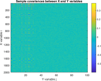
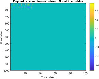
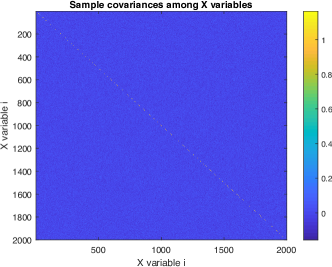
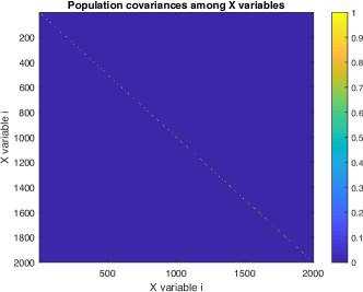
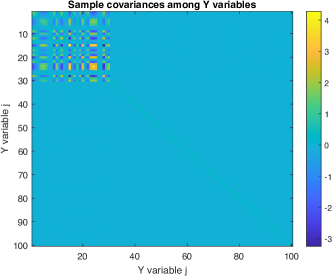
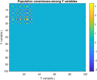
Figure S2: Experimental setup 1: Heatmaps showing the sample (left) and population (right) cross-covariances between $X$ and $Y$ variables (top), auto-covariances within $X$ variables (middle), and auto-covariances within $Y$ variables (bottom).

D-A2 Experimental setup 2: grouped variables

The population cross- and auto-covariance matrices among random vectors $\mathbf{x}$ and $\mathbf{y}$ are

$$\mathop{{\rm\mathbb{E}}}\left[\mathbf{x}\right]=\mathbf{0},\quad\mathop{{\rm\mathbb{E}}}\left[\mathbf{y}\right]=\mathbf{0}$$

$$\mathbf{\Sigma}_{\mathbf{xx}} =\mathop{{\rm\mathbb{E}}}\left[\mathbf{x}\mathbf{x}^{\rm T}\right]=\begin{bmatrix}\mathbf{\Sigma}_{1}&&&&&\\ &\ddots&&&&\\ &&\mathbf{\Sigma}_{R}&&&\\ &&&\mathbf{\Sigma}_{R+1}&&\\ &&&&\ddots&\\ &&&&&\mathbf{\Sigma}_{G}\\ \end{bmatrix}$$ (107)

$$\mathbf{\Sigma}_{\mathbf{yy}} =\mathop{{\rm\mathbb{E}}}\left[\mathbf{y}\mathbf{y}^{\rm T}\right]=c^{2}\mathbf{d}\mathbf{d}^{\rm T}+\sigma^{2}\mathbf{I}_{q}$$ (108)

$$\mathbf{\Sigma}_{\mathbf{xy}} =\mathop{{\rm\mathbb{E}}}\left[\mathbf{x}\mathbf{y}^{\rm T}\right]=\mathbf{\Sigma}_{\mathbf{xx}}\mathbf{c}\mathbf{d}^{\rm T}$$ (109)

where $\mathbf{\Sigma}_{g}=(\sigma_{gij})\in{}^{p_{g}\times p_{g}}$, with $\sigma_{gii}=1$ and $\sigma_{gij}\rho_{gi}\rho_{gj}$ for any $i\neq j$ and $g=1,2,\dots,G$, and $c^{2}\coloneqq\mathop{{\rm\mathbb{E}}}\left[z^{2}\right]=\mathbf{c}^{\rm T}\mathbf{\Sigma}_{\mathbf{xx}}\mathbf{c}$. Here $R$ is the number of relevant/informative groups.

TABLE S1: Group sizes of variables in $\mathbf{x}$

Group ID	G1	G2	G3	G4	G5	G6	G7	G8	G9	G10	G11	G12	G13	G14	G15	G16	G17	G18	G19	G20
Group size	89	112	92	88	88	99	130	103	94	91	99	91	90	112	96	100	96	91	103	100

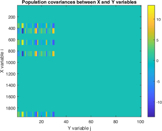
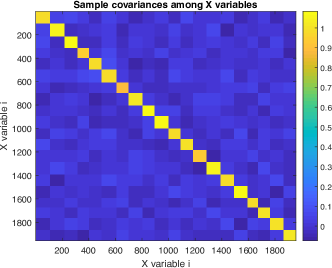
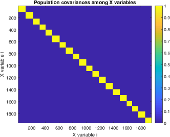
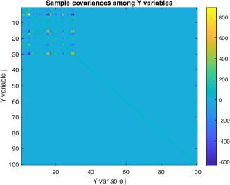
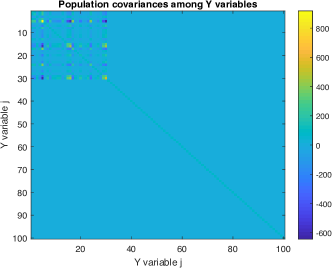
Figure S3: Experimental setup 2: Heatmaps showing the sample (left) and population (right) cross-covariances between $X$ and $Y$ variables (top), auto-covariances within $X$ variables (middle), and auto-covariances within $Y$ variables (bottom).

D-B Hyperparameter tuning and performance estimation

To select the regularization parameters $\left(c_{1},c_{2}\right)$ and estimate the generalization performance, we partition the data into training (50%, $n_{s}$ samples), validation (25%, $n_{v}$ samples), and testing (25%, $n_{t}=n-n_{s}-n_{v}$ samples) data sets:

$$\begin{bmatrix}\mathbf{X}&\mathbf{Y}\end{bmatrix}=\begin{bmatrix}\mathbf{X}_{\rm train}&\mathbf{Y}_{\rm train}\\ \mathbf{X}_{\rm val}&\mathbf{Y}_{\rm val}\\ \mathbf{X}_{\rm test}&\mathbf{Y}_{\rm test}\end{bmatrix}\in{}^{(n_{s}+n_{v}+n_{t})\times(p+q)}$$

The training and validation data are used to tune the regularization parameters $\left(c_{1},c_{2}\right)$, and the test data is used to estimate the performance.

To select the regularization parameters $\left(c_{1},c_{2}\right)$, we fit the (simplified) SCCA model on the training data using each candidate value of $\left(c_{1},c_{2}\right)$ as the regularization parameters, where $c_{1}$ and $c_{2}$ are chosen from a sequence of values equally spaced on the log scale: $c_{1}\in 2.\operatorname{\raisebox{4.30554pt}{$\scriptstyle\wedge$}}{\left(\lfloor\log_{2}c_{1,{\rm min}}\rfloor:\lceil\log_{2}c_{1,{\rm max}}\rceil\right)}$, $c_{2}\in\in 2.\operatorname{\raisebox{4.30554pt}{$\scriptstyle\wedge$}}{\left(\lfloor\log_{2}c_{2,{\rm min}}\rfloor:\lceil\log_{2}c_{2,{\rm max}}\rceil\right)}$. Here, $c_{\ell,{\rm min}}$ and $c_{\ell,{\rm max}}$, $\ell=1,2$, are the minimum and maximum value of $c_{\ell}$ which will be calculated for the standard and simplified SCCA models in Section D-B1.

Denote the solution of the model fitted with $\left(c_{1},c_{2}\right)$ as $\left(\mathbf{\hat{u}}_{\rm train}\left(c_{1},c_{2}\right),\mathbf{\hat{v}}_{\rm train}\left(c_{1},c_{2}\right)\right)$. For the standard SCCA model, the optimal $\left(c_{1},c_{2}\right)$ are chosen as

$$\left(c_{1}^{\rm opt},c_{2}^{\rm opt}\right) =\operatorname*{argmax}_{c_{1},c_{2}}\;\mathop{{\rm Corr}}\left(\mathbf{X}_{\rm val}\mathbf{\hat{u}}_{\rm train},\mathbf{Y}_{\rm val}\mathbf{\hat{v}}_{\rm train}\right)$$ (110)

$$=\operatorname*{argmax}_{c_{1},c_{2}}\;\frac{\left\langle\mathbf{X}_{\rm val}\mathbf{\hat{u}}_{\rm train},\mathbf{Y}_{\rm val}\mathbf{\hat{v}}_{\rm train}\right\rangle}{\left\|\mathbf{X}_{\rm val}\mathbf{\hat{u}}_{\rm train}\right\|\left\|\mathbf{Y}_{\rm val}\mathbf{\hat{v}}_{\rm train}\right\|}$$ (111)

For the simplified SCCA model, the optimal $\left(c_{1},c_{2}\right)$ are chosen as

$$\left(c_{1}^{\rm opt},c_{2}^{\rm opt}\right) =\operatorname*{argmax}_{c_{1},c_{2}}\;\mathop{{\rm Cov}}\left(\mathbf{X}_{\rm val}\mathbf{\hat{u}}_{\rm train}/\left\|\mathbf{\hat{u}}_{\rm train}\right\|,\mathbf{Y}_{\rm val}\mathbf{\hat{v}}_{\rm train}/\left\|\mathbf{\hat{v}}_{\rm train}\right\|\right)$$ (112)

$$=\operatorname*{argmax}_{c_{1},c_{2}}\;\frac{1}{n_{t}}\frac{\left\langle\mathbf{X}_{\rm val}\mathbf{\hat{u}}_{\rm train},\mathbf{Y}_{\rm val}\mathbf{\hat{v}}_{\rm train}\right\rangle}{\left\|\mathbf{\hat{u}}_{\rm train}\right\|\left\|\mathbf{\hat{v}}_{\rm train}\right\|}$$ (113)

Then, we refit the SCCA model with $\left(c_{1}^{\rm opt},c_{2}^{\rm opt}\right)$ on all training data (combined training and validation data) to get the solution $\left(\mathbf{\hat{u}}_{\rm trainval},\mathbf{\hat{v}}_{\rm trainval}\right)$. The canonical covariance and correlation on the test data are reported as the generalization performance:

$$\mathop{{\rm Cov}}\left(\mathbf{X}_{\rm test}\mathbf{\hat{u}}_{\rm trainval},\mathbf{Y}_{\rm test}\mathbf{\hat{v}}_{\rm trainval}\right)=\frac{\left\langle\mathbf{X}_{\rm test}\mathbf{\hat{u}}_{\rm trainval},\mathbf{Y}_{\rm test}\mathbf{\hat{v}}_{\rm trainval}\right\rangle}{\left\|\mathbf{\hat{u}}_{\rm trainval}\right\|\left\|\mathbf{\hat{v}}_{\rm trainval}\right\|}$$ (114)

$$\mathop{{\rm Corr}}\left(\mathbf{X}_{\rm test}\mathbf{\hat{u}}_{\rm trainval},\mathbf{Y}_{\rm test}\mathbf{\hat{v}}_{\rm trainval}\right)=\frac{\left\langle\mathbf{X}_{\rm test}\mathbf{\hat{u}}_{\rm trainval},\mathbf{Y}_{\rm test}\mathbf{\hat{v}}_{\rm trainval}\right\rangle}{\left\|\mathbf{X}_{\rm test}\mathbf{\hat{u}}_{\rm trainval}\right\|\left\|\mathbf{Y}_{\rm test}\mathbf{\hat{v}}_{\rm trainval}\right\|}$$ (115)

D-B1 Effective range of $c_{1}$ and $c_{2}$

To determine the range for the parameters $\left(c_{1},c_{2}\right)$ for the standard SCCA model (1), we replace its L2 inequality constraints with the L2 equality constraints:

$$\underset{\mathbf{u},\mathbf{v}}{\text{maximize}} \mathbf{u}^{\rm T}\mathbf{X}^{\rm T}\mathbf{Y}\mathbf{v}$$ (116)

subject to $$\mathbf{u}^{\rm T}\mathbf{X}^{\rm T}\mathbf{X}\mathbf{u}=1,\left\|\mathbf{u}\right\|_{1}\leq c_{1}$$

$$\mathbf{v}^{\rm T}\mathbf{Y}^{\rm T}\mathbf{Y}\mathbf{v}=1,\left\|\mathbf{v}\right\|_{1}\leq c_{2}$$

We note that for valid L1 regularization, the L1 inequality constraints needs to be active (i.e., satisfied as equalities) at the optimal solution. This implies that

$$c_{1}\geq\underset{\mathbf{u}}{\text{minimize}}\;\left\|\mathbf{u}\right\|_{1}\quad\text{subject to }\left\|\mathbf{X}\mathbf{u}\right\|^{2}=1$$ (117)

$$c_{2}\geq\underset{\mathbf{v}}{\text{minimize}}\;\left\|\mathbf{v}\right\|_{1}\quad\text{subject to }\left\|\mathbf{Y}\mathbf{v}\right\|^{2}=1$$ (118)

and

$$c_{1}\leq\underset{\mathbf{u}}{\text{maximize}}\;\left\|\mathbf{u}\right\|_{1}\quad\text{subject to }\left\|\mathbf{X}\mathbf{u}\right\|^{2}=1$$ (119)

$$c_{2}\leq\underset{\mathbf{v}}{\text{maximize}}\;\left\|\mathbf{v}\right\|_{1}\quad\text{subject to }\left\|\mathbf{Y}\mathbf{v}\right\|^{2}=1$$ (120)

Simple analysis shows that a sufficient condition for (117)-(118) to hold is

$$c_{1}\geq\mathop{{\rm max}}\left(\frac{1}{{\color[rgb]{0,0,0}{{\sigma_{\rm max}}}}\left(\mathbf{X}\right)},\frac{1}{\sqrt{\sum_{\ell=1}^{n}\max_{1\leq i\leq p}x_{\ell i}^{2}}}\right)\eqqcolon c_{1,{\rm min}}$$ (121)

$$c_{2}\geq\mathop{{\rm max}}\left(\frac{1}{{\color[rgb]{0,0,0}{{\sigma_{\rm max}}}}\left(\mathbf{Y}\right)},\frac{1}{\sqrt{\sum_{\ell=1}^{n}\max_{1\leq j\leq q}y_{\ell j}^{2}}}\right)\eqqcolon c_{2,{\rm min}}$$ (122)

Note however, that the objective in (119) (resp., (120)) is unbounded above when $n<p$ (resp., $n<q$), and thus it can not be used to find an effective maximum of $c_{1}$ (resp., $c_{2}$). To find an effective maximum value of $c_{1}$ and $c_{2}$, we solve problem (116) in the absence of L1 constraints instead:

$$\underset{\mathbf{u},\mathbf{v}}{\text{maximize}} \mathbf{u}^{\rm T}\mathbf{X}^{\rm T}\mathbf{Y}\mathbf{v}$$ (123)

subject to $$\mathbf{u}^{\rm T}\mathbf{X}^{\rm T}\mathbf{X}\mathbf{u}=1$$

$$\mathbf{v}^{\rm T}\mathbf{Y}^{\rm T}\mathbf{Y}\mathbf{v}=1$$

Denote the optimal solution of problem 123 as $\left(\mathbf{u}^{*},\mathbf{v}^{*}\right)$. We set $c_{1,{\rm max}}=\left\|\mathbf{u}^{*}\right\|_{1}$ and $c_{2,{\rm max}}=\left\|\mathbf{v}^{*}\right\|_{1}$.

It can be shown that $\mathbf{u}^{*}=\left(\mathbf{X}^{\rm T}\mathbf{X}\right)^{-1/2}\mathbf{u}_{1},\mathbf{v}^{*}=\left(\mathbf{Y}^{\rm T}\mathbf{Y}\right)^{-1/2}\mathbf{v}_{1}$, where $\mathbf{u}_{1}$ and $\mathbf{v}_{1}$ are respectively the left and right singular vectors of $\left(\mathbf{X}^{\rm T}\mathbf{X}\right)^{-1/2}\mathbf{X}^{\rm T}\mathbf{Y}\left(\mathbf{Y}^{\rm T}\mathbf{Y}\right)^{-1/2}$ associated with the largest singular value. If $\mathbf{X}^{\rm T}\mathbf{X}$ is singular, we can use $\mathbf{X}^{\rm T}\mathbf{X}+\epsilon\mathbf{I}_{p}$ to approximate it; likewise for $\mathbf{Y}^{\rm T}\mathbf{Y}$.

In a similar line of reasoning, to determine the range for the parameters $\left(c_{1},c_{2}\right)$ for the simplified SCCA model (1), consider

$$\underset{\mathbf{u},\mathbf{v}}{\text{maximize}} \mathbf{u}^{\rm T}\mathbf{X}^{\rm T}\mathbf{Y}\mathbf{v}$$ (124)

subject to $$\left\|\mathbf{u}\right\|^{2}=1,\left\|\mathbf{u}\right\|_{1}\leq c_{1}$$

$$\left\|\mathbf{v}\right\|^{2}=1,\left\|\mathbf{v}\right\|_{1}\leq c_{2}$$

We note that an effective value of $c_{1}$ and $c_{2}$ should be such that the L1 inequality constraints are active (i.e., satisfied as equalities) at the optimal solution.

To this end, it should satisfy

$$c_{1}\geq\underset{\mathbf{u}}{\text{minimize}}\;\left\|\mathbf{u}\right\|_{1}\quad\text{subject to }\left\|\mathbf{u}\right\|^{2}=1$$ (125)

$$c_{2}\geq\underset{\mathbf{v}}{\text{minimize}}\;\left\|\mathbf{v}\right\|_{1}\quad\text{subject to }\left\|\mathbf{v}\right\|^{2}=1$$ (126)

and

$$c_{1}\leq\underset{\mathbf{u}}{\text{maximize}}\;\left\|\mathbf{u}\right\|_{1}\quad\text{subject to }\left\|\mathbf{u}\right\|^{2}=1$$ (127)

$$c_{2}\leq\underset{\mathbf{v}}{\text{maximize}}\;\left\|\mathbf{v}\right\|_{1}\quad\text{subject to }\left\|\mathbf{v}\right\|^{2}=1$$ (128)

From (125)-(128), it follows that

$$c_{1,{\rm min}}\coloneqq 1\leq c_{1}\leq\sqrt{p}$$ (129)

$$c_{2,{\rm min}}\coloneqq 1\leq c_{2}\leq\sqrt{q}$$ (130)

The upper bounds $\sqrt{p}$ for $c_{1}$ and $\sqrt{q}$ for $c_{2}$ are too relaxed. To find a tighter bound, we solve problem (124) in the absence of L1 constraints instead:

$$\underset{\mathbf{u},\mathbf{v}}{\text{maximize}} \mathbf{u}^{\rm T}\mathbf{X}^{\rm T}\mathbf{Y}\mathbf{v}$$ (131)

subject to $$\left\|\mathbf{u}\right\|^{2}=1$$

$$\left\|\mathbf{v}\right\|^{2}=1$$

The optimal solution is $\mathbf{u}^{*}=\mathbf{u}_{1},\mathbf{v}^{*}=\mathbf{v}_{1}$, where $\mathbf{u}_{1}$ and $\mathbf{v}_{1}$ are respectively the left and right singular vectors of $\mathbf{X}^{\rm T}\mathbf{Y}$ associated with the largest singular value. We set $c_{1,{\rm max}}=\left\|\mathbf{u}^{*}\right\|_{1}$ and $c_{2,{\rm max}}=\left\|\mathbf{v}^{*}\right\|_{1}$.

D-C Variable selection performance

The balanced accuracy (bACC) and Matthews correlation coefficient (MCC) are defined as

$$\mathrm{bACC}=\frac{1}{2}\left(\frac{\mathrm{TP}}{\mathrm{TP}+\mathrm{FN}}+\frac{\mathrm{TN}}{\mathrm{TN}+\mathrm{FP}}\right),$$ (132)

$$\mathrm{MCC}=\frac{\mathrm{TP}\times\mathrm{TN}-\mathrm{FP}\times\mathrm{FN}}{\sqrt{(\mathrm{TP}+\mathrm{FP})(\mathrm{TP}+\mathrm{FN})(\mathrm{TN}+\mathrm{FP})(\mathrm{TN}+\mathrm{FN})}},$$ (133)

where TP, TN, FP, and FN denote the numbers of true positives, true negatives, false positives, and false negatives, respectively. The bACC and MCC are overall measures of variable selection accuracy, and a larger score indicates a better variable selection performance.The relative absolute error (RAE), which for the selection of $X$ variables is defined as

$$\mathrm{RAE}=\frac{\left\|\mathbf{\hat{u}}-\mathbf{u}^{*}\right\|_{1}}{\left\|\mathbf{u}^{*}\right\|_{1}}$$ (134)

where $\mathbf{u}^{*}$ and $\mathbf{\hat{u}}$ denote the true and estimated canonical vector, respectively. Our variable selection performance on the synthetic data is shown in Table S2 and Table S3.

TABLE S2: The $X$ variable selection performance of the SCCA and simplified SCCA on whole training data.

Model	Recall	Precision	F1 score	ACC	bACC	MCC	PR AUC	RAE
Experimental setup 1
SCCA	0.820	0.276	0.413	0.767	0.791	0.382	0.759	0.384
Simp SCCA	0.430	0.306	0.358	0.846	0.661	0.278	0.429	1.044
Experimental setup 2
SCCA	1.000	0.233	0.378	0.233	0.500	NaN	0.998	0.320
Simp SCCA	1.000	0.602	0.751	0.846	0.899	0.693	0.800	0.110

TABLE S3: The $Y$ variable selection performance of the SCCA and simplified SCCA on whole training data.

Model	Recall	Precision	F1 score	ACC	bACC	MCC	PR AUC	RAE
Experimental setup 1
SCCA	1.000	0.300	0.462	0.300	0.500	NaN	0.896	0.823
Simp SCCA	1.000	0.566	0.723	0.770	0.836	0.616	0.957	0.030
Experimental setup 2
SCCA	1.000	0.300	0.462	0.300	0.500	NaN	0.844	0.503
Simp SCCA	0.967	0.558	0.707	0.760	0.819	0.585	0.948	0.050

Appendix E Supporting Information and additional results for imaging genetic data analysis in Section (V-B)

E-A Subject characteristics

TABLE S4: Subject characteristics

	HC	SMC	EMCI	LMCI	AD
Num	183	75	218	184	97
Gender (M/F)	89/94	29/46	113/105	96/88	54/43
Handedness (R/L)	163/20	65/10	195/23	165/19	89/8
Age (mean$\pm$std)	73.96$\pm$5.50	71.77$\pm$5.76	70.56$\pm$7.16	71.89$\pm$7.92	73.99$\pm$8.44
Edu (mean$\pm$std)	16.44$\pm$2.67	16.87$\pm$2.71	15.95$\pm$2.64	16.14$\pm$2.92	15.60$\pm$2.61

Participant characteristics of our real imaging genetics data from the Alzheimer’s Disease Neuroimaging Initiative (ADNI) cohort is shown in Table S4.

E-B Correlation structure of the real imaging genetic data

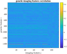
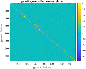
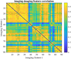
Figure S4: Heatmaps showing the pairwise sample Pearson correlation coefficients between genetic and imaging features (left), within genetic features (middle), and within imaging features (right).

Correlation structure of the real ADNI imaging genetics data used in this study is shown in Fig. S4.

E-C Hyperparameter tuning and generalization performance estimation

We employ the nested cross-validation method which is an extension of the procedure described in Section D-B. We first randomly divide each category of subjects into five roughly equal-sized subgroups and combine the data from each category to form five outer folds.

We used the first fold for testing and the remaining folds for training/validating the model. Test set data are put aside. The following steps were carried out with the training+validation data:

(1)

We employ the stratified cross-validation (CV) method to choose $\left(c_{1},c_{2}\right)$. The samples/subjects from each category are randomly divided into five roughly equal-sized subgroups and then combined to form five folds ${\mathcal{I}}=\cup_{k=1}^{5}{\mathcal{I}}_{k}$. Denote $\mathbf{X}_{{\mathcal{I}}_{k}}^{\rm trainval}$ and $\mathbf{Y}_{{\mathcal{I}}_{k}}^{\rm trainval}$, $k=1,2,\dots,5$, as the submatrices formed by the rows of $\mathbf{X}^{\rm trainval}$ and $\mathbf{Y}^{\rm trainval}$ indexed by ${\mathcal{I}}_{k}$, respectively.

(2)

The SCCA model is fitted to the normalized $\left(\mathbf{X}_{{\mathcal{I}}\setminus{\mathcal{I}}_{1}}^{\rm trainval},\mathbf{Y}_{{\mathcal{I}}\setminus{\mathcal{I}}_{1}}^{\rm trainval}\right)$ to obtain the solution as $\left(\mathbf{\hat{u}}_{-1}^{\rm trainval},\mathbf{\hat{v}}_{-1}^{\rm trainval}\right)$. Then, the performance on the validation data is recorded as $\mathop{{\rm Corr}}\left(\mathbf{X}_{{\mathcal{I}}_{1}}^{\rm trainval}\mathbf{\hat{u}}_{-1}^{\rm trainval},\mathbf{Y}_{{\mathcal{I}}_{1}}^{\rm trainval}\mathbf{\hat{v}}_{-1}^{\rm trainval}\right)$. This process is repeated five times with each fold of samples/subjects used once as the validation set.

(3)

The cross-validation criterion to select the regularization parameters is defined as

$$\left(c_{1}^{\rm opt},c_{2}^{\rm opt}\right)=\operatorname*{argmax}_{c_{1},c_{2}}\;\frac{1}{5}\sum_{k=1}^{5}\mathop{{\rm Corr}}\left(\mathbf{X}_{{\mathcal{I}}_{k}}^{\rm trainval}\mathbf{\hat{u}}_{-k}^{\rm trainval},\mathbf{Y}_{{\mathcal{I}}_{k}}^{\rm trainval}\mathbf{\hat{v}}_{-k}^{\rm trainval}\right)$$ (135)

where $\mathop{{\rm Corr}}\left(\cdot,\cdot\right)$ is the correlation function and $\left(\mathbf{\hat{u}}_{-k}^{\rm trainval},\mathbf{\hat{v}}_{-k}^{\rm trainval}\right)$ are the estimates of $\left(\mathbf{u},\mathbf{v}\right)$ by the standard SCCA on the training+validation data $\left(\mathbf{X}_{{\mathcal{I}}\setminus{\mathcal{I}}_{k}}^{\rm trainval},\mathbf{Y}_{{\mathcal{I}}\setminus{\mathcal{I}}_{k}}^{\rm trainval}\right)$ with $\left(c_{1},c_{2}\right)$ as regularization parameters.

(4)

The SCCA model was then fit to the entire training set at $\left(c_{1}^{\rm opt},c_{2}^{\rm opt}\right)$ to estimate the canonical weights $\left(\mathbf{\hat{u}}^{\rm opt},\mathbf{\hat{v}}^{\rm opt}\right)$.

The canonical correlation on the test data $\mathop{{\rm Corr}}\left(\mathbf{X}_{\rm test}\mathbf{\hat{u}}^{\rm opt},\mathbf{Y}_{\rm test}\mathbf{\hat{v}}^{\rm opt}\right)$ is reported as the generalization performance. For the simplified SCCA, the canonical covariance is used as the metric to measure the performance and to tune the regularization parameters.

This process is repeated five times with each outer fold of samples/subjects used once as the testing set.

E-D Genetic and Imaging Marker Selection

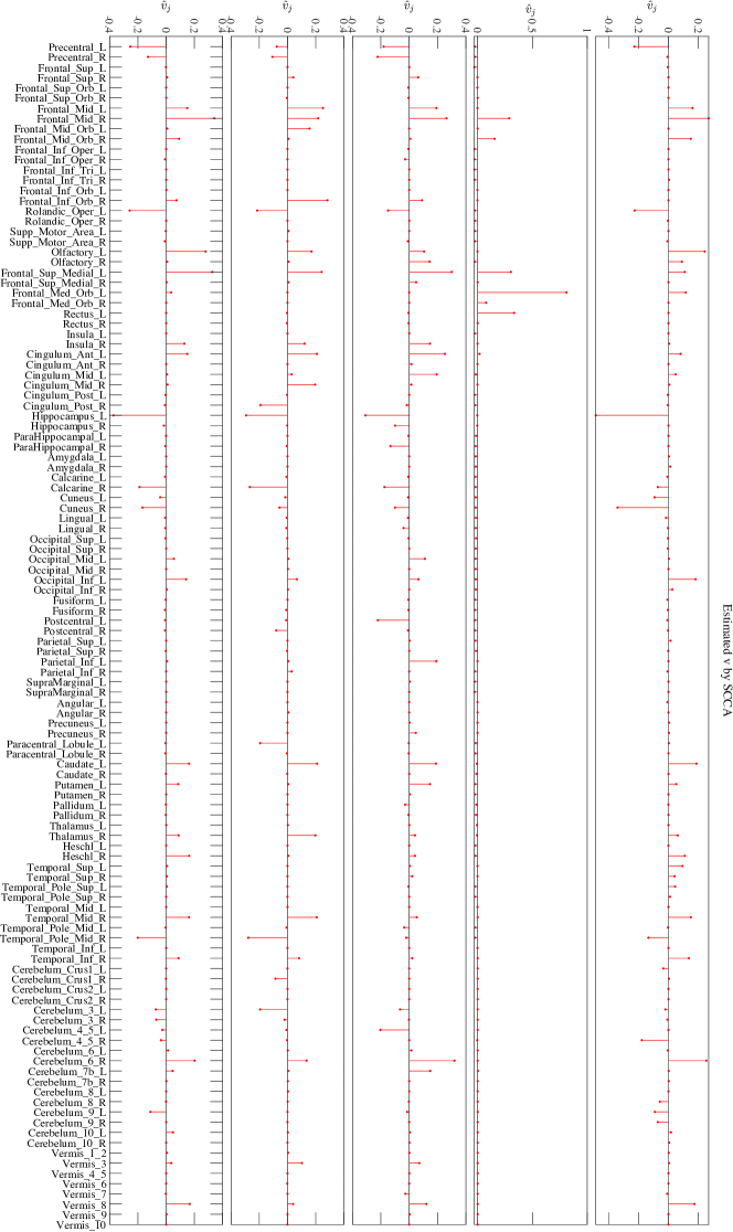
Figure S6: Canonical imaging weights estimated by SCCA (top figure) and simplified SCCA (bottom figure). In each figure, the results on each of the four training folds (rows 1-4) and on the entire data (bottom row) are shown.

TABLE S5: Genetic features (ordered by absolute values of estimated canonical weights) selected by SCCA and simplified SCCA.

Standard SCCA				Simplified SCCA
SNP	Closest gene	$\hat{u}_{i}$	p-value	SNP	Closest gene	$\hat{u}_{i}$	p-value
rs4420638	APOE	0.892	8.50e-12	rs4420638	APOE	0.522	8.50e-12
rs769449	APOE	0.366	1.60e-12	rs769449	APOE	0.466	1.60e-12
rs10404947	ABCA7	0.140	5.16e-02	rs157582	APOE	0.408	2.37e-05
rs12434016	SLC24A4	-0.102	9.11e-01	rs2075650	APOE	0.383	4.46e-07
rs17258982	CR1	0.069	5.83e-01	rs1160985	APOE	-0.213	7.29e-06
rs609903	PICALM	-0.065	6.38e-01	rs8106922	APOE	-0.183	2.27e-03
rs7141622	RIN3	0.058	8.92e-01	rs6859	APOE	0.156	9.20e-03
rs3818361	CR1	0.056	8.24e-03	rs405509	APOE	-0.121	4.20e-03
rs923892	SORL1	-0.052	3.82e-01	rs157580	APOE	-0.111	1.70e-01
rs2949766	EPHA1	0.051	1.58e-01	rs584007	APOE	-0.084	3.85e-01
rs17126012	FERMT2	0.048	4.25e-01	rs439401	APOE	-0.078	3.26e-01
rs3087554	CLU	0.046	4.43e-01	rs10404947	ABCA7	0.076	5.16e-02
rs1160985	APOE	-0.043	7.29e-06	rs609903	PICALM	-0.067	6.38e-01
rs6843	ABCA7	0.043	1.61e-01	rs637304	PICALM	-0.067	3.06e-01
rs1422189	MEF2C	-0.042	5.00e-02	rs6843	ABCA7	0.066	1.61e-01
rs2304607	MEF2C	-0.040	2.05e-01	rs519825	APOE	0.060	5.48e-01
rs17660414	DSG2	-0.038	9.48e-01	rs694011	PICALM	-0.059	5.21e-01
rs6064401	CASS4	0.035	5.46e-01	rs2074442	ABCA7	0.057	1.12e-01
rs11230197	MS4A6A	0.034	3.81e-01	rs757232	ABCA7	0.053	8.50e-02
rs93882	SORL1	0.022	4.83e-01	rs561655	PICALM	-0.050	6.54e-01
rs12703526	EPHA1	-0.022	9.19e-01	rs1237999	PICALM	-0.043	8.32e-01
rs611267	MS4A6A	-0.021	1.19e-01	rs34374273	APOE	-0.041	5.45e-02
rs7936092	PICALM	0.021	2.07e-01	rs1667284	DSG2	-0.041	6.87e-01
rs733430	SORL1	0.020	2.08e-01	rs10898436	PICALM	0.040	4.00e-01
rs2279796	ABCA7	-0.020	3.68e-01	rs11608136	PICALM	-0.040	7.11e-01
rs8008270	FERMT2	-0.013	5.49e-02	rs8013925	RIN3	0.040	5.30e-01
rs8013925	RIN3	0.012	5.30e-01	rs1791161	DSG2	-0.040	6.82e-01
rs157582	APOE	0.011	2.37e-05	rs543293	PICALM	-0.029	7.78e-01
rs1667284	DSG2	-0.009	6.87e-01	rs17258982	CR1	0.027	5.83e-01
rs4752856	CELF1	-0.009	8.21e-01	rs7143400	FERMT2	0.026	8.64e-01
rs558788	MS4A6A	-0.007	6.15e-01	rs3851179	PICALM	-0.021	8.13e-01
rs11952384	MEF2C	-0.007	5.46e-01	rs405697	APOE	-0.020	2.60e-01
rs1784927	SORL1	-0.006	2.66e-01	rs4147932	ABCA7	0.017	3.80e-01
rs4720262	NME8	0.006	8.96e-01	rs3818361	CR1	0.017	8.24e-03
rs8106922	APOE	-0.006	2.27e-03	rs12961029	DSG2	0.017	1.13e-01
rs12709651	DSG2	0.005	8.95e-01	rs8008270	FERMT2	-0.016	5.49e-02
rs244749	MEF2C	0.005	1.60e-01	rs7941541	PICALM	-0.016	7.83e-01
rs753812	CELF1	0.005	5.95e-01	rs7160582	FERMT2	0.016	8.25e-01
rs2075650	APOE	0.005	4.46e-07	rs17125944	FERMT2	0.015	4.57e-01
rs7584458	INPP5D	-0.005	4.06e-01	rs16979595	APOE	0.014	5.87e-01
rs7569827	INPP5D	-0.005	3.62e-01	rs4904920	SLC24A4	0.014	8.38e-01
rs2104239	RIN3	0.004	1.72e-02	rs2357947	FERMT2	0.014	8.50e-01
rs10742816	CELF1	0.004	5.34e-01	rs11157933	FERMT2	0.014	8.50e-01
rs4752839	CELF1	0.004	5.04e-01	rs6572869	FERMT2	0.014	8.50e-01
rs4663337	INPP5D	-0.004	3.97e-01	rs2405442	ZCWPW1	-0.013	2.75e-01
rs254778	MEF2C	0.004	8.06e-01	rs11623185	RIN3	-0.013	5.53e-01
rs1117067	MS4A6A	0.004	4.21e-01	rs2104239	RIN3	0.011	1.72e-02
rs11230193	MS4A6A	0.004	4.79e-01	rs6951852	EPHA1	-0.011	1.96e-01
rs4939319	MS4A6A	0.004	4.79e-01	rs7580869	INPP5D	-0.011	1.28e-01
rs7929057	MS4A6A	0.004	4.79e-01	rs10134832	SLC24A4	-0.009	4.92e-01
rs1866236	BIN1	0.003	1.01e-01	rs1026123	DSG2	-0.009	5.14e-01
rs11218325	SORL1	0.003	1.10e-01	rs1667280	DSG2	-0.009	5.14e-01
rs1791161	DSG2	-0.003	6.82e-01	rs12434016	SLC24A4	-0.008	9.11e-01
rs1871045	APOE	0.003	9.67e-01	rs273622	CD33	0.007	2.38e-01
rs6069767	CASS4	0.003	4.47e-01	rs660895	HLA-DRB1	0.007	6.42e-01
rs4662703	BIN1	0.003	5.21e-01	rs17729233	DSG2	-0.006	7.17e-01
rs757232	ABCA7	0.003	8.50e-02	rs12709651	DSG2	0.003	8.95e-01
rs7026	APOE	0.003	9.86e-01	rs17660414	DSG2	-0.003	9.48e-01
rs12476339	BIN1	0.003	5.53e-01	rs1710354	CD33	-0.002	2.95e-01
rs674747	MEF2C	0.002	4.33e-01	rs10413089	APOE	0.002	1.15e-01
rs4938933	MS4A6A	-0.002	3.67e-01	rs12539172	ZCWPW1	-0.002	5.44e-01
rs17186722	CR1	-0.002	5.20e-01	rs13426725	BIN1	0.000	1.20e-01
rs3752243	ABCA7	-0.002	5.98e-01	rs10779277	CR1	0.000	2.92e-01
rs2161228	MEF2C	-0.002	1.49e-01	rs2490255	CR1	0.000	2.65e-01
rs543293	PICALM	-0.002	7.78e-01	rs17186722	CR1	0.000	5.20e-01
rs3738468	CR1	-0.002	6.84e-01	rs2940252	CR1	0.000	5.18e-01
rs881768	ABCA7	-0.002	6.04e-01	rs2661361	CR1	0.000	3.76e-01
rs694011	PICALM	-0.002	5.21e-01	rs6664001	CR1	0.000	2.68e-01
rs4752845	CELF1	-0.002	8.76e-01	rs17042520	CR1	0.000	6.56e-01
rs12798346	CELF1	-0.002	8.76e-01	rs2135924	CR1	0.000	2.68e-01
rs10838738	CELF1	-0.002	8.76e-01	rs6656123	CR1	0.000	3.10e-01
rs1871047	APOE	0.002	7.06e-01	rs311299	CR1	0.000	3.73e-01
rs4726624	EPHA1	0.002	6.40e-01	rs12734973	CR1	0.000	5.06e-01
rs6951852	EPHA1	-0.001	1.96e-01	rs1032980	CR1	0.000	3.70e-01
rs17014818	BIN1	0.001	5.08e-01	rs17615	CR1	0.000	2.94e-01
rs12155159	NME8	-0.001	4.05e-01	rs4308977	CR1	0.000	4.17e-01
rs676759	SORL1	-0.001	5.51e-01	rs17616	CR1	0.000	3.40e-01
rs8018746	SLC24A4	-0.001	3.49e-01	rs7549152	CR1	0.000	5.70e-01
rs6591559	MS4A6A	-0.001	3.62e-01	rs2182909	CR1	0.000	3.73e-01
rs1530914	MS4A6A	-0.001	3.62e-01	rs6540433	CR1	0.000	5.06e-01
rs17128308	SLC24A4	0.001	1.86e-01	rs6690215	CR1	0.000	9.38e-02
rs3752242	ABCA7	-0.001	6.49e-01	rs12021671	CR1	0.000	1.26e-01
rs4904920	SLC24A4	0.001	8.38e-01	rs2182911	CR1	0.000	1.56e-01
rs3754617	BIN1	0.001	6.93e-01	rs4618970	CR1	0.000	6.50e-01
rs2722246	NME8	-0.001	9.90e-01	rs9429940	CR1	0.000	6.50e-01
rs561655	PICALM	-0.001	6.54e-01	rs11117956	CR1	0.000	1.90e-01
rs412458	MEF2C	0.001	3.16e-01	rs11117959	CR1	0.000	5.21e-01
rs7580869	INPP5D	-0.001	1.28e-01	rs10127904	CR1	0.000	2.85e-02
rs11117959	CR1	-0.001	5.21e-01	rs2274566	CR1	0.000	4.70e-02
rs12883551	SLC24A4	-0.000	2.36e-01	rs3738468	CR1	0.000	6.84e-01
rs2074442	ABCA7	0.000	1.12e-01	rs17259045	CR1	0.000	7.45e-01
rs4752993	CELF1	-0.000	8.27e-01	rs6691117	CR1	0.000	2.46e-01
rs12453	MS4A6A	-0.000	6.72e-02	rs12032275	CR1	0.000	6.76e-01
rs1237999	PICALM	-0.000	8.32e-01	rs12734030	CR1	0.000	3.09e-01
rs755553	CELF1	-0.000	8.66e-01	rs12034383	CR1	0.000	2.51e-02
rs10426423	APOE	0.000	6.63e-01	rs10779339	CR1	0.000	4.55e-01
rs7124060	SORL1	0.000	2.28e-01	rs10494885	CR1	0.000	4.65e-01
rs10779277	CR1	-0.000	2.92e-01	rs6696840	CR1	0.000	4.86e-01
rs2490255	CR1	-0.000	2.65e-01	rs1323721	CR1	0.000	2.43e-01
rs2940252	CR1	-0.000	5.18e-01	rs10863461	CR1	0.000	2.46e-01

TABLE S6: Imaging features (ordered by absolute values of estimated canonical weights) selected by SCCA and simplified SCCA.

Standard SCCA			Simplified SCCA
brain ROI	$\hat{v}_{j}$	p-value	brain ROI	$\hat{v}_{j}$	p-value
Hippocampus_L	-0.403	1.25e-08	Frontal_Med_Orb_L	0.138	9.65e-26
Frontal_Mid_R	0.279	4.84e-18	Frontal_Sup_Medial_L	0.135	8.66e-21
Frontal_Mid_L	0.261	1.67e-18	Cingulum_Ant_L	0.133	2.32e-19
Precentral_L	-0.249	7.67e-07	Frontal_Med_Orb_R	0.133	1.04e-24
Rolandic_Oper_L	-0.238	4.63e-10	Frontal_Sup_Medial_R	0.132	4.47e-20
Frontal_Sup_Medial_L	0.235	8.66e-21	Rectus_L	0.132	3.33e-25
Cerebelum_6_R	0.219	5.71e-10	Frontal_Mid_R	0.130	4.84e-18
Calcarine_R	-0.216	5.11e-13	Frontal_Mid_Orb_R	0.129	5.09e-21
Insula_R	0.206	1.67e-16	Frontal_Mid_L	0.129	1.67e-18
Cingulum_Ant_L	0.188	2.32e-19	Temporal_Mid_R	0.128	2.15e-20
Temporal_Pole_Mid_R	-0.187	1.39e-06	Rectus_R	0.128	4.53e-22
Caudate_L	0.185	1.38e-01	Frontal_Sup_Orb_R	0.128	3.23e-20
Precentral_R	-0.179	1.25e-05	Insula_R	0.127	1.67e-16
Vermis_8	0.171	9.35e-01	Temporal_Inf_R	0.127	6.79e-19
Temporal_Inf_R	0.169	6.79e-19	Frontal_Sup_Orb_L	0.127	7.41e-20
Cuneus_R	-0.165	9.59e-07	Frontal_Mid_Orb_L	0.126	3.34e-21
Olfactory_L	0.130	1.46e-13	Frontal_Inf_Orb_R	0.126	2.57e-14
Heschl_R	0.130	6.06e-17	Olfactory_L	0.125	1.46e-13
Occipital_Inf_L	0.112	2.30e-13	Cingulum_Mid_L	0.125	8.86e-22
Cerebelum_9_L	-0.112	1.18e-03	Cingulum_Mid_R	0.125	2.12e-19
Thalamus_R	0.108	9.22e-01	Frontal_Inf_Orb_L	0.124	1.64e-17
Cerebelum_3_L	-0.107	2.41e-05	Cingulum_Ant_R	0.123	6.76e-15
Putamen_L	0.105	2.11e-17	Frontal_Sup_R	0.123	1.35e-14
Frontal_Med_Orb_L	0.098	9.65e-26	Temporal_Sup_R	0.123	2.06e-20
Temporal_Mid_R	0.097	2.15e-20	Temporal_Mid_L	0.121	1.94e-21
Occipital_Mid_L	0.090	1.55e-09	Precuneus_L	0.121	8.66e-22
Frontal_Inf_Orb_R	0.081	2.57e-14	Olfactory_R	0.120	7.48e-11
Frontal_Mid_Orb_R	0.073	5.09e-21	Precuneus_R	0.120	8.93e-23
Olfactory_R	0.069	7.48e-11	Frontal_Inf_Tri_L	0.120	4.56e-16
Vermis_3	0.059	1.05e-01	Temporal_Inf_L	0.119	5.09e-19
Cerebelum_3_R	-0.053	1.33e-05	Temporal_Sup_L	0.119	8.89e-17
Cerebelum_4_5_R	-0.052	5.88e-09	Frontal_Sup_L	0.119	6.30e-15
Cuneus_L	-0.052	5.56e-06	Parietal_Inf_L	0.119	2.94e-15
Frontal_Sup_R	0.051	1.35e-14	SupraMarginal_R	0.118	7.04e-15
Cerebelum_10_L	0.044	1.02e-04	Frontal_Inf_Tri_R	0.117	4.50e-13
Cerebelum_7b_L	0.042	4.67e-07	Angular_R	0.117	5.56e-16
Hippocampus_R	-0.034	4.66e-08	Angular_L	0.116	6.30e-17
Cerebelum_4_5_L	-0.033	1.29e-04	Parietal_Inf_R	0.115	7.79e-14
Cerebelum_6_L	0.032	1.69e-09	Insula_L	0.115	4.36e-14
Cingulum_Mid_R	0.023	2.12e-19	Heschl_R	0.114	6.06e-17
Supp_Motor_Area_R	-0.010	7.83e-15	SupraMarginal_L	0.113	2.29e-11
Cingulum_Post_R	-0.009	3.18e-04	Frontal_Inf_Oper_R	0.112	2.22e-14
Fusiform_R	-0.009	1.94e-20	Rolandic_Oper_R	0.111	2.84e-13
Postcentral_L	-0.009	2.91e-09	Supp_Motor_Area_L	0.110	1.13e-15
Frontal_Mid_Orb_L	0.008	3.34e-21	Fusiform_R	0.110	1.94e-20
Postcentral_R	-0.008	1.85e-08	Cingulum_Post_L	0.108	5.66e-13
Calcarine_L	-0.008	3.33e-17	Fusiform_L	0.108	4.12e-19
Frontal_Inf_Oper_R	-0.008	2.22e-14	Frontal_Inf_Oper_L	0.106	4.89e-12
Lingual_L	-0.008	2.68e-15	Putamen_L	0.106	2.11e-17
Cingulum_Mid_L	0.007	8.86e-22	Putamen_R	0.106	4.16e-15
Parietal_Inf_L	0.007	2.94e-15	Heschl_L	0.105	1.05e-14
Frontal_Sup_Medial_R	0.007	4.47e-20	Temporal_Pole_Sup_L	0.104	3.30e-08
Temporal_Sup_L	0.007	8.89e-17	Temporal_Pole_Sup_R	0.104	4.33e-09
ParaHippocampal_R	-0.007	4.46e-01	Occipital_Mid_L	0.101	1.55e-09
Temporal_Sup_R	0.006	2.06e-20	Occipital_Inf_L	0.100	2.30e-13
Paracentral_Lobule_R	-0.006	3.84e-12	Supp_Motor_Area_R	0.098	7.83e-15
Lingual_R	-0.006	7.85e-17	Rolandic_Oper_L	0.095	4.63e-10
Temporal_Pole_Sup_L	0.005	3.30e-08	Parietal_Sup_L	0.094	3.29e-10
Paracentral_Lobule_L	-0.005	5.85e-08	Temporal_Pole_Mid_L	0.093	2.11e-07
Vermis_1_2	0.005	6.11e-04	Occipital_Mid_R	0.092	1.56e-08
Occipital_Sup_L	-0.005	1.43e-02	Occipital_Inf_R	0.091	1.26e-09
Occipital_Inf_R	0.005	1.26e-09	Calcarine_L	0.091	3.33e-17
Cingulum_Post_L	-0.004	5.66e-13	Temporal_Pole_Mid_R	0.088	1.39e-06
Temporal_Pole_Mid_L	-0.004	2.11e-07	Postcentral_R	0.087	1.85e-08
Fusiform_L	-0.004	4.12e-19	Postcentral_L	0.086	2.91e-09
Pallidum_R	-0.004	3.78e-03	Paracentral_Lobule_R	0.084	3.84e-12
Parietal_Sup_R	-0.003	3.11e-05	Lingual_R	0.081	7.85e-17
Pallidum_L	-0.002	4.55e-02	Precentral_L	0.078	7.67e-07
Caudate_R	-0.002	5.42e-01	Lingual_L	0.078	2.68e-15
Vermis_9	0.002	9.51e-02	Amygdala_L	0.078	8.42e-07
Vermis_7	-0.002	4.63e-02	Cingulum_Post_R	0.076	3.18e-04
Cerebelum_Crus1_R	-0.002	3.23e-03	Precentral_R	0.074	1.25e-05
Cerebelum_8_R	-0.001	3.11e-06	Amygdala_R	0.073	1.09e-02
Cerebelum_7b_R	0.001	6.70e-05	Calcarine_R	0.072	5.11e-13
Frontal_Inf_Oper_L	-0.001	4.89e-12	Parietal_Sup_R	0.071	3.11e-05
Frontal_Inf_Orb_L	0.001	1.64e-17	Cuneus_L	0.071	5.56e-06
ParaHippocampal_L	-0.001	4.57e-01	Paracentral_Lobule_L	0.068	5.85e-08
Thalamus_L	0.001	2.74e-01	Occipital_Sup_R	0.067	4.50e-05
Supp_Motor_Area_L	-0.000	1.13e-15	ParaHippocampal_R	0.064	4.46e-01
Frontal_Sup_L	-0.000	6.30e-15	Cerebelum_6_R	0.062	5.71e-10
Frontal_Sup_Orb_L	-0.000	7.41e-20	Occipital_Sup_L	0.059	1.43e-02
Frontal_Sup_Orb_R	-0.000	3.23e-20	Cuneus_R	0.059	9.59e-07
Frontal_Inf_Tri_L	-0.000	4.56e-16	Caudate_R	0.057	5.42e-01
Frontal_Inf_Tri_R	-0.000	4.50e-13	Pallidum_R	0.056	3.78e-03
Rolandic_Oper_R	-0.000	2.84e-13	Caudate_L	0.054	1.38e-01
Frontal_Med_Orb_R	-0.000	1.04e-24	Cerebelum_6_L	0.051	1.69e-09
Rectus_L	-0.000	3.33e-25	ParaHippocampal_L	0.051	4.57e-01
Rectus_R	-0.000	4.53e-22	Pallidum_L	0.047	4.55e-02
Insula_L	-0.000	4.36e-14	Cerebelum_3_L	-0.044	2.41e-05
Cingulum_Ant_R	-0.000	6.76e-15	Cerebelum_8_R	-0.042	3.11e-06
Amygdala_L	-0.000	8.42e-07	Cerebelum_8_L	-0.042	2.15e-05
Amygdala_R	-0.000	1.09e-02	Cerebelum_4_5_R	0.041	5.88e-09
Occipital_Sup_R	-0.000	4.50e-05	Cerebelum_7b_L	-0.040	4.67e-07
Occipital_Mid_R	-0.000	1.56e-08	Cerebelum_Crus2_L	-0.039	3.35e-06
Parietal_Sup_L	-0.000	3.29e-10	Cerebelum_9_L	-0.038	1.18e-03
Parietal_Inf_R	-0.000	7.79e-14	Cerebelum_Crus2_R	-0.038	8.42e-06
SupraMarginal_L	-0.000	2.29e-11	Thalamus_R	0.035	9.22e-01
SupraMarginal_R	-0.000	7.04e-15	Cerebelum_9_R	-0.033	3.81e-04
Angular_L	-0.000	6.30e-17	Cerebelum_3_R	-0.032	1.33e-05
Angular_R	-0.000	5.56e-16	Cerebelum_10_R	-0.030	7.99e-05
Precuneus_L	-0.000	8.66e-22	Thalamus_L	0.029	2.74e-01
Precuneus_R	-0.000	8.93e-23	Cerebelum_7b_R	-0.029	6.70e-05
Putamen_R	-0.000	4.16e-15	Vermis_1_2	-0.023	6.11e-04
Heschl_L	-0.000	1.05e-14	Vermis_7	-0.022	4.63e-02
Temporal_Pole_Sup_R	-0.000	4.33e-09	Vermis_4_5	0.021	5.31e-04
Temporal_Mid_L	-0.000	1.94e-21	Cerebelum_Crus1_R	-0.021	3.23e-03
Temporal_Inf_L	-0.000	5.09e-19	Vermis_8	0.016	9.35e-01
Cerebelum_Crus1_L	-0.000	7.15e-02	Cerebelum_10_L	-0.016	1.02e-04
Cerebelum_Crus2_L	-0.000	3.35e-06	Vermis_10	-0.014	9.29e-02
Cerebelum_Crus2_R	-0.000	8.42e-06	Cerebelum_Crus1_L	-0.012	7.15e-02
Cerebelum_8_L	-0.000	2.15e-05	Vermis_9	0.011	9.51e-02
Cerebelum_9_R	-0.000	3.81e-04	Vermis_3	-0.008	1.05e-01
Cerebelum_10_R	-0.000	7.99e-05	Hippocampus_R	0.007	4.66e-08
Vermis_4_5	-0.000	5.31e-04	Vermis_6	0.003	1.60e-01
Vermis_6	-0.000	1.60e-01	Hippocampus_L	-0.003	1.25e-08
Vermis_10	-0.000	9.29e-02	Cerebelum_4_5_L	0.000	1.29e-04

References

- [1] H. Hotelling, “Relations between two sets of variates,” Biometrika, vol. 28, pp. 321–377, 1936.
- [2] D. R. Hardoon, S. Szedmak, and J. Shawe-Taylor, “Canonical correlation analysis: An overview with application to learning methods,” Neural computation, vol. 16, no. 12, pp. 2639–2664, 2004.
- [3] A. Klami, S. Virtanen et al., “Bayesian canonical correlation analysis,” J. Mach. Learn. Res., vol. 14, no. Apr, pp. 965–1003, 2013.
- [4] L. Sun, S. Ji, and J. Ye, “Canonical correlation analysis for multilabel classification: A least-squares formulation, extensions, and analysis,” IEEE Trans Pattern Anal Mach Intell, vol. 33, no. 1, pp. 194–200, 2010.
- [5] K. J. Worsley, J.-B. Poline, K. J. Friston, and A. Evans, “Characterizing the response of PET and fMRI data using multivariate linear models,” Neuroimage, vol. 6, no. 4, pp. 305–319, 1997.
- [6] O. Friman, J. Cedefamn et al., “Detection of neural activity in functional MRI using canonical correlation analysis,” Magnetic Resonance in Medicine, vol. 45, no. 2, pp. 323–330, 2001.
- [7] Y. Yamanishi, J.-P. Vert et al., “Extraction of correlated gene clusters from multiple genomic data by generalized kernel canonical correlation analysis,” Bioinformatics, vol. 19, no. suppl_1, pp. i323–i330, 2003.
- [8] J. Via, I. Santamaria, and J. Pérez, “Canonical correlation analysis (CCA) algorithms for multiple data sets: Application to blind SIMO equalization,” in IEEE European Signal Proc. Conf. IEEE, 2005, pp. 1–4.
- [9] A. R. Hariri and D. R. Weinberger, “Imaging genomics,” British medical bulletin, vol. 65, no. 1, pp. 259–270, 2003.
- [10] L. Shen and P. M. Thompson, “Brain imaging genomics: Integrated analysis and machine learning,” Proceedings of the IEEE, vol. 108, no. 1, pp. 125–162, Jan 2020.
- [11] S. Waaijenborg, P. C. V. de Witt Hamer, and A. H. Zwinderman, “Quantifying the association between gene expressions and DNA-markers by penalized canonical correlation analysis,” Statistical applications in genetics and molecular biology, vol. 7, no. 1, 2008.
- [12] D. R. Hardoon and J. Shawe-Taylor, “Sparse canonical correlation analysis,” Machine Learning, vol. 83, no. 3, pp. 331–353, 2011.
- [13] D. Chu, L.-Z. Liao, M. K. Ng, and X. Zhang, “Sparse canonical correlation analysis: New formulation and algorithm,” IEEE Trans Pattern Anal Mach Intell, vol. 35, no. 12, pp. 3050–3065, 2013.
- [14] E. C. Chi, G. I. Allen et al., “Imaging genetics via sparse canonical correlation analysis,” in IEEE 10th Int Sym on Biomedical Imaging (ISBI), San Francisco, CA, 2013, pp. 740–743.
- [15] X. Suo, V. Minden, B. Nelson, R. Tibshirani, and M. Saunders, “Sparse canonical correlation analysis,” arXiv preprint arXiv:1705.10865, 2017.
- [16] E. Parkhomenko, D. Tritchler, and J. Beyene, “Sparse canonical correlation analysis with application to genomic data integration,” Statistical Applications in Genetics and Molecular Biology, vol. 8, pp. 1–34, 2009.
- [17] D. Witten, R. Tibshirani, and T. Hastie, “A penalized matrix decomposition, with applications to sparse principal components and canonical correlation analysis,” Biostatistics, vol. 10, no. 3, pp. 515–34, 2009.
- [18] D. M. Witten and R. J. Tibshirani, “Extensions of sparse canonical correlation analysis with applications to genomic data,” Stat Appl Genet Mol Biol, vol. 8, no. 1, pp. 1–27, 2009.
- [19] X. Chen, H. Liu, and J. G. Carbonell, “Structured sparse canonical correlation analysis,” in International Conference on Artificial Intelligence and Statistics, vol. 12, La Palma, Canary Islands, 2012, pp. 199–207.
- [20] J. Chen, F. D. Bushman, J. D. Lewis, G. D. Wu, and H. Li, “Structure-constrained sparse canonical correlation analysis with an application to microbiome data analysis,” Biostatistics, vol. 14, no. 2, pp. 244–258, 2013.
- [21] S. Dudoit, J. Fridlyand, and T. P. Speed, “Comparison of discrimination methods for the classification of tumors using gene expression data,” J. Am. Stat. Assoc., vol. 97, no. 457, pp. 77–87, 2002.
- [22] R. Tibshirani, T. Hastie, B. Narasimhan, and G. Chu, “Class prediction by nearest shrunken centroids, with applications to DNA microarrays,” Statistical Science, pp. 104–117, 2003.
- [23] J. Fang, D. Lin et al., “Joint sparse canonical correlation analysis for detecting differential imaging genetics modules,” Bioinformatics, vol. 32, no. 22, pp. 3480–3488, 2016.
- [24] C. B. MikeWest, H. Dressman et al., “Predicting the clinical status of human breast cancer using gene expression profiles,” PNAS, 2001.
- [25] H. Zou and T. Hastie, “Regularization and variable selection via the elastic net,” Journal of the royal statistical society: series B (statistical methodology), vol. 67, no. 2, pp. 301–320, 2005.
- [26] P. M. Thompson, N. G. Martin, and M. J. Wright, “Imaging genomics,” Curr Opin Neurol, vol. 23, no. 4, pp. 368–73, 2010.
- [27] S. Boyd and L. Vandenberghe, Convex optimization. Cambridge university press, 2004.
- [28] J. C. Bezdek and R. J. Hathaway, “Some notes on alternating optimization,” in AFSS International Conference on Fuzzy Systems. Berlin, Heidelberg: Springer, 2002, pp. 288–300.
- [29] S. Boyd, N. Parikh, E. Chu, B. Peleato, and J. Eckstein, “Distributed optimization and statistical learning via the alternating direction method of multipliers,” Foundations and Trends® in Machine Learning, vol. 3, no. 1, pp. 1–122, 2011.
- [30] M. W. Weiner, D. P. Veitch et al., “The Alzheimer’s disease neuroimaging initiative 3: Continued innovation for clinical trial improvement,” Alzheimer’s & Dementia, vol. 13, no. 5, pp. 561–571, 2017.
- [31] C. Eckart and G. Young, “The approximation of one matrix by another of lower rank,” Psychometrika, vol. 1, no. 3, pp. 211–218, 1936.