Transport barriers to self-propelled particles in fluid flows

Abstract

We present theory and experiments demonstrating the existence of invariant manifolds that impede the motion of microswimmers in two-dimensional fluid flows. One-way barriers are apparent in a hyperbolic fluid flow that block the swimming of both smooth-swimming and run-and-tumble Bacillus subtilis bacteria. We identify key phase-space structures, called swimming invariant manifolds (SwIMs), that serve as separatrices between different regions of long-time swimmer behavior. When projected into $xy$-space, the edges of the SwIMs act as one-way barriers, consistent with the experiments.

Dynamically defined transport barriers Ottino (1990); Aref et al. (2017) impede the motion of passive particles in a wide range of fluids, from microbiological and microfluidic flows to oceanic, atmospheric, and stellar flows. For steady and time-periodic flows, transport barriers are identified with invariant manifolds of fixed points and Kolmogorov-Arnold-Moser surfaces MacKay et al. (1984); Rom-Kedar et al. (1990); Meiss (2015). More recently, these ideas have been extended to aperiodic and turbulent flows Voth et al. (2002); Shadden et al. (2005); Coulliette et al. (2007); Mathur et al. (2007); Haller (2015). However, in many systems of fundamental and practical importance, the tracers are active rather than passive. Examples include propagating chemical reaction fronts Cencini et al. (2003); Saha et al. (2013), aquatic vessels Rhoads et al. (2013), and artificial and biological microswimmers Torney and Neufeld (2007); Khurana et al. (2011), including Janus particles Ebbens and Howse (2010); Katuri et al. (2018) and flagellated bacteria Wioland et al. (2013); Rusconi et al. (2014).

Invariant manifold theory has previously been extended to incorporate propagating reaction fronts in a flow Mahoney et al. (2012); Mitchell and Mahoney (2012); Mahoney and Mitchell (2013, 2015); Locke et al. (2018). This theory identifies analogs of passive transport barriers, called burning invariant manifolds (BIMs), which are one-way barriers to front propagation. Experiments on front propagation in driven fluid flows Bargteil and Solomon (2012); Megson et al. (2015); Mahoney et al. (2015); Doan et al. (2018) demonstrate the physical significance of these theories. Despite this success with reaction fronts, a comparable understanding for more general active systems is lacking.

This Letter presents theory and supporting experiments for a foundational and universal invariant manifold framework that describes barriers for active tracers in laminar fluid flows. We focus on self-propelled particles, i.e. swimmers, and propose the existence of swimming invariant manifolds (SwIMs) that (i) act as absolute barriers blocking the motion of smooth swimmers in position-orientation space; (ii) project to one-way barriers in position space; and (iii) provide insight into the motion of non-smooth (e.g. tumbling) swimmers. We also find that (iv) one-way barriers exist even for tumbling swimmers, and these barriers turn out to be the BIMs that were previously shown to be barriers for reaction fronts Mahoney et al. (2012). Our experiments use smooth-swimming and run-and-tumble strains of Bacillus subtilis bacteria (Fig. 1a inset) as active tracers in a laminar, hyperbolic flow in a microfluidic cross-channel (Fig. 1a). Absent Brownian motion, passive tracers in a linear hyperbolic flow cannot traverse the passive invariant manifolds (separatrices) forming a cross along the channel centerlines (dashed lines in Fig. 1b), whereas self-propelled tracers can. Nevertheless, we show that barriers to active particles still exist. We also present theory extending our analysis to the mixing of swimmers in a vortex flow.

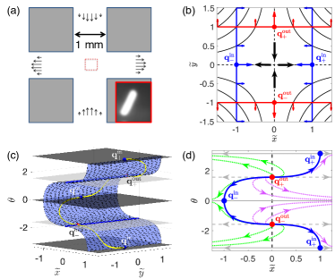
Figure 1: (a) Cross-flow experiment; data is obtained in the red square. Inset: 100X image of a fluorescent B. subtilis. (b) SFPs and SwIM edges (in red/blue) of the hyperbolic flow; $\alpha>0$. Arrows indicate the direction of $\hat{{\bf n}}$ (and the blocking direction) for the equilibria and the SwIM edges. Streamlines of the flow are plotted in black. (c) Stable SwIMs (blue surfaces) of the ${\bf q}^{\rm in}_{\pm}$ SFPs for $\alpha=1$. The black (gray) planes are stable (unstable) invariant surfaces. The yellow curves are heteroclinic orbits connecting pairs of SFPs. (d) Constant $y$ cross-section of the swimmer phase space. The blue orbits are cross-sections of the stable SwIMs.

In our model, an ellipsoidal swimmer in two dimensions (2D) is described by ${\bf q}=({\bf r},\hat{{\bf n}})$, comprising its position ${\bf r}=(x,y)$ and swimming direction $\hat{{\bf n}}=(\cos\theta,\sin\theta)$. Absent noise and active torques, a swimmer with a fixed swimming speed $v_{0}$ in a fluid velocity field ${\bf u}({\bf r})$ obeys Torney and Neufeld (2007); Khurana et al. (2011); Zöttl and Stark (2012); Arguedas-Leiva and Wilczek (2020)

$$\dot{{\bf r}}={\bf u}+v_{0}\hat{{\bf n}},\quad\quad\quad\dot{\theta}=\frac{\omega_{z}}{2}+\alpha\,\hat{{\bf n}}_{\perp}\cdot{\bf E}\hat{{\bf n}},$$ (1)

where $\omega_{z}=\hat{\bf z}\cdot(\nabla\times{\bf u})$ is the vorticity, $\hat{{\bf n}}_{\perp}=(-\sin\theta,\cos\theta)$, and ${\bf E}=(\nabla{\bf u}+\nabla{\bf u}^{\rm T})/2$ is the symmetric rate-of-strain tensor. The shape parameter $\alpha$ equals $(\gamma^{2}-1)/(\gamma^{2}+1)$, where $\gamma$ is the aspect ratio of the ellipse; $\alpha$ varies from $-1$ to $1$, where $\alpha=0$ is a circle, and $|\alpha|=1$ is a rod. Positive (negative) values of $\alpha$ correspond to swimming parallel (perpendicular) to the major axis. The case $\alpha=-1$ coincides with the dynamics of a propagating front element Mahoney et al. (2012) and the optimal (least-time) swimmer trajectories Rhoads et al. (2013); Gu et al. (2020).

Equation (1) with $v_{0}=0$ models passive transport. The linear hyperbolic flow, ${\bf u}=(Ax,-Ay)$ has a passive saddle fixed point at ${\bf r}={\bf 0}$. The $y$- and $x$-axes are the stable and unstable manifolds, respectively, defined as invariant sets whose points approach the passive fixed point forwards and backwards in time. Passive particles cannot cross these passive manifolds (Fig. 1b).

For swimmers in the hyperbolic flow, Eq. (1) becomes

$$\dot{\widetilde{x}}=\widetilde{x}+\cos\theta,\quad\dot{\widetilde{y}}=-\widetilde{y}+\sin\theta,\quad\dot{\theta}=-\alpha\sin(2\theta),$$ (2)

with dimensionless variables $\widetilde{{\bf r}}=(A/v_{0}){\bf r}$ and $\widetilde{t}=At$. The natural analogs of the passive fixed point are the fixed points of Eq. (2), called swimming fixed points (SFPs) Berman and Mitchell (2020). There are four SFPs. Two SFPs lie on the $y$-axis with the swimmer facing outward: ${\bf q}^{\rm out}_{\pm}=(\pm\hat{\bf y},\pm\hat{\bf y})$. The remaining SFPs lie on the $x$-axis with the swimmer facing inward: ${\bf q}^{\rm in}_{\pm}=(\pm\hat{\bf x},\mp\hat{\bf x})$. The SFPs are plotted in Fig. 1b-d. These equilibria are saddles, for all $v_{0}$ and $\alpha$.

We set $\alpha=1$, approximating the shape of B. subtilis as a rod. Since the SFPs are saddles, they possess stable and unstable manifolds in the $\widetilde{x}\widetilde{y}\theta$ phase space, which we call swimming invariant manifolds (SwIMs) to distinguish them from those for passive advection. For $\alpha>0$, the inward SFPs have two stable and one unstable direction. Hence, they each possess a 2D stable SwIM (Fig. 1c) which together form a warped sheet in phase space, referred to simply as the SwIM. The SwIM separates phase space into two regions: to the left [right] of the SwIM, all swimmer trajectories are ultimately leftward-escaping (LE) [rightward-escaping (RE)] (Fig. 1d).

The SwIM is only a strict phase-space barrier for perfectly smooth-swimming tracers, which is not the case for real swimmers. For example, tumbling bacteria apply brief active torques to suddenly change their swimming direction; we expect these bacteria to be able to cross the SwIM during their tumbles. Even for “smooth-swimming” bacteria, the swimming direction fluctuates; bacteria wiggle as they swim due to rotational diffusion Locsei and Pedley (2009); Junot et al. (2019) and the kinematics of swimming with helical flagella Hyon et al. (2012). Hence, bacteria near the SwIM may occasionally cross it due to these small fluctuations in $\theta$.

The SwIM seen in Fig. 1c produces one-way barriers to swimmers when projected into the $\widetilde{x}\widetilde{y}$ plane, barriers that are valid even for noisy swimmers. For a general 2D flow ${\bf u}({\bf r})$, a static, parametrized curve ${\bf R}(s)$ with local normal vector $\hat{{\bf N}}(s)$ is a one-way barrier to swimmers when the swimmer velocity across the curve, $[{\bf u}({\bf R}(s))+v_{0}\hat{{\bf n}}]\cdot\hat{{\bf N}}(s)$, is non-positive for all $\hat{{\bf n}}$. Hence, if the condition

$$-\frac{{\bf u}({\bf R}(s))\cdot\hat{{\bf N}}(s)}{v_{0}}\geq 1,\,\,\text{for all }s,$$ (3)

is met, then the curve ${\bf R}(s)$ is a one-way barrier with local blocking direction $\hat{{\bf N}}(s)$. For the hyperbolic flow, all non-stationary trajectories along the line $\widetilde{x}=-1$ move leftward, regardless of $\theta$ (Fig. 1d). Evaluating the left-hand side of Eq. (3) along this line [in dimensional variables, ${\bf R}(s)=(-v_{0}/A,s)$ and $\hat{{\bf N}}=\hat{\bf x}$], we obtain identically $1$. Therefore, this line is a one-way barrier, preventing rightward motion but not leftward. Furthermore, because Eq. (3) is independent of $\alpha$ and the time-dependence of $\hat{{\bf n}}$, we expect any curve satisfying it to be a one-way barrier for all swimmers, regardless of their shape or motility pattern. In particular, we expect the line $\widetilde{x}=-1$ to be a barrier to both the smooth-swimming and tumbling strains of bacteria.

Geometrically, Figs. 1c and 1d show that the line $\widetilde{x}=-1$ is the leftmost extent of the 2D SwIM projected into the $\widetilde{x}\widetilde{y}$ plane, i.e. it is the left edge of the SwIM. By symmetry, the right SwIM edge $\widetilde{x}=1$ is also a one-way barrier, which allows swimmers to pass through it from left to right, but not vice-versa. Hence, the stable SwIM edges form barriers to inward-swimming particles. Similarly, the horizontal edges of the 2D unstable SwIMs of the outward SFPs form one-way barriers, blocking outward-swimming particles (Fig. 1b).

We test our theoretical predictions with microfluidic experiments on swimming bacteria. We fabricate polydimethylsiloxane (PDMS) cells with channels of width and depth $1\,\,\,{\rm mm}$ in a cross-shaped geometry (Fig. 1a). Dilute bacteria suspensions are pumped into both ends of the vertical channel and out both ends of the horizontal channel using syringe pumps. Microscopy movies are recorded in the center of the channel at 40X. Passive tracer analysis reveals that the flow in the center (red square in Fig. 1a) is well-approximated by a 2D linear hyperbolic flow. The bacteria used are B. subtilis, either a smooth-swimming strain OI4139 or a green-fluorescent-protein-expressing (GFP) run-and-tumble strain 1A1266. The bacteria’s swimming speeds $v_{0}$ in the flow have a mean of $25\leavevmode\nobreak\ {\rm\mu m/s}$ and $16\leavevmode\nobreak\ {\rm\mu m/s}$ and standard deviation $11\leavevmode\nobreak\ {\rm\mu m/s}$ and $6\leavevmode\nobreak\ {\rm\mu m/s}$ for the smooth-swimming and tumbling GFP strains, respectively.

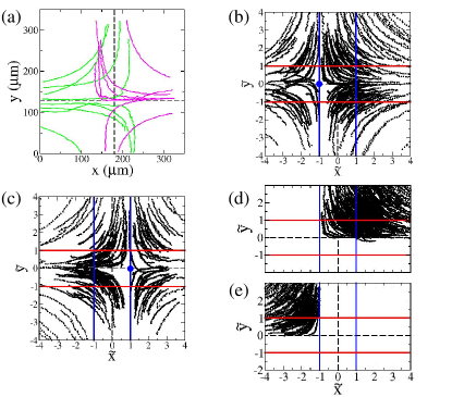
Figure 2: (a) Experimental trajectories for smooth-swimming B. subtilis; $A=0.44\,\,{\rm s}^{-1}$. Passive manifolds are shown with dashed lines. (b) Right-swimming trajectories. Positions are scaled by $v_{0}/A$. The theoretically predicted SFP ${\bf q}_{-}^{\rm in}$ (blue dot) and the SwIM edges (red and blue lines) are shown. (c) Left-swimming trajectories and ${\bf q}_{+}^{\rm in}$. (d) Rectified plot showing all trajectories as if leaving through the upper-right quadrant. (e) All trajectories entering with $|\widetilde{x}|>1$ rectified to enter the upper-left quadrant.

Figure 2 shows trajectories of smooth-swimming bacteria, some of which overlap (Fig. 2a). Trajectories of passive, non-swimming bacteria in the same experiment (Supplemental Material Fig. S1 SM ) are blocked by the vertical passive separatrix (dashed line in Fig. 2a). Hence, the region in Fig. 2a where the LE and RE swimmer trajectories overlap is a signature of the self-propulsion of the swimmers. Our theory predicts that the width of this region is the distance between the vertical SwIM edges shown in Fig. 1b, i.e. $2v_{0}/A$. In the experiments, $v_{0}$ is approximately constant in time for individual bacteria; however, different bacteria have different values for $v_{0}$ Kearns and Losick (2005). Consequently, the width of the overlap region is undetermined in Fig. 2a.

Variations in $v_{0}$ are accounted for by rescaling the spatial coordinates by $v_{0}/A$, as in Eq. (2). The scaled, non-dimensional trajectories are shown in Figs. 2b–e. The location of the inward SFPs and their SwIM edges is revealed by plotting trajectories for right-swimming and left-swimming bacteria separately (Figs. 2b and 2c). The behavior of inward-swimming bacteria near an inward SFP is similar to a passive tracer moving near the hyperbolic fixed point. The key difference is that active tracers moving near SFPs can cross the SwIM edge from $\left|\widetilde{x}\right|<1$ to $\left|\widetilde{x}\right|>1$, but not in the other direction.

The experimental data are consistent with the theoretically predicted one-way barrier property of the SwIM edges. This is clearest when we use the symmetry of Eqs. (2) [$(\widetilde{y},\theta)\mapsto(-\widetilde{y},-\theta)$ and $(\widetilde{x},\theta)\mapsto(-\widetilde{x},\pi-\theta)$] to rectify the trajectories, such that all trajectories are displayed as though entering from the upper inlet and escaping to the right. Under this transformation, Fig. 2d shows that all trajectories are bounded from the left by the SwIM edge at $\widetilde{x}=-1$, in agreement with the theory. Indeed, any bacterium crossing this SwIM edge from left to right would violate the one-way barrier property. Furthermore, all bacteria that enter with $\left|\widetilde{x}\right|>1$ (Fig. 2e, rectified such that initial $\widetilde{x}<-1$) are swept away from the center of the cell, consistent with the SwIM edges at $\left|\widetilde{x}\right|=1$ as barriers to inward-swimming bacteria.

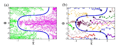
Figure 3: Experimental $\widetilde{x}\theta$ trajectories for smooth-swimming B. subtilis; $A=0.44\,\,\,{\rm s}^{-1}$. The theoretical SwIM ($\alpha=1$) is plotted in blue. (a) All trajectories. Leftward-escaping trajectories are green, and rightward-escaping trajectories are magenta. (b) Selected trajectories; the beginning of each is marked with an open square.

The delineation between LE and RE swimmers by the SwIM in the $\widetilde{x}\theta$ plane is shown experimentally in Fig. 3 (see SM for the measurement of $\theta$). Most of the trajectories in Fig. 3a respect this barrier, although there is a slight breach of the SwIM for some of the bacteria, due to the variations in $\theta$ discussed previously. These vertical fluctuations in individual trajectories (Fig. 3b) cause momentary crossings of the “horizontal” part of the SwIM.

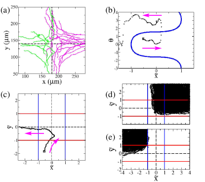
Figure 4: (a) Selected trajectories of run-and-tumble B. subtilis; $A=0.44\,\,{\rm s}^{-1}$. Passive manifolds are shown with dashed lines. (b) $\widetilde{x}\theta$ plot and (c) $\widetilde{x}\widetilde{y}$ trajectory for a single bacterium with well-defined tumbling events. (d) and (e) Scaled and rectified trajectories for tumbling bacteria, as in Figs. 2d and 2e.

Angular fluctuations are, of course, particularly pronounced for the tumbling strain of bacteria (Fig. 4a), leading to highly irregular $\widetilde{x}\theta$ trajectories. However, for bacteria with well-defined tumble events, the $\widetilde{x}\theta$ trajectories (Fig. 4b) give insight into the short-term direction (right or left) of their $\widetilde{x}\widetilde{y}$ motion (Fig. 4c). The bacterium in these two plots begins to the right of the SwIM; the corresponding $\widetilde{x}\widetilde{y}$ trajectory moves to the right during this period. The bacterium undergoes a significant tumble at $\widetilde{x}=0.2$, jumping above and to the left of the SwIM (Fig. 4b), with a corresponding change in direction in the $\widetilde{x}\widetilde{y}$ plane (Fig. 4c).

Despite the dramatic fluctuations in their orientations, the tumbling bacteria’s $\widetilde{x}\widetilde{y}$ trajectories respect the vertical lines $\widetilde{x}=\pm 1$ as one-way barriers, as predicted. Any RE swimmer must have entered with $\widetilde{x}>-1$ (Fig. 4d), and any swimmer that enters with $\widetilde{x}<-1$ must move leftward, away from the SwIM edge (Fig. 4e). Furthermore, though the trajectories in Fig. 4d cross the horizontal passive manifold, they do not cross the lower red line at $\widetilde{y}=-1$, respecting its outward-blocking nature.

In arbitrary flows, SwIM edges may not act as barriers for tumbling bacteria because they do not satisfy Eq. (3) in general. However, BIMs—which were introduced as one-way barriers to front propagation—always satisfy Eq. (3). In 2D time-independent flows, BIMs are the one-dimensional SwIMs for the $\alpha=-1$ case of Eq. (1) (i.e. $\alpha=-1$ trajectories ${\bf q}(t)$ that are asymptotic to SFPs), which satisfy the condition $-{\bf u}({\bf r}(t))\cdot\hat{{\bf n}}(t)/v_{0}=1$ Mitchell and Mahoney (2012); Mahoney et al. (2015); SM . Therefore, we now recognize BIMs as one-way barriers for all swimmers of a fixed swimming speed $v_{0}$, including those exhibiting rotational diffusion, tumbling, or other reorientation mechanisms. The robust bounding behavior occurs in our experiments because the SwIM edges coincide with the BIMs for linear hyperbolic flows. In general nonlinear flows, SwIM edges and BIMs depart from each other. Thus, the SwIM edges are the more relevant barriers for perfect smooth swimmers, whereas the BIMs are more relevant for noisy swimmers, as we illustrate with the following example.

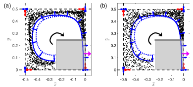
Figure 5: Bounding properties of SwIM edges and BIMs in a vortex flow; $v_{0}/U=0.1$, $\alpha=1$. (a) Initial positions (black dots) of smooth-swimmers that enter the grey square from the upper side and exit it on the right side (magenta arrow). The stable SwIM edge and stable BIM of the lower-right SFP are shown as solid blue and dotted blue curves, respectively. (b) Same as panel (a) for swimmers with rotational diffusivity $D_{r}$; $D_{r}L/U=0.86$.

We consider the swimmer dynamics Eq. (1) in the vortex-lattice flow Torney and Neufeld (2007); Khurana et al. (2011); Ariel et al. (2017); Berman and Mitchell (2020) ${\bf u}=(\sin(2\pi\widetilde{x})\cos(2\pi\widetilde{y}),-\cos(2\pi\widetilde{x})\sin(2\pi\widetilde{y}))$, where we use non-dimensional coordinates $\widetilde{{\bf r}}={\bf r}/L$ and $\widetilde{t}=tU/L$ for a flow with maximum speed $U$ and length scale $L$. Near ${\bf r}=0$, the flow is approximately the linear hyperbolic flow, with $A=2\pi$. Thus, the origin is surrounded by SFPs (Fig. 5a) analogous to those of Eq. (2) Berman and Mitchell (2020).

In analogy with the preceding microfluidic experiments that identified the positions of RE trajectories, we perform the following numerical experiment. We integrate the initial conditions of swimmers selected at random inside a single vortex cell but outside the grey square shown in Fig. 5a. We then plot only those initial positions for which the swimmer trajectory enters the grey square at the upper edge $\widetilde{y}=0.25$ and subsequently exits through the right edge at $\widetilde{x}=0$ (see SM for animations). These trajectories are analogous to the RE trajectories in the experimental hyperbolic flow. Figure 5a shows the result of the calculation for perfect smooth swimmers, along with the SwIM edge for the 2D stable SwIM of the vortex flow (solid curve) and the corresponding BIM (dotted curve). Clearly, these initial conditions are bounded by the SwIM edge, showing that the SwIM edge again bounds those trajectories that exit right, even in a nonlinear flow. We repeat the calculation with a moderate-intensity white noise term added to $\dot{\theta}$ in Eq. (1) to simulate rotational diffusion for realistic smooth-swimming bacteria Locsei and Pedley (2009). The resulting set of initial conditions (Fig. 5b) breaches the SwIM edge, but it remains bounded by the BIM, consistent with the absolute one-way barrier property of BIMs for all swimmers, regardless of their reorientation mechanism.

In summary, we have shown theoretically and experimentally that the trajectories of self-propelled particles in externally-driven fluid flows are constrained by the presence of one-way barriers, i.e. SwIM edges and BIMs. Despite the simplicity of our model, we are able to fully explain certain properties of the trajectories of swimming bacteria in an externally-driven microfluidic flow. Our SwIM framework provides a foundation for understanding the critical barrier structures that dominate the mixing of a wide range of self-propelled tracers in laminar flows. For example, BIMs must also block gyrotactic Guasto et al. (2012); Cencini et al. (2019) and chemotactic swimmers, since these barriers are independent of biases on the swimming direction. We further expect that the SwIM approach can be generalized to more complicated, time-periodic, time-aperiodic and weakly turbulent flows. It remains an open question how our approach may apply to the trajectories of self-propelled agents in active matter systems featuring self-driven flows, such as individual bacteria within a swarm Ariel et al. (2015) or motile defects in active nematics Sanchez et al. (2012); Shankar et al. (2018); Tan et al. (2019).