Solving two-parameter eigenvalue problems using an alternating method

Abstract

We present a new approach to compute selected eigenvalues and eigenvectors of the two-parameter eigenvalue problem. Our method requires computing generalized eigenvalue problems of the same size as the matrices of the initial two-parameter eigenvalue problem. The method is applicable for right definite problems, possibly after performing an affine transformation. This includes a class of Helmholtz equations when separation of variables is applied. We provide a convergence proof for extremal eigenvalues and empirical evidence along with a local convergence proof for other eigenvalues.

Keywords: Two-parameter eigenvalue problem, Alternating optimization, Helmholtz equation

AMS subject classifications: 65F15, 15A18, 15A69

1 Introduction

In this work we consider the two-parameter eigenvalue problem

$$(A_{1}+\lambda B_{1}+\mu C_{1})u =0,$$ (1)

$$(A_{2}+\lambda B_{2}+\mu C_{2})v =0$$

with matrices $A_{1},B_{1},C_{1}\in\mathbb{R}^{n\times n}$ and $A_{2},B_{2},C_{2}\in\mathbb{R}^{m\times m}$. A solution to this problem is given by possibly complex $(\lambda,\mu,u,v)$ if they fulfill (1) and $u,v\neq 0$. We call the pair $(\lambda,\mu)$ an eigenvalue of the two-parameter eigenvalue problem if $u,v\neq 0$ exist such that $(\lambda,\mu,u,v)$ satisfies (1) and we call the tensor product $u\otimes v$ an eigenvector of the two parameter eigenvalue problem (in the literature the pair $(u,v)$ is often referred to as the eigenvector; the terminology here is simply for convenience).

Two-parameter eigenvalue problems have been extensively studied [1, 23] and naturally arise in mathematical physics when separation of variables is applied. Consider for example the Helmholtz equation

$$\Delta u+\lambda u =0\quad\text{in }\Omega,$$

$$u =0\quad\text{on }\partial\Omega$$

where $\Omega=\{(x,y)\in\mathbb{R}^{2}:\left(\frac{x}{a}\right)^{2}+\left(\frac{y}{b}\right)^{2}<1,y>0\}$ is half of an open ellipse. Using elliptical coordinates, the problem can be reformulated into

$$\begin{aligned} v^{\prime\prime}(r)+(\lambda c^{2}\sinh^{2}(r)+\mu)v(r)&=0,\quad v(0)=0=v(R)\\ w^{\prime\prime}(\varphi)+(\lambda c^{2}\sin^{2}(\varphi)-\mu)w(\varphi)&=0,\quad w(0)=0=w(\pi)\end{aligned}$$ (2)

with $u(c\cosh(r)\cos(\varphi),c\sinh(r)\sin(\varphi))=v(r)w(\varphi)$ and $\mu\in\mathbb{R}$ (this will be explained in Section 3). This is of the form (1) after discretization. There are also many other applications that lead to (1), including delay differential equations [13] and optimization [22].

There are several numerical methods for solving this problem. The traditional approach [1] solves an $n^{2}\times n^{2}$ generalized eigenvalue problem (4) to find all solutions. Another possibility is Jacobi-Davidson type methods discussed in [9, 7]. These methods work well in finding eigenvalues close to a given target value. In [16] a Sylvester-Arnoldi type method is described that can be used to find a small subset of eigenvalues and uses that Sylvester equations can be solved efficiently. Another possibility is based on homotopy continutation, for example discussed in [18, 5]. These aim to find all eigenvalues.

We present a new algorithm that can be seen as an alternating method as they are for example considered in [10] for tensors. A similar approach is used in [2] and [24]. In these methods they alternatingly solve the first eigenvalue problems for $\lambda$ while fixing $\mu$ and the second eigenvalue problem for $\mu$ while fixing $\lambda$, and repeating the process. Another similar approach was taken in [20]. In there it is described how to transform a two-parameter eigenvalue problem with $n\gg m$ into a nonlinear eigenvalue problem and using techniques for nonlinear eigenvalue problems. By contrast, our method will choose either $\lambda$ or $\mu$ and solve two coupled linear eigenvalue problems alternatingly. This aims to reduce the complexity of finding one solution to (1). The complexity is the one of solving a generalized eigenvalue problem with matrices of size $n\times n$. Hence, the number of operations is $o(n^{3})$ for one solution. While we only establish global convergence for extremal eigenpairs, empirically our algorithm also finds all solutions, with $o(n^{5})$ cost. It will turn out that this method can find eigenvalues based on their index. The index of an eigenvalue of multiparameter eigenvalue problems is a generalisation of ordering real eigenvalues of a standard symmetric eigenvalue problems [23, Ch. 1]. We will need the following assumptions to hold:

1. All matrices are symmetric;

2. The matrices $C_{2}$ and $C_{1}\otimes B_{2}-B_{1}\otimes C_{2}$ are positve definite and $C_{1}$ is negative definite.

Notice that in example (2) the second derivative is indeed a symmetric operator, and $\sinh^{2}(r)>0$ and $\sin^{2}(\varphi)>0$ almost everywhere. A discrete version of these equations hence leads to a problem of the type (1) that satisfies the assumptions A.1 and A.2 up to signs.

Remark 1.

We only require the matrices $C_{1}$, $C_{2}$, and $C_{1}\otimes B_{2}-B_{1}\otimes C_{2}$ to be definite, however we chose these specific definiteness assumptions for convenience as to not have a list of all cases in the following theorems.

Remark 2.

The assumptions are not restrictive for right definite two parameter eigenvalue problems, that is for two parameter problems with positive or negative definite $C_{1}\otimes B_{2}-B_{1}\otimes C_{2}$. Indeed we can always find an affine transformation of (1) satisfying the definiteness assumptions.

First we can always find an affine transformation to make one matrix definite. Assume $C_{2}$ is indefinite. We can then perform the affine transformation

$$B_{1} \leftarrow B_{1}-\frac{v^{\top}B_{2}v}{v^{\top}C_{2}v}C_{1}$$

$$B_{2} \leftarrow B_{2}-\frac{v^{\top}B_{2}v}{v^{\top}C_{2}v}C_{2}$$

with $v$ such that $v^{\top}C_{2}v>0$. The new $B_{1}$ is negative definite, as the positive definiteness of $C_{1}\otimes B_{2}-B_{1}\otimes C_{2}$ implies that

$$(u^{\top}C_{1}u)(v^{\top}B_{2}v)-(u^{\top}B_{1}u)(v^{\top}C_{2}v)>0$$

for any $u$ and $v$. If $C_{2}$ is definite we can do the following in a similar fashion, and if $C_{2}$ is semidefinite but not definite, then $C_{1}$ is definite. We may therefore assume $B_{1}$ to be negative definite. Now let $u=\operatorname*{arg\,min}\frac{u^{\top}C_{1}u}{u^{\top}B_{1}u}$ be a minimizer. We can perform the affine transformation

$$C_{1} \leftarrow C_{1}-(\frac{u^{\top}C_{1}u}{u^{\top}B_{1}u}-\epsilon)B_{1}$$

$$C_{2} \leftarrow C_{2}-(\frac{u^{\top}C_{1}u}{u^{\top}B_{1}u}-\epsilon)B_{2}$$

for a sufficiently small $\epsilon>0$. Now the positive definiteness of $C_{1}\otimes B_{2}-B_{1}\otimes C_{2}$ and negative definiteness of $B_{1}$ implies that the new $C_{2}$ is positive definite and negative definiteness of $B_{1}$ and minimality of $u$ implies negative definiteness of the new $C_{1}$.

Note that when replacing $B_{1},B_{2}$ and $C_{1},C_{2}$ by the linear combination of matrices

$$\tilde{B}_{1}=b_{1}B_{1}+b_{2}C_{1},\quad\tilde{B}_{2}=b_{1}B_{2}+b_{2}C_{2}$$

and

$$\tilde{C}_{1}=c_{1}B_{1}+c_{2}C_{1},\quad\tilde{C}_{2}=c_{1}B_{2}+c_{2}C_{2}$$

and find the eigenvalue $(\tilde{\lambda},\tilde{\mu})$, we can recover the original eigenvalue $(\lambda,\mu)$ via

$$\lambda=b_{1}\tilde{\lambda}+c_{1}\tilde{\mu},\quad\mu=b_{2}\tilde{\lambda}+c_{2}\tilde{\mu}.$$

This article is organized as follows: In Section 2, we first motivate our method and state useful results from multiparameter eigenvalue theory. Afterwards we discuss fixed point properties of the algorithm and prove convergence for extremal eigenvalues. Finally, we examine the time complexity of our method briefly. In Section 3, we show that a class of boundary value problems satisfies our assumptions if properly discretized. Finally, we exhibit results of numerical experiments in Section 4.

2 An alternating algorithm for the two-parameter problem

In this section, we derive our algorithm and prove local convergence for all eigenvalues and global convergence for extremal eigenvalues. First, let us fix our notation. By $\otimes$ we denote the tensor product. For vectors this can be seen as the outer product, i.e., $u\otimes v$ corresponds to the rank-one matrix $uv^{\top}$. The tensor product of matrices then corresponds to a linear operator acting on matrices, i.e., the product $A\otimes B$ acts on the matrix $X$ by $AXB^{\top}$. This means that $(A\otimes B)(u\otimes v)=(Au\otimes Bv)$. It can also be seen as the Kronecker product for matrices [6, Ch. 12]. Then the product of two vectors $u\otimes v$ can be reshaped into a rank-one matrix.

2.1 Derivation of the algorithm

The two-parameter eigenvalue problem (1) can be reduced to two generalized eigenvalue problems [1]. For this define the operators acting on $n\times m$ matrices

$$\begin{aligned} M_{0}=B_{1}\otimes C_{2}-C_{1}\otimes B_{2},\\ M_{1}=A_{1}\otimes C_{2}-C_{1}\otimes A_{2},\\ M_{2}=B_{1}\otimes A_{2}-A_{1}\otimes B_{2}.\end{aligned}$$ (3)

A straightforward computation shows that a solution of (1) satisfies

$$\begin{aligned} M_{1}(u\otimes v)+\lambda M_{0}(u\otimes v)=0,\\ M_{2}(u\otimes v)+\mu M_{0}(u\otimes v)=0.\end{aligned}$$

Hence, solutions of (1) are also rank-one solutions $X$ of the system of generalized matrix eigenvalue problems

$$\begin{aligned} M_{1}(X)+\lambda M_{0}(X)=0,\\ M_{2}(X)+\mu M_{0}(X)=0,\end{aligned}$$ (4)

which are of size $nm\times nm$. Note that the eigenvectors are shared between the two generalized eigenvalue problems. Also under our assumptions solutions of (4) lead to solutions of (1). This is a well known consequence of classical theory [1, 23]. We provide a self contained proof for completeness.

Lemma 3.

Under the assumptions A.1 and A.2, the eigenvectors of the generalized eigenvalue problem $M_{1}(X)+\lambda M_{0}(X)=0$ are either rank one or are a linear combination of rank-one eigenvectors. A rank-one eigenvector is then also an eigenvector of the corresponding two-parameter eigenvalue problem.

Proof.

The assumption A.2 ensures that the eigenspaces of each subproblem in (4) is spanned by rank-one matrices. To see this, first note that the operator $M_{0}$ is negative definite, and $M_{1}$ and $M_{2}$ are symmetric. Therefore all eigenvalues of $\eqref{matrixev}$ are real. Second, we can without loss of generality assume $-C_{1}$ and $C_{2}$ to be identity matrices, else we just transform the matrices to $\tilde{A_{1}}=(-C_{1})^{-\frac{1}{2}}A_{1}(-C_{1})^{-\frac{1}{2}}$, $\tilde{B_{1}}=(-C_{1})^{-\frac{1}{2}}B_{1}(-C_{1})^{-\frac{1}{2}}$, etc., and $\tilde{u}=(-C_{1})^{\frac{1}{2}}u$, $\tilde{v}=C_{2}^{\frac{1}{2}}v$. Then $M_{0}$ and $M_{1}$ are operators in the form of a Sylvester equation, i.e., they have the form

$$M_{0}=B_{1}\otimes I_{m}+I_{n}\otimes B_{2},$$

$$M_{1}=A_{1}\otimes I_{m}+I_{n}\otimes A_{2}.$$

A solution to (4) then satisfies

$$\left((A_{1}+\lambda B_{1})\otimes I_{m}+I_{n}\otimes(A_{2}+\lambda B_{2})\right)(X)=0,$$

i.e., $X$ is a zero solution of a Sylvester equation. Such operators possess an orthonormal basis of rank-one eigenvectors, namely $u\otimes v$, where $u$ is an eigenvector of $(A_{1}+\lambda B_{1})$ and $v$ of $(A_{2}+\lambda B_{2})$ [11, Theorem 4.4.5], both of which are real symmetric and therefore possess an orthonormal basis of eigenvectors. It follows that $X$ is a sum of rank-one eigenvectors corresponding to the eigenvalue $0$. The dimension equals that of the null space of $M_{1}(X)+\lambda M_{0}(X)$, i.e., the geometric multiplicity of $\lambda$.

We next show that a rank-one solution to just one of the eigenvalue problems in (4) suffices to get a solution of the initial problem (1). Indeed, assume that $X=u\otimes v$ solves the second eigenvalue problem in (4). We then get

$$0= M_{1}(u\otimes v)+\lambda M_{0}(u\otimes v)$$

$$= A_{1}u\otimes C_{2}v-C_{1}u\otimes A_{2}v+\lambda B_{1}u\otimes C_{2}v-\mu C_{1}u\otimes B_{2}v$$

$$= (A_{1}+\lambda B_{1})u\otimes C_{2}v-C_{1}u\otimes(A_{2}+\lambda B_{2})v,$$

which holds true if and only if there is a $\mu$ such that

$$-\mu C_{1}u =(A_{1}+\lambda B_{1})u,$$

$$-\mu C_{2}v =(A_{2}+\lambda B_{2})v.$$

This implies (1). ∎

We can conclude that (1) has essentially $nm$ solutions which can be obtained by computing the rank-one solutions of one of the eigenvalue problems in (4). In the following, we select the first of these eigenvalue problems.

The assumptions imply that the operators $M_{0}$ and $M_{1}$ are symmetric and $M_{0}$ is negative definite. Thus, the solution of

$$M_{1}(X)+\lambda M_{0}(X)=0$$ (5)

with maximal eigenvalue $\lambda$ can be obtained by maximizing the Rayleigh quotient

$$\mathfrak{R}(X)=\frac{\langle X,M_{1}(X)\rangle}{\langle X,-M_{0}(X)\rangle},$$ (6)

and since the solution is a rank-one matrix, we can just maximize $\mathfrak{R}(u\otimes v)$ over $u$ and $v$. For convenience, define the functions

$$a_{1}(u) =u^{\top}A_{1}u, \quad b_{1}(u) =u^{\top}B_{1}u, \quad c_{1}(u) =u^{\top}C_{1}u,$$

$$a_{2}(v) =v^{\top}A_{2}v, \quad b_{2}(v) =v^{\top}B_{2}v, \quad c_{2}(v) =v^{\top}C_{2}v.$$

The assumption A.2 assures that $b_{2}(v)C_{1}-c_{2}(v)B_{1}$ and $c_{1}(u)B_{2}-b_{1}(u)C_{2}$ are positive definite. We can then write

$$\mathfrak{R}(u\otimes v)=-\frac{u^{\top}(c_{2}(v)A_{1}-a_{2}(v)C_{1})u}{u^{\top}(c_{2}(v)B_{1}-b_{2}(v)C_{1})u}.$$

For fixed $v$ the matrix in the denominator is negative definite. Hence, the maximal value is given by the maximal eigenvalue of the generalized eigenvalue problem

$$\left(c_{2}(v)A_{1}-a_{2}(v)C_{1}\right)u=\lambda(b_{2}(v)C_{1}-c_{2}(v)B_{1})u,$$ (7)

and respectively fixing $u$, the maximal value of

$$\mathfrak{R}(u\otimes v)=-\frac{v^{\top}(a_{1}(u)C_{2}-c_{1}(u)A_{2})v}{v^{\top}(b_{1}(u)C_{2}-c_{1}(u)B_{2})v}$$

is given by the maximal eigenvalue of

$$\left(a_{1}(u)C_{2}-c_{1}(u)A_{2}\right)v=\lambda(c_{1}(u)B_{2}-b_{1}(u)C_{2})v.$$ (8)

These are generalized eigenvalue problems with matrices of size $n\times n$ and $m\times m$, while (5) is a generalized eigenvalue problem of size $nm\times nm$.

A similar alternating procedure is of course obtained when minimizing the Rayleigh quotient in (6), i.e., when aiming at the smallest eigenvalue of (5). More generally, nothing even prevents us from updating $u$ and $v$ with non-extremal eigenpairs of the subproblems (7) and (8) in the hope of finding non-extremal eigenpairs of (5). For instance, we can solve (7) for the $i$-th eigenvalue and (8) for the $j$-th eigenvalue, for some fixed $i$ and $j$. This idea motivates Algorithm 1.

We will call a pair of eigenvectors $u$ and $v$ a fixed point of Algorithm 1 if it simultaneously solves the eigenvalue problems (7) and (8). Then choosing the corresponding index $(i,j)$ the algorithm will not change $u$ and $v$ anymore, provided eigenvalues are simple.

1

Input : Matrices $A_{i},B_{i},C_{i}$ for $i=1,2$ satisfying A.1 and A.2 and index $(i,j)$.

Output : Eigenvalue $(\lambda,\mu)$ of index $(i,j)$ with corresponding eigenvector $u\otimes v$.

2 select random nonzero $u_{0}\in\mathbb{R}^{n}$;

3 for k=1,2,3,… do

4       $a_{1}:=a_{1}(u_{k-1}),\quad b_{1}:=b_{1}(u_{k-1}),\quad c_{1}:=c_{1}(u_{k-1})$;

5       compute the eigenvector $v_{k}$ corresponding to the $j$-th smallest eigenvalue of the symmetric right definite generalized eigenvalue problem

$$\left(a_{1}C_{2}-c_{1}A_{2}\right)v=\lambda(c_{1}B_{2}-b_{1}C_{2})v;$$

6       $a_{2}:=a_{2}(v_{k});\quad b_{2}:=b_{2}(v_{k});\quad c_{2}:=c_{2}(v_{k})$;

7       compute the eigenpair $(u_{k},\lambda_{k})$ corresponding to the $i$-th smallest eigenvalue of the symmetric right definite generalized eigenvalue problem

$$\left(c_{2}A_{1}-a_{2}C_{1}\right)u=\lambda(b_{2}C_{1}-c_{2}B_{1})u;$$

8      

9 end for

10$\lambda:=\lambda_{k}$,  $u:=u_{k}$, $v:=v_{k}$, $\mu:=-\frac{a_{2}+\lambda b_{2}}{c_{2}}$;

11

return $(\lambda,\mu)$ and $u\otimes v$.

Algorithm 1 Alternating Algorithm for solving two-parameter eigenvalue problems.

2.2 Fixed point properties

Our aim in this section is to show that in principle we can find all rank-one eigenpairs of the problem (5), and hence of (1), by finding fixed points of the subproblems (7) and (8) solved in Algortihm 1 for all possible input indices $(i,j)\in\{1,\dots,n\}\times\{1,\dots,m\}$. The first step in this direction is the following lemma, which shows that a fixed point of the algorithm indeed provides a solution to (5) and (1).

Lemma 4.

Let $u$ and $v$ simultaneously solve (7) and (8). Under the assumptions A.1 and A.2 both eigenvalues coincide. Moreover, setting $\mu:=-\frac{a_{2}(v)+\lambda b_{2}(v)}{c_{2}(v)}$, $(u\otimes v,\lambda)$ is an eigenpair of (5) and $(u,v,\lambda,\mu)$ is a solution for the two-parameter problem (1).

Proof.

Denote the eigenvalue in (7) and (8) by $\hat{\lambda}$ and $\tilde{\lambda}$, respectively. Then multiplying (7) by $u^{\top}$ and (8) by $v^{\top}$, we get

$$c_{2}(v)a_{1}(u)-a_{2}(v)c_{1}(u)=-\hat{\lambda}(c_{2}(v)b_{1}(u)-b_{2}(v)c_{1}(u))$$

and

$$c_{2}(v)a_{1}(u)-a_{2}(v)c_{1}(u)=-\tilde{\lambda}(c_{2}(v)b_{1}(u)-b_{2}(v)c_{1}(u)).$$

Since A.2 implies $c_{2}(v)b_{1}(u)-b_{2}(v)c_{1}(u)<0$, we have $\hat{\lambda}=\tilde{\lambda}=:\lambda$. Collecting terms in (7) and (8) gives

$$c_{2}(v)A_{1}u+c_{2}\lambda B_{1}u-(a_{2}+\lambda b_{2}(v))C_{1}u =0,$$

$$-c_{1}(u)A_{2}v-c_{1}\lambda B_{2}v+(a_{1}+\lambda b_{1}(u))C_{2}v =0.$$

Dividing the first equation by $c_{2}(v)>0$ and the second by $-c_{1}(u)>0$, we get (1) with $\mu=-\frac{a_{1}(u)+\lambda b_{1}(u)}{c_{1}(u)}$, if

$$\frac{a_{2}(v)+\lambda b_{2}(v)}{c_{2}(v)}=\frac{a_{1}(u)+\lambda b_{1}(u)}{c_{1}(u)}.$$

This equation is however just a consequence of

$$c_{2}(v)a_{1}(u)-a_{2}(v)c_{1}(u)=-\lambda(c_{2}(v)b_{1}(u)-b_{2}(v)c_{1}(u)).$$

By the considerations in Section 2.1 $(u\otimes v,\lambda)$ is also a solution of (5). ∎

The previous lemma does not yet let us conclude that all solutions of (1) occur as fixed points of Algorithm 1 when varying the input index $(i,j)$. To show this, we need to introduce the notion of the index of an eigenvalue $(\lambda,\mu)$ of the two-parameter eigenvalue problem.

Definition 5.

An eigenvalue $(\lambda,\mu)$ of the two-parameter eigenvalue problem has the index $(i,j)$ if $0$ is the $i$-th smallest eigenvalue of $A_{1}+\lambda B_{1}+\mu C_{1}$ and the $j$-th smallest eigenvalue of $A_{2}+\lambda B_{2}+\mu C_{2}$.

If $0$ is a multiple eigenvalue of $A_{1}+\lambda B_{1}+\mu C_{1}$ or $A_{2}+\lambda B_{2}+\mu C_{2}$, then the corresponding eigenvalue of the two-parameter eigenvalue problem has multiple indices as well. Under the assumption A.1 every real valued eigenvalue of the two-parameter eigenvalue problem has an index since the matrices $A_{1}+\lambda B_{1}+\mu C_{1}$ and $A_{2}+\lambda B_{2}+\mu C_{2}$ are symmetric. More important for us is the following result, which immediately follows from [23, Theorem 1.4.1].

Theorem 6.

Under the assumptions A.1 and A.2 there is a unique eigenvalue $(\lambda,\mu)$ to every index $(i,j)\in\{1,\dots,n\}\times\{1,\dots,m\}$.

The idea is now to show that the index in the sense of Definition 5 of the eigenvalue solution provided by a fixed point of Algorithm 1 coincides with the given input index $(i,j)$. Together with Theorem 6 this then implies that all solutions can be obtained this way. For this we need the following version of Sylvester’s law of inertia.

Lemma 7.

Let $A,B$ be symmetric matrices and $I+B$ be positive definite. Then $\lambda_{i}$ is the $i$-th largest eigenvalue of $A$ if and only if it is the $i$-th largest eigenvalue of the generalized eigenvalue problem

$$(A+\lambda_{i}B)u=\lambda(I+B)u.$$

Proof.

Consider the matrices $M_{1}=A-\lambda_{i}I$ and $M_{2}=(I+B)^{-\frac{1}{2}}(A-\lambda_{i}I)(I+B)^{-\frac{1}{2}}$. The matrix $M_{2}$ is well defined since $I+B$ is positive definite and since $(I+B)^{-\frac{1}{2}}=((I+B)^{-\frac{1}{2}})^{T})$ is invertible, $M_{1}$ and $M_{2}$ are congruent and therefore have the same number of positive and respectively negative eigenvalues by Sylvester’s law of inertia [12, Theorem 4.5.8].

We can rewrite $M_{2}$ in the following way:

$$M_{2} =(I+B)^{-\frac{1}{2}}(A-\lambda_{i}I)(I+B)^{-\frac{1}{2}}$$

$$=(I+B)^{-\frac{1}{2}}(A+\lambda_{i}B-\lambda_{i}B-\lambda_{i}I)(I+B)^{-\frac{1}{2}}$$

$$=(I+B)^{-\frac{1}{2}}(A+\lambda_{i}B)(I+B)^{-\frac{1}{2}}-\lambda_{i}I.$$

This implies that $A$ and $(I+B)^{-\frac{1}{2}}(A+\lambda_{i}B)(I+B)^{-\frac{1}{2}}$ have the same number of eigenvalues that are smaller or respectively larger than $\lambda_{i}$. Since the eigenvalues of $(I+B)^{-\frac{1}{2}}(A+\lambda_{i}B)(I+B)^{-\frac{1}{2}}$ are the same as the eigenvalues of the generalized eigenvalue problem

$$(A+\lambda_{i}B)u=\lambda(I+B)u$$

the claim is proven. ∎

We are now in a position to prove the main result.

Theorem 8.

Let $(i,j)$ be the input index of Algorithm 1 and let $(u,v,\lambda,\mu)$ be a fixed point of Algorithm 1. Then the output $(\lambda,\mu)$ is the eigenvalue of problem (1) with index $(i,j)$ in the sense of Defintion 5 and $u\otimes v$ is the corresponding eigenvector.

Proof.

Let $(u,v)$ be a fixed point of Algorithm 1 and let $(\lambda,\mu)$ be the corresponding eigenvalue, i.e., $\lambda$ is the $i$-th smallest eigenvalue of the generalized eigenvalue problem

$$\left(c_{2}(v)A_{1}-a_{2}(v)C_{1}\right)u=\lambda(b_{2}(v)C_{1}-c_{2}(v)B_{1})u.$$

The Assumption A.2 guarantees that $b_{2}(v)C_{1}-c_{2}(v)B_{1}$ is positive definite, we may therefore apply Lemma 7. It follows that $\lambda$ is the $i$-th smallest eigenvalue of the matrix

$$c_{2}(v)A_{1}-a_{2}(v)C_{1}-\lambda(b_{2}(v)C_{1}-c_{2}(v)B_{1})+\lambda I_{n}=c_{2}(v)(A_{1}+\lambda B_{1}+\mu C_{1})+\lambda I_{n},$$

where we substituted $a_{2}(v)=-\lambda b_{2}(v)-\mu c_{2}(v)$. This implies that $0$ is the $i$-th smallest eigenvalue of $A_{1}+\lambda B_{1}+\mu C_{1}$ since $c_{2}(v)>0$ is positive by Assumpotion A.2.

Similarly, $\lambda$ is the $j$-th smallest eigenvalue of the generalized eigenvalue problem

$$\left(a_{1}(u)C_{2}-c_{1}(u)A_{2}\right)v=\lambda(c_{1}(u)B_{2}-b_{1}(u)C_{2})v.$$

We can again use Lemma 7 to conclude that $\lambda$ is the $j$-th smallest eigenvalue of the matrix

$$a_{1}(u)C_{2}-c_{1}(u)A_{2}-\lambda(c_{1}(u)B_{2}-b_{1}(u)C_{2})+\lambda I_{m}=-c_{1}(u)(A_{2}+\lambda B_{2}+\mu C_{2})+\lambda I_{m},$$

where we substituted $a_{1}(u)=-\lambda b_{1}(u)-\mu c_{1}(u)$. Note that the values for $\mu$ coincide in a fixed point, as was shown in Lemma 4. The Assumption A.2 implies that $c_{1}(u)<0$ and therefore $0$ is the $j$-th smallest eigenvalue of $A_{2}+\lambda B_{2}+\mu C_{2}$. ∎

Remark 9.

This result made use of the definiteness of $C_{1}$ and $C_{2}$. If instead $B_{1}$ and $B_{2}$ are definite one obtains a similar correspondence of input indices and indices of the eigenvalue when considering an alternating method resulting from the eigenvalue problem $(M_{2}+\mu M_{0})(X)=0$ instead of $(M_{1}+\lambda M_{0})(X)=0$.

Theorem 8 implies that if Algorithm 1 converges, then it computes a solution to the two-parameter eigenvalue problem (1).

Corollary 10.

Let $(u_{k},v_{k},\lambda_{k})$ be a sequence generated by Algorithm 1. If $u_{k}$ and $v_{k}$ converge in the projective sense to $u$ and $v$, i.e., convergence is up to sign flip if we choose normalized $u_{k}$ and $v_{k}$ in each step, then $\lambda_{k}$ converge to $\lambda$ and $u,v,\lambda$ are fixed by Algorithm 1. Therefore the output $(\lambda,\mu)$ is the eigenvalue of problem (1) with index $(i,j)$ in the sense of Defintion 5 and $u\otimes v$ is the corresponding eigenvector.

Proof.

Let $X_{2k}=u_{k}\otimes v_{k}$ and $X_{2k+1}=u_{k+1}\otimes v_{k}$. Since $u_{k}$ and $v_{k}$ converge to $u$ and $v$ respectively $x_{k}$ converges to $u\otimes v$. Define $\hat{\lambda}_{k}=\mathfrak{R}(X_{2k+1})$. Notice that $\lambda_{k}=\mathfrak{R}(X_{2k})$ is the eigenvalue corresponding to (7) and $\hat{\lambda}_{k}$ is the eigenvalue corresponding to (8) . By continuity of the Rayleigh quotient $\mathfrak{R}$, we get $\lim_{k\to\infty}\lambda_{k}=\lim_{k\to\infty}\hat{\lambda}_{k}=\lambda$. By continuity of the functions $a_{1},b_{1},c_{1},a_{2},b_{2},c_{2}$ and continuity of eigenvalues of a nonsingular generalized eigenvalue problem, we get that $u$ and $v$ are eigenvectors of the eigenvalue problems (7) and (8) with eigenvalue $\lambda$ and continuity also ensures that the eigenvalue is still the $i$-th or respectively $j$-th largest. Hence, $(u,v,\lambda,\mu)$ satisfies the conditions of Theorem 8. ∎

2.3 Geometric interpretation and rate of convergence

Algorithm 1 can be interpreted geometrically. For a given input index $(i,j)$ we look for the intersection of the curves

$$\gamma_{i}=\{(\lambda,\mu):\text{ $0$ is the $i$-th largest eigenvalue of }A_{1}+\lambda B_{1}+\mu C_{1}\},$$

$$\zeta_{j}=\{(\lambda,\mu):\text{ $0$ is the $j$-th largest eigenvalue of }A_{2}+\lambda B_{2}+\mu C_{2}\}.$$

As a consequence of [14, Theorem II.6.1] and definiteness of $C_{1}$ and $C_{2}$, these curves are continuous and piecewise analytic, and the corresponding eigenvectors are also piecewise analytic. In a fashion similar to [3, Lemma 2.2] we can derive the tangent line of $\gamma_{i}$ and $\zeta_{j}$ at an analytic point $(\lambda,\mu)$ with the corresponding eigenvectors. We can choose $\lambda$ as a local variable and obtain

$$(A_{1}+\lambda B_{1}+\mu(\lambda)C_{1})u(\lambda)=0$$

which implies

$$(A_{1}+\lambda B_{1}+\mu(\lambda)C_{1})u^{\prime}(\lambda)=-(B_{1}+\mu^{\prime}(\lambda)C_{1})u(\lambda).$$

Multiplying both equations to with $u(\lambda)^{\top}$ on the left results in

$$a_{1}(u(\lambda))+\lambda b_{1}(u(\lambda))+\mu(\lambda)c_{1}(u(\lambda)) =0,$$

$$b_{1}(u(\lambda))+\mu^{\prime}(\lambda)c_{1}(u(\lambda) =0.$$ (9)

The tangent line $T_{\gamma}$ of $\gamma_{i}$ at a point $(\lambda_{0},\mu(\lambda_{0}))$ is therefore given by

$$T_{\gamma}=\{(\lambda,\mu):\mu{c_{1}(u(\lambda_{0}))}=-\big{(}{a_{1}(u(\lambda_{0}))+\lambda b_{1}(u(\lambda_{0}))\big{)}}\}$$

and similarly the tangent line $T_{\zeta}$ of $\zeta_{j}$ at a point $(\lambda_{0},\mu(\lambda_{0}))$ is given by

$$T_{\zeta}=\{(\lambda,\mu):\mu{c_{2}(v(\lambda_{0}))=-\big{(}{a_{2}(v(\lambda_{0}))+\lambda b_{2}(v(\lambda_{0}))\big{)}}}\},$$

where $v(\lambda_{0})$ is the corresponding eigenvector of $A_{2}+\lambda_{0}B_{2}+\mu(\lambda_{0})C_{2}$. Examining Algorithm 1, it can therefore be interpreted as follows:

1. Start at a point $(\lambda,\mu)$ of $\gamma_{i}$ and compute it’s tangent line $T_{\gamma}$;

2. compute the intersection point $(\lambda,\mu)$ of $T_{\gamma}$ and $\zeta_{j}$ and compute the tangent line $T_{\zeta}$;

3. compute the intersection point $(\lambda,\mu)$ of $T_{\zeta}$ and $\gamma_{i}$ and compute the tangent line $T_{\gamma}$;

4. go to step 2.

We can use this interpretation to estimate the local rate of convergence. Notably, this interpretation is related to Newton’s method for computing an intersection point of two functions $f$ and $g$. While Newton’s method would compute a new iterate via

$$f(x_{k})-g(x_{k})+(f^{\prime}(x_{k})-g^{\prime}(x_{k}))(x_{k+1}-x_{k})=0,$$

our method performs two steps via

$$f(x_{k})+f^{\prime}(x_{k})(x_{k+1}-x_{k})=g(x_{k+1})\quad\text{and}\quad g(x_{k+1})+g^{\prime}(x_{k+1})(x_{k+2}-x_{k+1})=f(x_{k+2}).$$ (10)

This allows us to prove local quadratic convergence in a similar fashion to a standard Newton’s method.

Proposition 11.

Let $f,g:U\subset\mathbb{R}\to\mathbb{R}$ be differentiable with Lipschitz continuous derivatives $f^{\prime}$ and $g^{\prime}$ and corresponding constants $\alpha$ and $\beta$. Furthermore, let $|f^{\prime}(x)-g^{\prime}(x)|\geq\gamma>0$ for all $x$. Then a sequence $x_{k}$ generated by (10) satisfies

$$|\Delta x_{k}|(1-\frac{\beta}{2}|\Delta x_{k}|) \leq\frac{\alpha}{2\gamma}|\Delta x_{k-1}|^{2},$$

$$|\Delta x_{k+1}|(1-\frac{\alpha}{2}|\Delta x_{k+1}|) \leq\frac{\beta}{2\gamma}|\Delta x_{k}|^{2},$$

where $\Delta x_{k}=x_{k+1}-x_{k}$.

Proof.

We start with (10) and with a Taylor expansion for $g$ we get

$$f(x_{k})+f^{\prime}(x_{k})\Delta x_{k}=g(x_{k+1})=g(x_{k})+g^{\prime}(x_{k})\Delta x_{k}+\int_{0}^{1}\big{(}g^{\prime}(x_{k}+s\Delta x_{k})-g^{\prime}(x_{k})\big{)}\Delta x_{k}ds.$$

A Taylor expansion of $f$ and $g(x_{k})=f(x_{k-1})+f^{\prime}(x_{k-1})\Delta x_{k-1}$ leads to

$$f(x_{k})=g(x_{k})+\int_{0}^{1}\big{(}f^{\prime}(x_{k-1}+s\Delta x_{k-1})-f^{\prime}(x_{k-1})\big{)}\Delta x_{k-1}ds.$$

Combining both equations, we get

$$\big{(}f^{\prime}(x_{k})-g^{\prime}(x_{k})\big{)}\Delta x_{k}=\int_{0}^{1}\big{(}g^{\prime}(x_{k}+s\Delta x_{k})-g^{\prime}(x_{k})\big{)}\Delta x_{k}-\big{(}f^{\prime}(x_{k-1}+s\Delta x_{k-1})-f^{\prime}(x_{k-1})\big{)}\Delta x_{k-1}ds.$$

Using Lipschitz continuity and $|f^{\prime}(x)-g^{\prime}(x)|>\gamma$, we arrive at

$$\gamma|x_{k}|\leq\frac{\beta}{2}|x_{k}|^{2}+\frac{\alpha}{2}|x_{k-1}|^{2}.$$

The first inequality follows directly, and the second one can be derived analogously. ∎

We can apply this result, when the intersection point of $\gamma_{i}$ and $\zeta_{j}$ is an analytic point of both curves. Then we can describe both locally via smooth functions $\mu=f(\lambda)$ for $\gamma_{i}$ and $\mu=g(\lambda)$ for $\zeta_{j}$. The difference $|f^{\prime}-g^{\prime}|$ can be bounded with (9). We get $|f^{\prime}-g^{\prime}|\geq|\frac{b_{1}(u)}{c_{1}(u)}-\frac{b_{2}(v)}{c_{2}(v)}|>0$ by the definiteness assumption A.2.

2.4 Global convergence for extremal eigenpairs

So far, we have shown that if the algorithm converges, it returns the eigenvalue of the two-parameter eigenvalue problem with the desired index. For extremal indices, we can actually prove global convergence.

Theorem 12.

The sequences $u_{k}$ and $v_{k}$ generated by Algorithm 1 converge (up to normalization and sign flip) to a solution of (1) if the input index is either $(1,1)$ or $(n,m)$ and under the assumption that the respective eigenvalue is simple.

We use the following lemma for proving convergence when each step is at least as good as a line search.

Lemma 13.

Let $f:D\to\mathbb{R}$ be continuously differentiable, where $D\subset\mathbb{R}^{n}$ is open. Let $\{x_{k}\}_{k\in\mathbb{N}}\subset K\subset D$ and $g_{k}=\nabla f(x_{k})$ satisfy

$$f(x_{k+1})\leq f(x_{k}-\sigma g_{k})$$

for every $\sigma\in\mathbb{R}$ such that $x_{k}-\sigma g_{k}\in D$, where $K$ is compact. Then $g_{k}$ converges to zero as $k\to\infty$.

Proof of Lemma 13.

First note that $f(x_{k+1})\leq f(x_{k}-\sigma g_{k})$ for all $\sigma$ implies that $f(x_{k})$ is monotonically nonincreasing and $\{x_{k}\}_{k\in\mathbb{N}}\subset K$ implies that $f(x_{k})$ is bounded from below. Hence, $f(x_{k})$ converges to some value $\tilde{f}$ and since $x_{k}$ lies in a compact set, the gradients $g_{k}$ are bounded as well.

Now towards a contradiction assume that $\|g_{k}\|\geq 2\epsilon>0$ for some $\epsilon>0$ and every $k$. Else either $g_{k}$ converges to zero or we can choose a subsequence $g_{k^{\prime}}$ such that $\|g_{k^{\prime}}\|\geq 2\epsilon>0$. Since $g_{k}$ are bounded, there exists $\delta_{1}>0$ such that $x_{k}-\sigma g_{k}\in\tilde{K}\subset D$ for every $\sigma\in[0,\delta_{1}]$, where $\tilde{K}$ is also compact. Since $f$ is continuously differentiable, $\nabla f$ is uniformly continuous on $\tilde{K}$. Therefore, there is $\delta_{2}\in(0,\delta_{1}]$ such that

$$\|\nabla f(x_{k}-\xi g_{k})-g_{k}\|<\epsilon.$$

for all $\xi\in[0,\delta_{2}]$. By the mean value theorem, Cauchy-Schwarz inequality, and the assumption $\|g_{k}\|\geq 2\epsilon$, we have

$$f(x_{k})-f(x_{k}-\delta_{2}g_{k}) =\delta_{2}\nabla f(x_{k}-\xi g_{k})^{\top}g_{k}$$

$$\geq\delta_{2}\|g_{k}\|^{2}-\delta_{2}\|\nabla f(x_{k}-\xi g_{k})-g_{k}\|\|g_{k}\|$$

$$\geq\delta_{2}\|g_{k}\|^{2}-\delta_{2}\|g_{k}\|\epsilon$$

$$\geq\frac{\delta_{2}}{2}\|g_{k}\|^{2}\geq 2\delta_{2}\epsilon^{2}.$$

This yields the contradiction

$$\infty>f(x_{0})-\tilde{f}=\sum_{k=0}^{\infty}f(x_{k})-f(x_{k+1})\geq\sum_{k=0}^{\infty}f(x_{k})-f(x_{k}-\delta_{2}g_{k})\geq\sum_{k=0}^{\infty}2\delta_{2}\epsilon^{2}=\infty,$$

therefore $g_{k}$ converges to zero. ∎

Proof of Theorem 12.

Without loss of generality, assume that $C_{1}=-I_{n}$ and $C_{2}=I_{m}$. Finding the vectors $u$ and $v$ for the indices $(1,1)$ and $(n,m)$ corresponds to either minimizing or maximizing the Rayleigh quotient

$$\mathfrak{R}(X)=-\frac{\langle X,M_{1}(X)\rangle}{\langle X,M_{0}(X)\rangle}.$$

Its gradient is given by

$$\nabla\mathfrak{R}(X)=-\frac{2}{\langle X,M_{0}(X)\rangle}\left(M_{1}(X)+\mathfrak{R}(X)M_{0}(X)\right)$$

and if $X=u\otimes v$, then since $C_{1}=-I_{n}$ and $C_{2}=I_{m}$, we have

$$\nabla\mathfrak{R}(u\otimes v)=-\frac{2}{\langle u\otimes v,M_{0}(u\otimes v)\rangle}\left(u\otimes(A_{2}+\mathfrak{R}(u\otimes v)B_{2})v+(A_{1}+\mathfrak{R}(u\otimes v)B_{1})u\otimes v\right).$$

This shows that the gradient is an element in the tangent space of the rank-one matrix manifold at $u\otimes v$, which is given by

$$T_{u\otimes v}\mathcal{M}_{1}=\{x\otimes v+u\otimes y:x\in\mathbb{R}^{n},y\in\mathbb{R}^{m}\}.$$

Now assume every iterate of $u$ and $v$ are unit vectors. Then $-c_{1}(u)=1=c_{2}(v)$ and the Rayleigh quotient reads

$$\mathfrak{R}(u\otimes v)=\frac{a_{1}(u)+a_{2}(v)}{b_{1}(u)+b_{2}(v)}.$$

Now let $(\lambda,v)$ be an eigenpair of

$$\left(a_{1}(u)I_{m}+A_{2}\right)v=-\lambda(b_{1}(u)I_{m}+B_{2})v,$$

which is one step of Algorithm 1. It follows that $\lambda=\mathfrak{R}(u\otimes v)$ and

$$-\left(A_{2}+\lambda B_{2}\right)v=(a_{1}(u)+\lambda b_{1}(u))v.$$

The gradient is then

$$\nabla\mathfrak{R}(u\otimes v)=\frac{2}{\langle u\otimes v,M_{0}(u\otimes v)\rangle}\left(-u\otimes(a_{1}(u)+\lambda b_{1}(u))v+(A_{1}+\lambda B_{1})u\otimes v\right),$$

and is orthogonal to the subspace $\{u\otimes y:y\in\mathbb{R}^{m}\}\subset T_{u\otimes v}\mathcal{M}_{1}$ as

$$\langle\nabla\mathfrak{R}(u\otimes v),u\otimes y\rangle=\frac{2}{\langle u\otimes v,M_{0}(u\otimes v)\rangle}\left(-(a_{1}(u)+\lambda b_{1}(u))v^{\top}y+(a_{1}(u)+\lambda b_{1}(u))v^{\top}y\right)=0.$$

This was to be expected, as in each step we optimize the Rayleigh quotient with respect to the subspace $\{u\otimes y:y\in\mathbb{R}^{m}\}$ or respectively $\{x\otimes v:x\in\mathbb{R}^{n}\}$, which makes the gradient orthogonal to that respective space. This, together with $\nabla\mathfrak{R}(u\otimes v)\in T_{u\otimes v}\mathcal{M}_{1}$, implies that the gradient lies in $\{u\otimes y:y\in\mathbb{R}^{m}\}$ or respectively $\{x\otimes v:x\in\mathbb{R}^{n}\}$ after each half step.

We now only consider the case of minimizing the Rayleigh quotient, as maximizing can be done analogously. As we can choose our iterates $u_{k}$ and $v_{k}$ to be normalized, the iterates $X_{k}=u_{k}\otimes v_{k}$ lie in a compact set. As

$$v_{k+1}=\operatorname*{arg\,min}_{\|v\|=1}\mathfrak{R}(u_{k}\otimes v),$$

we have $\mathfrak{R}(X_{k+1})\leq\mathfrak{R}(X_{k}-\sigma\nabla\mathfrak{R}(X_{k}))$ since $X_{k}-\sigma\nabla\mathfrak{R}(X_{k})$ is of the form $u_{k}\otimes v$, and the $\mathfrak{R}$ is scaling invariant. We can thus use Lemma 13 and therefore $\nabla\mathfrak{R}(X^{k})$ converges to zero, implying that any convergent subsequence of $X_{k}$ converges to an eigenvector of $M_{1}(X)+\lambda M_{0}(X)=0$. Corollary 10 implies that this eigenvector corresponds to the eigenvalue of the correct index. Hence, since this eigenvalue is simple, the sequence $X_{k}$ only has one accumulation point up to sign flip. ∎

2.5 Complexity

We discuss time complexity of Algorithm 1. We assume $m=n$. Computing the eigendecomposition of a generalized eigenvalue problem needs $O(n^{\omega+\gamma})\subset o(n^{3})$ operations, where $\omega$ is the exponent of complexity of matrix multiplication and $\gamma>0$ [4]. This implies that the complexity for computing one eigenvalue of the two-parameter eigenvalue problem is $o(n^{3}k)$, where $k$ is the number of iterations in Algorithm 1 until a sufficient accuracy is achieved (empirically we observe $k=O(1)$). When computing all $n^{2}$ eigenvalues of the two-parameter eigenvalue problem, we therefore get a complexity of $o(n^{5}k)$ (and with $k=O(1)$ we get a complexity of $o(n^{5})$). However, a full eigenvalue decomposition is not always necessary. For extremal eigenvalues, we only need to compute the eigenvector corresponding to the largest or smallest eigenvalue, which is typically possible in $O(n^{2})$ operations, for example using Lanczos or LOBPCG [15]. Similarly, the $i$-th largest eigenvalue can often be computed in $O(n^{2}i)$ operations. In summary, computing an eigenvalue with index $(i,j)$ needs $O(n^{2}k\max(\min(i,n-i+1),\min(j,n-j+1))$ operations, where $k$ is the number of iterations necessary for the desired accuracy. If the matrices allow for fast matrix vector multiplication, for example if they are sparse with $O(n)$ nonzero entries, the complexity can be reduced further up to $O(nk\max(\min(i,n-i+1),\min(j,n-j+1))$ operations.

3 A class of PDE eigenvalue problems

We now present a class of PDE eigenvalue problems, which can be separated into an appropriate two-parameter eigenvalue problem. Let $\phi:(a,b)\times(c,d)\to U\subset\mathbb{R}^{2}$ be a diffeomorphism, with

$$g(x,y):=(D\phi(x,y))^{\top}D\phi(x,y)=\begin{pmatrix}g_{1}(x)+g_{2}(y)&0\\ 0&g_{1}(x)+g_{2}(y)\end{pmatrix},$$

and choose $g_{1},g_{2}>0$. This is always possible for such a function $g$ as $g(x,y)$ is positive definite and therefore $g_{1}(x)+g_{2}(y)>0$. Now let $\Omega=\phi((a,b)\times(c,d))$. We consider the Helmholtz equation

$$\Delta u+\lambda u=0\quad \text{on }\Omega,$$

$$u=0\quad \text{at }\partial\Omega.$$

We can now write $\Delta u$ in coordinates given by $\phi$. Then

$$(\Delta u)(\phi(x,y))= \frac{1}{\sqrt{\det(g(x,y))}}\nabla\cdot\left(\sqrt{\det(g(x,y))}g^{-1}(x,y)\nabla(u(\phi(x,y))\right)$$

$$= \frac{1}{g_{1}(x)+g_{2}(y)}\Delta(u(\phi(x,y))).$$

Making an ansatz $u(x,y)=v(x)w(y)$, we get

$$0 =v^{\prime\prime}(x)w(y)+v(x)w^{\prime\prime}(y)+\lambda g_{1}(x)v(x)w(y)+\lambda g_{2}(y)v(x)w(y)$$

$$=v(x)\big{(}w^{\prime\prime}(y)+\lambda g_{1}(x)w(y)-\mu w(y)\big{)}+w(y)\big{(}v^{\prime\prime}(x)+\lambda g_{2}(y)v(x)+\mu v(x)\big{)}.$$

Now let $v$ and $w$ satisfy

$$v^{\prime\prime}(x)+\lambda g_{1}(x)v(x)+\mu v(x) =0$$ (11)

$$w^{\prime\prime}(y)+\lambda g_{2}(y)w(y)-\mu w(y) =0,$$ (12)

and $0=v(a)=v(b)=w(c)=w(d)$. Then $u(x,y)=v(x)w(y)$ solves the original eigenvalue problem, and on a given discretrization (11) satisfies A.1 and A.2.

Example 14.

The complex function $\phi:\mathbb{C}\to\mathbb{C},z\mapsto z^{2}$. Then $D\phi(z)=2z$. Therefore with $z=x+iy$, we have

$$g(x,y)=\begin{pmatrix}2x&2y\\ -2y&2x\end{pmatrix}\begin{pmatrix}2x&-2y\\ 2y&2x\end{pmatrix}=\begin{pmatrix}4x^{2}+4y^{2}&0\\ 0&4x^{2}+4y^{2}\end{pmatrix}.$$

Example 15.

The complex function $\phi:\mathbb{C}\to\mathbb{C},z\mapsto e^{z}$. Then $D\phi(z)=e^{z}$. Therefore with $z=x+iy$, we have

$$g(x,y)=\begin{pmatrix}e^{x}\cos(y)&e^{x}\sin(y)\\ -e^{x}\sin(y)&e^{x}\cos(y)\end{pmatrix}\begin{pmatrix}e^{x}\cos(y)&-e^{x}\sin(y)\\ e^{x}\sin(y)&e^{x}\cos(y)\end{pmatrix}=\begin{pmatrix}e^{2x}&0\\ 0&e^{2x}\end{pmatrix}.$$

These coordinates describe an annulus.

Example 16.

The complex function $\phi:\mathbb{C}\to\mathbb{C},z\mapsto\cosh(z)$. Then $D\phi(z)=\sinh(z)$. Therefore with $z=x+iy$, we have

$$g(x,y)= \begin{pmatrix}\sinh(x)\cos(y)&\cosh(x)\sin(y)\\ -\cosh(x)\sin(y)&\sinh(x)\cos(y)\end{pmatrix}\begin{pmatrix}\sinh(x)\cos(y)&-\cosh(x)\sin(y)\\ \cosh(x)\sin(y)&\sinh(x)\cos(y)\end{pmatrix}$$

$$= \begin{pmatrix}\sinh^{2}(x)+\sin^{2}(y)&0\\ 0&\sinh^{2}(x)+\sin^{2}(y)\end{pmatrix}.$$

These are elliptical coordinates.

4 Numerical Experiments

(a)

(b)

Figure 1: Testing Algorithm 1 with input index $(1,1)$. Figure 1(a) depicts results for randomly generated $1000\times 1000$ matrices fulfilling Assumptions A.1 and A.2 and Figure 1(b) depicts results for a discretization of (2) on a $1000\times 1000$ grid.

(a) Two iterations

(b) Three iterations

(c) Four iterations

(d) Five iterations

(e) Six iterations

(f) Seven iterations

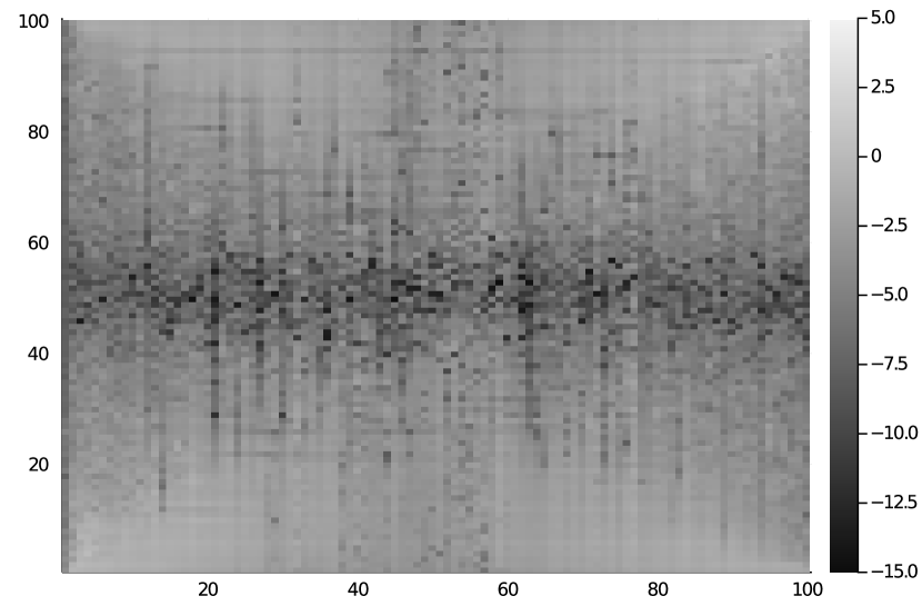
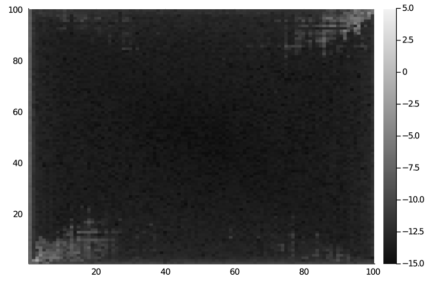
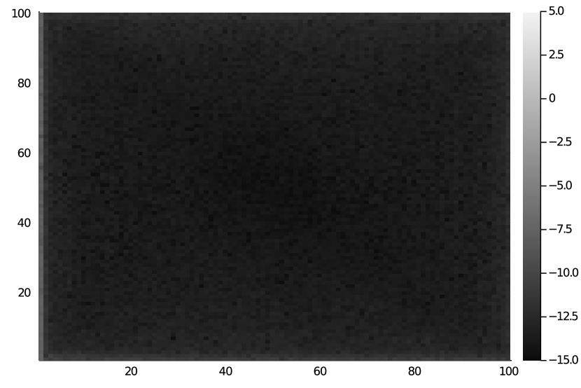
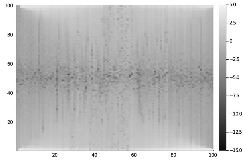
Figure 2: Testing Algorithm 1 with random $100\times 100$ matrices fulfilling the assumptions. Every picture is taken after solving one eigenvalue problem in line 4 or 6 of the algorithm. The axis label the indices of the computed eigenvalue and the colorscale shows the sum of the absolute values of the $i$-th and $j$-th eigenvalue in (1) on a logarithmic scale.

In this section, we present results from numerical experiments to test the performance of Algorithm 1. For a measure of the error we use Definition 5. For a given approximate eigenvalue $(\lambda,\mu)$ we compute the $i$-th smallest eigenvalue of $A_{1}+\lambda B_{1}+\mu C_{1}$ and the $j$-th smallest eigenvalue of $A_{2}+\lambda B_{2}+\mu C_{2}$ and take the sum of the respective absolute values. This quantity is zero if and only if $(\lambda,\mu)$ is an eigenvalue with index $(i,j)$. This is also the sum of the corresponding residual norms with the corresponding normalized eigenvectors.

In a first experiment we generated matrices satisfying Assumptions A.1 and A.2 randomly. For the matrices $A_{1}$ and $A_{2}$ we generated $n\times n$ and $m\times m$ matrices with independent standard Gaussian distributed entries and took the symmetric part. For the matrices $B_{1},B_{2},C_{1},C_{2}$ we generated matrices $S_{1}$ and $S_{2}$ with Gaussian distributed entries and an $n$ dimensional array $b_{1}$ with values uniformly distributed between $-0.5$ and $0.5$ and an $m$ dimensional array $b_{2}$ with values uniformly distributed between $-1.5$ and $-0.5$. We then chose the matrices

$$B_{1}=S_{1}\operatorname{Diag}(b_{1})S_{1}^{\top},\quad B_{2}=S_{2}\operatorname{Diag}(b_{2})S_{2}^{\top},\quad C_{1}=-S_{1}S_{1}^{\top},\quad C_{2}=S_{2}S_{2}^{\top},$$

where $\operatorname{Diag}(b_{i})$ is the matrix with the entries of $b_{i}$ on its diagonal.

(a) Two iterations

(b) Three iterations

(c) Four iterations

(d) Five iterations

(e) Six iterations

(f) Seven iterations

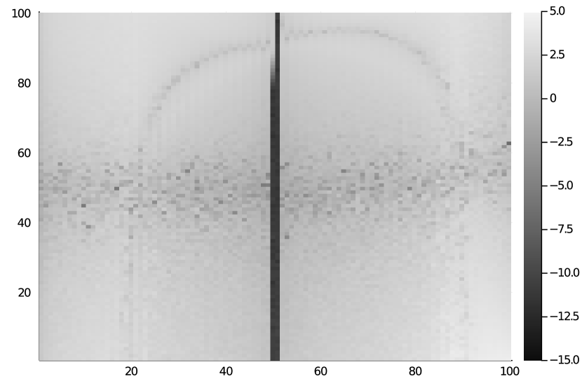
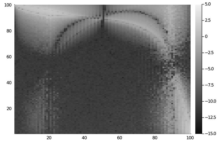
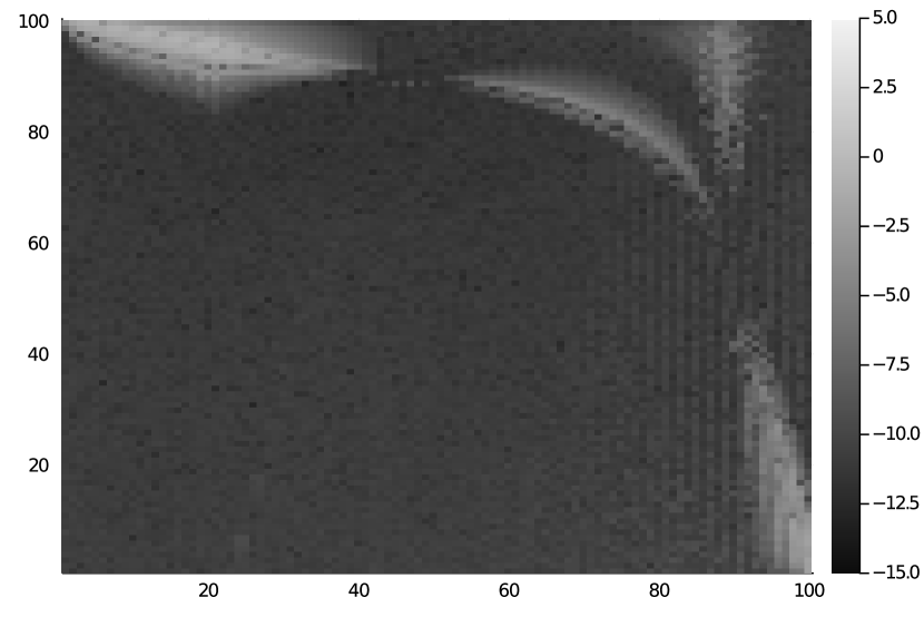
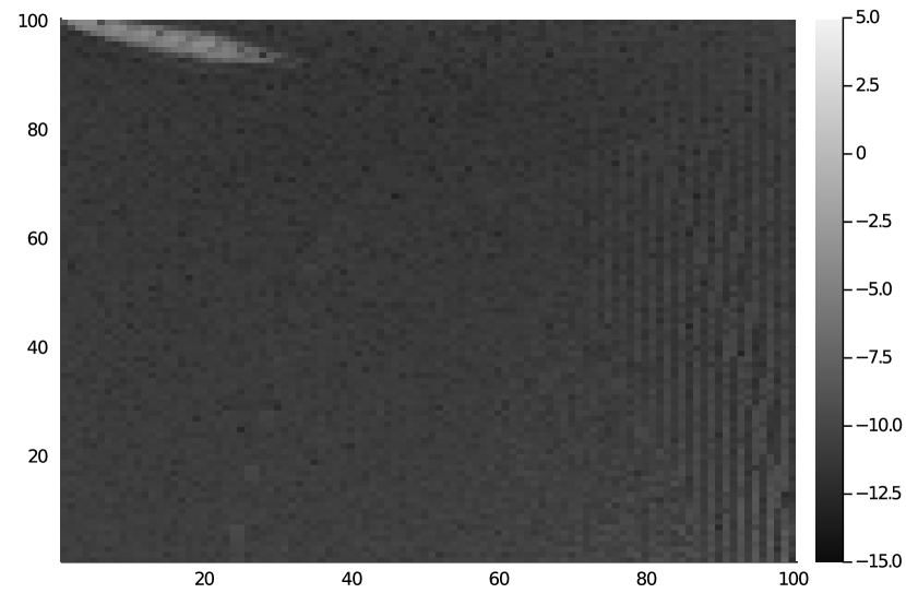
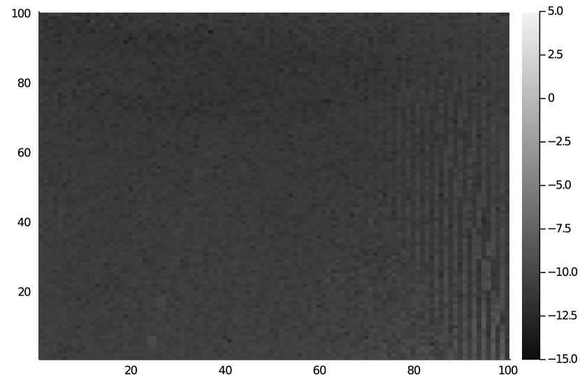
Figure 3: Testing Algorithm 1 with a discretization of (2) on a $100\times 100$ grid. Every picture is taken after solving one eigenvalue problem in line 4 or 6 of the algorithm. The axis label the indices of the computed eigenvalue and the colorscale shows the sum of the absolute values of the $i$-th and $j$-th eigenvalue in (1) on a logarithmic scale.

(a)

(b)

Figure 4: Comparing the computational time 4(a) and precision 4(b) for randomly generated examples with matrices of size $n\times n$ satisfying the assumption A.1 and A.2 for our method and twopareig from [19].

(a)

(b)

Figure 5: Comparing the computational time 5(a) and precision 5(b) for randomly generated examples with matrices of size $n\times n$ satisfying the assumption A.1 and A.2 for our method and twopareig from [19]. For this example the matrices $B_{1},B_{2},C_{1},C_{2}$ are diagonal matrices.

As a second example, we discretized the Helmholtz equation on half of an ellipse as in the example in Section 1, i.e.,

$$\begin{aligned} v^{\prime\prime}(r)+(\lambda c^{2}\sinh^{2}(r)+\mu)v(r)&=0,\quad v(0)=0=v(1)\\ w^{\prime\prime}(\varphi)+(\lambda c^{2}\sin^{2}(\varphi)-\mu)w(\varphi)&=0,\quad w(0)=0=w(\pi).\end{aligned}$$ (13)

For Figure 1, we generated $1000\times 1000$ matrices randomly in 1(a) and used a discretization on a $1000\times 1000$ grid in 1(b) as described above and used Algorithm 1 to find an eigenvalue with minimal $\lambda$, i.e., with input index $(1,1)$. After solving 6 and 7 eigenvalue problems respectively as described in lines 4 and 6 of Algorithm 1, we found an eigenvalue with an error of approximately $10^{-9}$ and $10^{-10}$ respectively, confirming the result of Theorem 12.

For Figure 2 we generated $100\times 100$ matrices satisfying Assumptions A.1 and A.2 as described above and use Algorithm 1 to find every eigenvalue, i.e., for every input index $(i,j)\in\{1,\dots,100\}\times\{1,\dots,100\}$. The axis describe the input index of Algorithm 1 and the greyscale describes the base ten logarithm of the error described above. An iteration is computing the solution of one eigenvalue problem in lines 4 and 6 of Algorithm 1. After 7 iterations the highest error was $4\cdot 10^{-8}$ and the smallest errors were in the range of machine precision.

In Figure 3 we used a discretization of the Helmholtz equation (13) on a $100\times 100$ grid and repeated the experiment of Figure 2 for the resulting matrices. Again, after 7 iterations the highest error was $3\cdot 10^{-8}$ and the smallest errors were in range of machine precision. These experiments suggest that Algorithm 1 can indeed be used to find every eigenvalue of right definite two-parameter eigenvalue problems.

In Figure 44(a) we compared the time of both Algorithm 1 and the algorithm twopareig[19] for computing every eigenvalue of a two-parameter eigenvalue problem of varying sizes $n=m$. We generated matrices satisfying the assumptions as above. Notice that Algorithm 1 can be run in parallel for different input indices to further improve efficiency. The experiment was run on a Intel Xeon Gold 6144 at 3.5 GHz with 384 GB RAM. We used 8 cores with 16 threads. We chose to solve 10 small eigenvalue problems in Algorithm 1, corresponding to $k=1,\dots,5$ in line 2. For larger $n$ our method was indeed faster, and the asymptotic slope of the time -$n$ graph on a loglog scale is smaller, indicating that the asymptotic computational cost is lower. In Figure 44(b) we measure the sum of the $n^{2}$ errors as described above. We observe that our method computed eigenvalues with higher accuracy.

Finally, we repeated the last experiment, but we chose $S_{1}=I_{n}=S_{2}$. This made the matrices $B_{1},B_{2},C_{1}$ and $C_{2}$ diagonal, which effectively transformed the generalized eigenvalue problems in Algorithm 1 into ordinary eigenvalue problems to further improve efficiency. When solving for every eigenvalue of the two-parameter problem, we can perform the left and right actions of $(-C_{1})^{-\frac{1}{2}}$ and $C_{2}^{-\frac{1}{2}}$ respectively and afterwards diagonalize $B_{1}$ and $B_{2}$. This justifies this experiment. The results are depicted in Figure 5. In Figure 55(a) we see that the alternating method is faster than the method twopareig[19] for even smaller $n$. Again our method is more accurate.

5 Conclusion and outlook

We presented a new method for computing eigenvalues of the two-parameter eigenvalue problem. Our approach only requires solving generalized eigenvalue problems of the size of the matrices of the two-parameter problem and can therefore reduce the complexity compared to conventional methods. Our method also uses a search for the eigenvalues by index, which makes it possible to find successive eigenvalues of the two-parameter eigenvalue problem without deflation.

So far the technique of our proof only established global convergence for extremal eigenvalues and under definiteness assumptions. The numerical experiments however indicated convergence for every eigenvalue. Proposition 11 gives insight into the local convergence, but a global convergence proof remains an open problem. Although there are many classes of two-parameter eigenvalue problems that satisfy the assumptions (eventually after performing an affine transformation), many other interesting applications do not. Therefore it would be important to investigate if a generalization to non-singular problems, i.e., the operator $M_{0}$ is invertible, as in [7] or even to the general case as in [8] is possible.

This paper relies heavily on the assumptions A.1 and A.2. A natural question is to relax these conditions, in particular the definiteness condition A.2. Indeed under weaker assumptions (such as when the matrices are almost definite, with a few eigenvalues of the opposite sign), using inertia laws [17] one can show that the generalized eigenvalue problem (4), and hence also (1), has many real eigenvalues. It would be of interest to investigate the applicability of the results here in such situations.

Finally, another interesting generalization that could be considered is to multiparameter eigenvalue problems with more than 2 parameters. The eigenvectors then form rank-one tensors similar to (4) [1]. Again an alternating approach as in [10] can be used, however our proof technique will not work and in practice the generalization will not easily assure convergence even for extremal indices. A similar approach using the Tensor-Train format is used in [21].

References

• [1] F. V. Atkinson. Multiparameter eigenvalue problems. Academic Press, New York-London, 1972. Volume I: Matrices and compact operators, Mathematics in Science and Engineering, Vol. 82.
• [2] Paul B. Bailey. The automatic solution of two-parameter Sturm-Liouville eigenvalue problems in ordinary differential equations. Appl. Math. Comput., 8(4):251–259, 1981.
• [3] Paul Binding and Patrick J. Browne. Two parameter eigenvalue problems for matrices. Linear Algebra Appl., 113:139–157, 1989.
• [4] James Demmel, Ioana Dumitriu, and Olga Holtz. Fast linear algebra is stable. Numer. Math., 108(1):59–91, 2007.
• [5] Bo Dong, Bo Yu, and Yan Yu. A homotopy method for finding all solutions of a multiparameter eigenvalue problem. SIAM J. Matrix Anal. Appl., 37(2):550–571, 2016.
• [6] Gene H. Golub and Charles F. Van Loan. Matrix Computations. The Johns Hopkins University Press, 4th edition, 2012.
• [7] Michiel E. Hochstenbach, Tomaž Košir, and Bor Plestenjak. A Jacobi-Davidson type method for the two-parameter eigenvalue problem. SIAM J. Matrix Anal. Appl., 26(2):477–497, 2004/05.
• [8] Michiel E. Hochstenbach, Christian Mehl, and Bor Plestenjak. Solving singular generalized eigenvalue problems by a rank-completing perturbation. SIAM J. Matrix Anal. Appl., 40(3):1022–1046, 2019.
• [9] Michiel E. Hochstenbach and Bor Plestenjak. A Jacobi-Davidson type method for a right definite two-parameter eigenvalue problem. SIAM J. Matrix Anal. Appl., 24(2):392–410, 2002.
• [10] Sebastian Holtz, Thorsten Rohwedder, and Reinhold Schneider. The alternating linear scheme for tensor optimization in the tensor train format. SIAM J. Sci. Comput., 34(2):A683–A713, 2012.
• [11] Roger A. Horn and Charles R. Johnson. Topics in matrix analysis. Cambridge University Press, Cambridge, 1994. Corrected reprint of the 1991 original.
• [12] Roger A. Horn and Charles R. Johnson. Matrix Analysis. Cambridge University Press, Cambridge, second edition, 2013.
• [13] Elias Jarlebring and Michiel E Hochstenbach. Polynomial two-parameter eigenvalue problems and matrix pencil methods for stability of delay-differential equations. Linear Algebra Appl., 431(3-4):369–380, 2009.
• [14] Tosio Kato. Perturbation theory for linear operators. Classics in Mathematics. Springer-Verlag, Berlin, 1995. Reprint of the 1980 edition.
• [15] A. V. Knyazev. Toward the optimal preconditioned eigensolver: Locally optimal block preconditioned conjugate gradient method. SIAM J. Sci. Comput., 23(2):517–541, 2001.
• [16] Karl Meerbergen and Bor Plestenjak. A Sylvester-Arnoldi type method for the generalized eigenvalue problem with two-by-two operator determinants. Numer. Linear Algebra Appl., 22(6):1131–1146, 2015.
• [17] Yuji Nakatsukasa and Vanni Noferini. Inertia laws and localization of real eigenvalues for generalized indefinite eigenvalue problems. Linear Algebra Appl., 578:272–296, 2019.
• [18] Bor Plestenjak. A continuation method for a weakly elliptic two-parameter eigenvalue problem. IMA J. Numer. Anal., 21(1):199–216, 2001.
• [19] Bor Plestenjak. Multipareig. https://www.mathworks.com/matlabcentral/fileexchange/47844-multipareig), MATLAB Central File Exchange. Retrieved January 29, 2021, 2021.
• [20] Emil Ringh and Elias Jarlebring. Nonlinearizing two-parameter eigenvalue problems. arXiv:1907.00913, 2019.
• [21] Koen Ruymbeek, Karl Meerbergen, and Wim Michiels. Subspace method for multiparameter-eigenvalue problems based on tensor-train representations. arXiv:2012.00815, 2020.
• [22] Shinsaku Sakaue, Yuji Nakatsukasa, Akiko Takeda, and Satoru Iwata. Solving generalized CDT problems via two-parameter eigenvalues. SIAM J. Optim., 26(3):1669–1694, 2016.
• [23] Hans Volkmer. Multiparameter eigenvalue problems and expansion theorems, volume 1356 of Lecture Notes in Mathematics. Springer-Verlag, Berlin, 1988.
• [24] Ji Xingzhi. An alternating variable iterative method for multiparameter eigenvalue problems. ca 1985.