A New Approach to Accent Recognition and Conversion for Mandarin Chinese

Abstract

Two new approaches to accent classification and conversion are presented and explored, respectively. The first topic is Chinese accent classification/recognition. The second topic is the use of encoder-decoder models for end-to-end Chinese accent conversion, where the classifier in the first topic is used for the training of the accent converter encoder-decoder model. Experiments using different features and model are performed for accent recognition. These features include MFCCs and spectrograms. The classifier models were TDNN and 1D-CNN. On the MAGICDATA dataset with 5 classes of accents, the TDNN classifier trained on MFCC features achieved a test accuracy of $54\%$ and a test F1 score of $0.54$ while the 1D-CNN classifier trained on spectrograms achieve a test accuracy of $62\%$ and a test F1 score of $0.62$. A prototype of an end-to-end accent converter model is also presented. The converter model comprises of an encoder and a decoder. The encoder model converts an accented input into an accent-neutral form. The decoder model converts an accent-neutral form to an accented form with the specified accent assigned by the input accent label. The converter prototype preserves the tone and foregoes the details in the output audio. An encoder-decoder structure demonstrates the potential of being an effective accent converter. A proposal for future improvements is also presented to address the issue of lost details in the decoder output.

Index Terms: Accent Recognition, Accent Conversion, Voice Conversion, MFCC, Spectrogram, encode-decode neural networks, speaker embeddings, x-vectors, speaker recognition, transfer learning

1 Introduction

Accent variation is one of the most critical issues of the state-of-the-art automatic speech recognition (ASR) systems, especially for Mandarin Chinese. As a language with many dialects, including Wu (spoken in Shanghai, Jiangsu and Zhejiang provinces) and Yue (spoken in Cantonese areas such as Hong Kong and Guangdong), Mandarin is spoken with significant variations, depending on speakers’ regional dwelling across the country. Therefore, it is very challenging for any ASR system trained on standard Mandarin to perform well while encountering speakers with varied accents across the country. Adapting a sophisticated Chinese accent classifier or recognition system could provide a strong improvement to the current ASR systems.

In addition, accent conversion can also be a great solution to improve ASR performance, in which a differently accented Chinese speech can be converted to a standard Chinese dialect. Moreover, accent conversion is of interest itself not only because it could possibly improve ASR performance, but because it may be advantageous in many other applications and use cases, such as second language learning.

Currently, much of the work done in the accent conversion domain is limited to pairwise training and conversion, which requires a model to be built between each pair of accents. This is a significant limitation, given that there are so many possible accents, and it is absolutely not feasible to train an additional model for each single pair of accents. Furthermore, most of the current work and research focus only on English, for example, different types of non-native English accents versus native American or British dialects.

In this work, we propose and compare two types of Chinese accent classifier models. One is a time delay neural network (TDNN) model trained through transfer learning. The other one is a one-dimensional (1D) convolutional neural network (CNN) model. We also present an end-to-end Chinese accent conversion model, which is built using an encoder-decoder model and one of our pre-trained accent classifiers.

The remainder of this paper is structured as follows. Section 2 reviews some previous work on accent conversion, voice conversion, and accent recognition. Section 3 introduces the detailed methodology of our accent classifier models and the accent converter model. Section 4 describes the experiments we conducted, in detail, and presents corresponding results. Finally, Section 5 summarizes the conclusions of this study, and discusses the potential work that we plan to carry out in the future.

2 Related Work

As mentioned, most of the work done on accent conversion is limited to pairwise training and conversion. Aryal et al. (2015) [1] train a deep neural network (DNN) articulatory synthesizer for a non-native speaker, then map the non-native articulatory space to a native speaker via Procrustes transformations, and drive the trained DNN. They evaluate their model through listening tests of intelligibility, voice identity, and non-native accentedness. Bearman et al. (2017) [2] present a neural network model that learns differences between a pair of accents and produces transformation between the pair of accents using the extracted MFCC features [3]. Their pairwise binary classifier achieves an accuracy of $98.2\%$ between American English and Indian accented English. Nonetheless, as they reveal in the paper, the reconstructed waveforms are guttural and noisy, because MFCC features may not always retain sufficient information for quality audio reconstruction. Zhao et al. (2019) [4] use an acoustic model trained on a native English speech corpus to extract speaker-independent phonetic posteriorgrams (PPGs), and train a speech synthesizer to map non-native speech PPGs into desired native spectral features, which are then reconstructed into high-quality waveforms.

A similar domain that has been studied a lot is speaker voice conversion. Mobin et al. (2016) [5] apply CNN to transform the voice of one speaker into another by manipulating not only the pitch, but also the timbre [3]. They also employ generative adversarial networks (GANs) to enhance their generative model’s performance. Mohammadi et al. (2014) [6] train a deep autoencoder to build representations of short-term spectra of multiple speakers, which enables voice conversion in a speaker-independent fashion.

As for accent detection, most work has been done on native and non-native English accents. Jiao et al. (2016) [7] propose a combination of long-term and short-term training to tackle both prosodic and articulation characteristics that differentiate accents. DNNs are used for long-term statistical features training, whereas recurrent neural networks (RNNs) are used for short-term acoustic features training. They managed to achieve a classification accuracy of $52.48\%$ over the $11$ accent classes. Sheng et al. (2017) build a CNN model to classify $3$ different non-native English accents, and achieve a classification test accuracy of $88.0\%$ over the $3$ accent classes. Hernandez et al. (2018) [8] train a neural network to classify speech accents in video games, and achieve a classification test accuracy of $71\%$ over $2$ accent classes.

Very little work has been done on Mandarin or other Chinese dialects. Zheng et al. (2005) [9] propose an approach to combine accent detection and accent adapted model selection for Chinese speech recognition. They build a Gaussian mixture model (GMM) accent classifier with MFCC features, and achieve an test accuracy of $86\%$ on the accented audio group. They then apply MAP/MLLR to enhance acoustic adaptation and model selection, and attain state-of-the-art acoustic modeling on Wu-accented Chinese speech, reducing the character error rate by an absolute amount of $1.0\%$ to $1.4\%$.

3 Methodology

This section presents the methodology for the two main topics presented here, namely, accent recognition and accent conversion.

3.1 Accent Recognition

Our proposed full accent converter model is composed of two parts: an accent recognition model component, and an accent conversion component. The accent conversion model training process is based on the accent recognition model. Therefore, an accent recognition model must be trained separately before training a complete end-to-end accent converter model. The end-to-end accent converter model structure is described in detail in Section 3.2. This section presents two different classifier model designs, using different speech feature sets, TDNN classifier on MFCC features, and 1D-CNN classifier on spectrogram features, respectively.

3.1.1 TDNN Classifier on MFCC

The first set of features are MFCCs, which have been widely used for decades and usually produces state-of-the-art results in speaker recognition [3], speech recognition, and many other related tasks in practice. Accent recognition is quite related to the speaker recognition problem, in the sense that accent is an important characteristic in distinguishing speakers. Since speaker recognition [3] is a more complex and better-studied area than accent recognition, it is reasonable to train a speaker recognition model first and perform transfer learning to do accent classification. Therefore, MFCC is selected for this experiment, as it is generally used in speaker recognition tasks.

x-vectors [10] provide robust neural network embeddings speaker recognition, and once combined with a customary Linear Discriminant Analysis (LDA) and Probabilistic Linear Discriminant Analysis (PLDA) [3], they achieve superior performance on various speaker recognition evaluation datasets. Therefore, training an x-vector model on Mandarin corpus is the first step of this process. Using the x-vectors as features for additional NN layers and a log softmax output layer, a transfer learning, we build a transfer learning process and train an accent classification model. The details of training process and model architecture is described in Section 4.2.1.

3.1.2 1D-CNN Classifier on Spectrogram

The second set of feature used, was the spectrogram. Spectrograms have demonstrate empirical effectiveness in accent detection and recognition [8]. As a visual representation of the spectrum of frequencies of signal for different time slices, spectrograms resemble an images with one dimension representing time. Therefore, image recognition techniques may be used directly on spectrograms. Convolutional Neural Networks (CNNs) have been successfully used to perform machine learning on images prolifically. Therefore, for the spectrogram features, we chose a CNN as classifier.

The spectrogram input for one audio file is in 2 dimensional format. Comparing this representation to images, it resembles gray-scale images for which there is only a single color channel, or the depth is 1 in the 3 dimensional representation. However, the semantics of the width dimension is very different from gray-scale images. The semantic of the width in spectrogram is time, which has a special nature of being presented in sequence along time. With this in mind, the CNN model chosen is 1D-CNN instead of 2D-CNN. While 2D-CNN is commonly used and has proven success for regular images, the semantic meaning of convolving spectrogram with 2D kernels which crosses both different frequencies and time at the same time of the convolution operation is unclear. In 2D images, the height and the width dimension could be considered to be the same concept or in the same domain, whereas in spectrogram it may not make sense to mix frequency and time in the same kernel. Due to the nature of having a time dimension, 1D-CNN is considered to be more suitable for machine learning on spectrogram data in our design. It is also important to note that Time Delay Neural Networks used in the previous section are also a type of one dimensional convolutional neural network. So, in nature, the two architectures are not very different. They just operate on different features (MFCC vs Spectral). The experimental implementation may be found in Section 4.2.2.

3.2 Accent Conversion

The accent converter model is an encoder-decoder model. The encoder takes, as input, features of the original audio and converts them to their accent-neutral representation, in the same feature space. The decoder then take the output of the encoder, which is the accent-neutral representation of the input in the input feature space, together with an accent label specifying the desired accent, and converts the encoded output into an accented features with the specified accent. The input to the encoder, the intermediate accent-neutral form (the output of the encoder), and the output of the decoder are all in the same feature space. Namely, the dimension of the encoder input, the encoder output, and the decoder output are identical. There are two inputs to the accent converter, which are the original audio’s features, and the desired accent label in one-hot format. There is one output from the accent converter, which is the accent-converted audio’s features. As an accent conversion system that takes in an audio file and outputs another audio file, preprocessing of extracting the features from the audio file and postprocessing of converting the features back to an audio file are necessary in addition to the converter model.

Different features could be used for the accent converter. One requirement for such features is that they should be able to be extracted from audio files (such as wav and mp3) and show also be usable in reproducing an output audio file. Ideally, the chosen features should help reduce the dimension/size of the data while preserving sufficient information for successful accent recognition and reconstruction of the audio file with an acceptable quality. In our first prototype,we use spectral features. Other features such as CELP [11] and combination of multiple features are also worth considering. CELP and other features related Linear Predictive Coding (LPC) [3] have been used for speech compression for decades and are prime candidates for usage in this manner. We will consider this in our future work (See Section 5.2.3).

The following two subsections describe the training process of the accent converter and the inference/test workflow of the accent converter, respectively.

3.2.1 Training

To train the converter to convert accented speech into accent-neutral speech, an accent classifier is introduced. An accent classifier which recognizes the accent class of speech is first trained using the features that will be used in the accent converter. The class labels are in one-hot format. After training the classifier, its weights will be fixed and it could be used to assess the accent score for each known accent in a speech in the feature space. Once the classifier is ready, it is used as part of a trainer model. The trainer is the encoder-decoder model with the intermediate output of the encoder connected to the fixed weight pre-trained classifier. The high-level structure of the trainer model is shown in Fig.1.

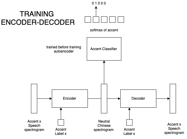
Figure 1: Converter training workflow

The trainer model has two inputs and two outputs.

• Input 1: encoder input – the original accented speech in the feature space

• Input 2: decoder input 2 – the desired output accent label in one-hot format

• Output 1: classifier output – the probability of the speech containing each accent as a vector

• Output 2: decoder output – converted accented speech in the feature space

The trainer model is composed of the encoder, the decoder, and the classifier. The connective relations among these modules are as follows:

• encoder output is connected to the classifier as the classifier input

• encoder output is connected to the decoder as the decoder input 1

The losses at both output branches, the classifier output and the decoder output, are back-propagated through the model. The two losses collectively guide the trainer model to learn. At the training time, trainer input 1 is the original speech feature, the trainer input 2 is the accent label of the original speech, the output 1 ground truth label used is a uniform probability distribution, as a vector, and the output 2 ground truth label is the original speech feature, identical to model input 1. As an example, the output 1 ground truth label for the MAGICDATA dataset (See Section 4.1.2), with 5 accent classes, would be $<0.2,0.2,0.2,0.2,0.2>$. Given this construction, with proper and sufficient training and in an ideal scenario, the output of the encoder should eventually produce accent-neutral speech in the feature space.

One potential drawback of this method is that there would never be training pairs whose input accent is different from the converted accent ground truth label. In the training the model is at best able to reconstruct the original input after performing conversion. This is a limit posted by the nature of the data, that it is not practical to have the same person speak multiple different accents.

At the converter training time, preprocessing and postprocessing for the conversion between input audio file and the speech features are already taken care of as a preparation step for the training. The trainer only deals with inputs and outputs in the feature space (spectrogram in our experiment). At inference time, preprocessing and postprocessing must be included to achieve an end-to-end conversion system, as described in 3.2.2.

3.2.2 Inference

After the training process is completed via the trainer, the encoder and decoder will ideally have proper weights for the accent conversion task. The accent converter model is the combination of the trained encoder and the trained decoder. The inference/test workflow of the accent converter is shown in Fig.2.

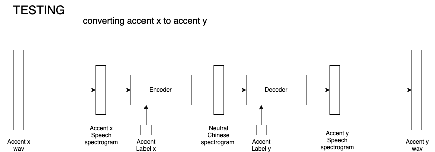
Figure 2: Converter inference workflow

As the encoder and the decoder are trained on features of the speech instead of the original audio file, preprocessing of feature extraction from the audio file and postprocessing for the purpose of reconstruction from feature to audio are necessary components for completing the system workflow, producing an end-to-end accent conversion.

The converter model has two inputs and one output.

• Input 1: encoder input – original accented speech in the feature space (after preprocessing)

• Input 2: decoder input 2 – desired output accent label in one-hot format

• Output: decoder output – converted accented speech in the feature space (before postprocessing)

The accent converter model is composed of the encoder and the decoder after they are trained using the trainer model. The connection relation between the encoder and the decoder is as follows:

• encoder output is connected to the decoder as decoder input 1

At the converter inference time, additional preprocessing and postprocessing for conversion between input audio and the speech features are added so that the system takes as input, an audio file (such as wav or mp3) and a desired accent label (one-hot format) and produces the accent-converted audio.

4 Experiments and Results

This section describes the datasets used in our experiments, the implementation details and results of the accent recognition models, and the implementation details and results of the accent conversion models.

4.1 Data

Two corpora used are Aishell-2 [12] and MAGICDATA [13]. Here, each dataset is described briefly.

4.1.1 Aishell-2 Corpus

The Aishell-2 [12] is a Chinese Mandarin speech corpus published by Beijing Shell Technology Co., Ltd. The contents and descriptions of the full corpus are as follows:

• $1000$ hours of speech data (around $1$ million utterances)

• includes segmented transcripts

• $1991$ speakers ($845$ male and $1146$ female)

• provides speaker demographic information including age, gender, and accent region (north or south)

• recorded in indoor environments using high fidelity microphone and downsampled to $16kHz$

• manual transcription accuracy is above $95\%$

Aishell-2 is by far the largest open-source Mandarin speech corpus and it was used to train a speaker recognition model, which was used as a pre-trained model to perform the transfer learning on accent recognition.

One drawback of Aishell-2 is that it labels accent region only in two categories of north and south. Since there are many accents across the country, dividing them purely by north and south is not desirable grouping for our purposes. For example, the Shanghai accent of Mandarin (Wu dialect spoken area) is quite different from the Guangdong accent Mandarin (where Cantonese is also spoken), but they are both labeled as one southern accent; whereas the Beijing accent (usually considered as standard Mandarin) is labeled as northern even though it shares much common with the Shanghai accent of Mandarin. Therefore, labeling accents by province is much more reasonable than simply tagging them northern or southern. This is where the MAGICDATA corpus comes into place, where it provides more fine-grained labels on accents, labeled by province.

4.1.2 MAGICDATA Corpus

The MAGICDATA Mandarin Chinese Read-Speech Corpus [13] is developed by MAGICDATA Technology Co., Ltd. The contents and descriptions of the corpus are presented here:

• $755$ hours of speech, mostly mobile recorded data

• includes segmented transcripts

• $1080$ speakers from different accent areas in China

• provides speaker demographic information including age, gender, and accent region (by province)

• sentence transcription accuracy higher than $98\%$

• recordings collected in quiet indoor environments

• speech data coding and speaker information file

• diversified domain of recording text, including interactive Q&A, music search, SNS messages, home command and control

• Training set, validation set, and test set in a ratio of $51:1:2$

As mentioned in Section 4.1.1, MAGICDATA provides fine-grained labels on speakers’ accents by a province label. The training set contains speakers from $28$ provinces, and the test set portrays speakers from $8$ provinces. The data distribution over the provinces is very unbalanced, as depicted in Fig.3. To balance the data distribution, we focused on a subset of provinces, and grouped them into $5$ classes by accent similarities and geographical proximity, as shown in table 1.

class label	provinces
chuan	si chuan $\cup$ chong qing
dongbei	ji lin $\cup$ liao ning $\cup$ hei long jiang
guan	bei jing $\cup$ tian jin $\cup$ he bei
wu	zhe jiang $\cup$ shang hai $\cup$ jiang su
yue	guang dong $\cup$ guang xi

Table 1: MAGICDATA classes

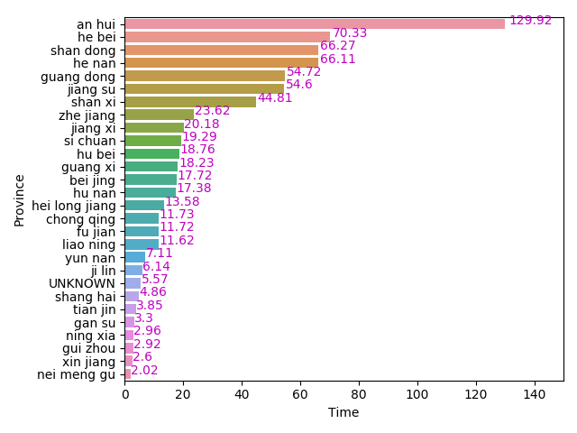
Figure 3: MAGICDATA training set data distribution, in terms of time (hours) versus province.

4.1.3 Feature Extraction

For the training, two audio features were used: MFCC and spectrogram.

For MFCC features, $30$ cepstral coefficients are extracted with a frame-length of $25ms$. Audios are sampled to $16kHz$. The resulting MFCC features is with dimension $30$ per frame. [3]

Spectrogram features were extracted by using the WORLD Vocoder [14], with a Fast Fourier transform transform (FFT) size of $256$, and a frame period of $10ms$. The choice of a relatively small FFT size was due to memory constraints. The audio was sampled at $16kHz$. The resulting spectrogram features produce a dimension of $(129,T)$, where $T$ is the audio length.

4.2 Accent Recognition

In this section two two accent classification models are introduced and used in our experiments.

4.2.1 TDNN on MFCC With Transfer Learning

As mentioned in Section 3.1.1, an x-vector speaker recognition embedding is trained following the same model structure as in [10]. We followed the Kaldi toolkit recipe for VoxCeleb-v2 (VoxCeleb2) provided at https://github.com/kaldi-asr/kaldi/tree/master/egs/voxceleb/v2. Aishell-2 data was used to train the x-vector model because it is by far the largest Mandarin speech corpus, containing $1991$ speakers with a balanced demographic distribution. Only $40\%$ of the full corpus was used to reduce the training time. Utterances were selected at random to prevent any unbalanced distribution. The details about the data split are shown in table 2.

$3$-fold data augmentation was used following the approach of [10], which randomly adds background speech (babble), music, and noise, and applies reverberation to the original recordings, and combines the original recordings, with two augmented copies. MFCC features were extracted as described in Section 4.1.3. The model training configuration and train/validation accuracies are presented in table 2.

LDA/PLDA [15] transformations with an output dimension of $200$ were also trained to transform the x-vectors from their original $512$ dimensions to lower dimensional space, more suitable for discriminating the speaker class labels. A trial file of $44784$ pairs of utterances was selected from the test set for scoring. The resulting EER and DCF results are listed in table 2. The model achieves an EER of $3.4\%$, which is in tune with the x-vector model trained on the VoxCeleb2 corpus [10].

Data Split	Training Configuration
Train set: $195944$ utterances	Number of epochs: $3$
Dev set: $27994$ utterances	Number of iterations: $80$
Test set: $55984$ utterances	Initial learning rate: $0.001$
Training Results	Momentum: $0.5$
Train accuracy: $98.3\%$	Loss: Cross-entropy
Validation accuracy: $97.9\%$	Metric: Accuracy
Trial file EER: $3.392\%$	-
minDCF($p=0.01$): $0.499$	-
minDCF($p=0.001$): $0.057$	-

Table 2: x-vector data split, training configuration and model results

At this point, we performed transfer learning using the pre-trained x-vector embedding. As mentioned in Section 4.1.2, MAGICDATA provides fine-grained labels on accent areas by province, which is more suitable than Aishell-2 for the accent classification task. Therefore, only MAGICDATA was used during the transfer learning process. The $5$ accent classes are chuan, dongbei, guan, wu, and yue, as described in Section 4.1.2. The number of utterances used for training and data split details are shown in table 3.

Data Split	Training Configuration
Train set: $100135$ utterances	Number of epochs: $10$
Test set: $25030$ utterances	Number of iterations: $135$
Training Results	Initial learning rate: $0.05$
Train accuracy: $80\%$	Momentum: $0.5$
Validation accuracy: $53\%$	Loss: Cross-entropy
Test accuracy: $54\%$	Metric: Accuracy
F1 score: $0.54$	-

Table 3: Transfer learning accent recognition model data split, training configuration and results

To perform transfer learning, $3$ fully connected layers with the $relu$ activation were appended after the sixth TDNN layer of the pre-trained x-vector model, and a log softmax output layer was added to the end to map the network output to $5$ accent classes. Model layers and their dimensions are shown in table 4. During the training, the learning rate of the first $7$ pre-trained layers, including the $6$ TDNN layers and $1$ stats pooling layer, were set to $0$, and the initial learning rate of the added transfer learning layers were set to $0.05$. The detailed training configuration is listed in table 3.

Layer	Layer	Total	Input x Output
	Context	Context
input	-	-	$F\times 30$
tdnn1	$[t-2,t+2]$	$5$	$150\times 512$
tdnn2	$\{t-2,t,t+2\}$	$9$	$1536\times 512$
tdnn3	$\{t-3,t,t+3\}$	$15$	$1536\times 512$
tdnn4	$\{t\}$	$15$	$512\times 512$
tdnn5	$\{t\}$	$15$	$512\times 1500$
stats pooling	$[0,T)$	$T$	$1500T\times 3000$
tdnn6	$\{0\}$	$T$	$3000\times 512$
fc1*	$\{0\}$	$T$	$512\times 256$
fc2*	$\{0\}$	$T$	$256\times 128$
fc3*	$\{0\}$	$T$	$128\times 64$
output*	$\{0\}$	$T$	$64\times N$

Table 4: TDNN Model Structure. Layers with * were appended layers during transfer learning. In the input layer, $F$ represents the number of frames in an input utterance. In the output layer, $N=5$ as there are $5$ accent classes.

The training results for the transfer learning process are also listed in table 3. The model achieved a test accuracy of $54\%$, and a classification F1 score of $0.54$. The confusion matrix of this TDNN classifier on the test set for the $5$ accent classes is illustrated in figure 4. From the confusion matrix, it may be concluded that the TDNN classifier trained through transfer learning can classify the dongbei accent and the wu accent most easily, but it shows more trouble when classifying the guan accent and the yue accent.

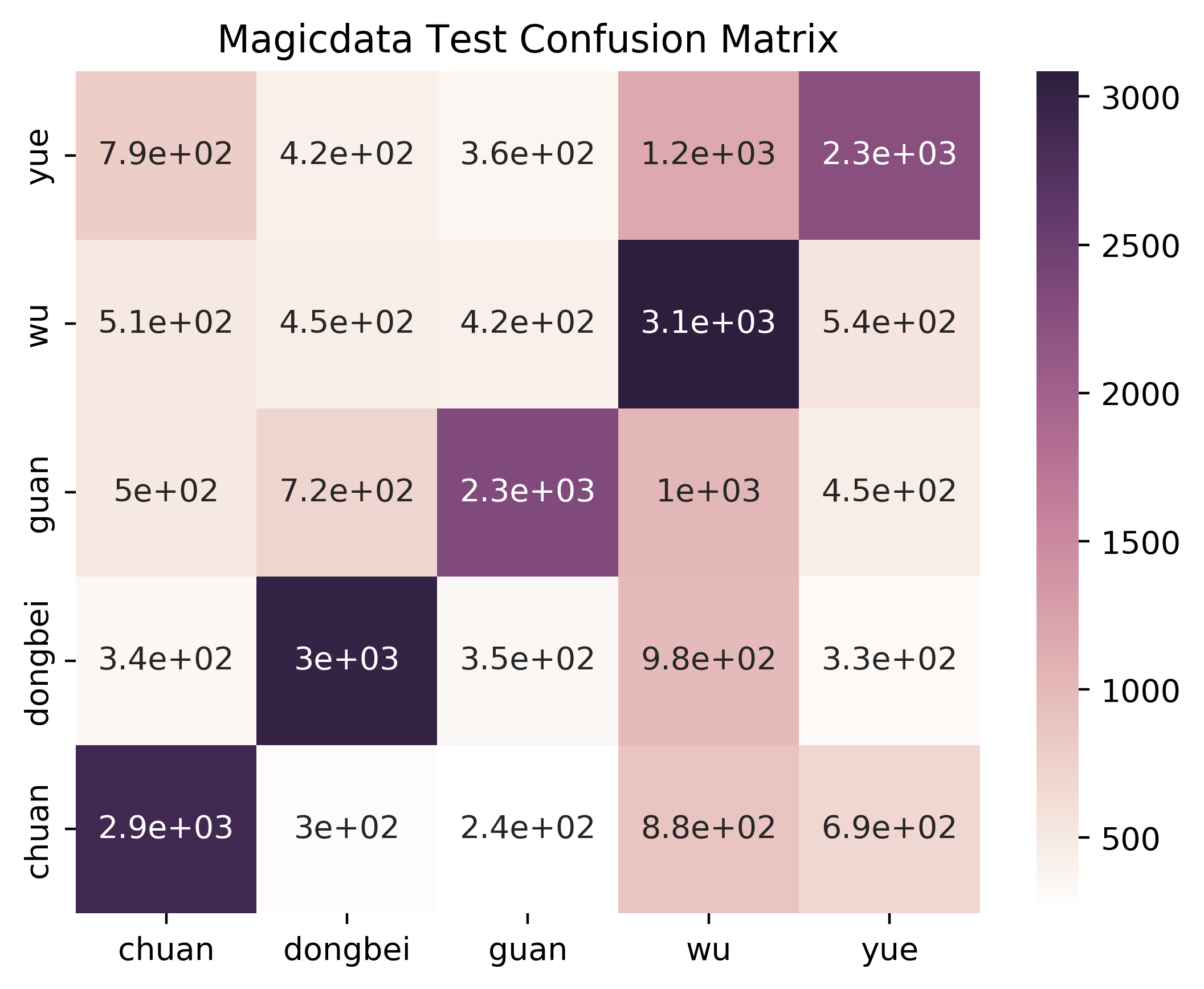
Figure 4: TDNN Classifier test confusion matrix

4.2.2 1D-CNN on Spectrogram

This section presents the implementation of the 1D-CNN classifier described in 3.1.2.

To train a 1D-CNN model, the input to the 1D-CNN must be of a predefined dimension and all input samples must have a predefined dimension. In the spectrogram data extracted, as described in 4.1.3, the frequency axis is fixed while the time dimension can vary depending on the original utterance length. To unify the time dimension, we trimmed the long utterances and padded the short ones. To determine the proper dimension for the time axis, the distribution of time length, as shown in Fig.5, was taken into consideration. In our model, we set the time dimension to $256$. For spectrogram with time longer than $256$, a random portion of dimension $256$ was taken out and the exceeding part was trimmed. Spectrogram with shorter duration than $256$, we padded them with zeros.

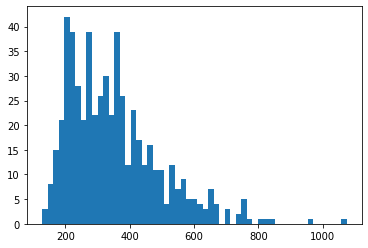
Figure 5: Time dimension distribution of spectrogram data

The layers of 1D-CNN for the MAGICDATA is summarized in 5.

Layer Type	Output Shape	Params #
Input	$[(None,256,129)]$	$0$
BatchNormalization	$(None,256,129)$	$516$
Conv1D	$(None,247,100)$	$129100$
Conv1D	$(None,238,100)$	$100100$
MaxPooling1D	$(None,79,100)$	$0$
BatchNormalization	$(None,79,100)$	$400$
Conv1D	$(None,70,160)$	$160160$
Conv1D	$(None,61,160)$	$256160$
GlobalAveragePooling	$(None,160)$	$0$
Dropout	$(None,160)$	$0$
Dense Softmax Output	$(None,5)$	$805$

Table 5: 1D-CNN Model for MAGICDATA Summary

Batch normalization helps prevent the network training from stagnating, due to the vanishing gradient problem and also provides a some regularization. Dropout layer was also introduced to regularize the training and to make the learning of the weights more robust. Callbacks and early stopping were introduced to prevent overfitting. The model training configuration is listed in table 6.

Experiments were carried out on both the Aishell-2 and MAGICDATA datasets. The dimension of the spectrogram at every timestamp was $129$, as specified before.

For the Aishell-2 dataset with $2$ classes, the data split details and training results are both illustrated in table 6. Due to the nature of the labels as described in 4.1.1, it is believed that the results may not be conclusive enough, on the effectiveness of the model. Therefore, experiment were carried out on the MAGICDATA.

For the MAGICDATA with $5$ classes, the data split details and training results are both illustrated in table 6 as well.

Training Configuration (for both datasets)	Aishell-2 Data Split	MAGICDATA Data Split
Number of epochs: $[20,30]$	Train set: $15672$ utterances (samples)	Train set: $12016$ utterances (samples)
Loss function: Categorical cross-entropy	Test set: $4472$ utterances (samples)	Test set: $3004$ utterances (samples)
Optimizer: Adam	Input shape: $(n,255,129)$	Input shape: $(n,256,129)$
Metric: Accuracy	Output shape: $(n,2)$	Output shape: $(n,5)$
-	Aishell-2 Training Results	MAGICDATA Training Results
-	Train accuracy: $90\%$	Train accuracy: $82\%$
-	Test accuracy: $87\%$	Test accuracy: $62\%$

Table 6: 1D-CNN Model data split, training configuration and results

Fig.6 shows the confusion matrix of the 1D-CNN on the test set, for the MAGICDATA dataset with $5$ classes. From the confusion matrix, it can be concluded that the 1D-CNN classifier performs best when classifying the guan accent, but has more trouble classifying the wu accent.

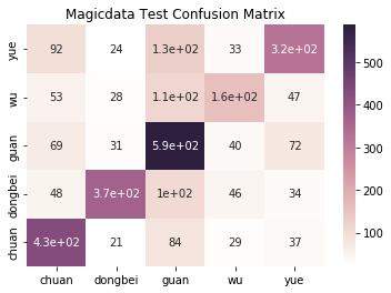
Figure 6: 1D-CNN Classifier test confusion matrix

4.2.3 Classifier Comparison

	TDNN	1D-CNN
	with MFCC	with Spectrogram
Train accuracy	$80\%$	$\bf{82\%}$
Test accuracy	$54\%$	$\bf{62\%}$
Best classified	dongbei, wu	guan
Worst classified	guan, yue	wu

Table 7: Comparison of TDNN Classifier with MFCC and 1D-CNN Classifier with Spectrogram on MAGICDATA

As illustrated in table 7, 1D-CNN classifier outperforms TDNN classifier, with a test accuracy of $62\%$. This can be because the TDNN classifier is trained with MFCC features, whereas the 1D-CNN classifier is trained using spectral features. Spectral features contain different information compared with MFCCs; specifically, spectrogram features contain pitch information whereas MFCC features do not. Since Chinese is a tonal language, pitch can be a key characteristics in differentiating different accents. This difference in feature attributes could be the essential reason why the 1D-CNN classifier outperforms the TDNN classifier.

Another difference worth noticing is that TDNN classifier performs the best on the wu accent, which 1D-CNN performs the worst on; whereas 1D-CNN performs the best on guan accent, which TDNN classifier performs the worst on. This could be caused by the similar issue mentioned above, which is that spectrogram features contain pitch information while MFCC features do not. From empirical experiences, the wu accent and guan accent (usually considered standard Mandarin) differ very little in tones, meaning both accents are featured with standard Mandarin tones. It is the other characteristics, such as differences in vowel and consonant pronunciation, that distinguish the two accents. Therefore, pitch information can be confounding when classifying the wu accent.

4.3 Accent Conversion

In the implementation of the accent conversion, spectrogram features were used. The two classifiers trained, as in 3.1, use MFCC features and spectrogram feature, respectively. As described in 3.2, the feature used in the accent conversion must have the property of being able to be converted to and from sampled audio. MFCCs features do not provide the best reconstruction, and thus are not as suitable for accent conversion. Therefore, in our accent converter prototype, spectrogram feature were used. Other features that may be reconstructed into audio form, such as Speex and CELP [11], are worth exploring in the future.

4.3.1 Data Processing

The first step of data processing was to unify the input spectrogram dimension by trimming the long ones and padding the short ones, as described earlier in 4.2.2. Since the classifier model is part of the accent conversion trainer model, all the data processing for the classifier and the converter must be identical. For all the accent conversion experiments presented, the same data processing steps were taken out and the classifier and the accent converter were then trained on the same processed dataset.

The first few experiments were conducted on the raw spectrogram (after unifying the dimension) without transforming the data. The classifier performed similarly regardless of whether log and exponential transformations and standardization were performed or not. On the other hand, both the encoder and the decoder failed to learn on the raw spectrogram (after unifying the dimension). The training suffered from vanishing/exploding gradients.

The log-exponential spectrogram transformation presented in [16] was then implemented. The spectrogram was first log-transformed, standardized, and then fed to the encoder. The output from the decoder was destandardized, and then transformed exponentially to retrieve the value of the scale before transformation. The log-exponential transformation in the implementation was based on the method in [16], with the only difference of adding a small offset to prevent 0’s in the logarithms. With this transformation and the use of batch normalization, the model trained properly, without experiencing any exploding/vanishing gradients.

4.3.2 Training

The initial attempt was to train the encoder and the decoder separately, different from the training method described in 3.2.1. To train the encoder and the decoder separately, two separate trainers were built. The first trainer was the encoder trainer, where the encoder was connected to the fixed-weight classifier. The encoder trainer had one input and one output as follows,

• Input 1: encoder input – original accented speech in the feature space

• Output 1: classifier output – probability of the speech containing each accent, as a vector

The decoder trainer was the trained encoder connected to the decoder, which was also the final converter model. The weights of the trained encoder were fixed and only the decoder was trained. The decoder trainer was also the converter, with two inputs and one output, as shown below.

• Input 1: encoder input – original accented speech in the feature space

• Input 2: decoder input 2 – original accent label in one-hot format

• Output 1: decoder output – converted accented speech in the feature space

With this technique of separating the training for the encoder and the decoder, the converter did not perform well. In fact, the encoder output produced parallel lines in the spectrogram, which was undesirable, as it would not even preserve the content, let alone being an accent-neutral representation of speech. The decoder naturally failed because the decoder was based on the encoder’s output. The reason for the encoder learning a very lossy conversion and outputting parallel lines could be that in this encoder trainer model, the only output was the classifier output. In other words, the loss incurred by the classifier output was the source of the overall loss that solely guided the model’s learning. The encoder would reach a very low loss as long as the output could make the classifier output a uniform classification prediction, without having to preserve the speech information. To ensure that the encoder’s output would preserve the speech content and that it would be accent-neutral, the encoder and the decoder should be trained together, as described in 3.2.1. This way, both of the two output losses (the classifier and the decoder output) would contribute to the overall loss and collectively guide the model’s learning. This can prevent the issue previously encountered, when the encoder and the decoder were trained separately. The training setting for the converter trainer model on MAGICDATA dataset is provided here,

• Loss for classifier output: categorical crossentropy

• Loss for decoder output: binary crossentropy

• Number of epochs: in range $[20,30]$

• Batch size: $128$

• Train set size: $12016$

• Test set size: $3004$

4.3.3 Latent Dimension

Another experiment was performed on the encoder and the decoder model structure. In this case, the intermediate result (encoder output) had the same dimension as the encoder input and the decoder output, as it is an accent-neutral representation of the speech in the same feature space (s.t. it can be fed to the accent classifier). This makes it very different from traditional autoencoder architectures, where the introduction of a bottleneck latent dimension is key to forcing a compressed knowledge representation of the original input and does not just naively play the role of normalizing the input and of passing the values through. We experimented with replacing both the encoder model and the decoder model with an autoencoder architecture, where a latent dimension was introduced. However, there did not appear to be any significant improvement to warrant the benefit of this architecture in our experiment. Eventually, the encoder-decoder without any latent dimension was used.

4.3.4 Converter Architecture

The best accent converter model in our experiment was an encoder-decoder model trained on the MAGICDATA dataset. The architecture of this model is shown in Table 8, Table 9, and Table 10. Table 8 shows the encoder model architecture.

Layer Type	Output Shape	Params #
Input	$[(None,256,129)]$	$0$
BatchNormalization	$(None,256,129)$	$516$
Conv1D	$(None,256,160)$	$206560$
Conv1D	$(None,256,160)$	$256160$
BatchNormalization	$(None,256,160)$	$640$
Conv1D	$(None,256,160)$	$256160$
Conv1D	$(None,256,160)$	$256160$
MaxPooling1D	$(None,32,160)$	$0$
BatchNormalization	$(None,32,160)$	$640$
Dropout	$(None,32,160)$	$0$
Conv1D	$(None,32,100)$	$160100$
Conv1D	$(None,32,100)$	$100100$
Upsampling1D	$(None,256,100)$	$0$
BatchNormalization	$(None,256,100)$	$400$
Conv1D	$(None,256,129)$	$129129$

Table 8: Encoder Model for MAGICDATA Summary

Table 9 shows the decoder model layers and Table 10 shows the connection architecture.

Layer Type	Output Shape	Params #
Input1(Spectrogram)	$[(None,256,129)]$	$0$
Input2(Label)	$[(None,5)]$	$0$
Embedding	$(None,5,129)$	$258$
Concatenante	$(None,261,129)$	$0$
Conv1D-1	$(None,261,160)$	$206560$
Conv1D-2	$(None,261,160)$	$256160$
MaxPooling1D	$(None,32,160)$	$0$
BatchNormalization-1	$(None,32,160)$	$640$
Conv1D-3	$(None,32,100)$	$160100$
Conv1D-4	$(None,32,100)$	$100100$
Dropout	$(None,32,100)$	$0$
Upsampling1D	$(None,256,100)$	$0$
BatchNormalization-2	$(None,256,100)$	$400$
Conv1D	$(None,256,129)$	$129129$

Table 9: Decoder Model for MAGICDATA Layers

Layer Type	Connected To
Input1(Spectrogram)	-
Input2(Label)	-
Embedding	Input2
Concatenante	Input1 + Embedding
Conv1D-1	Concatenante
Conv1D-2	Conv1D-1
MaxPooling1D	Conv1D-2
BatchNormalization-1	MaxPooling1D
Conv1D-3	BatchNormalization-1
Conv1D-4	Conv1D-3
Dropout	Conv1D-4
Upsampling1D	Dropout
BatchNormalization-2	Upsampling1D
Conv1D	BatchNormalization-2

Table 10: Decoder Model for MAGICDATA Connections

4.3.5 Converter in Action

Some sample accent conversions were run using the accented speech and its corresponding accent class label as input. The ideal output of the accent converter wold be the reconstruction of the input accented speech. This experiment was performed with the encoder-decoder converter trained with $5$ accent classes of MAGICDATA.

Fig.7 shows the comparison between the original input spectrogram and the accent-converted spectrogram using the original input’s accent label, where the left side shows the original spectrograms and the right side shows their corresponding converted spectrograms (reconstructed via the converter). As apparent in Fig.7, output spectrogram resembles the input. The output preserving most of the lower frequencies while losing details mostly in the higher frequencies.

It is helpful to also look at the waveform of the speech input and output. Fig.8 shows the comparison between the original input waveform and the accent-converted waveform, using the original input’s accent label, where the left side shows the original waveforms and the right side shows their corresponding converted (reconstructed via the converter) waveforms. It is clear from Fig.8 that although the overall shape is similar, the converted speech loses quite a bit of the detail, present in the input.

The discovery from listening to the audio form of the sample accent conversions is consistent with the visual representation. The converted audio preserves the tone and intonation of the input while the details are blurred.

A study on multi-target voice conversion without parallel data by Chou, Yeh, Lee, and Lee [17] describes similar issues of blurred output from the decoder and presents a solution. From their insights, it is believed that the issue of losing details from the decoder output may be addressed by the introduction of a cycle-GAN model. We plan to pursue this approach in order to resolve this issue of loss of details in the decoder output, a more detailed proposal of future work to tackle this issue will be discussed in 5.2.

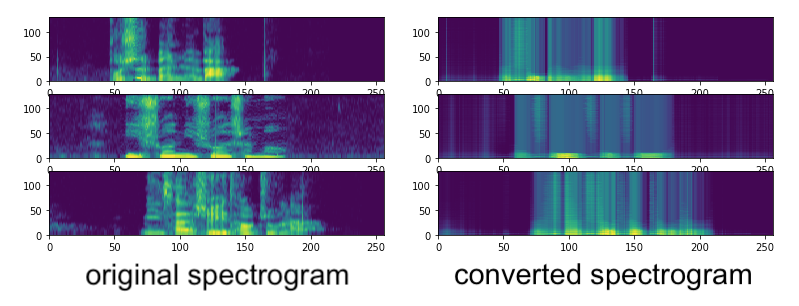
Figure 7: Original and converted spectrograms comparison

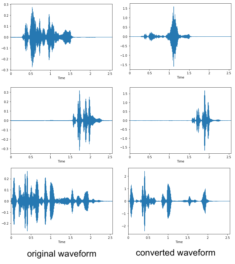
Figure 8: Original and converted waveforms comparison

5 Conclusions and Future Work

At this point some conclusions based on our new architecture and approach are presented, followed by what will be pursued in some of our future research.

5.1 Conclusions

As shown in Section 4.2.3, the 1D-CNN classifier experiment outperforms the TDNN version. However, this is most likely due to the use of spectral features in the 1D-CNN case, which contain pitch information. Since Chinese is a tonal language, pitch information can be a key characteristics in distinguishing regional accents. In addition, pitch, in any language defines the major variations in accents.

As mentioned in Section 4.3.5, converted speech output from our converter model loses some details when compared with the original spectrogram and waveform. By listening to the generated audio, it is ascertained that the converted audio preserves the tones and intonation of the original audio, but details are blurred. This is a common issue with speech and audio generation, and needs further improvement. One possible solution is described in Section 5.2. Being able to preserve tones and intonation indicates that our converter model might perform better on accents with distinctive tones and intonation. This means that it might produce better conversion results if the original accent and desired accent have very different tones and intonation.

5.2 Future Work

In this section, we propose some of the experiments we may possibly carry out in the future in order to improve our models.

5.2.1 cycle-GAN for Decoder Output Refinement

As mentioned above, our converter model managed to preserve tones and intonation during the conversion, but it blurred out the details. Therefore, it is worth trying to tackle this issue using the approach proposed by Chou, Yeh, Lee, and Lee [17]. This study on multi-target voice conversion describes similar issues of blurred output from the decoder and presents a solution. We believe that the issue of losing details from the decoder output may be addressed by the introduction of a cycle-GAN model.

5.2.2 Transfer Learning on Spectrogram Features

Even though, currently, our 1D-CNN model outperforms the TDNN model trained through transfer learning, we still believe that pre-trained x-vector speaker recognition model might contain accent information, and can be used for accent recognition. As discussed above, Chinese is a tonal language, but MFCC features do not carry pitch information. Therefore, one possible way to improve the TDNN model is to combine pitch features with MFCC features, and/or use spectrogram features during training.

As indicated by the results presented in Table 7, the Spectrogram and MFCC features seem to provide complementary results when it comes to classifying the different accents. Therefore, it seems quite plausible that combining the MFCC with spectral features would increase the accuracy of the underlying system. In that regard, the pitch may also be added to the set.

5.2.3 Alternative Features

One of the reasons why spectrogram features are of interest is that they can be easily converted back to waveform, whereas there is currently no simple and well-performing approach of generating waveform with MFCC. From this aspect, we could also try to explore some other features, such as CELP encoding, that can be easily extracted/encoded and converted back/decoded to waveform. Such features contain more information as well, which might possibly improve our model performance.

References

- [1] S. Aryal and R. Gutierrez-Osuna, “Articulatory-based conversion of foreign accents with deep neural networks,” in INTERSPEECH, 2015.
- [2] A. Bearman, K. Josund, and G. Fiore, “Accent conversion using artificial neural networks,” Stanford University, Tech. Rep, Tech. Rep., 2017.
- [3] H. Beigi, Fundamentals of Speaker Recognition. New York: Springer, 2011, iSBN: 978-0-387-77591-3.
- [4] G. Zhao, S. Ding, and R. Gutierrez-Osuna, “Foreign accent conversion by synthesizing speech from phonetic posteriorgrams,” Proc. Interspeech 2019, pp. 2843–2847, 2019.
- [5] S. Mobin and J. Bruna, “Voice conversion using convolutional neural networks,” arXiv preprint arXiv:1610.08927, 2016.
- [6] S. H. Mohammadi and A. Kain, “Voice conversion using deep neural networks with speaker-independent pre-training,” in 2014 IEEE Spoken Language Technology Workshop (SLT). IEEE, 2014, pp. 19–23.
- [7] Y. Jiao, M. Tu, V. Berisha, and J. M. Liss, “Accent identification by combining deep neural networks and recurrent neural networks trained on long and short term features.” in Interspeech, 2016, pp. 2388–2392.
- [8] S. P. Hernandez, V. Bulitko, S. Carleton, A. Ensslin, and T. Goorimoorthee, “Deep learning for classification of speech accents in video games.” in AIIDE Workshops, 2018.
- [9] Y. Zheng, R. Sproat, L. Gu, I. Shafran, H. Zhou, Y. Su, D. Jurafsky, R. Starr, and S.-Y. Yoon, “Accent detection and speech recognition for shanghai-accented mandarin,” in Ninth European Conference on Speech Communication and Technology, 2005.
- [10] D. Snyder, D. Garcia-Romero, G. Sell, D. Povey, and S. Khudanpur, “X-vectors: Robust dnn embeddings for speaker recognition,” in 2018 IEEE International Conference on Acoustics, Speech and Signal Processing (ICASSP). IEEE, 2018, pp. 5329–5333.
- [11] J.-M. Valin, “Introduction to celp coding,” Manual, 2010. [Online]. Available: http://speex.org/docs/manual/speex-manual/manual.html
- [12] J. Du, X. Na, X. Liu, and H. Bu, “Aishell-2: Transforming mandarin asr research into industrial scale,” arXiv preprint arXiv:1808.10583, 2018.
- [13] MAGICDATA Mandarin Chinese Read Speech Corpus, Magic Data Technology Co., May 2019, available at http://www.openslr.org/68/.
- [14] M. Morise, F. Yokomori, and K. Ozawa, “World: a vocoder-based high-quality speech synthesis system for real-time applications,” IEICE TRANSACTIONS on Information and Systems, vol. 99, no. 7, pp. 1877–1884, 2016.
- [15] S. Ioffe, “Probabilistic linear discriminant analysis,” in Computer Vision – ECCV 2006, A. Leonardis, H. Boschof, and A. Pinz, Eds. Springer, 2006, pp. 531–542.
- [16] C.-C. Hsu, H.-T. Hwang, Y.-C. Wu, Y. Tsao, and H.-M. Wang, “Voice conversion from non-parallel corpora using variational auto-encoder,” in 2016 Asia-Pacific Signal and Information Processing Association Annual Summit and Conference (APSIPA). IEEE, 2016, pp. 1–6.
- [17] J.-c. Chou, C.-c. Yeh, H.-y. Lee, and L.-s. Lee, “Multi-target voice conversion without parallel data by adversarially learning disentangled audio representations,” arXiv preprint arXiv:1804.02812, 2018.