Infeasibility and error bound imply finite convergence of alternating projections

Abstract

This paper combines two ingredients in order to get a rather surprising result on one of the most studied, elegant and powerful tools for solving convex feasibility problems, the method of alternating projections (MAP). Going back to names such as Kaczmarz and von Neumann, MAP has the ability to track a pair of points realizing minimum distance between two given closed convex sets. Unfortunately, MAP may suffer from arbitrarily slow convergence, and sublinear rates are essentially only surpassed in the presence of some Lipschitzian error bound, which is our first ingredient. The second one is a seemingly unfavorable and unexpected condition, namely, infeasibility. For two non-intersecting closed convex sets satisfying an error bound, we establish finite convergence of MAP. In particular, MAP converges in finitely many steps when applied to a polyhedron and a hyperplane in the case in which they have empty intersection. Moreover, the farther the target sets lie from each other, the fewer are the iterations needed by MAP for finding a best approximation pair. Insightful examples and further theoretical and algorithmic discussions accompany our results, including the investigation of finite termination of other projection methods.

47N10, 49M27, 65K05, 90C25

1 Introduction

The method of alternating projections (MAP) has a remarkable impact in so many areas of Mathematics and is one of the main classical tools for solving convex feasibility problems. A broad class of problems in Applied Mathematics is effectively solved by MAP [34]. Definitely one of a kind, MAP is not only capable of tracking a point in the intersection of given closed convex sets $X,Y\subset\mathds{R}^{n}$, it delivers a replacement of an actual solution when $X$ and $Y$ do not intersect. Such a replacement comes in the form of a pair $(\bar{x},\bar{y})\in X\times Y$, often called best approximation pair to $X$ and $Y$, as it minimizes the Euclidean distance between these two sets.

It is well-known that MAP converges globally whenever the distance between $X$ and $Y$ is attainable. It is also worth mentioning that, in view of Pierra’s famous product space reformulation [48], feasibility problems involving a finite number of sets can be narrowed down to seeking a common point to two sets $X$ and $Y$.

The present work focuses on the inconsistent case $X\cap Y=\emptyset$ and reveals a surprising behavior of MAP in this setting. Roughly speaking, we come to the conclusion that infeasibility works in favor of MAP. Quite intuitive when looking at the scenarios displayed in Figure 1, the fact that infeasibility has a strong positive impact on MAP has apparently not been seen anywhere in its extensive literature. Actually, we prove that infeasibility added by an error bound condition provides finite convergence of the very pure MAP. More precisely, by assuming $X\cap Y=\emptyset$ and a suitable error bound condition, we prove finite convergence of the MAP sequence defined by $x^{k+1}\coloneqq P_{X}P_{Y}(x^{k})$ starting at any point $x^{0}\in\mathds{R}^{n}$. Finite convergence means that for some non-negative integer $\bar{k}$, MAP reaches a best point $\bar{x}\in X$, that is, $x^{\bar{k}}=\bar{x}$ and $\bar{y}=P_{Y}(\bar{x})$ form a best approximation pair to $X$ and $Y$. Here and throughout the text, $P_{X}$ and $P_{Y}$ stand for the orthogonal projections onto $X$ and $Y$, respectively.

Let us now look at a collection of illustrations that serves as a summary of our results.

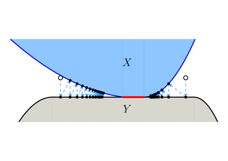
(a) figure]fig:MAPfigure1a Consistency; linear convergence on the left.

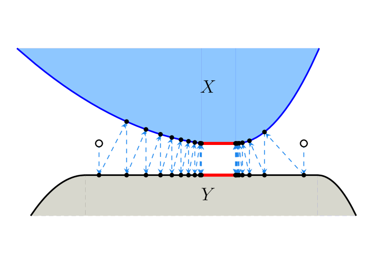
(b) figure]fig:MAPfigure1b Inconsistency; $k=10$ on the left.

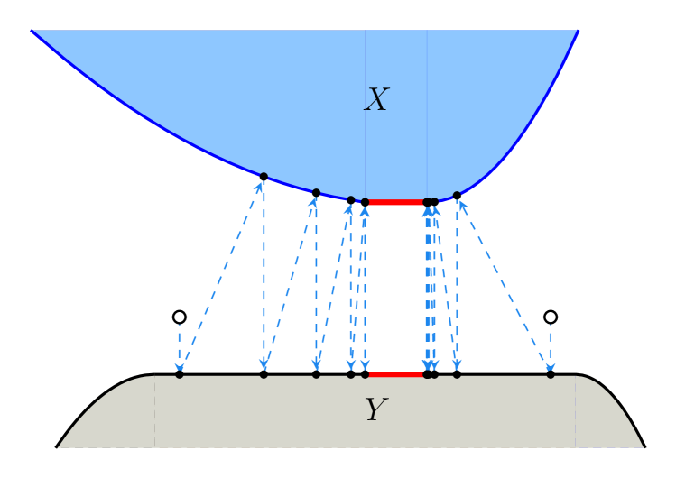
(c) Inconsistency; increasing the distance between $X$ and $Y$; $k=5$ on the left.figure]fig:MAPfigure1c

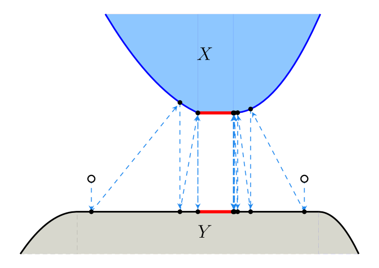
(d) Inconsistency; improving the error bound on the left; $k=3$ on the left.figure]fig:MAPfigure1d

Figure 1: Error bound on the left-hand sides.

Figure 1 displays four scenarios of MAP acting on sets $X$ and $Y$. We start with a consistent problem in LABEL:fig:MAPfigure1a and analyze two MAP sequences. The one starting from the left converges linearly to a point in $X\cap Y$. This is due to the fact that in this region $X$ and $Y$ form a non-zero angle. In other words, a Lipschitzian error bound holds. This is not the case on the right-hand side of the picture and therefore, MAP only achieves sublinear convergence over there. By lifting $X$, we generate inconsistent intersection problems in LABEL:fig:MAPfigure1b, LABEL:fig:MAPfigure1c, and LABEL:fig:MAPfigure1d. The result is that MAP responds favorably speed-wise to this translation of $X$. More than that, MAP improves when increasing infeasibility and also when the error bound gets better, that is, the left border of $X$ gets steeper. This can be noticed looking at Figure 1 as a film from LABEL:fig:MAPfigure1a, LABEL:fig:MAPfigure1b, LABEL:fig:MAPfigure1c, and LABEL:fig:MAPfigure1d. Lifting $X$ from LABEL:fig:MAPfigure1a to LABEL:fig:MAPfigure1b makes MAP’s convergence jump from linear to finite on the left. On the right-hand side, MAP leaps its convergence rate from sublinear to linear. After a further lift of $X$ from LABEL:fig:MAPfigure1b to LABEL:fig:MAPfigure1c, MAP reaches a best point in $5$ iterations instead of $10$ on the left-hand side. MAP only needs $3$ iterates to get a best approximation pair when improving the error bound in the left part of LABEL:fig:MAPfigure1d.

The message of Figure 1 is fairly clear. As for the aforementioned error bound condition, it will be formally introduced later. We anticipate, though, that it regards the target sets and their relation with what we are going to call optimal supporting hyperplanes. We point out that such an error bound is automatically globally fulfilled if $X$ is a polyhedron and $Y$ a hyperplane, providing finite convergence of MAP if, in addition, these particular polyhedral sets have empty intersection. Note that finite convergence of MAP may happen even under a non-polyhedral structure, as depicted in Figure 1.

Before outlining the structure of our paper, we briefly go through some turning points in the history of MAP. This method has fascinated scientists for nearly a century now, and although many results on this simple tool have been derived, open questions remain. In the early 1930s, von Neumann firstly studied MAP for subspaces. Yet, his results were only published in 1950 [51], proving the convergence of MAP to a so-called best approximation solution for the intersection of two subspaces. In 1937, Kaczmarz [43] proposed a MAP related algorithm (also known as Cyclic projections) for finding best approximation solutions of linear systems. In 1959, MAP was studied for the convex case by Cheney and Goldstein [28], covering also inconsistent feasibility problems. Precisely the theme of our paper, projection methods for inconsistent inclusions have a history on their own; see the 2018 review by Censor and Zaknoon [27]. The ability of MAP to find best approximation pairs is a notable characteristic, making MAP (and its variants) one of the most used algorithms in Optimization [35, 36, 30, 8, 24, 37, 9, 50, 17, 33, 1]. Although MAP always converges under the existence of best approximation pairs, the convergence rate may be arbitrarily slow [16, 6, 41]. In 1950, Aronszajn [4] found the lower bound for the linear rate of MAP, given by the square of the cosine of the minimal angle (Friedrichs angle) between two subspaces, which turns out to be the sharpest one, as proved by Kayalar and Weinert [44] in 1988. For an in depth related literature on MAP; see, for instance, Bauschke and Borwein [10, 12], and Deutsch [34].

The paper is organized as follows. In Section 2 we collect known facts on MAP and some auxiliary material. Section 3 contains our mayor results concerning the geometry of two disjoint closed convex sets in the presence of an error bound condition. This analysis allows us to derive in Section 4 our main result, namely, finite convergence of MAP under inconsistency and what we call BAP error bound. The BAP error bound is automatically fulfilled for a polyhedron and a hyperplane, and we study its connection with linear regularity and intrinsic transversality. Also in Section 4, we will see that for a MAP sequence to converge in a finite number of steps, it is necessary and sufficient that it satisfies the BAP error bound at its iterates. Section 4 ends by investigating finite termination under inconsistency of Cyclic projections, Cimmino and Douglas-Rachford methods. In Section 5, we present insightful examples and applications. In particular, we connect our results to Linear Programming and convex min-max problems. We consider as well a simple problem giving rise to the question on whether a Hölder type error bound could make MAP’s rate of convergence go from sublinear to linear when shifting the target sets apart. Some concluding remarks are presented in Section 6.

2 Background material

Let $X,Y\subset\mathds{R}^{n}$ be closed, convex and nonempty. We recall that the orthogonal projection of $x\in\mathds{R}^{n}$ onto $X$ is given by $P_{X}(x)\in X$ if, and only if, $\left\langle{y-P_{X}(x)},{x-P_{X}(x)}\right\rangle\leq 0,$ for all $y\in X$. Throughout the text, $\left\langle{\cdot},{\cdot}\right\rangle$ stands for the Euclidean inner product inducing the norm $\left\lVert\cdot\right\rVert\coloneqq\sqrt{\left\langle{\cdot},{\cdot}\right\rangle}$. The non-negative integer numbers will be denoted by $\mathds{N}$. The open ball centered in $x$ with radius $\delta>0$ is the set $\mathscr{B}_{\delta}(x)\coloneqq\{z\in\mathds{R}^{n}\mid\left\lVert x-z\right\rVert<\delta\}$.

We define the distance between $X$ and $Y$ by $\operatorname{dist}(X,Y)\coloneqq\inf\{\left\lVert x-y\right\rVert\mid x\in X,y\in Y\}.$ When one of the sets is a singleton, for instance $X=\{x\}$, we use the notation $\operatorname{dist}(x,Y)$. A best approximation pair (BAP) relative to $X$ and $Y$ is a pair $(\bar{x},\bar{y})\in X\times Y$ attaining the distance between $X$ and $Y$, that is, $\operatorname{dist}(\bar{x},\bar{y})=\operatorname{dist}(X,Y)$. The set of all BAP relative to $X$ and $Y$ is denoted by $\operatorname{bap}(X,Y)\subset X\times Y$ and, accordingly, we define the sets

$$\operatorname{bap}_{Y}(X)\coloneqq\{x\in X\mid(x,y)\in\operatorname{bap}(X,Y)\}=\{x\in X\mid\operatorname{dist}(x,Y)=\operatorname{dist}(X,Y)\}$$

and

$$\operatorname{bap}_{X}(Y)\coloneqq\{y\in Y\mid(x,y)\in\operatorname{bap}(X,Y)\}=\{y\in Y\mid\operatorname{dist}(y,X)=\operatorname{dist}(X,Y)\}.$$

Note that $\operatorname{bap}_{Y}(X)$ (respectively $\operatorname{bap}_{X}(Y)$) is the subset of points in $X$ (respectively $Y)$ nearest to $Y$ (respectively $X$). In the consistent case, that is, when $X\cap Y$ is nonempty, we have $\operatorname{bap}_{X}(Y)=\operatorname{bap}_{Y}(X)=X\cap Y$. As we are interested in the inconsistent case, henceforth, we suppose that $X\cap Y=\emptyset$. In this context we define the displacement vector as $d\coloneqq P_{\operatorname{cl}(X-Y)}(0).$ So, $\left\lVert d\right\rVert=\operatorname{dist}(X,Y)$ and $\operatorname{dist}(X,Y)$ is attained if, and only, if $d\in X-Y$. In particular, $\operatorname{dist}(X,Y)$ is attained whenever $X-Y$ is closed.

Given any point $x\in\mathds{R}^{n}$, define the terms of the sequence $(x^{k})_{k\in\mathds{N}}$ by

$$x^{0}=x,\quad x^{k+1}=P_{X}P_{Y}(x^{k}),$$

for every $k\in\mathds{N}$. The sequence $(x^{k})_{k\in\mathds{N}}$ is the alternating projection sequence starting at $x^{0}=x$. Cheney and Goldstein established in [28] that if one of the sets is compact or if one of the sets is finitely generated, the fixed point set of the operator $P_{X}P_{Y}$ is nonempty and the sequence Section 2 converges to a fixed point of this operator. The general result was summarized and enlarged in [11] as follows.

Fact 1 (BAP sets [11, Lemma 2.2]).

Denote $\operatorname{Fix}(P_{X}P_{Y})=\{x\in\mathds{R}^{n}\mid P_{X}P_{Y}(x)=x\}$. Then,

1. $\operatorname{bap}_{Y}(X)=\operatorname{Fix}(P_{X}P_{Y})$.

2. $\operatorname{bap}_{Y}(X)$ and $\operatorname{bap}_{X}(Y)$ are closed convex sets.

3. If $\operatorname{bap}_{Y}(X)$ or $\operatorname{bap}_{X}(Y)$ is nonempty then $\operatorname{dist}(X,Y)$ is attained. Moreover, let $d$ be the displacement vector. Then

   $$P_{Y}(\bar{x})=\bar{x}-d,\quad\forall\bar{x}\in\operatorname{bap}_{Y}(X),$$

   and $\operatorname{bap}_{Y}(X)-d=\operatorname{bap}_{X}(Y),\operatorname{bap}_{Y}(X)=X\cap(Y+d),\operatorname{bap}_{X}(Y)=(X-d)\cap Y.$

In the next fact, we abuse notation and use $\left\langle{X},{y}\right\rangle\leq 0$ to denote that $\left\langle{x},{y}\right\rangle\leq 0,\forall x\in X$.

Fact 2 (BAP pairs).

Let $x\in\mathds{R}^{n}$ be given. Then, if $\operatorname{dist}(X,Y)$ is attained, with $d$ being the displacement vector, then

$$P_{\operatorname{bap}_{X}(Y)}(x)=P_{\operatorname{bap}_{Y}(X)}(x)-d,$$

and $\langle X-\operatorname{bap}_{Y}(X),d\rangle\geq 0$ and $\langle Y-\operatorname{bap}_{X}(Y),d\rangle\leq 0$.

Fact 3 (Convergence of MAP [11, Theorem 4.8]).

Let $(x^{k})_{k\in\mathds{N}}$ be an alternating projection sequence as given in Section 2. Then,

$$x^{k}-P_{Y}(x^{k})\to d,$$

where $d$ is the displacement vector. Moreover,

1. if $\operatorname{dist}(X,Y)$ is attained then $x^{k}\to\bar{x}\in\operatorname{bap}_{Y}(X)$ and $P_{Y}(x^{k})\to\bar{y}\coloneqq\bar{x}-d\in\operatorname{bap}_{X}(Y)$;

2. if $\operatorname{dist}(X,Y)$ is not attained then $\left\lVert x^{k}\right\rVert\to+\infty$.

Next we present some definitions and well-known results concerning polyhedra, useful in Lemmas 3.1 and 4.1.

Definition 2.1 (Polyhedron).

A set $\Omega\subset\mathds{R}^{n}$ is said to be a polyhedron, if it can be expressed as the intersection of a finite family of closed half-spaces, that is,

$$\Omega\coloneqq\{x\in\mathds{R}^{n}\mid\left\langle{a_{i}},{x}\right\rangle\leq\alpha_{i},\text{ for }i=1,\ldots,m\},$$

where $a_{i}\in\mathds{R}^{n},\alpha_{i}\in\mathds{R}$.

Note that a polyhedron, also referred to as a polyhedral set, is always convex.

Definition 2.2 (Finitely generated cone and conic base).

A set $K\subset\mathds{R}^{n}$ is a cone if it is closed under positive scalar multiplication. A cone $K$ is finitely generated if there exists a finite set $S\subset\mathds{R}^{n}$ such that $\operatorname{cone}(S)=K$, where $\operatorname{cone}(S)$, is the set of all conic combinations of elements of $S$. A conic base of a finitely generated cone $K$ is a finite set $B_{K}\subset\mathds{R}^{n}$ with minimal cardinality such that $\operatorname{cone}(B_{K})=K$.

Fact 4 (Polyhedron is finitely generated [20, Proposition B.17]).

A set $\Omega\subset\mathds{R}^{n}$ is polyhedral if, and only if, it is finitely generated, i.e., there exist a nonempty and finite set of vectors $\left\{v_{1},\ldots,v_{m}\right\},$ and a finitely generated cone $K$ such that

$$\Omega=\{x\in\mathds{R}^{n}\mid x=y+\sum_{j=1}^{m}\mu_{j}v_{j},y\in K,\sum_{j=1}^{m}\mu_{j}=1,\mu_{j}\geq 0,j=1,\ldots,m\}.$$

Let us note that finitely generated cones are the same as polyhedral cones, because of the well-known Minkowski-Weyl Theorem [49, Theorem 3.52].

Definition 2.3 (Tangent and Normal cones).

Let $X$ be a nonempty closed convex set in $\mathds{R}^{n}$ and $x\in X$. The tangent cone of $X$ at $x$ is given by

$$\mathscr{T}_{X}(x)\coloneqq\operatorname{cl}\left(\left\{\lambda(y-x)\in\mathds{R}^{n}\mid y\in X,\lambda\in\mathds{R}_{+}\right\}\right).$$

The normal cone of $X$ at $x$ is the set defined by

$$\mathscr{N}_{X}(x)\coloneqq\left\{y\in\mathds{R}^{n}\mid\left\langle{y},{z-x}\right\rangle\leq 0,z\in X\right\}.$$

Fact 5 (Tangent cone of polyhedron [49, Theorem 6.46]).

If $\Omega\subset\mathds{R}^{n}$ is a polyhedron defined as in Definition 2.1, then the tangent cone $\mathscr{T}_{\Omega}(x)$, at any point $x\in\Omega$, is a polyhedral cone and can be represented as

$$\mathscr{T}_{\Omega}(x)=\{w\in\mathds{R}^{n}\mid\left\langle{a_{i}},{w}\right\rangle\leq 0,\text{ for }i\in\mathscr{I}(x)\},$$

where $a_{i}\in\mathds{R}^{n}$ defines the polyhedron $\Omega$ and $\mathscr{I}(x)\coloneqq\{i\mid\left\langle{a_{i}},{x}\right\rangle=\alpha_{i}\}$ is the active index set of $\Omega$ at $x$.

Fact 6 (Finitely many tangent cones of a polyhedron [20]).

If $\Omega$ is a polyhedron, then the set of all tangent cones $\{\mathscr{T}_{\Omega}(x)\mid x\in\Omega\}$ has finite cardinality. Moreover, for any $x\in\Omega$, there exists a radius $\delta>0$ such that $(\mathscr{T}_{\Omega}(x)+x)\cap\mathscr{B}_{\delta}(x)=\Omega\cap\mathscr{B}_{\delta}(x)$, that is, $\Omega$ coincides locally with any shifted tangent cone to it.

Finally, it is noteworthy that the distance between two non-intersecting polyhedral sets is attained.

Fact 7 (Distance between polyhedra is attained [28, Theorem 5]).

Let $\Omega_{1},\Omega_{2}\subset\mathds{R}^{n}$ be nonempty polyhedra with $\Omega_{1}\cap\Omega_{2}=\emptyset$. Then, $\operatorname{dist}(\Omega_{1},\Omega_{2})$ is attained.

3 On the geometry of two disjoint convex sets under error bound condition

This section is divided in two subsections, gathering key contributions of our paper. In the first subsection, we investigate the geometry under which a single alternating projection step reaches a best approximation pair when the sets are apart from each other. In the second one, we compare well-known regularity conditions from the literature with our proposed error bound.

3.1 BAP-EB and alternating projection step

Here we start stating that a single alternating projection step yields a best approximation pair to a polyhedron $\Omega$ and a hyperplane $H$, if $\Omega\cap H=\emptyset$ and the alternating projection step is taken from a point sufficiently close to $\operatorname{bap}_{H}(\Omega)$.

Lemma 3.1 (Alternating projection step for polyhedron versus hyperplane under inconsistency).

Consider two nonempty sets $\Omega,H\subset\mathds{R}^{n}$ such that $\Omega$ is a polyhedron, $H$ is a hyperplane and $\Omega\cap H=\emptyset$. Then, there exists a radius $r>0$ such that

$$P_{\Omega}P_{H}(z)\in\operatorname{bap}_{H}(\Omega),$$

for all $z\in\mathds{R}^{n}$ satisfying $\operatorname{dist}(z,\operatorname{bap}_{H}(\Omega))\leq r$.

Proof 3.2.

For a point $x\in\Omega$, let $\mathscr{T}_{\Omega}(x)$ denote the tangent cone of $\Omega$ at $x$. Since $\Omega$ is a polyhedron, the set of all tangent cones $\{\mathscr{T}_{\Omega}(x)\mid x\in\Omega\}$ is finite and each $\mathscr{T}_{\Omega}(x)$ is a finitely generated cone (see Facts 4, 5, and 6). In particular, the cardinality of $\Gamma\coloneqq\{\mathscr{T}_{\Omega}(x)\mid x\in\operatorname{bap}_{H}(\Omega)\}$ is finite since $\operatorname{bap}_{H}(\Omega)\subset\Omega$ and each tangent cone in $\Gamma$ has a finite number of generators. Consider now the collection of all normalized generators with respect to cones in $\Gamma$ denoted by $W\coloneqq\{w\in\mathds{R}^{n}\mid\left\lVert w\right\rVert=1,\text{ such that}\;w\text{ belongs to a conic base of some }\mathscr{T}_{\Omega}(x),x\in\operatorname{bap}_{H}(\Omega)\}$.

Let $d$ be the displacement vector. Fact 2 allows us to conveniently categorize the generators in $W$. For the disjoint finite sets $U\coloneqq\{u\in W\mid\left\lVert u\right\rVert=1,\left\langle{u},{d}\right\rangle=0\}$ and $V\coloneqq\{v\in W\mid\left\lVert v\right\rVert=1,\left\langle{v},{d}\right\rangle>0\}$, we have $W=U\cup V$. The finiteness and definition of $V$ provide the existence and positivity of

$$r\coloneqq\min_{v\in V}\{\left\langle{v},{d}\right\rangle\}.$$

The facts that $r>0$ and $\left\lVert d\right\rVert>0$ are key for the statement (3.1).

Take $z\in\mathds{R}^{n}$ arbitrary, but fixed, such that $\operatorname{dist}(z,\operatorname{bap}_{H}(\Omega))\leq r$. In order to shorten the notation, set $\bar{z}\coloneqq P_{\operatorname{bap}_{H}(\Omega)}(z)$ and $z_{H}\coloneqq P_{H}(z)$. Let $y$ be an element of $\operatorname{bap}_{H}(\Omega)$. Fact 1(iii) implies that $y-d$ and $\bar{z}-d$ are contained in $\operatorname{bap}_{\Omega}(H)\subseteq H$. Since $z_{H}\in H$ and $H$ is affine, $y-\bar{z}+z_{H}=(y-d)-(\bar{z}-d)+z_{H}\in H.$ The fact that $H$ is a hyperplane and the characterization of the best approximation for $\Omega$ and $H$ imply

(1) $$\langle z_{H}-\bar{z},y-\bar{z}\rangle =\langle z-\bar{z},y-\bar{z}\rangle+\langle z_{H}-z,(y-\bar{z}+z_{H})-z_{H}\rangle=\langle z-\bar{z},y-\bar{z}\rangle\leq 0.$$

Thus, $\bar{z}=P_{\operatorname{bap}_{H}(\Omega)}(z_{H})$.

Let us now look at the angle between $z_{H}-\bar{z}$ and vectors in $\mathscr{T}_{\Omega}(\bar{z})$. Since $\bar{z}$ is in $\operatorname{bap}_{H}(\Omega)$, all the generators of the tangent cone $\mathscr{T}_{\Omega}(\bar{z})$ must be contained in $W$. Recall that $W$ is split as $U\cup V$ and, therefore, in order to investigate the sign of $\left\langle{w},{z_{H}-\bar{z}}\right\rangle$, consider the two cases below:

1. $w$ is a generator of $\mathscr{T}_{\Omega}(\bar{z})$ belonging to $U$;

2. $w$ is a generator of $\mathscr{T}_{\Omega}(\bar{z})$ belonging to $V$.

Case (a). For $w$ to be a generator of $\mathscr{T}_{\Omega}(\bar{z})$ belonging to $U$, it must be a generator of $\mathscr{T}_{\operatorname{bap}_{H}(\Omega)}(\bar{z})$, since $\operatorname{bap}_{H}(\Omega)\subset H+d$. Bear in mind that a polyhedron coincides locally with its tangent cone (See Fact 6). So, for some radius $\varepsilon>0$, $\operatorname{bap}_{H}(\Omega)\cap\mathscr{B}_{\varepsilon}(\bar{z})=(\mathscr{T}_{\operatorname{bap}_{H}(\Omega)}(\bar{z})+\bar{z})\cap\mathscr{B}_{\varepsilon}(\bar{z})$. Thus, for all $t>0$ sufficiently small, $\bar{z}+tw\in\operatorname{bap}_{H}(\Omega)$ and since $P_{\operatorname{bap}_{H}(\Omega)}(z_{H})=\bar{z}$, by projections onto convex sets, we have $\left\langle{\bar{z}+tw-\bar{z}},{z_{H}-\bar{z}}\right\rangle\leq 0$, therefore $\left\langle{w},{z_{H}-\bar{z}}\right\rangle\leq 0$.

Case (b). This is the case in which the constant $r>0$ defined in 3.2 is going to be employed. We now have $w\in V$,

(2) $$\left\langle{w},{z_{H}-\bar{z}}\right\rangle =\left\langle{w},{z_{H}-\bar{z}+d}\right\rangle-\left\langle{w},{d}\right\rangle$$

(3) $$\leq\left\lVert w\right\rVert\left\lVert z_{H}+d-\bar{z}\right\rVert-\left\langle{w},{d}\right\rangle$$

(4) $$\leq\left\lVert z-\bar{z}\right\rVert-\left\langle{w},{d}\right\rangle$$

(5) $$\leq r-\left\langle{w},{d}\right\rangle\leq 0,$$

where we used Cauchy-Schwarz in the first inequality, the fact that $w$ is a unit vector and the Pythagoras argument $\left\lVert z_{H}+d-\bar{z}\right\rVert^{2}=\left\lVert z-\bar{z}\right\rVert^{2}-\left\lVert z_{H}+d-z\right\rVert^{2}$ in the second one, and the definition of $r$ given in 3.2 in the last one.

Hence, cases (a) and (b) have shown that $\left\langle{z_{H}-\bar{z}},{w}\right\rangle\leq 0$ for any normalized generator $w$ of the cone $\mathscr{T}_{\Omega}(\bar{z})$. This means that the projection of $z_{H}$ onto the shifted cone $\mathscr{T}_{\Omega}(\bar{z})+\bar{z}$ is given by $\bar{z}$. Since $\bar{z}\in\Omega$ and $\Omega\subset\mathscr{T}_{\Omega}(\bar{z})+\bar{z}$, we get that $P_{\Omega}(z_{H})=\bar{z}$. Recalling that we set $z_{H}=P_{H}(z)$, the proof is finished.

We remark that replacing the hyperplane $H$ by an arbitrary polyhedron in the previous lemma does not, in general, guarantee the statement Lemma 3.1; see Example 5.2. The key for reaching a best point in a single alternating step essentially relies on the existence of a suitable error bound between the two non-intersecting sets, which in the case of Lemma 3.1 is automatically fulfilled.

The geometrical appeal of Lemma 3.1 will inspire us to formulate the so-called BAP error bound, which depends on the definition of optimal supporting hyperplane, next.

Definition 3.3 (Optimal supporting hyperplane).

Let $X,Y\subset\mathds{R}^{n}$ be closed convex sets such that $X\cap Y=\emptyset$ and that $\operatorname{dist}(X,Y)$ is attained. We say that

$$\mathds{H}_{Y}(X)\coloneqq\left\{z\in\mathds{R}^{n}\mid\left\langle{z-\bar{x}},{d}\right\rangle=0,\bar{x}\in\operatorname{bap}_{Y}(X)\right\}$$

is the optimal supporting hyperplane to $X$ regarding $Y$, where $d$ is the displacement vector.

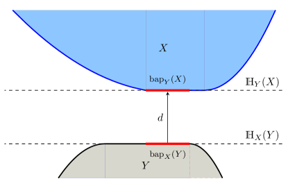
Figure 2: Disjoint convex sets $X$ and $Y$, BAPs and optimal hyperplanes.

Note that $\mathds{H}_{Y}(X)$ is well-defined since any points $\hat{x},\bar{x}\in\operatorname{bap}_{Y}(X)$ satisfy $\left\langle{\hat{x}-\bar{x}},{d}\right\rangle=0$. Definition 3.3 together with Fact 1(iii) imply that, for two disjoint closed convex sets $X,Y\subset\mathds{R}^{n}$ with attainable distance, $\operatorname{bap}_{Y}(X)=X\cap(Y+d)\subset\mathds{H}_{Y}(X)$ and $\operatorname{bap}_{X}(Y)=(X-d)\cap Y\subset\mathds{H}_{X}(Y)$. Figure 2 illustrates all these sets related to $X$ and $Y$ as well as the displacement vector $d$.

We now formally present the BAP error bound in a non-symmetrical version.

Definition 3.4 (Unilateral BAP error bound).

Let $X,Y\subset\mathds{R}^{n}$ be non-intersecting closed convex sets and assume that the distance between them is attained. We say that $X$ and $Y$ satisfy the unilateral BAP error bound (unilateral BAP-EB) at $x^{*}\in\operatorname{bap}_{Y}(X)$ if there exist a bound $\omega>0$ and a radius $\delta>0$ such that the following inequality holds

(6) $$\omega\operatorname{dist}(x,\operatorname{bap}_{Y}(X))\leq\operatorname{dist}(x,\mathds{H}_{Y}(X)),\text{ for all }x\in\mathscr{B}_{\delta}(x^{*})\cap X.$$

Definition 3.4 is a condition where the error bound is concentrated in only one of the two sets, therefore, the term unilateral. Nevertheless, the responsibility of carrying an error bound can be distributed between the sets $X$ and $Y$. In this regard, we will introduce in Definition 3.12 a more general error bound condition, in which a bilateral concern about the error bound is embedded.

Error bounds are, in general, regularity conditions that allow one to deal with non-isolated solutions; see, for example, [18, 19]. The BAP-EB resembles the well-known concept of local linear regularity[10, 12], formally presented in Definition 3.9. Linear regularity is also known as subtransversality [45]. BAP-EB requires, depending on the context, a further geometrical feature between the sets, in comparison to linear regularity. In Section 3.2, we present a detailed discussion on BAP-EB in which we compare it with the standard linear regularity (subtransversality) and with another regularity condition known as intrinsic transversality [39, 40].

Along this subsection, we are going to derive two important lemmas in which we consider the unilateral BAP-EB. They will be valuable tools towards establishing finite convergence of MAP in Section 4 under the more general error bound condition BAP-EB that we introduce later in Definition 3.12.

We present next a result encompassing a broader class of instances than the one in Lemma 3.1, since we are going to consider a closed convex set $X$ and a hyperplane $H$ with empty intersection and attainable distance. Here, the optimal supporting hyperplane $\mathds{H}_{H}(X)$ to $X$ regarding $H$ coincides precisely with $H+d$, that is, the hyperplane obtained by shifting $H$ by the displacement vector $d$. In this context, unilateral BAP-EB from Definition 3.4 is equivalent to local linear regularity. We prove this equivalence in Proposition 3.10. Taking this equivalence into account, the next result states that the standard linear regularity condition leads to finite convergence of alternating projections when the target convex sets are disjoint and one of them is a hyperplane.

Lemma 3.5 (Alternating projection step for a convex set versus hyperplane under inconsistency).

Let $X,H\subset\mathds{R}^{n}$ be a closed convex set and a hyperplane, respectively, and suppose that $X$ and $H$ are disjoint with attainable distance. Assume that $X$ and $H$ satisfy the unilateral BAP error bound Eq. 6 from Definition 3.4 at $x^{*}\in\operatorname{bap}_{H}(X)$, that is,

$$\omega\operatorname{dist}(x,\operatorname{bap}_{H}(X))\leq\operatorname{dist}(x,\mathds{H}_{H}(X)),\text{ for all }x\in\mathscr{B}_{\delta}(x^{*})\cap X,$$

with bound $\omega>0$ and radius $\delta>0$. By setting $r\coloneqq\min\left\{\omega\operatorname{dist}(X,H),\frac{\delta}{2}\right\}$, we have that

$$P_{X}P_{H}(z)\in\operatorname{bap}_{H}(X),\text{ for all }z\in\mathscr{B}_{r}(x^{*}).$$

Proof 3.6.

Take $z\in\mathscr{B}_{r}(x^{*})$, arbitrary, but fixed, with $x^{*}$ and $r$ as enunciated in the hypothesis. Set $\bar{z}\coloneqq P_{\operatorname{bap}_{H}(X)}(z)$ and $z_{H}\coloneqq P_{H}(z)$ and define

$$S\coloneqq\{s\in\mathds{R}^{n}\mid\left\langle{s-\bar{z}},{z_{H}-\bar{z}}\right\rangle\leq 0\}.$$

Since, $X\cap H=\emptyset$, we have that $z_{H}-\bar{z}\neq 0$ and thus, $S$ is an affine half-space. The keystone of the proof is to show that

$$X\subset S.$$

If this claim is proved, we get, directly from the characterization of a projection onto a closed convex set, that $\bar{z}=P_{X}(z_{H})=P_{X}P_{H}(z)$. Therefore, let us draw our attention to proving that 3.6 holds. Assume the contrary, that is, there exists a point $w\in X$ which does not lie in $S$. Then, for a sufficiently small $t\in(0,1]$, we have $x\coloneqq tw+(1-t)\bar{z}\in\mathscr{B}_{\delta}(x^{*})\cap X$. In fact, $x\in X$, by convexity. Now, we have that

(7) $$\left\lVert x-x^{*}\right\rVert =\left\lVert tw+(1-t)\bar{z}-x^{*}\right\rVert=\left\lVert t(w-x^{*})+(1-t)(\bar{z}-x^{*})\right\rVert$$

(8) $$\leq t\left\lVert w-x^{*}\right\rVert+(1-t)\left\lVert\bar{z}-x^{*}\right\rVert$$

(9) $$=t\left\lVert w-x^{*}\right\rVert+(1-t)\left\lVert P_{\operatorname{bap}_{H}(X)}(z)-P_{\operatorname{bap}_{H}(X)}(x^{*})\right\rVert$$

(10) $$\leq t\left\lVert w-x^{*}\right\rVert+(1-t)\left\lVert z-x^{*}\right\rVert$$

(11) $$<t\left\lVert w-x^{*}\right\rVert+(1-t)r$$

(12) $$\leq t\left\lVert w-x^{*}\right\rVert+(1-t)\frac{\delta}{2}$$

(13) $$<t\left\lVert w-x^{*}\right\rVert+\frac{\delta}{2},$$

where we used the definition of $x$, the convexity of the norm, the definition of $\bar{z}$ and the fact that $x^{*}\in\operatorname{bap}_{H}(X)$, the nonexpansiveness of the projection, the assumption $z\in\mathscr{B}_{r}(x^{*})$, the definition of $r$, and the fact that $1-t<1$, respectively. Let us take a fixed $t\in\left(0,\min\left\{1,\frac{\delta}{2\left\lVert w-x^{*}\right\rVert}\right\}\right]$. Thus, the correspondent $x=tw+(1-t)\bar{z}\in\mathscr{B}_{\delta}(x^{*})\cap X$. Note also that

(14) $$\left\langle{x-\bar{z}},{z_{H}-\bar{z}}\right\rangle =\left\langle{tw+(1-t)\bar{z}-\bar{z}},{z_{H}-\bar{z}}\right\rangle$$

(15) $$=t\left\langle{w-\bar{z}},{z_{H}-\bar{z}}\right\rangle$$

(16) $$>0,$$

since $t>0$ and $w\notin S$. Hence, $x\notin S$.

We proceed by showing that this point $x$ does not comply with the error bound condition Eq. 6, leading to a contradiction.

Simple Pythagoras arguments imply that $P_{\operatorname{bap}_{H}(X)}(z_{H})=\bar{z}\coloneqq P_{\operatorname{bap}_{H}(X)}(z)$, as we will see next. Let $z_{\mathds{H}}\coloneqq P_{\mathds{H}_{H}(X)}(z)$, where $\mathds{H}_{H}(X)$ is the optimal supporting hyperplane to $X$ regarding $H$ introduced in Definition 3.3. Reminding that, in this case, $\mathds{H}_{H}(X)=H+d$, we get $z_{\mathds{H}}=z_{H}+d$. Then,

(17) $$\left\lVert z-\bar{z}\right\rVert^{2}-\left\lVert\bar{z}-z_{\mathds{H}}\right\rVert^{2} =\left\lVert z-z_{\mathds{H}}\right\rVert^{2}=\left\lVert z-P_{\operatorname{bap}_{H}(X)}(z_{\mathds{H}})\right\rVert^{2}-\left\lVert P_{\operatorname{bap}_{H}(X)}(z_{\mathds{H}})-z_{\mathds{H}}\right\rVert^{2}$$

(18) $$\geq\left\lVert z-\bar{z}\right\rVert^{2}-\left\lVert P_{\operatorname{bap}_{H}(X)}(z_{\mathds{H}})-z_{\mathds{H}}\right\rVert^{2}.$$

Crossing out $\left\lVert P_{\operatorname{bap}_{H}(X)}(z_{\mathds{H}})-z_{\mathds{H}}\right\rVert^{2}$ yields $\left\lVert\bar{z}-z_{\mathds{H}}\right\rVert\leq\left\lVert P_{\operatorname{bap}_{H}(X)}(z_{\mathds{H}})-z_{\mathds{H}}\right\rVert$, which gives us $P_{\operatorname{bap}_{H}(X)}(z_{\mathds{H}})=\bar{z}$. Similarly, considering the Pythagoras relations, we have

(19) $$\left\lVert z_{H}-\bar{z}\right\rVert^{2}-\left\lVert\bar{z}-z_{\mathds{H}}\right\rVert^{2} =\left\lVert z_{H}-z_{\mathds{H}}\right\rVert^{2}=\left\lVert z_{H}-P_{\operatorname{bap}_{H}(X)}(z_{H})\right\rVert^{2}-\left\lVert P_{\operatorname{bap}_{H}(X)}(z_{H})-z_{\mathds{H}}\right\rVert^{2}$$

(20) $$\leq\left\lVert z_{H}-P_{\operatorname{bap}_{H}(X)}(z_{H})\right\rVert^{2}-\left\lVert\bar{z}-z_{\mathds{H}}\right\rVert^{2},$$

because $\left\lVert\bar{z}-z_{\mathds{H}}\right\rVert\leq\left\lVert P_{\operatorname{bap}_{H}(X)}(z_{H})-z_{\mathds{H}}\right\rVert$. After a cancellation, we get

$$\left\lVert z_{H}-\bar{z}\right\rVert\leq\left\lVert z_{H}-P_{\operatorname{bap}_{H}(X)}(z_{H})\right\rVert,$$

providing $P_{\operatorname{bap}_{H}(X)}(z_{H})=\bar{z}$.

The fact that $P_{\operatorname{bap}_{H}(X)}(z_{H})=\bar{z}$ implies that $\left\langle{s-\bar{z}},{z_{H}-\bar{z}}\right\rangle\leq 0,$ for all $s\in\operatorname{bap}_{H}(X)$, and we conclude by definition of $S$ that $\operatorname{bap}_{H}(X)\subset S$. On the other hand, recall that $\operatorname{bap}_{H}(X)\subset\mathds{H}_{H}(X)$ (see Definition 3.3). In particular,

$$\operatorname{bap}_{H}(X)\subset S\cap\mathds{H}_{H}(X).$$

Now, let us define $\hat{x}\coloneqq P_{S\cap\mathds{H}_{H}(X)}(x)$. Since $x\notin S$, we have $\left\langle{x-\bar{z}},{z_{H}-\bar{z}}\right\rangle>0$ and because $\hat{x}$ lies on the affine half-space $S$, it holds that $\left\langle{\hat{x}-\bar{z}},{z_{H}-\bar{z}}\right\rangle\leq 0$. Hence,

$$\left\langle{x-\hat{x}},{z_{H}-\bar{z}}\right\rangle=\left\langle{x-\bar{z}},{z_{H}-\bar{z}}\right\rangle+\left\langle{\bar{z}-\hat{x}},{z_{H}-\bar{z}}\right\rangle>0.$$

Moreover,

(21) $$0 <\left\langle{x-\hat{x}},{z_{H}-\bar{z}}\right\rangle=\left\langle{x-\hat{x}},{z_{H}-(\bar{z}-d)-d}\right\rangle$$

(22) $$=\left\langle{x-\hat{x}},{z_{H}-(\bar{z}-d)}\right\rangle-\left\langle{x-\hat{x}},{d}\right\rangle$$

(23) $$\leq\left\lVert x-\hat{x}\right\rVert\left\lVert z_{H}+d-\bar{z}\right\rVert-\left\langle{x-\hat{x}},{d}\right\rangle$$

(24) $$=\left\lVert x-\hat{x}\right\rVert\left\lVert P_{\mathds{H}_{H}(X)}(z)-P_{\mathds{H}_{H}(X)}(\bar{z})\right\rVert-\left\langle{x-\hat{x}},{d}\right\rangle$$

(25) $$\leq\left\lVert x-\hat{x}\right\rVert\left\lVert z-\bar{z}\right\rVert-\left\langle{x-\hat{x}},{d}\right\rangle$$

(26) $$<\left\lVert x-\hat{x}\right\rVert r-\left\langle{x-\hat{x}},{d}\right\rangle,$$

where the second inequality is by Cauchy-Schwarz, the third is by the nonexpansiveness of projection and the last one follows from $\left\lVert z-\bar{z}\right\rVert\leq\left\lVert z-x^{*}\right\rVert<r$. Therefore,

$$\left\langle{x-\hat{x}},{d}\right\rangle<r\left\lVert x-\hat{x}\right\rVert\leq\omega\left\lVert d\right\rVert\left\lVert x-\hat{x}\right\rVert,$$

by Eq. 26 and the definition of $r$.

Now, let $x_{H}\coloneqq P_{H}(x)$ and $x_{\mathds{H}}\coloneqq P_{\mathds{H}_{H}(X)}(x)=x_{H}+d$. Then,

$$\left\langle{x-\hat{x}},{d}\right\rangle=\left\langle{x-x_{\mathds{H}}+x_{\mathds{H}}-\hat{x}},{d}\right\rangle=\left\langle{x-x_{\mathds{H}}},{d}\right\rangle+\left\langle{x_{\mathds{H}}-\hat{x}},{d}\right\rangle=\left\langle{x-x_{\mathds{H}}},{d}\right\rangle,$$

as $\hat{x},x_{\mathds{H}}\in\mathds{H}_{H}(X)$ and $d\perp\mathds{H}_{H}(X)$. Due to the fact that $\mathds{H}_{H}(X)$ is a hyperplane, $x-x_{\mathds{H}}$ is collinear to $d$, so Cauchy-Schwarz holds sharply, that is, $\left\lvert\left\langle{x-x_{\mathds{H}}},{d}\right\rangle\right\rvert=\left\lVert x-x_{\mathds{H}}\right\rVert\left\lVert d\right\rVert$. Moreover, since $x\in X$, the inner product $\left\langle{x-x_{\mathds{H}}},{d}\right\rangle$ is nonnegative and thus $\left\langle{x-x_{\mathds{H}}},{d}\right\rangle=\left\lVert x-x_{\mathds{H}}\right\rVert\left\lVert d\right\rVert$, which combined with 3.6 and 3.6 provides

$$\left\lVert x-x_{\mathds{H}}\right\rVert\left\lVert d\right\rVert<\omega\left\lVert d\right\rVert\left\lVert x-\hat{x}\right\rVert.$$

This inequality, together with $\operatorname{bap}_{H}(X)\subset S\cap\mathds{H}_{H}(X)$, as proved in 3.6, yields

(27) $$\operatorname{dist}(x,\mathds{H}_{H}(X)) =\left\lVert x-x_{\mathds{H}}\right\rVert$$

(28) $$<\omega\left\lVert x-\hat{x}\right\rVert=\omega\operatorname{dist}(x,S\cap\mathds{H}_{H}(X))$$

(29) $$\leq\omega\operatorname{dist}(x,\operatorname{bap}_{H}(X)),$$

which contradicts the error bound assumption Lemma 3.5, because $x\in\mathscr{B}_{\delta}(x^{*})\cap X$ and $\operatorname{bap}_{H}(X)=X\cap\mathds{H}_{H}(X)$.

The previous result leads to another contribution of this paper. We show that the two ingredients, infeasibility and unilateral BAP-EB, imply that a single alternating projection step can locally reach a best approximation pair.

Lemma 3.7 (Alternating projection step under infeasibility and unilateral BAP-EB).

Let $X,Y\subset\mathds{R}^{n}$ be closed convex sets such that $X\cap Y=\emptyset$ and assume that the distance between them is attained. Assume that $X$ and $Y$ satisfy the unilateral BAP error bound Eq. 6 from Definition 3.4 at $x^{*}\in\operatorname{bap}_{Y}(X)$, that is,

$$\omega\operatorname{dist}(x,\operatorname{bap}_{Y}(X))\leq\operatorname{dist}(x,\mathds{H}_{Y}(X)),\text{ for all }x\in\mathscr{B}_{\delta}(x^{*})\cap X,$$

with bound $\omega>0$ and radius $\delta>0$. By setting $r\coloneqq\min\left\{\omega\operatorname{dist}(X,Y),\frac{\delta}{2}\right\}$ we have that for all $z\in\mathscr{B}_{r}(x^{*})$,

$$P_{X}P_{Y}(z)\in\operatorname{bap}_{Y}(X).$$

Proof 3.8.

Consider $x^{*}$ and $r$ as stated in the assumptions and let $z\in\mathscr{B}_{r}(x^{*})$ be arbitrary, but fixed. Now, set $z_{Y}\coloneqq P_{Y}(z)$ and $z^{\diamond}\coloneqq P_{\mathds{H}_{X}(Y)}(z_{Y})$, where $\mathds{H}_{X}(Y)$ is the optimal supporting hyperplane to $Y$ regarding $X$, i.e., $\mathds{H}_{Y}(X)=\mathds{H}_{X}(Y)+d$, where $d$ is the displacement vector. Moreover, using the nonexpansiveness of projection operators onto convex sets and that $x^{*}-d$ lies in both $Y$ and $\mathds{H}_{X}(Y)$, we obtain

(30) $$\left\lVert(z^{\diamond}+d)-x^{*}\right\rVert =\left\lVert z^{\diamond}-(x^{*}-d)\right\rVert$$

(31) $$=\left\lVert P_{\mathds{H}_{X}(Y)}(z_{Y})-P_{\mathds{H}_{X}(Y)}(x^{*}-d)\right\rVert$$

(32) $$\leq\left\lVert z_{Y}-(x^{*}-d)\right\rVert$$

(33) $$=\left\lVert P_{Y}(z)-P_{Y}(x^{*})\right\rVert$$

(34) $$\leq\left\lVert z-x^{*}\right\rVert\leq r,$$

that is, $z^{\diamond}+d\in\mathscr{B}_{r}(x^{*})$. Taking into account that $\operatorname{dist}(X,\mathds{H}_{X}(Y))=\operatorname{dist}(X,Y)=\left\lVert d\right\rVert$, Lemma 3.5 can be applied to $z^{\diamond}+d$, with $\mathds{H}_{X}(Y)$ playing the role of $H$, yielding $P_{X}P_{\mathds{H}_{X}(Y)}(z^{\diamond}+d)\in\operatorname{bap}_{\mathds{H}_{X}(Y)}(X)$. Note that $\operatorname{bap}_{\mathds{H}_{X}(Y)}(X)\subset X\cap\mathds{H}_{Y}(X)$ and clearly, the fact that the error bound constant $\omega$ in Lemma 3.7 is strictly positive implies that $\operatorname{bap}_{Y}(X)\cap\mathscr{B}_{r}(x^{*})=(X\cap\mathds{H}_{Y}(X))\cap\mathscr{B}_{r}(x^{*})$. Thus,

$$P_{X}(z^{\diamond})\in\operatorname{bap}_{Y}(X),$$

since $P_{X}(z^{\diamond})\in\mathscr{B}_{r}(x^{*})$. This occurs because $P_{X}(z^{\diamond})=P_{X}P_{\mathds{H}_{X}(Y)}(z^{\diamond}+d)$, $x^{*}\in X\cap\mathds{H}_{Y}(X)$, the nonexpansiveness of projections and Eq. 34 as

(35) $$\left\lVert P_{X}(z^{\diamond})-x^{*}\right\rVert =\left\lVert P_{X}P_{\mathds{H}_{X}(Y)}(z^{\diamond}+d)-P_{X}P_{\mathds{H}_{X}(Y)}(x^{*})\right\rVert$$

(36) $$\leq\left\lVert P_{\mathds{H}_{X}(Y)}(z^{\diamond}+d)-P_{\mathds{H}_{X}(Y)}(x^{*})\right\rVert$$

(37) $$\leq\left\lVert(z^{\diamond}+d)-x^{*}\right\rVert$$

(38) $$\leq r.$$

Bearing in mind the definition of $\mathds{H}_{X}(Y)$ and that $z_{Y}\in Y$, observe that there exists $t\leq 0$ such that $z_{Y}-z^{\diamond}=td$. For all $x\in X$, we have

(39) $$\left\langle{z_{Y}-P_{X}(z^{\diamond})},{x-P_{X}(z^{\diamond})}\right\rangle =\left\langle{z_{Y}-z^{\diamond}},{x-P_{X}(z^{\diamond})}\right\rangle+\left\langle{z^{\diamond}-P_{X}(z^{\diamond})},{x-P_{X}(z^{\diamond})}\right\rangle$$

(40) $$=\underbrace{t}_{\leq 0}\underbrace{\left\langle{d},{x-P_{X}(z^{\diamond})}\right\rangle}_{\geq 0}+\underbrace{\left\langle{z^{\diamond}-P_{X}(z^{\diamond})},{x-P_{X}(z^{\diamond})}\right\rangle}_{\leq 0}$$

(41) $$\leq 0,$$

where the second under-brace remark is by Fact 2 and the third is by characterization of the orthogonal projection of $z^{\diamond}$ onto $X$. Hence, Eq. 41 implies that $P_{X}(z_{Y})=P_{X}(z^{\diamond})$. Therefore, due to 3.8 and that $P_{X}P_{Y}(z)=P_{X}(z_{Y})$, it holds that

$$P_{X}P_{Y}(z)\in\operatorname{bap}_{Y}(X),$$

proving the theorem.

3.2 BAP-EB and other regularity conditions

We now proceed to discuss the connection of BAP-EB with two other regularity conditions: local linear regularity, which is the keystone for providing linear convergence of MAP [10, Corollary 3.14], and intrinsic transversality.

First, we show that unilateral BAP-EB implies the standard local linear regularity and moreover, both coincide in the context of Lemma 3.5, that is, when one of the sets is a hyperplane. This is proved in Proposition 3.10 below. This subsection ends with a proof that BAP-EB is more general than intrinsic transversality. For clarity, we present the definitions of linear regularity and intrinsic transversality.

Definition 3.9 (Local linear regularity [10, Definition 3.11]).

Let $X,Y\subset\mathds{R}^{n}$ be closed convex sets such that $X\cap Y=\emptyset$, assume that the distance between them is attained and suppose that $d$ is the displacement vector. We say that $X$ and $Y$ are locally linearly regular if for some point $x^{*}\in\operatorname{bap}_{Y}(X)$ there exist a bound $\kappa>0$ and a radius $\rho>0$ and such that, for all $z\in\mathscr{B}_{\rho}(x^{*})$,

$$\operatorname{dist}(z,\operatorname{bap}_{Y}(X))\leq\kappa\max\{\operatorname{dist}(z,X),\operatorname{dist}(z,Y+d)\}.$$

Proposition 3.10.

Let $X,Y\subset\mathds{R}^{n}$ be closed convex sets, suppose that $X$ and $Y$ are disjoint with attainable distance and let $d$ be the displacement vector. Then, the unilateral BAP-EB condition from Definition 3.4 implies local linear regularity. If, in addition, $Y$ is a hyperplane, then local linear regularity is equivalent to the unilateral BAP-EB.

Proof 3.11.

Assume that the unilateral BAP error bound condition from Definition 3.4 holds, that is, for some point $x^{*}\in\operatorname{bap}_{Y}(X)$ there exist $\omega>0$ and $\delta>0$ such that, for all $x\in\mathscr{B}_{\delta}(x^{*})\cap X$,

$$\omega\operatorname{dist}(x,\operatorname{bap}_{Y}(X))\leq\operatorname{dist}(x,\mathds{H}_{Y}(X)).$$

Note that, for all $x\in X$, we have $\operatorname{dist}(x,\mathds{H}_{Y}(X))\leq\operatorname{dist}(x,Y+d)$. From the fact that $\operatorname{bap}_{Y}(X)=X\cap(Y+d)$, it follows that

$$\operatorname{dist}(x,X\cap(Y+d))\leq\frac{1}{\omega}\operatorname{dist}(x,Y+d),$$

for all $x\in\mathscr{B}_{\delta}(x^{*})\cap X$. Using [10, Lemma 4.1] in the last inequality, with $X$ playing the role of $M$ and $Y+d$ playing the role of $N$, we get

$$\operatorname{dist}(z,X\cap(Y+d))\leq\left(\frac{2}{\omega}+1\right)\max\{\operatorname{dist}(z,X),\operatorname{dist}(z,Y+d)\},$$

for all $z\in\mathscr{B}_{\frac{\delta}{2}}(x^{*})$. Thus, the local linear regularity holds with $\kappa\coloneqq\frac{2}{\omega}+1$ and $\rho\coloneqq\frac{\delta}{2}$.

To complete the proof, we just have to show that, if $Y$ is a hyperplane, local linear regularity implies Eq. 6, as in this case $Y+d$ coincides with $\mathds{H}_{Y}(X)$, the optimal supporting hyperplane to $X$ regarding $Y$. Therefore, for all points $z\in X$, $\max\{\operatorname{dist}(z,X),\operatorname{dist}(z,Y+d)\}=\operatorname{dist}(z,Y+d)=\operatorname{dist}(z,\mathds{H}_{Y}(X))$. Hence, the result follows, with $\omega\coloneqq\frac{1}{\kappa}$ and $\delta\coloneqq\rho$.

Later, in Example 5.2, we will see that if none of the sets is a hyperplane, local linear regularity might not coincide with the unilateral BAP error bound from Definition 3.4.

Next, we introduce a bilateral error bound condition (referred to as BAP-EB), which is more general than the unilateral BAP-EB from Definition 3.4 and also implies finite convergence of MAP under inconsistency; see Theorem 4.9. Furthermore, we will see in Theorem 4.11 that, under inconsistency, a given MAP sequence converges in a finite number of steps if, and only if, the BAP-EB is satisfied along it.

Definition 3.12 (BAP error bound).

Let $X,Y\subset\mathds{R}^{n}$ be non-intersecting closed convex sets and assume that the distance between them is attained. We say that $X$ and $Y$ satisfy the BAP error bound (BAP-EB) at $x^{*}\in\operatorname{bap}_{Y}(X)$ if there exist a bound $\omega>0$ and a radius $\delta>0$ such that, for all $x\in\mathscr{B}_{\delta}(x^{*})\cap X$, at least one of the following inequalities holds

$$\omega\operatorname{dist}(P_{Y}(x),\operatorname{bap}_{X}(Y)) \leq\operatorname{dist}(P_{Y}(x),\mathds{H}_{X}(Y)),$$

$$\omega\operatorname{dist}(P_{X}P_{Y}(x),\operatorname{bap}_{Y}(X)) \leq\operatorname{dist}(P_{X}P_{Y}(x),\mathds{H}_{Y}(X)).$$

Before starting to state theorems on finite convergence of MAP and variants, we will compare BAP-EB with intrinsic transversality. Drusvyatskiy presents intrinsic transversality in [39, Definition 3.1] and comments on its importance. The definition originally considers intersecting sets, and says that two closed sets $X,Y\subset\mathds{R}^{n}$ are intrinsically transversal at a common point if there exists an angle $\alpha\in\left(0,\frac{\pi}{2}\right]$ such that, near this common point, any two points $x\in X\backslash Y$ and $y\in Y\backslash X$ cannot have difference $x-y$ simultaneously making an angle strictly less than $\alpha$ with both the normal cones $-\mathscr{N}_{X}(x)$ and $\mathscr{N}_{Y}(y)$.

The concept of intrinsic transversality was adapted for nonintersecting sets in [23]. This nice manuscript first appeared in the form of a preprint on arXiv a few days after the submission of the present paper. The authors of [23] have similar results to ours as they derived finite convergence of MAP under inconsistency and intrinsic transversality. We will actually prove that intrinsic transversality for nonintersecting convex sets implies BAP-EB. However, the converse is not true. Example 5.3 shows that BAP-EB is more general. More than that, BAP-EB along a MAP sequence is a necessary and sufficient condition for its finite convergence under infeasibility; see Theorem 4.11. Next, we provide the definition of intrinsic transversality for two nonintersecting closed convex sets introduced in [23, Condition 1’].

Definition 3.13 (Intrinsic transversality for disjoint sets).

Two closed convex sets $X,Y\subset\mathds{R}^{n}$ with empty intersection and attainable distance are intrinsically transversal at $(x^{*},y^{*})\in\operatorname{bap}(X,Y)$ if there exist $\kappa\in(0,1)$ and $\delta>0$ such that

$$\max\left\{\operatorname{dist}\left(\frac{x-y}{\left\lVert x-y\right\rVert},\mathscr{N}_{Y}(y)\right),\operatorname{dist}\left(\frac{x-y}{\left\lVert x-y\right\rVert},-\mathscr{N}_{X}(x)\right)\right\}\geq\kappa,$$

for all $x\in X\cap\mathscr{B}_{\delta}(x^{*})$ and $y\in\big{(}Y\backslash\operatorname{bap}_{X}(Y)\big{)}\cap\mathscr{B}_{\delta}(y^{*})$.

We point out that the previous definition is not symmetrical. It is unilateral, since one is considering local points $y\in Y$ such that $\operatorname{dist}(X,y)>\operatorname{dist}(X,Y)$, but this condition is not required for points in $X$.

We now establish that intrinsic transversality is a sufficient condition for BAP-EB to be fulfilled.

Proposition 3.14 (Intrinsic transversality implies BAP-EB).

If intrinsic transversality from Definition 3.13 is satisfied, then BAP-EB from Definition 3.12 holds.

Proof 3.15.

We are going to prove the statement by showing that the absence of BAP-EB prevents intrinsic transversality to hold.

Consider two closed and convex sets $X,Y\in\mathds{R}^{n}$ with empty intersection and attainable distance. Let $(x^{*},y^{*})\in\operatorname{bap}(X,Y)$ and suppose that BAP-EB does not hold at $x^{*}$. The lack of BAP-EB guarantees the existence of a sequence $(x^{k})_{k\in\mathds{N}}\subset X$ converging to $x^{*}$ such that the sequence defined by $y^{k}\coloneqq P_{Y}(x^{k})$ has no term in $\operatorname{bap}_{X}(Y)$ and converges to $y^{*}$, and the sequence determined by $w^{k}\coloneqq P_{X}P_{Y}(x^{k})$ does not have any term in $\operatorname{bap}_{Y}(X)$ and converges to $x^{*}$. The existence of such sequence $(x^{k})_{k\in\mathds{N}}$ is indeed easy to verify when denying both inequalities Definition 3.12 in BAP-EB.

Obviously, $x^{k}-y^{k}\in\mathscr{N}_{Y}(y^{k})$ and $w^{k}-y^{k}\in-\mathscr{N}_{X}(w^{k})$. Taking into account the nonexpansiveness of projections, we have $x^{k}-y^{k}\to x^{*}-y^{*}$ and $w^{k}-y^{k}\to x^{*}-y^{*}$.

Hence,

(42) $$\lim_{k\to\infty}\operatorname{dist}\left(\frac{w^{k}-y^{k}}{\left\lVert w^{k}-y^{k}\right\rVert},\mathscr{N}_{Y}(y^{k})\right) \leq\lim_{k\to\infty}\left\lVert\frac{w^{k}-y^{k}}{\left\lVert w^{k}-y^{k}\right\rVert}-\frac{x^{k}-y^{k}}{\left\lVert x^{k}-y^{k}\right\rVert}\right\rVert$$

(43) $$=\left\lVert\frac{x^{*}-y^{*}}{\left\lVert x^{*}-y^{*}\right\rVert}-\frac{x^{*}-y^{*}}{\left\lVert x^{*}-y^{*}\right\rVert}\right\rVert=0,$$

and

(44) $$\lim_{k\to\infty}\operatorname{dist}\left(\frac{w^{k}-y^{k}}{\left\lVert w^{k}-y^{k}\right\rVert},-\mathscr{N}_{X}(w^{k})\right) \leq\lim_{k\to\infty}\left\lVert\frac{w^{k}-y^{k}}{\left\lVert w^{k}-y^{k}\right\rVert}-\frac{w^{k}-y^{k}}{\left\lVert w^{k}-y^{k}\right\rVert}\right\rVert=0,$$

which invalids Definition 3.13, i.e., intrinsic transversality fails.

4 Finite convergence of projection-based methods

4.1 Finite convergence of MAP

In this subsection we present straightforward consequences of Lemmas 3.1, 3.5, and 3.7 on MAP. The first theorem establishes finite convergence of MAP for a polyhedron and a disjoint hyperplane. We then show that under local linear regularity, MAP for a closed convex set and a disjoint hyperplane also converges in a finite number of steps, as for a hyperplane versus a closed convex set, local linear regularity coincides with BAP-EB; recall Proposition 3.10. Then, we see in Theorem 4.5 that infeasibility combined with unilateral BAP-EB implies finite convergence of alternating projections for two closed convex sets. Finally, in Theorem 4.9, we prove the most important result of this work, namely, that BAP-EB from Definition 3.12 under inconsistency also yields finite convergence of MAP.

Theorem 4.1 (Finite convergence of MAP for polyhedron versus hyperplane under inconsistency).

Consider two nonempty sets $\Omega,H\subset\mathds{R}^{n}$ such that $\Omega$ is a polyhedron, $H$ is a hyperplane and $\Omega\cap H=\emptyset$. Let $x^{0}\in\mathds{R}^{n}$ be given and $(x^{k})_{k\in\mathds{N}}$ be the MAP sequence defined by $x^{k+1}\coloneqq P_{\Omega}P_{H}(x^{k})$. Then, $(x^{k})_{k\in\mathds{N}}$ converges in finitely many steps to $\bar{x}\in\operatorname{bap}_{H}(\Omega)$.

Proof 4.2.

Fact 7 provides that $\operatorname{dist}(\Omega,H)$ is attained, as $H$ is also a polyhedron. Hence, the sequence $(x^{k})_{k\in\mathds{N}}$ converges to some $\bar{x}\in\operatorname{bap}_{H}(\Omega)$ (Fact 3(i)). Hence, for a sufficiently large $\bar{k}$, $\operatorname{dist}(x^{\bar{k}},\operatorname{bap}_{H}(\Omega))\leq r$, where $r$ set as in Lemma 3.1. Therefore, by Lemma 3.1, $x^{\bar{k}+1}=P_{\Omega}P_{H}(x^{\bar{k}})=\bar{x}$, hence proved.

Theorem 4.1 alone encompasses a very relevant setting featuring non-isolated solutions as it concerns a hyperplane versus a polyhedron (see Example 5.1 for an application on linear programming). Below, we will state results for non-intersecting convex sets under BAP-EB conditions beyond the polyhedral-affine setting.

Theorem 4.3 (Finite convergence of MAP for a convex set versus hyperplane under inconsistency).

Let $X,H\subset\mathds{R}^{n}$ be a closed convex set and a hyperplane, respectively, and suppose that $X$ and $H$ are disjoint with attainable distance. Assume that $X$ and $H$ satisfy the BAP error bound Eq. 6 from Definition 3.4 at $x^{*}\in\operatorname{bap}_{H}(X)$ with bounds $\omega>0$ and radius $\delta>0$. By setting $r\coloneqq\min\left\{\omega\operatorname{dist}(X,H),\frac{\delta}{2}\right\}$, we have that for any given $x^{0}\in\mathds{R}^{n}$, the MAP sequence $(x^{k})_{k\in\mathds{N}}$ defined by $x^{k+1}\coloneqq P_{X}P_{H}(x^{k})$ converges to a point $\bar{x}\in\operatorname{bap}_{H}(X)$. Moreover, if there exists an index $\bar{k}\geq 0$, such that $x^{\bar{k}}\in\mathscr{B}_{r}(x^{*})$, then $x^{\bar{k}+1}=\bar{x}$, that is, in this case, MAP converges in at most $\bar{k}+1$ steps.

Proof 4.4.

It is well-known that MAP converges globally for two closed convex sets with attainable distance (see Fact 3(i)) and thus, the first part of item (ii) follows. Its second part is a straightforward consequence of Lemma 3.5.

Theorem 4.5 (Finite convergence of MAP under infeasibility and unilateral BAP-EB).

Let $X,Y\subset\mathds{R}^{n}$ be closed convex sets such that $X\cap Y=\emptyset$ and assume that the distance between them is attained. Assume that $X$ and $Y$ satisfy the unilateral BAP error bound of Definition 3.4 at $x^{*}\in\operatorname{bap}_{Y}(X)$ with bound $\omega>0$ and radius $\delta>0$. Set $r\coloneqq\min\left\{\omega\operatorname{dist}(X,Y),\frac{\delta}{2}\right\}$, and then we have that for any given $x^{0}\in\mathds{R}^{n}$, the MAP sequence $(x^{k})_{k\in\mathds{N}}$ defined by $x^{k+1}\coloneqq P_{X}P_{Y}(x^{k})$ converges to a point $\bar{x}\in\operatorname{bap}_{Y}(X)$. Moreover, if there exists an index $\bar{k}\geq 0$, such that $x^{\bar{k}}\in\mathscr{B}_{r}(x^{*})$, then $x^{\bar{k}+1}=\bar{x}$, that is, in this case, MAP converges in at most $\bar{k}+1$ steps.

Proof 4.6.

The result follows directly from Fact 3(i) and Lemma 3.7.

In order to prove finite convergence of MAP under the bilateral BAP-EB from Definition 3.12, we need the following auxiliary proposition.

Proposition 4.7.

Let $X,Y\subset\mathds{R}^{n}$ be closed convex sets such that $X\cap Y=\emptyset$, assume that the distance between them is attained. Consider a sequence $(z^{k})_{k\in\mathds{N}}\subset X$ converging to a point $z^{*}\in\operatorname{bap}_{Y}(X)$. Assume there exists $\omega>0$ such that, for all $k$,

$$\omega\operatorname{dist}(z^{k},\operatorname{bap}_{Y}(X))\leq\operatorname{dist}(z^{k},\mathds{H}_{Y}(X)).$$

Then,

$$\omega\operatorname{dist}(z,\operatorname{bap}_{Y}(X))\leq\operatorname{dist}(z,\mathds{H}_{Y}(X))$$

holds for all $z\in\overline{S}\coloneqq\operatorname{cl}\left(\operatorname{conv}\left((z^{k})_{k\in\mathds{N}}\cup\operatorname{bap}_{Y}(X)\right)\right)$. Moreover, $\operatorname{dist}(\overline{S},Y)=\operatorname{dist}(X,Y)$, $\operatorname{bap}_{Y}(\overline{S})=\operatorname{bap}_{Y}(X)$ and $\mathds{H}_{Y}(\overline{S})=\mathds{H}_{Y}(X)$.

Proof 4.8.

We start proving that the convex hull $S\coloneqq\operatorname{conv}\left((z^{k})_{k\in\mathds{N}}\cup\operatorname{bap}_{Y}(X)\right)$ satisfies the announced error bound Proposition 4.7. This will be done by induction over the sets

$$S_{k}\coloneqq\operatorname{conv}\left(\left\{z^{0},z^{1},\ldots,z^{k}\right\}\cup\operatorname{bap}_{Y}(X)\right).$$

Note that $S_{0}=\{z_{\lambda}\in X\mid z_{\lambda}=\lambda z^{0}+(1-\lambda)v,\;\lambda\in[0,1],v\in\operatorname{bap}_{Y}(X)\}$. Taking arbitrary but fixed $v\in\operatorname{bap}_{Y}(X)$ and $\lambda\in[0,1]$, we define accordingly $z_{\lambda}\in S_{0}$ and denote by $\bar{z}_{\lambda}\coloneqq P_{\operatorname{bap}_{Y}(X)}(z_{\lambda})$and by $\bar{z}^{0}\coloneqq P_{\operatorname{bap}_{Y}(X)}(z^{0})$. Note that $\hat{z}_{\lambda}\coloneqq\lambda\bar{z}^{0}+(1-\lambda)v\in\operatorname{bap}_{Y}(X)$, so we get

(45) $$\omega\operatorname{dist}(z_{\lambda},\operatorname{bap}_{Y}(X)) =\omega\left\lVert z_{\lambda}-\bar{z}_{\lambda}\right\rVert$$

(46) $$\leq\omega\left\lVert z_{\lambda}-\hat{z}_{\lambda}\right\rVert$$

(47) $$=\omega\left\lVert\lambda z^{0}+(1-\lambda)v-(\lambda\bar{z}^{0}+(1-\lambda)v)\right\rVert$$

(48) $$=\omega\left\lVert\lambda(z^{0}-\bar{z}^{0})\right\rVert$$

(49) $$=\lambda\omega\operatorname{dist}\left(z^{0},\operatorname{bap}_{Y}(X)\right).$$

Define now $\tilde{z}_{\lambda}\coloneqq P_{\mathds{H}_{Y}(X)}(z_{\lambda})$. Since $\mathds{H}_{Y}(X)$ is a hyperplane we get

$$\tilde{z}_{\lambda}=P_{\mathds{H}_{Y}(X)}(\lambda z^{0}+(1-\lambda)v)=\lambda P_{\mathds{H}_{Y}(X)}(z^{0})+(1-\lambda)P_{\mathds{H}_{Y}(X)}(v)=\lambda\tilde{z}^{0}+(1-\lambda)v,$$

using in the last equality that $\tilde{z}^{0}\coloneqq P_{\mathds{H}_{Y}(X)}(z^{0})$ and $v\in\operatorname{bap}_{Y}(X)\subset\mathds{H}_{Y}(X)$. Then,

(50) $$\operatorname{dist}(z_{\lambda},\mathds{H}_{Y}(X)) =\left\lVert z_{\lambda}-\tilde{z}_{\lambda}\right\rVert$$

(51) $$=\left\lVert(\lambda z^{0}+(1-\lambda)v)-(\lambda\tilde{z}^{0}+(1-\lambda)v)\right\rVert$$

(52) $$=\left\lVert\lambda(z^{0}-\tilde{z}^{0})\right\rVert$$

(53) $$=\lambda\operatorname{dist}\left(z^{0},\mathds{H}_{Y}(X)\right)).$$

The hypothesis Proposition 4.7 for $k=0$ reads as

$$\omega\operatorname{dist}\left(z^{0},\operatorname{bap}_{Y}(X)\right)\leq\operatorname{dist}\left(z^{0},\mathds{H}_{Y}(X)\right).$$

Multiplying this inequality by $\lambda\in[0,1]$ and combining it with equalities Eqs. 49 and 53, gives us the first step of the induction.

Now, note that

$$S_{k+1}=\operatorname{conv}\left(\left\{z^{0},z^{1},\ldots,z^{k},z^{k+1}\right\}\cup\operatorname{bap}_{Y}(X)\right)=\operatorname{conv}(S_{k}\cup\{z^{k+1}\}),$$

our induction hypothesis says that all $u\in S_{k}$ satisfies

$$\omega\operatorname{dist}\left(u,\operatorname{bap}_{Y}(X)\right)\leq\operatorname{dist}\left(u,\mathds{H}_{Y}(X)\right)$$

and inequality Proposition 4.7 specialized for $k+1$ gives us

$$\omega\operatorname{dist}\left(z^{k+1},\operatorname{bap}_{Y}(X)\right)\leq\operatorname{dist}\left(z^{k+1},\mathds{H}_{Y}(X)\right).$$

Consider an arbitrary point in $S_{k+1}$. It can be written as $z_{\lambda}=\lambda u+(1-\lambda)z^{k+1}$, for some $u\in S_{k}$ and $\lambda\in[0,1]$. Let $\bar{u},\bar{z}^{k+1}$ be the distance realizers of $u,z^{k+1}$ with respect to $\operatorname{bap}_{Y}(X)$, respectively and $\tilde{u},\tilde{z}^{k+1}$ be the distance realizers of $u,z^{k+1}$ regarding $\mathds{H}_{Y}(X)$, respectively. Note that $\tilde{z}_{\lambda}\coloneqq P_{\mathds{H}_{Y}(X)}(z_{\lambda})=\lambda\tilde{u}+(1-\lambda)\tilde{z}^{k+1}$, since $\mathds{H}_{Y}(X)$ is a hyperplane. Moreover, by the same token, $u-\tilde{u}=\alpha d$ and $z^{k+1}-\tilde{z}^{k+1}=\beta d$, for some $\alpha,\beta\geq 0$ and where $d$ is the displacement vector (pointing from $Y$ to $X$). Thus,

(54) $$\operatorname{dist}\left(z_{\lambda},\mathds{H}_{Y}(X)\right) =\left\lVert z_{\lambda}-\tilde{z}_{\lambda}\right\rVert=\left\lVert\lambda(u-\tilde{u})+(1-\lambda)(z^{k+1}-\tilde{z}^{k+1})\right\rVert$$

(55) $$=\left\lVert\lambda(\alpha d)+(1-\lambda)(\beta d)\right\rVert=\left\lVert(\lambda\alpha+(1-\lambda)\beta)d\right\rVert$$

(56) $$=(\lambda\alpha+(1-\lambda)\beta)\left\lVert d\right\rVert=\lambda\alpha\left\lVert d\right\rVert+(1-\lambda)\beta\left\lVert d\right\rVert$$

(57) $$=\lambda\left\lVert\alpha d\right\rVert+(1-\lambda)\left\lVert\beta d\right\rVert=\lambda\left\lVert u-\tilde{u}\right\rVert+(1-\lambda)\left\lVert z^{k+1}-\tilde{z}^{k+1}\right\rVert$$

(58) $$=\lambda\operatorname{dist}\left(u,\mathds{H}_{Y}(X)\right)+(1-\lambda)\operatorname{dist}\left(z^{k+1},\mathds{H}_{Y}(X)\right).$$

Now, the point $\hat{z}_{\lambda}\coloneqq\lambda\bar{u}+(1-\lambda)\bar{z}^{k+1}$ belongs to $\operatorname{bap}_{Y}(X)$ but need not coincide with $\bar{z}_{\lambda}$, the distance realizer of $z_{\lambda}$ to $\operatorname{bap}_{Y}(X)$. Nevertheless, we can write

(59) $$\omega\operatorname{dist}(z_{\lambda},\operatorname{bap}_{Y}(X)) =\omega\left\lVert z_{\lambda}-\bar{z}_{\lambda}\right\rVert\leq\omega\left\lVert z_{\lambda}-\hat{z}_{\lambda}\right\rVert$$

(60) $$=\omega\left\lVert(\lambda u+(1-\lambda)z^{k+1})-(\lambda\bar{u}+(1-\lambda)\bar{z}^{k+1})\right\rVert$$

(61) $$\leq\lambda\omega\left\lVert u-\bar{u}\right\rVert+(1-\lambda)\omega\left\lVert z^{k+1}-\bar{z}^{k+1}\right\rVert$$

(62) $$=\lambda\omega\operatorname{dist}\left(u,\operatorname{bap}_{Y}(X)\right)+(1-\lambda)\omega\operatorname{dist}\left(z^{k+1},\operatorname{bap}_{Y}(X)\right)$$

(63) $$\leq\lambda\operatorname{dist}\left(u,\mathds{H}_{Y}(X)\right)+(1-\lambda)\operatorname{dist}\left(z^{k+1},\mathds{H}_{Y}(X)\right)$$

(64) $$=\operatorname{dist}\left(z_{\lambda},\mathds{H}_{Y}(X)\right),$$

where the last inequality is by 4.8 and 4.8 and the last equality is due to Eq. 58. Therefore, the induction argument is completed and the error bound Proposition 4.7 holds for all points in $S$.

Next we are going to prove that the error bound Proposition 4.7 extends to $\overline{S}$, the closure of $S$. Take $s\in\overline{S}$. Then, there exists a sequence $(s^{\ell})_{\ell\in\mathds{N}}\subset S$ so that $s^{\ell}\to s$. Note that we have just proven the error bound for all points in $S$, thus all $s^{\ell}$ satisfies

$$\omega\operatorname{dist}(s^{\ell},\operatorname{bap}_{Y}(X))\leq\operatorname{dist}(s^{\ell},\mathds{H}_{Y}(X)).$$

Taking into account that the distance functions to both sets $\operatorname{bap}_{Y}(X)$ and $\mathds{H}_{Y}(X)$ are continuous, we can take limits as $\ell$ goes to infinity in both sides of the previous inequality, getting the result.

Finally, since $\operatorname{bap}_{Y}(X)\subset\overline{S}\subset X$, we have $\operatorname{dist}(X,Y)\leq\operatorname{dist}(\overline{S},Y)\leq\operatorname{dist}(\operatorname{bap}_{Y}(X),Y)=\operatorname{dist}(X,Y)$, that is, $\operatorname{dist}(\overline{S},Y)=\operatorname{dist}(X,Y)$. Thus, $\operatorname{bap}_{Y}(\overline{S})=\operatorname{bap}_{Y}(X)$ and $\mathds{H}_{Y}(\overline{S})=\mathds{H}_{Y}(X)$

We are now ready to establish finite convergence of MAP under inconsistency added by BAP-EB.

Theorem 4.9 (Finite convergence of MAP under infeasibility and BAP-EB).

Let $X,Y\subset\mathds{R}^{n}$ be closed convex sets such that $X\cap Y=\emptyset$, assume that the distance between them is attained and let $x^{0}\in\mathds{R}^{n}$ be given. Then, the MAP sequence $(x^{k})_{k\in\mathds{N}}$, defined by $x^{k+1}\coloneqq P_{X}P_{Y}(x^{k})$, converges to some $x^{*}\in\operatorname{bap}_{Y}(X)$. If BAP-EB from Definition 3.12 is satisfied by $X$ and $Y$ at $x^{*}$, then $(x^{k})_{k\in\mathds{N}}$ converges to $x^{*}$ in a finite number of steps.

Proof 4.10.

The convergence of the MAP sequence to some $x^{*}\in\operatorname{bap}_{Y}(X)$ for two disjoint closed convex sets $X$ and $Y$, assuming its distance is attainable, is due to Fact 3(i). Assume BAP-EB as in the statement of the theorem and that the MAP sequence $(x^{k})_{k\in\mathds{N}}$ does not converge in a finite number of steps. Thus, since MAP iterates satisfy $\left\lVert x^{k+1}-x^{*}\right\rVert\leq\left\lVert x^{k}-x^{*}\right\rVert$, all the terms $x^{k}$ lie outside $\operatorname{bap}_{Y}(X)$ and, in particular, they are all different from $x^{*}$.

Note that BAP-EB consists of all points $x\in X$ near $x^{*}$ fulfilling at least one of the two inequalities Definition 3.12 given in Definition 3.12. In the following we divide our proof in two cases.

First, let us assume that there is a subsequence of the MAP sequence satisfying the second inequality in Definition 3.12. So, we have an infinite set of indexes $J\subset\mathds{N}$, such that

$$\omega\operatorname{dist}(P_{X}P_{Y}(x^{k-1}),\operatorname{bap}_{Y}(X))\leq\operatorname{dist}(P_{X}P_{Y}(x^{k-1}),\mathds{H}_{Y}(X)),\text{ for all }k\in J,$$

which is the same as

$$\omega\operatorname{dist}(x^{k},\operatorname{bap}_{Y}(X))\leq\operatorname{dist}(x^{k},\mathds{H}_{Y}(X)),\text{ for all }k\in J.$$

Let us define the closed convex set $\overline{S}\coloneqq\operatorname{cl}\left(\operatorname{conv}\left((x^{k})_{k\in J}\cup\operatorname{bap}_{Y}(X)\right)\right)\subset X$. Clearly, $x^{*}\in\overline{S}$ and, since 4.10 holds and $(x^{k})_{k\in J}$ converges to $x^{*}$, Proposition 4.7 can be used. Then, for all $z\in\overline{S}$,

$$\omega\operatorname{dist}(z,\operatorname{bap}_{Y}(\overline{S}))=\omega\operatorname{dist}(z,\operatorname{bap}_{Y}(X))\leq\operatorname{dist}(z,\mathds{H}_{Y}(X))=\operatorname{dist}(z,\mathds{H}_{Y}(\overline{S})).$$

This inequality means that the unilateral BAP-EB condition from Definition 3.4 is satisfied for $\overline{S}$ and $Y$ at $x^{*}$. Therefore, Lemma 3.7 applies because, for all $k\in\mathds{N}$ sufficiently large, $x^{k-1}$ is near enough to $x^{*}$. Hence, for all large $k$, we have $P_{\overline{S}}P_{Y}(x^{k-1})\in\operatorname{bap}_{Y}(\overline{S})=\operatorname{bap}_{Y}(X)$, where the equality of the BAP sets follows from Proposition 4.7.

Recall that, for all $k\in J$, $x^{k}$ belongs to $\overline{S}\subset X$. Moreover, for each $k\in J$ there exists $j_{k}\in\mathds{N}$ such that $k+j_{k}\in J$ and thus $x^{k+j_{k}}\in\overline{S}$, and, in addition, $\left\lVert x^{k+j_{k}}-x^{*}\right\rVert\leq\left\lVert x^{k}-x^{*}\right\rVert$.

Note that $x^{k+j_{k}}=P_{X}P_{Y}(x^{k+j_{k}-1})$ and that $P_{Y}(x^{k+j_{k}-1})$ approaches $P_{Y}(x^{*})$, when $k$ goes to infinity. Thus, for all large $k\in J$, $P_{\overline{S}}P_{Y}(x^{k+j_{k}-1})\in\operatorname{bap}_{Y}(X)$. Then, by the characterization of projection onto convex sets, we get

(65) $$\left\langle{P_{Y}(x^{k+j_{k}-1})-P_{\overline{S}}P_{Y}(x^{k+j_{k}-1})},{x^{k+j_{k}}-P_{\overline{S}}P_{Y}(x^{k+j_{k}-1})}\right\rangle\leq 0.$$

Note that both vectors in the above inner product are different from zero, because $P_{\overline{S}}P_{Y}(x^{k+j_{k}-1})$ is in $\operatorname{bap}_{Y}(X)$ but not in $Y$ and $x^{k+j_{k}}$ is in $\overline{S}$ but not in $\operatorname{bap}_{Y}(X)$. Then,

$$\left\lVert P_{Y}(x^{k+j_{k}-1})-x^{k+j_{k}}\right\rVert>\left\lVert P_{Y}(x^{k+j_{k}-1})-P_{\overline{S}}P_{Y}(x^{k+j_{k}-1})\right\rVert.$$

On the other hand, since $\overline{S}\subset X$, we have

(66) $$\left\lVert P_{Y}(x^{k+j_{k}-1})-P_{\overline{S}}P_{Y}(x^{k+j_{k}-1})\right\rVert\geq \left\lVert P_{Y}(x^{k+j_{k}-1})-P_{X}P_{Y}(x^{k+j_{k}-1})\right\rVert$$

(67) $$= \left\lVert P_{Y}(x^{k+j_{k}-1})-x^{k+j_{k}}\right\rVert$$

(68) $$> \left\lVert P_{Y}(x^{k+j_{k}-1})-P_{\overline{S}}P_{Y}(x^{k+j_{k}-1})\right\rVert,$$

which is a contradiction.

For second case, suppose now that there exists a subsequence $(x^{k})_{k\in J^{\prime}}$ of the MAP sequence $(x^{k})_{k\in\mathds{N}}$ satisfying the first inequality in Definition 3.12, that is,

$$\omega\operatorname{dist}(P_{Y}(x^{k}),\operatorname{bap}_{X}(Y))\leq\operatorname{dist}(P_{Y}(x^{k}),\mathds{H}_{X}(Y)),\text{ for all }k\in J^{\prime}.$$

By defining the sequence $(y^{k})_{k\in J^{\prime}}$, where $y^{k}\coloneqq P_{Y}(x^{k})$, we have

$$\omega\operatorname{dist}(y^{k},\operatorname{bap}_{X}(Y))\leq\operatorname{dist}(y^{k},\mathds{H}_{X}(Y)),\text{ for all }k\in J^{\prime}.$$

Then, the proof can be carried out analogously to the one in the first case by changing the roles of $X$ and $Y$. Defining the closed convex set $\overline{S}^{\prime}\coloneqq\operatorname{cl}\left(\operatorname{conv}\left((y^{k})_{k\in J^{\prime}}\cup\operatorname{bap}_{X}(Y)\right)\right)\subset Y$, we can use Proposition 4.7, since $(y^{k})_{k\in J^{\prime}}$ converges to $y^{*}$ and 4.10 holds, to get the unilateral BAP-EB now for $\overline{S}^{\prime}$ and $X$ at $y^{*}$. Therefore, Lemma 3.7 applies to prove that $P_{\overline{S}^{\prime}}P_{X}(y^{k-1})\in\operatorname{bap}_{X}(\overline{S}^{\prime})=\operatorname{bap}_{X}(Y)$, for all $k$ sufficiently large. So, we also derive a contradiction similar to Eq. 68.

Thus, the MAP sequence $(x^{k})_{k\in\mathds{N}}$ converges to $x^{*}$ in a finite number of steps.

We finalize this subsection with a necessary and sufficient condition for a MAP sequence to converge in a finite number of steps.

Theorem 4.11 (Finite convergence of a MAP sequence under infeasibility and BAP-EB).

Let $X,Y\subset\mathds{R}^{n}$ be closed convex sets such that $X\cap Y=\emptyset$, assume that the distance between them is attained. Let $x^{0}\in\mathds{R}^{n}$ be given and consider the MAP sequence $(x^{k})_{k\in\mathds{N}}$, defined by $x^{k+1}\coloneqq P_{X}P_{Y}(x^{k})$ with limit point $x^{*}\in\operatorname{bap}_{Y}(X)$. The sequence $(x^{k})_{k\in\mathds{N}}$ converges in a finite number of steps if, and only if, there exists $\omega>0$ such that, for all $k\in\mathds{N}\backslash\{0\}$, at least one of the two inequalities holds

$$\omega\operatorname{dist}(P_{Y}(x^{k}),\operatorname{bap}_{X}(Y)) \leq\operatorname{dist}(P_{Y}(x^{k}),\mathds{H}_{X}(Y)),$$

$$\omega\operatorname{dist}(x^{k+1},\operatorname{bap}_{Y}(X)) \leq\operatorname{dist}(x^{k+1},\mathds{H}_{Y}(X)).$$

Proof 4.12.

Assume that the MAP sequence $(x^{k})_{k\in\mathds{N}}$ converges in a finite number of steps to $x^{*}$ and reaches this limit point for the first time at iteration $\bar{k}\in\mathds{N}\backslash\{0\}$. Thus, for any positive $\omega$ both inequalities in Theorem 4.11 are trivially satisfied for all $k\geq\bar{k}$. That said, we are done if $\bar{k}=1$. Suppose $\bar{k}\geq 2$. Then, the positive $\omega$ defined by

$$\omega\coloneqq\min_{0\leq k<\bar{k}-1}\left\{\frac{\operatorname{dist}(x^{k+1},\mathds{H}_{Y}(X))}{\operatorname{dist}(x^{k+1},\operatorname{bap}_{Y}(X))}\right\}$$

yields the result, since for all $1\leq k<\bar{k}$, we have $x^{k}\notin\operatorname{bap}_{Y}(X)$ and $x^{k}\notin\mathds{H}_{Y}(X)$.

Reciprocally, assume the existence of $\omega>0$ as in the statement of the corollary. Then, we can follow the exact same lines of the proof of Theorem 4.9 just replacing the sequence at the beginning of that proof by the MAP sequence $(x^{k})_{k\in\mathds{N}}$ and the result follows.

4.2 Finite termination of other projection methods

In this subsection, we present extensions of some results of Section 4.1. We address two families of convex feasibility problems. The first deals with two closed convex sets with empty intersection, while the second concerns finite number of closed convex sets having no point in common.

4.2.1 Best-pair tracking

Here we discuss how our results apply to a broader class of methods tracking best approximation pairs. Interestingly, one may have a method generating a sequence of infinitely many distinct points for which a MAP step intrinsically provides a finite termination criterion. This is formally presented in the next theorem which, in turn, will serve to identify finite termination of the well-known Cimmino method and the famous Douglas-Rachford method.

For this subsection, let $X,Y\subset\mathds{R}^{n}$ be closed convex sets such that $X\cap Y=\emptyset$ and assume that the distance between $X$ and $Y$ is attained.

Lemma 4.13 (Intrinsic finite termination).

For a given $z^{0}\in\mathds{R}^{n}$, consider a method generating a sequence $(z^{k})_{k\in\mathds{N}}$ such that the shadow sequence onto $X$, $(P_{X}(z^{k}))_{k\in\mathds{N}}$, converges to a point $\hat{x}\in\operatorname{bap}_{Y}(X)$. If the unilateral BAP-EB from Definition 3.4 is satisfied at $\hat{x}$, then there exists an index $\hat{k}\geq 0$, such that for all $k\geq\hat{k}$, we have $P_{X}P_{Y}(P_{X}(z^{k}))=P_{X}P_{Y}(P_{X}(z^{\hat{k}}))\in\operatorname{bap}_{Y}(X)$.

Proof 4.14.

The result is a consequence of Lemma 3.7. Indeed, let $\hat{x}$ play the role of $x^{*}$ in Lemma 3.7. Since the shadow sequence $(P_{X}(z^{k}))_{k\in\mathds{N}}$ converges to $\hat{x}$, there exists $\hat{k}$ such that $P_{X}(z^{k})\in\mathscr{B}_{r}(\hat{x})$ for all $k\geq\hat{k}$ where $r=\min\left\{\omega\operatorname{dist}(X,Y),\frac{\delta}{2}\right\}$. Hence, Lemma 3.7 can be employed and the result follows.

We proceed by enforcing Lemma 4.13 for the Cimmino method [29].

Corollary 4.15 (Cimmino’s intrinsic finite termination).

For a given $z^{0}\in\mathds{R}^{n}$, consider the Cimmino sequence $(z^{k})_{k\in\mathds{N}}$ given by $z^{k+1}\coloneqq\frac{1}{2}(P_{X}(z^{k})+P_{Y}(z^{k}))$. Then, there exists a best approximation pair $(\bar{x},\bar{y})\in\operatorname{bap}(X,Y)$ such that $z_{k}\to\frac{1}{2}(\bar{x}+\bar{y})$. If, in addition, the unilateral BAP-EB from Definition 3.4 is satisfied at $\bar{x}$, then there exists an index $\hat{k}\geq 0$, such that for all $k\geq\hat{k}$, we have $P_{X}P_{Y}(P_{X}(z^{k}))=P_{X}P_{Y}(P_{X}(z^{\hat{k}}))\in\operatorname{bap}_{Y}(X)$.

Proof 4.16.

The convergence of the sequence $(z^{k})_{k\in\mathds{N}}$ to the midpoint of a best approximation pair can be found in [11, Theorem 6.3]. Then, of course, both shadow sequences $(P_{X}(z^{k}))_{k\in\mathds{N}}$ and $(P_{Y}(z^{k}))_{k\in\mathds{N}}$ converge to best points $\bar{x}$ and $\bar{y}$, respectively. Thus, the hypotheses of Lemma 4.13 are fulfilled, providing the corollary.

The last result of this section shows that we can as well suit Lemma 4.13 for the Douglas-Rachford method [38]. Although this method always diverges under inconsistency [15, Theorem 3.13(ii)], one of its shadows detects a best point. This enables us to apply Lemma 4.13.

Corollary 4.17 (Douglas-Rachford’s intrinsic finite termination).

For a given $z^{0}\in\mathds{R}^{n}$, consider the Douglas-Rachford sequence $(z^{k})_{k\in\mathds{N}}$ given by $z^{k+1}\coloneqq\frac{1}{2}(z^{k}+R_{Y}R_{X}(z^{k}))$, where $R_{X}\coloneqq 2P_{X}-\operatorname{Id}$ and $R_{Y}\coloneqq 2P_{Y}-\operatorname{Id}$ are the reflectors through $X$ and $Y$, respectively. Then, there exists $\bar{x}\in\operatorname{bap}_{Y}(X)$ such that the shadow sequence $(P_{X}(z^{k}))_{k\in\mathds{N}}$ converges to $\bar{x}$. If, in addition, the unilateral BAP-EB from Definition 3.4 is satisfied at $\bar{x}$, then there exists an index $\hat{k}\geq 0$, such that for all $k\geq\hat{k}$, we have $P_{X}P_{Y}(P_{X}(z^{k}))=P_{X}P_{Y}(P_{X}(z^{\hat{k}}))\in\operatorname{bap}_{Y}(X)$.

Proof 4.18.

The convergence of the shadow sequence $(P_{X}(z^{k}))_{k\in\mathds{N}}$ to a point $\bar{x}\in\operatorname{bap}_{Y}(X)$ is ensured by [15, Theorem 3.13 and Remark 3.14(ii)]. So, Lemma 4.13 applies and the result follows.

Finally, it is worth commenting that the famous Dykstra’s method is also contemplated by Lemma 4.13, as it generates a sequence converging to a best approximation pair; see [11, Theorem 3.7].

4.2.2 Inconsistent multi-set intersection

In this section, we consider a finite number of closed convex sets $X_{1},X_{2},\ldots,X_{m}\subset\mathds{R}^{n}$. If these sets have nonempty intersection, a point common to them is found, for instance, by the method of Cyclic projections [14, Corollary 5.26] (which is an extension of MAP) or by the Cimmino method [29] applied to multi-set intersection problems (also called simultaneous projection method or method of barycenters); for further discussions see [25, 26]. When $X_{1}\cap X_{2}\cap\cdots\cap X_{m}=\emptyset$ and one of the target sets is bounded, the method of Cyclic projections converge to a point that provides what we call a cycle (see [42, Theorem 2],[13, Theorem 5.4.1],[14, Corollary 5.24]) and the Cimmino method converges to a point minimizing the sum of the squares of the distances to the target sets [31, Theorem 4].

A point $\bar{y}\in\mathds{R}^{n}$ is said to provide a cycle with respect to the index order $\{1,2,\ldots,m\}$ if $P_{X_{1}}(\bar{y})$ is a fixed point of the Cyclic projection operator $P_{X_{1}}P_{X_{2}}\cdots P_{X_{m}}$. The correspondent cycle is the tuple $(\bar{y}_{1},\bar{y}_{2},\ldots,\bar{y}_{m})\in X_{1}\times X_{2}\times\cdots\times X_{m}$, such that $\bar{y}_{1}=P_{X_{1}}(\bar{y})$ and

$$\bar{y}_{1}=P_{X_{1}}(\bar{y}_{2}),\;\ldots\;,\;\bar{y}_{m-1}=P_{X_{m-1}}(\bar{y}_{m}),\;\bar{y}_{m}=P_{X_{m}}(\bar{y}_{1}).$$

Note that in the two-set case, cycles reduce to best approximation pairs. Also, any best approximation pair is a cycle in both possible index orders.

Our aim is to establish sufficient conditions for finite convergence of Cyclic projections and the Cimmino method when the underlying sets have empty intersection. This is done in two statements, both connected to Lemmas 3.7 and 4.5. In the first one, we look at Cyclic projections. The second theorem explores the bond between the Cimmino method for the multi-set intersection problem and MAP applied to Pierra’s product space reformulation.

It is worth reemphasizing that a Cimmino limit point has the nice variational characterization of minimizing the sum of the squares of the distances to the target sets. We point out that cycles coming from Cyclic projections do not have a variational characterization; this was proven by Baillon, Combettes, and Cominetti in [7]. Recent advances in the study of Cyclic projections were derived in [2].

Next, we present a result tracking limit points of Cyclic projections in a finite number of iterations.

Corollary 4.19 (Finite convergence of Cyclic projections).

Let $X_{1},X_{2},\ldots,X_{m}\subset\mathds{R}^{n}$ be closed convex sets with empty intersection. Assume also that a cycle exists, that is, the operator $P_{X_{1}}P_{X_{2}}\cdots P_{X_{m}}$ has a fixed point. Let $x^{0}\in\mathds{R}^{n}$ be given and consider the Cyclic projection sequence $(x^{k})_{k\in\mathds{N}}$ defined by

$$x^{k+1}\coloneqq P_{X_{1}}P_{X_{2}}\cdots P_{X_{m}}(x^{k}).$$

1. Then, $(x^{k})_{k\in\mathds{N}}$ converges to a point $\bar{y}_{1}\in X_{1}$, which provides the cycle $(\bar{y}_{1},\bar{y}_{2},\ldots,\bar{y}_{m})$, where $\bar{y}_{1}=P_{X_{1}}(\bar{y}_{2}),\;\ldots\;,\;\bar{y}_{m-1}=P_{X_{m-1}}(\bar{y}_{m}),\;\bar{y}_{m}=P_{X_{m}}(\bar{y}_{1})$.

2. Suppose there exists an index $\bar{\imath}\in\{1,\ldots,m\}$ such that the cycle points $\bar{y}_{\bar{\imath}}$ and $\bar{y}_{\bar{\imath}+1}$ form a best approximation pair to $X_{\bar{\imath}}$ and $X_{\bar{\imath}+1}$, that is, $(\bar{y}_{\bar{\imath}},\bar{y}_{\bar{\imath}+1})\in\operatorname{bap}(X_{\bar{\imath}},X_{\bar{\imath}+1})$ and assume that $X_{\bar{\imath}}$ and $X_{\bar{\imath}+1}$ satisfy the BAP error bound Eq. 6 from Definition 3.4 at $\bar{y}_{\bar{\imath}}\in\operatorname{bap}_{X_{\bar{\imath}+1}}(X_{\bar{\imath}})$, that is,

   $$\omega\operatorname{dist}(x,\operatorname{bap}_{X_{\bar{\imath}+1}}(X_{\bar{\imath}}))\leq\operatorname{dist}(x,\mathds{H}_{X_{\bar{\imath}+1}}(X_{\bar{\imath}})),\text{ for all }y\in\mathscr{B}_{\delta}(\bar{y}_{\bar{\imath}})\cap X_{\bar{\imath}},$$

   with bound $\omega>0$ and radius $\delta>0$, and if $\bar{\imath}=m$, $\bar{y}_{\bar{\imath}+1}=\bar{y}_{1}$. Then, we have the existence of an index $\bar{k}\geq 0$, such that $x^{k}=\bar{y}_{1}$ for all $k\geq\bar{k}$, that is, in this case, the Cyclic projection sequence $(x^{k})_{k\in\mathds{N}}$ converges in at most $\bar{k}$ steps.

Proof 4.20.

The convergence of the method of Cyclic projections, under the existence of a cycle, to a point $\bar{y}_{1}\in X_{1}$ that lies in $\operatorname{Fix}P_{X_{1}}P_{X_{2}}\cdots P_{X_{m}}$ can be found in [42]. It is straightforward to see that $\bar{y}_{1}=P_{X_{1}}(\bar{y}_{2}),\;\ldots\;,\;\bar{y}_{m-1}=P_{X_{m-1}}(\bar{y}_{m}),\;\bar{y}_{m}=P_{X_{m}}(\bar{y}_{1})$. Thus, item (i) follows.

Now, the proof of item (ii) relies entirely on Lemma 3.7, except for a few details we are going to check. Assume, without loss of generality, that $\bar{\imath}=1$.

We will show the existence of a radius $r>0$ such that for all $z\in\mathscr{B}_{r}(\bar{y}_{2})\cap X_{2}$ we have $P_{X_{1}}(z)=\bar{y}_{1}$, which suffices to establish item (ii). This will indeed complete the proof, because $(x^{k})_{k\in\mathds{N}}$ converging to $\bar{y}_{1}$ implies that the sequence $(P_{X_{2}}\cdots P_{X_{m}}(x^{k}))_{k\in\mathds{N}}$ converges to $\bar{y}_{2}$, minding the continuity of projections. Hence, there exists an index $\bar{k}\geq 0$ such that $P_{X_{2}}\cdots P_{X_{m}}(x^{\bar{k}-1})\in\mathscr{B}_{r}(\bar{y}_{2})$. Thus,

$$x^{\bar{k}}=P_{X_{1}}P_{X_{2}}\cdots P_{X_{m}}(x^{\bar{k}-1})=\bar{y}_{1}$$

and then for all $k\geq\bar{k}$, we have $x^{k}=\bar{y}_{1}$ because $\bar{y}_{1}$ is a fixed point of the Cyclic projection operator $P_{X_{1}}P_{X_{2}}\cdots P_{X_{m}}$.

Lemma 3.7 guarantees the existence of a radius $r>0$ such that for all $v\in\mathscr{B}_{r}$ $(\bar{y}_{1})$, $P_{X_{1}}P_{\mathds{H}_{X_{1}}(X_{2})}(v)\in\operatorname{bap}_{\mathds{H}_{X_{1}}(X_{2})}(X_{1})=\operatorname{bap}_{X_{2}}(X_{1})$. Take an arbitrary but fixed $v\in\mathscr{B}_{r}(\bar{y}_{1})$ and define $z=P_{X_{2}}(v)$. By the nonexpansiveness of projections, $z\in\mathscr{B}_{r}(\bar{y}_{2})$. Now when projecting this point $z$ onto $X_{1}$ we cross the optimal supporting hyperplane $\mathds{H}_{X_{1}}(X_{2})$ at $z^{\diamond}$.

Note that $z^{\diamond}+d$ belongs to $\mathscr{B}_{r}(\bar{y}_{1})$, where $d=\bar{y}_{1}-\bar{y}_{2}$ is the displacement vector. Furthermore, $P_{X_{1}}(z)=P_{X_{1}}(z^{\diamond})=P_{X_{1}}P_{\mathds{H}_{X_{1}}(X_{2})}(z^{\diamond}+d)\in\operatorname{bap}_{\mathds{H}_{X_{1}}(X_{2})}(X_{1})=\operatorname{bap}_{X_{2}}(X_{1})$. Therefore, $P_{X_{1}}(z)\in\operatorname{bap}_{X_{2}}(X_{1})$ must be $\bar{y}_{1}$ because of the convergence of the sequence $(x_{k})_{k\in\mathds{N}}$ to $\bar{y}_{1}$.

We have just investigated the obtainment of a cycle by Cyclic projections in a finite number of iterations. It is easy to see that our hypotheses are sufficient but not necessary. Indeed, if one takes three non-intersecting parallel lines in $\mathds{R}^{2}$, the method of Cyclic projections always captures a cycle in a finite number of iterations, although some hypotheses of Corollary 4.19 are not fulfilled, including the error bound condition (ii). Note that this error bound holds, for instance, when the normal cone regarding one of the targets sets, say $X_{i}$, at a respective cycle point $\bar{y}_{i}$ contains a neighborhood of the previous cycle point $\bar{y}_{i+1}\in X_{i+1}$. However, the result in Corollary 4.19 has to be taken with moderate enthusiasm, as even for a very simple problem with plenty of structure, Cyclic projections may not converge finitely when we have more than two sets. Consider, for instance, three segments as target sets forming an equilateral triangle in $\mathds{R}^{2}$ and fix an order for the sets. The associated cycle is not archived by cyclic projections in finite number of steps for every point near the cycle.

We now move towards the investigation of finite convergence of the Cimmino method. The Cimmino iteration regarding the sets $X_{1},X_{2},\ldots,X_{m}$ computed at a point $z^{k}\in\mathds{R}^{n}$ is given by $C(z^{k})\coloneqq\frac{1}{m}\left(P_{X_{1}}+P_{X_{2}}+\cdots+P_{X_{m}}\right)(z^{k})$. We remark that this iteration does not depend on any index order, as it works in parallel. Moreover, it can be seen as a MAP step under Pierra’s product space reformulation [48]. Pierra’s approach considers the Cartesian product $\mathbf{X}\coloneqq X_{1}\times X_{2}\times\cdots\times X_{m}$ and the diagonal subspace $\mathbf{D}\coloneqq\{(z,\ldots,z)\in\mathds{R}^{mn}\mid z\in\mathds{R}^{n}\}$. Clearly, the intersection of $X_{1},X_{2},\ldots,X_{m}$ is related to the intersection of $\mathbf{X}$ and $\mathbf{D}$, that is, $z\in\bigcap_{i=1}^{m}X_{i}$ if, and only if, the diagonal point $(z,\ldots,z)\in\mathbf{D}$ lies in $\mathbf{X}$.

It is well-known that, for any $z^{k}\in\mathds{R}^{n}$,

$$P_{\mathbf{D}}P_{\mathbf{X}}(z^{k},z^{k},\ldots,z^{k})=(C(z^{k}),C(z^{k}),\ldots,C(z^{k}));$$

see [48, Theorem 1.1]. Hence, Cimmino iterations can indeed always be regarded as MAP steps. This allows us to connect Lemma 3.7 with the sought of a Cimmino limit point in a finite number of iterations. Formally, we have the following result.

Corollary 4.21 (Finite termination of multi-set Cimmino (MAP in product space)).

Let $X_{1},X_{2},\ldots,X_{m}\subset\mathds{R}^{n}$ be closed convex sets with no point in common, assume that at least one the sets is bounded and define $\mathbf{D}\coloneqq\{(z,\ldots,z)\in\mathds{R}^{mn}\mid z\in\mathds{R}^{n}\}\text{ and }\mathbf{X}\coloneqq X_{1}\times X_{2}\times\cdots\times X_{m}$. For a given ${x}^{0}\in\mathds{R}^{n}$, set $\mathbf{x}^{0}\coloneqq({x}^{0},\ldots,{x}^{0})\in\mathbf{D}$ and consider the MAP sequence $(\mathbf{x}^{k})_{k\in\mathds{N}}$ such that $\mathbf{x}^{k+1}\coloneqq P_{\mathbf{D}}P_{\mathbf{X}}(\mathbf{x}^{k})$.

1. Then, the MAP iterates $\mathbf{x}^{k}=(x^{k},\ldots,x^{k})$ converge to a point $\hat{\mathbf{x}}\coloneqq(\hat{x},\ldots,\hat{x})\in\operatorname{bap}_{\mathbf{X}}(\mathbf{D})$, with $\hat{x}\in\mathds{R}^{n}$ being the limit point of the Cimmino sequence $(x^{k})_{k\in\mathds{N}}$ ruled by $x^{k+1}\coloneqq C(x^{k})=\frac{1}{m}\sum_{i=1}^{m}P_{X_{i}}(x^{k})$.

2. The Cimmino limit point $\hat{x}$ is a solution of the least squares problem of minimizing the sum of the squares of the distances to the target sets $X_{1},\ldots,X_{m}$.

3. If, in addition, there exists an error bound $\omega>0$ and a radius $\delta>0$ such that

   $$\omega\operatorname{dist}(x,\operatorname{bap}_{\mathbf{X}}(\mathbf{D}))\leq\operatorname{dist}(x,\mathds{H}_{\mathbf{X}}(\mathbf{D})),$$

   for all $\mathbf{x}\in\mathscr{B}_{\delta}(\hat{\mathbf{x}})\cap\mathbf{D}$, where $\mathds{H}_{\mathbf{X}}(\mathbf{D})$ is the optimal supporting hyperplane to $\mathbf{D}$ regarding $\mathbf{X}$ given in Definition 3.3, then there exists an index $\bar{k}\geq 0$, such that $\mathbf{x}^{k}=\hat{\mathbf{x}}$, for all $k\geq\bar{k}$.

Proof 4.22.

Since there is no common point to the target sets $X_{1},\ldots,X_{m}$, it follows that $\mathbf{D}\cap\mathbf{X}=\emptyset$. We note that, by [31, Proposition 4], $\operatorname{bap}_{\mathbf{X}}(\mathbf{D})=\operatorname{Fix}P_{\mathbf{D}}P_{\mathbf{X}}=\{(z,\ldots,z)\in\mathds{R}^{mn}\mid z\in\operatorname{Fix}C\}$, where $\operatorname{Fix}C$ is the set of fixed points of the Cimmino operator $C$. Now, since one of the sets $X_{i}$ is bounded, [31, Proposition 7] guarantees that $\operatorname{bap}_{\mathbf{X}}(\mathbf{D})\neq\emptyset$. In particular, the distance between $\mathbf{D}$ and $\mathbf{X}$ is attained. That said, items (i) and (ii) are completely covered by [31, Theorems 1 and 4] and then item (iii) follows as a direct application of Lemma 3.7, with $\mathbf{D}$ playing the role of $X$ and $\mathbf{X}$ playing the role of $Y$.

One has to humble their expectations as for the range of instances covered by Corollary 4.21, since BAP-EB in the original space may not be transported to the product space. We present, in Example 5.4, one problem where BAP-EB is transported to the product space and one where it is not.

5 Examples and applications discussing our results

This section illustrates our results upon insightful examples, one of which raises a conjecture.

We start connecting Linear Programming with Lemmas 3.1 and 4.1. Second, we present an example showing that local linear regularity (subtransversality) combined with infeasibility is not sufficient for finite convergence of MAP. Example 5.4 contains an important remark on BAP-EB in Pierra’s product space. We then present an example in which we raise a conjecture regarding the substitution of the Lipschitzian error bound of BAP-EB by a Hölder one. Finally, we look at an application of MAP for non-smooth convex minimization given by min-max problems.

Example 5.1 (MAP for LP).

A curious geometrical interpretation of Linear Programming (LP) follows from Lemmas 3.1 and 4.1. Consider the following linear program

(69) minimize $$\left\langle{c},{x}\right\rangle$$

subject to $$\Omega:=\{x\in\mathds{R}^{n}\mid Ax\leq b,\mbox{ }x\geq 0\}$$

where $A\in\mathds{R}^{m\times n}$, $c\in\mathds{R}^{n}$ with $c\neq 0$ and $b\in\mathds{R}^{m}$ are given. Let us assume that Eq. 69 is solvable and denote its solution set by $\Omega^{*}$. These hypotheses guarantee the existence of a dual feasible point $\hat{y}\in\mathds{R}^{m}$, i.e., $A^{\top}\hat{y}\geq c$ and $\hat{y}\geq 0$. Take any $\varepsilon>0$, some $\hat{x}\in\mathds{R}^{m}$ such that $\left\langle{c},{\hat{x}}\right\rangle=\left\langle{b},{\hat{y}}\right\rangle-\varepsilon$, and define $H:=\{x\in\mathds{R}^{n}\mid\left\langle{c},{\hat{x}-x}\right\rangle=0\}$. Note that finding such $\hat{x}$ is a trivial task. Now, strong duality yields $\Omega\cap H=\emptyset$, so Theorem 4.1 applies. This means that for any starting point $x^{0}\in\mathds{R}^{n}$ the MAP sequence $x^{k+1}:=P_{\Omega}P_{H}(x^{k})$ finds a best point $\bar{x}\in\Omega$ after a finite number of iterations. It is easy to see that the displacement vector $d=\bar{x}-P_{H}(\bar{x})$ between $H$ and $\Omega$ is a positive multiple of the cost $c$. Therefore, $\bar{x}$ solves the LP Eq. 69. We could indeed find $\bar{x}$ in a single MAP step by pushing the hyperplane $H$ sufficiently away from $\Omega$ in the direction of $-c$. A similar conclusion is derived in [47] for LP using a projection-based scheme, nevertheless uniqueness of primal and dual solutions of Eq. 69 is required. In turn, our results hold regardless of solutions being unique.

We now present an example showing that, in general, inconsistency combined with local linear regularity (subtransversality) from Definition 3.9 alone does not imply finite convergence of MAP. The example features two disjoint reverse lines forming forty-five degrees. In this example, BAP-EB does not hold and thus, neither does intrinsic transversality.

Example 5.2 (Linear regularity does not imply finite convergence of MAP).

Let

$$X\coloneqq\{(t,0,0)\in\mathds{R}^{3}\mid t\in\mathds{R}\}\quad\mbox{and}\quad Y_{\gamma}\coloneqq\{(t,t,\gamma)\in\mathds{R}^{3}\mid t\in\mathds{R}\},$$

with $\gamma\in\mathds{R}$ fixed. In this example, the unique best approximation pair consists of $(\bar{x},\bar{y})$, where $\bar{x}=(0,0,0)$ and $\bar{y}=(0,0,\gamma)$, but unilateral BAP-EB from Definition 3.4 is not satisfied, for $\gamma\neq 0$. Indeed, in this case, the optimal supporting hyperplane to $X$ regarding $Y_{\gamma}$ is given by $\mathds{H}_{Y}(X)=\{(x_{1},x_{2},x_{3})\in\mathds{R}^{3}\mid x_{3}=0\}$ and obviously, $X\cap Y_{\gamma}=\emptyset$. Here, $\operatorname{dist}((0,1,0),\operatorname{bap}_{Y_{\gamma}}(X))=1$, however $\operatorname{dist}((0,1,0),\mathds{H}_{Y}(X))=0$, which prohibits the error bound inequality Eq. 6 to hold if $\gamma\neq 0$. Let us now investigate the behavior of MAP in this case. Consider an arbitrary starting point $x^{0}=(a,b,c)\in\mathds{R}^{3}$ and the MAP sequence $x^{k+1}=P_{X}P_{Y_{\gamma}}(x^{k})$. Straightforward manipulations give us

$$x^{k}=\left(\frac{a}{2^{k}},0,0\right).$$

This sequence converges linearly with rate $1/2$ to the unique best point to $X$, namely the origin $(0,0,0)$. Note that the sequence does not depend on the parameter $\gamma$, showing that, in this example, infeasibility does not play a role at all. Thus, infeasibility together with polyhedrality is not enough to guarantee finite convergence of MAP. This example also shows that the hyperplane in both Lemmas 3.1 and 4.1 cannot be replaced, in general, by an arbitrary polyhedron. This is not even the case when the set $H$ in the theorem and corollary is affine only. Furthermore, this example satisfies local linear regularity, and thus this condition is not sufficient for finite convergence of MAP.

The next example shows that BAP-EB is fulfilled for more problems than intrinsic transversality.

Example 5.3 (BAP-EB is more general than intrinsic transversality).

Let us look at the sets $X\coloneqq\{(x_{1},x_{2})\in\mathds{R}^{2}\mid x_{1}^{2}-x_{2}+1\leq 0\text{ and }-x_{1}-x_{2}+1\leq 0\}$ and $Y\coloneqq\{(y_{1},y_{2})\in\mathds{R}^{2}\mid y_{1}+y_{2}\leq 0\text{ and }y_{1}^{2}+y_{2}\leq 0\}$. They have empty intersection, only a single best approximation pair is associated to them, namely $(x^{*},y^{*})$ with $x^{*}=(1,0)$ and $y^{*}=(0,0)$, and clearly BAP-EB from Definition 3.12 is satisfied. Thus, MAP applied to $X$ and $Y$ converges finitely. However, intrinsic transversality fails bilaterally. In order to see that, take the sequences determined by $x^{k}\coloneqq\left(\frac{1}{k},\frac{1}{k^{2}}+1\right)\in X\backslash\{x^{*}\}$ and $y^{k}\coloneqq\left(\frac{-1}{k},\frac{-1}{k^{2}}\right)\in Y\backslash\{y^{*}\}$ and note that the unit vector $\left(\frac{-2}{\sqrt{k^{2}+4}},\frac{k}{\sqrt{k^{2}+4}}\right)$ lies in $-\mathscr{N}_{X}(x^{k})\cap\mathscr{N}_{Y}(y^{k})$. Hence, intrinsic transversality does not hold, even if $X$ and $Y$ switch roles in Definition 3.13.

The aim of the following example is to show that BAP-EB in the original space is not necessarily transported to the product space.

Example 5.4 (BAP-EB in the original space and in the product space).

Consider the polyhedron $X\coloneqq\{(x_{1},x_{2})\in\mathds{R}^{2}\mid\left\lvert x_{1}\right\rvert-x_{2}+2\leq 0\}$, the polyhedron $Y\coloneqq\{(y_{1},y_{2})\in\mathds{R}^{2}\mid\left\lvert y_{1}\right\rvert+y_{2}\leq 0\}$ and the hyperplane $H\coloneqq\{(x_{1},x_{2})\in\mathds{R}^{2}\mid x_{2}=0\}$. Note that $\operatorname{bap}(X,Y)=\operatorname{bap}(X,H)=\{(x^{*},y^{*})\}$, where $x^{*}=(0,2)$ and $y^{*}=(0,0)$. MAP applied to either $H$ and $X$, or $Y$ and $X$ has finite convergence wherever one starts in $\mathds{R}^{2}$. Cimmino, however, only converges finitely to ${(x^{*}+y^{*})}/{2}=(0,1)$ when applied to the pair $Y$ and $X$. The relation between MAP and Cimmino discussed in Section 4.2 thus guarantees that MAP converges finitely in Pierra’s product space regarding $Y$ and $X$. Actually, the BAP-EB between $Y$ and $X$ is transported to the product space. Nevertheless, BAP-EB holds for $H$ and $X$ but Cimmino does not converge finitely to $(0,1)$ for this pair of sets, which means, again due to the relation between MAP and Cimmino, that MAP does not converge in a finite number of steps in the product space, preventing BAP-EB to hold there.

It is well-known that for the consistent case, Lipschitzian/Hölder error bound gives us in general linear/sublinear convergence of MAP [12, 40, 22, 42, 21]. With that said, Theorem 4.5 consists of a striking jump in the rate of convergence of MAP, namely from linear to finite. In this regard, the final example of this section incites the formulation of an intriguing question: Do we get linear convergence of MAP under infeasibility together with a Hölder error bound?

Example 5.5 (A ball and a hyperplane in $\mathds{R}^{2}$).

Consider the closed ball $X$ in $\mathds{R}^{2}$ with radius $1$ centered in $(0,1)$, that is, $X\coloneqq\{(x_{1},x_{2})\in\mathds{R}^{2}\mid x_{1}^{2}+(x_{2}-1)^{2}\leq 1\}$ and the family of horizontal hyperplanes of the form $Y_{\varepsilon}\coloneqq\{(t,-\varepsilon)\in\mathds{R}^{2}\mid t\in\mathds{R}\}$, where $\varepsilon$ is a nonnegative parameter. Note that $Y_{0}$ coincides with the optimal supporting hyperplane $\mathds{H}_{Y_{\varepsilon}}(X)$, for all positive $\varepsilon$. We have that $X\cap Y_{0}$ consists of the origin. If $\varepsilon>0$, $X\cap Y_{\varepsilon}=\emptyset$ and there exists a unique best approximation pair, namely $\left\{(0,0),(0,-\varepsilon)\right\}$.

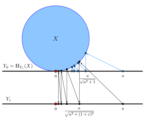
Figure 3: Hölder error bound between $X$ and $\mathds{H}_{Y_{\varepsilon}}(X)$.

We would like to draw our attention to a MAP iteration between $X$ and $Y_{0}$, and one concerning $X$ and $Y_{\varepsilon}$. These MAP iterations are given below and illustrated in Figure 3. For a number $a>0$, consider $(a,0)\in Y_{0}$ and $(a,-\varepsilon)\in Y_{\varepsilon}$. Note that

$$P_{Y_{0}}P_{X}(a,0)=\left(\frac{a}{\sqrt{a^{2}+1}},0\right)\in Y_{0}$$

and

$$P_{Y_{\varepsilon}}P_{X}(a,-\varepsilon)=\left(\frac{a}{\sqrt{a^{2}+(1+\varepsilon)^{2}}},-\varepsilon\right)\in Y_{\varepsilon}.$$

Note also that

$$\lim_{a\to 0^{+}}\frac{\left\lVert P_{Y_{0}}P_{X}(a,0)-(0,0)\right\rVert}{\left\lVert(a,0)-(0,0)\right\rVert}=\lim_{a\to 0^{+}}\frac{1}{\sqrt{a^{2}+1}}=1,$$

and

$$\lim_{a\to 0^{+}}\frac{\left\lVert P_{Y_{\varepsilon}}P_{X}(a,-\varepsilon)-(0,-\varepsilon)\right\rVert}{\left\lVert(a,-\varepsilon)-(0,-\varepsilon)\right\rVert}=\lim_{a\to 0^{+}}\frac{1}{\sqrt{a^{2}+(1+\varepsilon)^{2}}}=\frac{1}{1+\varepsilon}.$$

The limit being $1$ in Example 5.5 means that a MAP sequence between $X$ and $Y_{0}$, monitored on $Y_{0}$, converges to the origin sublinearly. On the other hand, in view of Example 5.5, the gap of size $\varepsilon$ leads to a linear convergence of a MAP sequence to the best point $(0,-\varepsilon)$ with asymptotic rate $\frac{1}{1+\varepsilon}$, where this MAP sequence regards $X$ and $Y_{\varepsilon}$ and belongs to $Y_{\varepsilon}$. For simplicity, we are looking at MAP shadows on $Y_{0}$/$Y_{\varepsilon}$, but of course, due to the nonexpansiveness of projections, the rates would be sublinear/linear for the correspondent shadows on $X$.

Apparently, this leap from sublinear to linear convergence occurs in view of the presence of a Hölder error bound condition between $X$ and $\mathds{H}_{Y_{\varepsilon}}(X)$. In fact, we have the existence of $\omega>0$ such that

$$\omega\operatorname{dist}(x,X\cap\mathds{H}_{Y_{\varepsilon}}(X))^{1+q}\leq\operatorname{dist}(x,\mathds{H}_{Y_{\varepsilon}}(X)),$$

$x\in X$ in a neighborhood of $X\cap\mathds{H}_{Y_{\varepsilon}}(X)=\{(0,0)\}$, with $q=1$. We remark that the Hölder parameter $q=1$ can be effortlessly derived in this example by taking into account that $X$ is entirely contained in the epigraph of the quadratic function $g(t)=\frac{t^{2}}{2}$.

The previous example presented a particular instance where adding inconsistency led to a gain in the convergence rate of MAP from sublinear to linear. We understand this is not something one can expect without assuming some Hölder regularity. Probably, the improvement of MAP would be more limited if we considered MAP for a Cauchy bowl getting apart from a hyperplane. By Cauchy bowl [3] we mean something like the epigraph of the function $f:D\to\mathds{R}$ defined such that $f(0)=0$ and $f(x)=e^{{\left\lVert x\right\rVert}^{-2}}$ elsewhere, where $D=\{x\in\mathds{R}^{n}\mid\left\lVert x\right\rVert\leq 1/\sqrt{3}\}$. This function $f$ is known to be infinitely differentiable in the interior of its domain, but not analytic. Furthermore, its epigraph does not satisfy a Hölder error bound with respect to the hyperplane $H=\left\{(x,0)\in\mathds{R}^{n+1}\mid x\in\mathds{R}^{n}\right\}$.

We have just risen the conjecture of whether Hölder regularity, with $q=1$, provides linear convergence for MAP in the inconsistent case. This looks very plausible and if indeed correct, it can establish MAP as a practical and (perhaps) competitive method for non-smooth optimization, at least for convex min-max problems featuring convex quadratic functions. Perhaps KŁ-theory [5, 46] may shed some light on the question.

Example 5.6 (MAP for convex min-max optimization).

Consider the following problem

$$\min_{x\in\mathds{R}^{n}}g(x)\coloneqq\max\left\{f_{1}(x),\ldots,f_{m}(x)\right\},$$

where each $f_{i}:\mathds{R}^{n}\to\mathds{R}$ is a convex function and assume that $g$ has a minimizer. Let $g^{*}$ be the optimal value of Example 5.6, take $\beta<g^{*}$ and define the hyperplane $H_{\beta}\coloneqq\{(x,\beta)\in\mathds{R}^{n+1}\mid x\in\mathds{R}^{n}\}$. Thus, the epigraph of $g$, $\operatorname{epi}g\coloneqq\{(x,t)\in\mathds{R}^{n+1}\mid x\in\mathds{R}^{n},g(x)\leq t\}$, does not intersect $H_{\beta}$ and $\operatorname{bap}_{H_{\beta}}(\operatorname{epi}g)$ consists of the minimizers of $g$. Moreover, due to Fact 3(i), for any starting point $(x^{0},t_{0})\in\mathds{R}^{n+1}$ the MAP sequence defined by

$$(x^{k+1},t_{k+1})\coloneqq P_{\operatorname{epi}g}P_{H_{\beta}}((x^{k},t_{k}))$$

converges to a point $(x^{*},g^{*})$ such that $x^{*}$ is a solution of Example 5.6.

Note that if all $f_{i}$ are affine, solving Example 5.6 relates to linear programming, in the sense discussed in Example 5.1, and finite convergence of the MAP sequence Example 5.6 is assured by Theorem 4.1.

Now, Theorem 4.3 opens the possibility for the MAP sequence Example 5.6 to achieve finite convergence in a more general setting. If, for instance, the solution $x^{*}$ of Example 5.6 is unique and if the tangent cone of $\operatorname{epi}g$ at $(x^{*},g^{*})$ is pointed, the Lipschitzian BAP-EB Lemma 3.5 holds and the MAP sequence Example 5.6 converges to $(x^{*},g^{*})$ after a finite number of steps.

Of course that addressing a non-affine setting in practice relies on the calculation of projections onto epigraphs and a lower bound $\beta$ for $g$ in hand. Getting $\beta$ is potentially an easier task. For instance, if there is an index $\hat{\imath}$ for which $f_{\hat{\imath}}$ has a minimizer $\hat{x}$, we have that any $\beta<f_{\hat{\imath}}(\hat{x})$ provides a strict lower bound for $g$ as $f_{\hat{\imath}}(\hat{x})\leq g^{*}$.

With that said, one can think of using MAP for quadratic min-max, that is, when all $f_{i}$’s are convex quadratic functions. In this case, finding $\beta$ is easy and projecting onto the epigraph of $g$ is somehow manageable [32]. As for the BAP-EB  Lemma 3.5, it may or may not be satisfied. However, the Hölder condition Example 5.5 holds with $q=1$, in view of the quadratic growth of $g$. Hence, if the conjecture raised in Example 5.5 is true for $q=1$, we would get either finite or linear convergence of the MAP sequence Example 5.6 for convex quadratic min-max problems.

Furthermore, the conjecture being true would echo as well in min-max problems featuring strongly convex functions. The maximum of a finite number of strongly convex functions is strongly convex, has a unique minimizer and one can bound $g$ below by a strictly convex quadratic function with minimum value $g^{*}$. So, Hölder regularity holds with $q=1$ in the strongly convex setting of Example 5.6 and again, one would either get finite or linear convergence of the MAP sequence Example 5.6.

The bonds between min-max problems and Hölder regularity together with the validity of the conjecture formulated in Example 5.5 would be an asset in the field of non-smooth convex optimization.

6 Concluding remarks

We have derived finite convergence of alternating projections for two non-intersecting closed convex sets satisfying a Lipschitzian error bound condition, which has been to proven be more general than the well known concept of intrinsic transversality. This result strengthens the theory on MAP, a widely acclaimed method in Mathematics. In addition to being interesting from a theoretical point of view, our main theorem may also have an impact on practical issues regarding projection-type algorithms in general, as inconsistency has been seen favorable for MAP. A question left open is to what extent MAP can improve when embedding inconsistency to a problem satisfying a Hölder error bound condition. As discussed within an example, a positive answer in this direction may turn MAP into an attractive method for minimizing the maximum of convex functions, a central problem in non-smooth optimization. Although our main results are for finite convergence of MAP, we have as well stated theorems on other projection/reflection-based methods for both two-set and multi-set inconsistent feasibility problems. In particular, the Cimmino method, the Douglas-Rachford method and Cyclic projections have been addressed.

References

- [1] R. Aharoni, Y. Censor, and Z. Jiang, Finding a best approximation pair of points for two polyhedra, Comput Optim Appl, 71 (2018), pp. 509–523, https://doi.org/10.1007/s10589-018-0021-3.
- [2] S. Alwadani, H. H. Bauschke, J. P. Revalski, and X. Wang, The difference vectors for convex sets and a resolution of the geometry conjecture, arXiv:2012.04784 [math], (2020), https://arxiv.org/abs/2012.04784.
- [3] R. Arefidamghani, R. Behling, J.-Y. Bello-Cruz, A. N. Iusem, and L.-R. Santos, The circumcentered-reflection method achieves better rates than alternating projections, Comput Optim Appl, 79 (2021), pp. 507–530, https://doi.org/10.1007/s10589-021-00275-6, https://arxiv.org/abs/2007.14466.
- [4] N. Aronszajn, Theory of Reproducing Kernels, Transactions of the American Mathematical Society, 68 (1950), pp. 337–404, https://doi.org/10.1090/S0002-9947-1950-0051437-7.
- [5] H. Attouch, J. Bolte, P. Redont, and A. Soubeyran, Proximal Alternating Minimization and Projection Methods for Nonconvex Problems: An Approach Based on the Kurdyka-Łojasiewicz Inequality, Mathematics of OR, 35 (2010), pp. 438–457, https://doi.org/10.1287/moor.1100.0449.
- [6] C. Badea, S. Grivaux, and V. Müller, The rate of convergence in the method of alternating projections, St. Petersburg Mathematical Journal, 23 (2012), pp. 413–434, https://doi.org/10.1090/S1061-0022-2012-01202-1.
- [7] J.-B. Baillon, P. Combettes, and R. Cominetti, There is no variational characterization of the cycles in the method of periodic projections, Journal of Functional Analysis, 262 (2012), pp. 400–408, https://doi.org/10.1016/j.jfa.2011.09.002.
- [8] H. H. Bauschke, A norm convergence result on random products of relaxed projections in Hilbert space, Trans. Amer. Math. Soc., 347 (1995), pp. 1365–1373, https://doi.org/10.1090/S0002-9947-1995-1257097-1.
- [9] H. H. Bauschke, J.-Y. Bello-Cruz, T. T. A. Nghia, H. M. Phan, and X. Wang, Optimal Rates of Linear Convergence of Relaxed Alternating Projections and Generalized Douglas-Rachford Methods for Two Subspaces, Numer. Algorithms, 73 (2016), pp. 33–76, https://doi.org/10.1007/s11075-015-0085-4.
- [10] H. H. Bauschke and J. M. Borwein, On the convergence of von Neumann’s alternating projection algorithm for two sets, Set-Valued Analysis, 1 (1993), pp. 185–212, https://doi.org/10.1007/BF01027691.
- [11] H. H. Bauschke and J. M. Borwein, Dykstra′s Alternating Projection Algorithm for Two Sets, J. Approx. Theory, 79 (1994), pp. 418–443, https://doi.org/10.1006/jath.1994.1136.
- [12] H. H. Bauschke and J. M. Borwein, On Projection Algorithms for Solving Convex Feasibility Problems, SIAM Review, 38 (1996), pp. 367–426, https://doi.org/10.1137/S0036144593251710.
- [13] H. H. Bauschke, J. M. Borwein, and A. S. Lewis, The method of cyclic projections for closed convex sets in Hilbert space, Contemporary Math., 204 (1997), pp. 1–38.
- [14] H. H. Bauschke and P. L. Combettes, Convex Analysis and Monotone Operator Theory in Hilbert Spaces, CMS Books in Mathematics, Springer International Publishing, second ed., 2017, https://doi.org/10.1007/978-3-319-48311-5.
- [15] H. H. Bauschke, P. L. Combettes, and D. R. Luke, Finding best approximation pairs relative to two closed convex sets in Hilbert spaces, Journal of Approximation Theory, 127 (2004), pp. 178–192, https://doi.org/10.1016/j.jat.2004.02.006.
- [16] H. H. Bauschke, F. Deutsch, and H. Hundal, Characterizing arbitrarily slow convergence in the method of alternating projections, International Transactions in Operational Research, 16 (2009), pp. 413–425, https://doi.org/10.1111/j.1475-3995.2008.00682.x.
- [17] R. Behling, J.-Y. Bello-Cruz, and L.-R. Santos, The block-wise circumcentered–reflection method, Comput Optim Appl, 76 (2020), pp. 675–699, https://doi.org/10.1007/s10589-019-00155-0.
- [18] R. Behling, D. S. Gonçalves, and S. A. Santos, Local Convergence Analysis of the Levenberg–Marquardt Framework for Nonzero-Residue Nonlinear Least-Squares Problems Under an Error Bound Condition, J Optim Theory Appl, 183 (2019), pp. 1099–1122, https://doi.org/10.1007/s10957-019-01586-9.
- [19] R. Behling and A. Iusem, The effect of calmness on the solution set of systems of nonlinear equations, Math. Program., 137 (2013), pp. 155–165, https://doi.org/10.1007/s10107-011-0486-7.
- [20] D. P. Bertsekas, Nonlinear Programming, Athena Scientific, Belmont, USA, second ed., 1999.
- [21] J. M. Borwein, G. Li, and M. K. Tam, Convergence Rate Analysis for Averaged Fixed Point Iterations in Common Fixed Point Problems, SIAM J. Optim., 27 (2017), pp. 1–33, https://doi.org/10.1137/15M1045223.
- [22] J. M. Borwein, G. Li, and L. Yao, Analysis of the Convergence Rate for the Cyclic Projection Algorithm Applied to Basic Semialgebraic Convex Sets, SIAM J. Optim., 24 (2014), pp. 498–527, https://doi.org/10.1137/130919052.
- [23] H. T. Bui, R. Loxton, and A. Moeini, A note on the finite convergence of alternating projections, Operations Research Letters, 49 (2021), pp. 431–438, https://doi.org/10.1016/j.orl.2021.04.009.
- [24] Y. Censor, On variable block algebraic reconstruction techniques, in Mathematical Methods in Tomography, G. T. Herman, A. K. Louis, and F. Natterer, eds., vol. 1497 of Lecture Notes in Mathematics, Springer, Berlin, Heidelberg, 1991, pp. 133–140, https://doi.org/10.1007/BFb0084514.
- [25] Y. Censor, M. D. Altschuler, and W. D. Powlis, On the use of Cimmino’s simultaneous projections method for computing a solution of the inverse problem in radiation therapy treatment planning, Inverse Problems, 4 (1988), pp. 607–623, https://doi.org/10.1088/0266-5611/4/3/006.
- [26] Y. Censor and A. Cegielski, Projection methods: An annotated bibliography of books and reviews, Optimization, 64 (2014), pp. 2343–2358, https://doi.org/10.1080/02331934.2014.957701.
- [27] Y. Censor and M. Zaknoon, Algorithms and Convergence Results of Projection Methods for Inconsistent Feasibility Problems: A Review, Pure and Applied Functional Analysis, 3 (2018), pp. 565–586.
- [28] W. Cheney and A. A. Goldstein, Proximity Maps for Convex Sets, Proceedings of the American Mathematical Society, 10 (1959), pp. 448–450, https://doi.org/10.2307/2032864.
- [29] G. Cimmino, Calcolo approssimato per le soluzioni dei sistemi di equazioni lineari, La Ricerca Scientifica, 9 (1938), pp. 326–333.
- [30] E. S. Coakley, V. Rokhlin, and M. Tygert, A Fast Randomized Algorithm for Orthogonal Projection, SIAM Journal on Scientific Computing, 33 (2011), pp. 849–868, https://doi.org/10.1137/090779656.
- [31] P. L. Combettes, Inconsistent signal feasibility problems: Least-squares solutions in a product space, IEEE Trans. Signal Process., 42 (1994), pp. 2955–2966, https://doi.org/10.1109/78.330356.
- [32] Y.-H. Dai, Fast Algorithms for Projection on an Ellipsoid, SIAM J. Optim., 16 (2006), pp. 986–1006, https://doi.org/10.1137/040613305.
- [33] A. R. De Pierro and A. N. Iusem, A finitely convergent “row-action” method for the convex feasibility problem, Appl Math Optim, 17 (1988), pp. 225–235, https://doi.org/10.1007/BF01448368.
- [34] F. Deutsch, The Method of Alternating Orthogonal Projections, in Approximation Theory, Spline Functions and Applications, S. P. Singh, ed., no. 356 in NATO ASI Series, Springer, Dordrecht, 1992, pp. 105–121, https://doi.org/10.1007/978-94-011-2634-2_5.
- [35] F. R. Deutsch, The Angle Between Subspaces of a Hilbert Space, in Approximation Theory, Wavelets and Applications, S. P. Singh, ed., vol. 454 of NATO Science Series, Springer, Dordrecht, 1995, pp. 107–130, https://doi.org/10.1007/978-94-015-8577-4_7.
- [36] F. R. Deutsch and H. Hundal, The Rate of Convergence for the Method of Alternating Projections, II, J. Math. Anal. Appl., 205 (1997), pp. 381–405, https://doi.org/10.1006/jmaa.1997.5202.
- [37] P. Diaconis, K. Khare, and L. Saloff-Coste, Stochastic alternating projections, Illinois J. Math., 54 (2010), pp. 963–979, https://doi.org/10.1215/ijm/1336568522.
- [38] J. Douglas and H. H. Rachford Jr., On the numerical solution of heat conduction problems in two and three space variables, Transactions of the American Mathematical Society, 82 (1956), pp. 421–421, https://doi.org/10.1090/S0002-9947-1956-0084194-4.
- [39] D. Drusvyatskiy, A. D. Ioffe, and A. S. Lewis, Transversality and Alternating Projections for Nonconvex Sets, Found Comput Math, 15 (2015), pp. 1637–1651, https://doi.org/10.1007/s10208-015-9279-3.
- [40] D. Drusvyatskiy, G. Li, and H. Wolkowicz, A note on alternating projections for ill-posed semidefinite feasibility problems, Mathematical Programming, 162 (2016), pp. 537–548, https://doi.org/10.1007/s10107-016-1048-9.
- [41] C. Franchetti and W. Light, On the von Neumann alternating algorithm in Hilbert space, J. Math. Anal. Appl., 114 (1986), pp. 305–314, https://doi.org/10.1016/0022-247X(86)90085-5.
- [42] L. G. Gubin, B. T. Polyak, and E. V. Raik, The method of projections for finding the common point of convex sets, USSR Computational Mathematics and Mathematical Physics, 7 (1967), pp. 1–24, https://doi.org/10.1016/0041-5553(67)90113-9.
- [43] S. Kaczmarz, Angenäherte Auflösung von Systemen linearer Gleichungen, Bull. Int. Acad. Pol. Sci. Lett. Class. Sci. Math. Nat. A, 35 (1937), pp. 355–357.
- [44] S. Kayalar and H. L. Weinert, Error bounds for the method of alternating projections, Math. Control Signal Systems, 1 (1988), pp. 43–59, https://doi.org/10.1007/BF02551235.
- [45] A. Y. Kruger, About Intrinsic Transversality of Pairs of Sets, Set-Valued Var. Anal, 26 (2018), pp. 111–142, https://doi.org/10.1007/s11228-017-0446-3.
- [46] G. Li and T. K. Pong, Calculus of the Exponent of Kurdyka–Łojasiewicz Inequality and Its Applications to Linear Convergence of First-Order Methods, Found Comput Math, 18 (2018), pp. 1199–1232, https://doi.org/10.1007/s10208-017-9366-8.
- [47] E. A. Nurminski, Single-projection procedure for linear optimization, J Glob Optim, 66 (2016), pp. 95–110, https://doi.org/10.1007/s10898-015-0337-9.
- [48] G. Pierra, Decomposition through formalization in a product space, Mathematical Programming, 28 (1984), pp. 96–115, https://doi.org/10.1007/BF02612715.
- [49] R. T. Rockafellar and R. J.-B. Wets, Variational Analysis, no. 317 in Grundlehren Der Mathematischen Wissenschaften, Springer, Berlin, second ed., 2004.
- [50] K. T. Smith, D. C. Solmon, and S. L. Wagner, Practical and mathematical aspects of the problem of reconstructing objects from radiographs, Bull. Amer. Math. Soc., 83 (1977), pp. 1227–1271, https://doi.org/10.1090/S0002-9904-1977-14406-6.
- [51] J. von Neumann, Functional Operators, Volume 2: The Geometry of Orthogonal Spaces., no. 22 in Annals of Mathematics Studies, Princeton University Press, Princeton, 1950, https://doi.org/10.2307/j.ctt1bc543b.