Reliable Liver Fibrosis Assessment from Ultrasound using Global Hetero-Image Fusion and View-Specific Parameterization

Abstract

US is a critical modality for diagnosing liver fibrosis. Unfortunately, assessment is very subjective, motivating automated approaches. We introduce a principled deep NN workflow that incorporates several innovations. First, to avoid overfitting on non-relevant image features, we force the network to focus on a clinical ROI, encompassing the liver parenchyma and upper border. Second, we introduce HVF, which allows the NN to fuse features from any arbitrary number of images in a study, increasing its versatility and flexibility. Finally, we use “style”-based VSP to tailor the NN processing for different viewpoints of the liver, while keeping the majority of parameters the same across views. Experiments on a dataset of $610$ patient studies ($6979$ images) demonstrate that our pipeline can contribute roughly $7\%$ and $22\%$ improvements in partial AUC and R@P90, respectively, over conventional classifiers, validating our approach to this crucial problem.

1 Introduction

Liver fibrosis is a major health threat with high prevalence [19]. Without timely diagnosis and treatment, liver fibrosis can develop into liver cirrhosis [19] and even hepatocellular carcinoma [21]. While histopathology remains the gold standard, non-invasive approaches minimize patient discomfort and danger. Elastography is a useful non-invasive modality, but it is not always available or affordable and it can be confounded by inflammation, presence of steatosis, and the patient’s etiology [23, 2, 12]. Assessment using conventional US may be potentially more versatile; however, it is a subjective measurement that can suffer from insufficient sensitivities, specificities, and high inter- and intra-rater variability [15, 13]. Thus, there is great impetus for an automated and less subjective assessment of liver fibrosis. This is the goal of our work.

Although a relatively understudied topic, prior work has advanced automated US fibrosis assessment [17, 4, 18, 16, 14]. In terms of deep NN, Meng et al. [16] proposed a straightforward liver fibrosis parenchyma VGG-16-based [22] classifier and tested it on a small dataset of $279$ images. Importantly, they only performed image-wise predictions and do not report a method for study-wise classification. On the other hand, Liu et al. [14] correctly identified the value in fusing features from all US images in a study when making a prediction. However, their algorithm requires exactly $10$ images. But, real patient studies may contain any arbitrary number of US scans. Their feature concatenation approach would also drastically increase computational and memory costs as more images are incorporated. Moreover, they rely on $13$ manually labeled indicators as ancillary supervision, which are typically not available without considerable labor costs. Finally, their system treats all US images identically, even though a study consists of different viewpoints of the liver, each of which may have its own set of clinical markers correlating with fibrosis. Ideally, a liver fibrosis assessment system could learn directly from supervisory signals already present in hospital archives, i.e., image-level fibrosis scores produced during daily clinical routines. In addition, a versatile system should also be able to effectively use all US images/views in a patient study with no ballooning of computational costs, regardless of their number.

We fill these gaps by proposing a robust and versatile pipeline for conventional ultrasound liver fibrosis assessment. Like others, we use a deep NN, but with key innovations. First, informed by clinical practice [1], we ensure the network focuses only on a clinically-important ROI, i.e., the liver parenchyma and the upper liver border. This prevents the NN from erroneously overfitting on spurious or background features. Second, inspired by HeMIS [6], we adapt and expand on this approach and propose HVF as a way to learn from, and perform inference on, any arbitrary number of US scans within a study. While HVF share similarities with deep feature-based multi-instance learning [10], there are two important distinctions: (1) HVF includes variance as part of the fusion, as per HeMIS [6]; (2) HVF is trained using arbitrary image combinations from a patient study, which is possible because, unlike multi-instance learning, each image (or instance) is strongly supervised by the same label. We are the first to propose and develop this mechanism to fuse global NN feature vectors. Finally, we implement a VSP that tailors the NN processing based on $6$ common liver US views. While the majority of processing is shared, each view possesses its own set of so-called “style”-based normalization parameters [9] to customize the analysis. While others have used similar ideas segmenting different anatomical structures [8], we are the first to apply this concept for clinical decision support and the first to use it in concert with a hetero-image fusion mechanism. The result is a highly robust and practical liver fibrosis assessment solution.

To validate our approach, we use a cross-validated dataset of $610$ US patient studies, comprising $6976$ images. We measure the ability to identify patients with moderate to severe liver fibrosis. Compared to strong classification baselines, our enhancements are able to improve recall at $90\%$ precision by $22\%$, with commensurate boosts in partial AUC. Importantly, ablation studies demonstrate that each component contributes to these performance improvements, demonstrating that our liver fibrosis assessment pipeline, and its constituent clinical ROI, HVF, and VSP parts, represents a significant advancement for this important task.

2 Methods

We assume we are given a dataset, $\mathcal{D}=\{\mathcal{X}_{i},y_{i}\}_{i=1}^{N}$, comprised of US patient studies and ground-truth labels indicating liver fibrosis status, dropping the $i$ when convenient. Each study $\mathcal{X}_{i}$, in turn, is comprised of an arbitrary number of $K_{i}$ 2D conventional US scans of the patient’s liver, $\mathcal{X}_{i}=\{\mathbf{X}^{1}\ldots\mathbf{X}^{K_{i}}\}$. Fig. 1 depicts the workflow of our automated liver assessment tool, which combines clinical ROI pooling, HVF, and VSP.

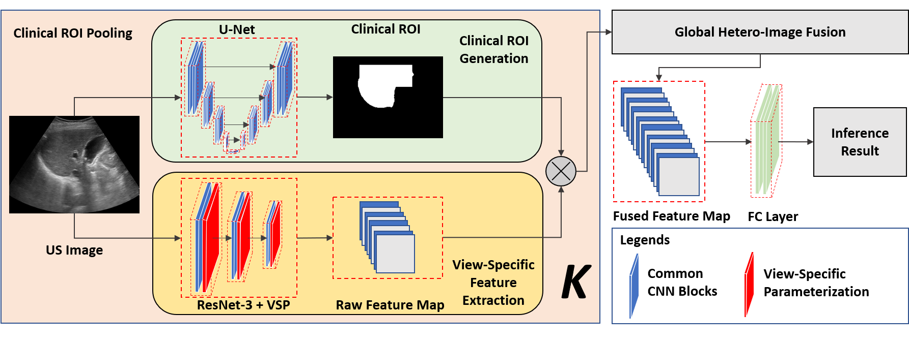
Figure 1: Algorithmic workflow depicting the clinical ROI pooling, HVF, and VSP. We use plate notation to depict the repeated workflow across the $K$ images in a US study.

2.1 Clinical ROI Pooling

We use a deep NN as backbone for our pipeline. Popular deep NN, e.g., ResNet [7], can be formulated with the following convention:

$$\hat{y}^{k} =f\left(g\left(\mathbf{A}^{k}\right);\mathbf{w}\right)\mathrm{,}$$ (1)

$$\mathbf{A}^{k} =h\left(\mathbf{X}^{k};\theta\right)\mathrm{,}$$ (2)

where $h(.;\theta)$ is a FCN feature extractor parameterized by $\theta$, $\mathbf{A}^{k}$ is the FCN output, $g(.)$ is some global pooling function, e.g., average pooling, and $f(.;\mathbf{w})$ is a fully-connected layer (and sigmoid function) parameterized by $\mathbf{w}$. When multiple US scans are present, a standard approach is to aggregate individual image-wise predictions, e.g., taking the median:

$$\hat{y}=\mathrm{median}(\{\hat{y}^{1}\ldots\hat{y}^{K}\})\mathrm{.}$$ (3)

This conventional approach may have drawbacks, as it is possible for the NN to overfit to spurious background variations. However, based on clinical practice [1], we know a priori that certain features are crucial for assessing liver fibrosis, e.g., the parenchyma texture and surface nodularity. As Fig. 2 demonstrates, to make the NN focus on these features we use a masking technique. We first generate a liver mask for each US scan. This is done by training a simple segmentation network on a small subset of the images.

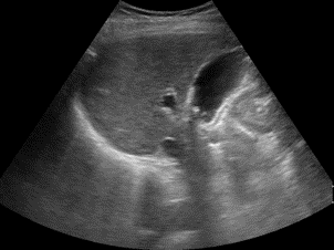
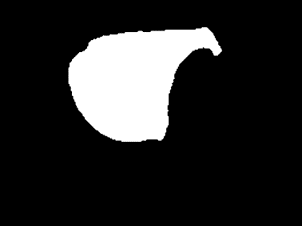
(a) US Image	(b) Liver Mask	(c) Clinical ROI

Figure 2: (a) depicts an US image, whose liver mask is rendered in (b). As shown in (c), the clinical ROI the mask is extended upward to cover the top liver border.

Then, for each scan, we create a rectangle that just covers the top half of and 10 pixels above the liver mask, to ensure the liver border is covered. The resulting binary mask is denoted $\mathbf{M}$. Because we only need to ensure we capture enough of the liver parenchyma and upper border to extract meaningful features, $\mathbf{M}$ need not be perfect.

With a clinical ROI obtained, we formulate the pooling function in (1) as a masked version of global average pooling:

$$g(\mathbf{A};\mathbf{M})=\mathrm{GAP}(\mathbf{M}\odot\mathbf{A})\mathrm{,}$$ (4)

where $\odot$ and $\mathrm{GAP}(.)$ denote the element-wise product and global average pooling, respectively. Interestingly, we found that including the zeroed-out regions within the global average pooling benefits performance [3, 25]. We posit their inclusion helps implicitly capture liver size characteristics, which is another important clinical US marker for liver fibrosis [1].

2.2 Global Hetero-Image Fusion

A challenge with US patient studies is that they may consist of a variable number of images, each of a potentially different view. Ideally, all available US images would contribute to the final prediction. In (3) this is accomplished via a late fusion of independent and image-specific predictions. But, this does not allow the NN integrate the combined features across US images. A better approach would fuse these features. The challenge, here, is to allow for an arbitrary number of US images in order to ensure flexibility and practicality.

The HeMIS approach [6] to segmentation offers a promising strategy that fuses features from arbitrary numbers of images using their first- and second-order moments. However, HeMIS fuses convolutional features early in its FCN pipeline, which is possible because it assumes pixel-to-pixel correspondence across images. This is completely violated for US images. Instead, only global US features can be sensibly fused together, which we accomplish through HVF. More formally, we use $\mathcal{A}=\{\mathbf{A}^{k}\}_{k=1}^{K}$ and $\mathcal{M}=\{\mathbf{M}^{k}\}_{k=1}^{K}$ to denote the set of FCN features and clinical ROI, respectively, for each image. Then HVF modifies (1) to accept any arbitrary set of FCN features to produce a study-wise prediction:

$$\hat{y} =f\left(g\left(\mathcal{A};\mathcal{M}\right);\mathbf{w}\right)\mathrm{,}$$ (5)

$$g(\mathcal{A};\mathcal{M}) =\mathrm{concat}\left(\mathrm{mean}(\mathcal{G}),\mathrm{var}(\mathcal{G}),\max(\mathcal{G})\right)\mathrm{,}$$ (6)

$$\mathcal{G} =\{\mathrm{GAP}(\mathbf{M}^{k}\odot\mathbf{A}^{k})\}_{k=1}^{K}\mathrm{,}$$ (7)

Besides the first- and second-order moments, HVF (6) also incorporates the max operator as a powerful hetero-fusion function [26]. All three operators can accept any arbitrary numbers of samples to produce one fused feature vector. To the best of our knowledge, we are the first to apply hetero-fusion for global feature vectors. The difference, compared to late fusion, is that features, rather than predictions are fused. Rather than always inputting all US scans when training, an important strategy is choosing random combinations of the $K$ scans for every epoch. This provides a form of data augmentation and allows the NN to learn from image signals that may be suppressed otherwise. An important implementation note is that training with random combinations of images can make HVF’s batch statistics unstable. For this reason, a normalization not relying on batch statistics, such as instance-normalization [24], should be used.

2.3 View-Specific Parameterization

While HVF can effectively integrate arbitrary numbers of US images within a study, it uses the same FCN feature extractor across all images, treating them all identically. Yet, there are certain US features, such as vascular markers, that are specific to particular views. As a result, some manner of view-specific analysis could help push performance further. In fact, based on guidance from our clinical partner, US views of the liver can be roughly divided into $6$ categories, which focus on different regions of the liver. These are shown in Fig 3.

Figure 3: Liver views in our dataset. Blue square: position of the US probe. Liver cartoons adapted from the DataBase Center for Life Science (https://commons.wikimedia.org/wiki/File:201405_liver.png), licensed under the Creative Commons Attribution 4.0 International

A naive solution would be to use a dedicated deep NN for each view category. However, this would drastically reduce the training set for each dedicated NN and would sextuple the number of parameters, computation, and memory consumption. Intuitively, there should be a great deal of analysis that is common across US views. The challenge is to retain this shared analysis, while also providing some tailored processing for each category.

To do this, we adapt the concept of “style” parameters to implement a VSP appropriate for US-based fibrosis assessment. Such parameters refer to the affine normalization parameters used in batch- [11] or instance-normalization [24]. If these are switched out, while keeping all other parameters constant, one can alter the behavior of the NN in quite dramatic ways [9, 8]. For our purposes, retaining view-specific normalization parameters allows for the majority of parameters and processing to be shared across views. VSP is then realized with a minimal number of additional parameters.

More formally, if we create $6$ sets of normalization parameters for an FCN, we can denote them as $\Omega=\{\omega_{1}\ldots\omega_{6}\}$. The FCN from (2) is then modified to be parameterized also by $\Omega$:

$$\mathbf{A}^{k} =h\left(\mathbf{X}^{k};\theta,\omega_{v_{k}}\right)\mathrm{,}$$ (8)

where $v_{k}$ indexes each image by its view and $\theta$ now excludes the normalization parameters. VSP relies on identifying the view of each US scan in order to swap in the correct normalization parameters. This can be recorded as part of the acquisition process. Or, if this is not possible, we have found classifying the US views automatically to be quite reliable.

3 Experiments

Dataset. We test our system on a dataset of $610$ US patient studies collected from the Chang Gung Memorial Hospital in Taiwan, acquired from Siemens, Philips, and Toshiba devices. The dataset comprises $232$ patients, among which $95$ ($40.95\%$) patients have moderate to severe fibrosis (27 with severe liver steatosis). All patients were diagnosed with hepatitis B. Patients were scanned up to $3$ times, using a different scanner type each time. Each patient study is composed of up to $14$ US images, corresponding to the views in Fig. 3. The total number of images is $6\,979$. We use $5$-fold cross validation, splitting each fold at the patient level into $70\%$, $20\%$, and $10\%$, for training, testing, and validation, respectively. We also manually labeled liver contours from $300$ randomly chosen US images.

Implementation Details and Comparisons. Experiments evaluated our workflow against several strong classification baselines, where throughout we use the same ResNet50 [7] backbone (pretrained on ImageNet [5]). For methods using the clinical ROI pooling of (4), we use a truncated version of ResNet (only the first three layer blocks) for $h(.)$ in (2). This keeps enough spatial resolution prior to the masking in (4). We call this truncated backbone “ResNet-3”. To create the clinical ROI, we train a simple 2D U-Net [20] on the $300$ images with masks. For training, we perform standard data augmenation with random brightness, contrast, rotations, and scale adjustments. We use the stochastic gradient descent optimizer and a learning rate of 0.001 to train all networks.

Table 1: Ablation Studies

Method	Partial AUC	AUC	R@P90	R@P85	R@P80
ResNet50	$0.710$	$0.893$	$41.0\%$	$61.7\%$	$74.6\%$
Clinical ROI	$0.744$	$0.908$	$46.1\%$	$59.2\%$	$82.1\%$
Global Fusion	$0.591$	$0.845$	$30.2\%$	$36.0\%$	$49.8\%$
GHIF	$0.691$	$0.885$	$36.7\%$	$41.0\%$	$65.0\%$
GHIF (I-Norm)	$0.762$	$0.907$	$57.1\%$	$71.1\%$	$80.6\%$
GHIF + VSP (I-Norm)	$\mathbf{0.783}$	$\mathbf{0.913}$	$\mathbf{63.4\%}$	$\mathbf{78.3\%}$	$\mathbf{84.2\%}$

For baselines that can output only image-wise predictions, we test against a conventional ResNet50 and also a ResNet-3 with clinical ROI pooling. For these two approaches, following clinical practices, we take the median value across the image-wise predictions to produce a study-wise prediction. All subsequent study-wise baselines are then built off the ResNet-3 with clinical ROI pooling. We first test the global feature fusion of (6), but only train the ResNet-3 with all available images in a US study. In this way, it follows the spirit of Liu et al.’s global fusion strategy [14]. To reveal the impact of our hetero-fusion training strategy that uses different random combinations of US images per epoch, we also test two HVF variants, one using batch-normalization and one using instance-normalization. The latter helps measure the importance of using proper normalization strategies to manage the instability of HVF’s batch statistics. Finally, we test our proposed model which incorporates VSP on top of HVF and clinical ROI pooling.

Evaluation Protocols. The problem setup is binary classification, i.e., identifying patients with moderate to severe liver fibrosis, which are the patient cohorts requiring intervention. While we report full AUC, we primarily focus on operating points within a useful range of specificity or precision. Thus, we evaluate using partial AUC that only consider false positive rates within $0$ to $30\%$ because higher values lose their practical usefulness. Partial AUC are normalized to be within a range of $0$ to $1$. We also report recalls at a range of precision points (R@P90, R@P85, R@P80) to reveal the achievable sensitivity at high precision points. We report mean values and mean graphs across all cross-validation folds.

Results. Tab. 1 presents our AUC, partial AUC and recall values, whereas Fig. 4 graphs the partial ROC. Several conclusions can be drawn. First, clinical ROI pooling produces significant boosts in performance, validating our strategy of forcing the network to focus on important regions of the image. Second, not surprisingly, global fusion without training with random combinations of images, performs very poorly, as only presenting all study images during training severely limits the data size and variability, handicapping the model.

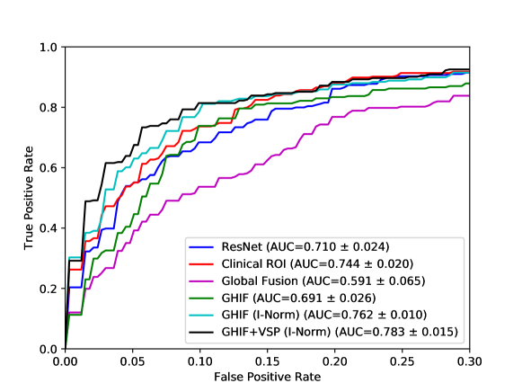
Figure 4: Partial ROC curves are graphed, with corresponding partial AUC found in the legend. Partial AUC scores have been normalized to range from $0-1$. Both ROC and AUC correspond to mean measures taken across the cross-validation folds.

For instance, compared to variants that train on individual images, global fusion effectively reduces the training size by about a factor of $10$ in our dataset. In contrast, the HVF variants, which train with the combinatorial number of random combinations of images, not only avoids drastically reducing the training set size, but can effectively increase it. Importantly, as the table demonstrates, using an appropriate choice of instance normalization is crucial in achieving good performance with HVF. Although not shown, switching to instance normalization did not improve performance for the image-wise or global fusion models. The boosts in HVF performance is apparent in the partial AUC and recalls at high precision points, underscoring the need to analyze results at appropriate operating points. Finally, adding the VSP provides even further performance improvements, particularly in R@P80-R@P90 values, which see a roughly $4-7\%$ increase over HVF alone. This indicates that VSP can significantly enhance the recall at the very demanding precision points necessary for clinical use. In total, compared to a conventional classifier, the enhancements we articulate contribute to roughly $8\%$ improvements in partial AUC and $22\%$ in R@P90 values. Table 1 of our supplementary material also presents AUC when only choosing to input one particular view in the model during inference. We note that performance is highest when all views are inputted into the model, indicating that our pipeline is able to usefully exploit the information across views. Our supplementary also includes liver segmentation results and success and failure cases for our system.

4 Conclusion

We presented a principled and effective pipeline for liver fibrosis characterization from US studies, proposing several innovations: (1) clinical ROI pooling to discourage the network from focusing on spurious image features; (2) HVF to manage any arbitrary number of images in the US study in both training and inference; and (3) VSP to tailor the analysis based on the liver view being presented using “style”-based parameters. In particular, we are the first to propose a deep global hetero-fusion approach and the first to combine it with VSP. Experiments demonstrate that our system can produce gains in partial AUC and R@P90 of roughly $7\%$ and $22\%$, respectively on a dataset of $610$ patient studies. Future work should expand to other liver diseases and more explicitly incorporate other clinical markers, such as absolute or relative liver lobe sizing.

References

- [1] Aubé, C., Bazeries, P., Lebigot, J., Cartier, V., Boursier, J.: Liver fibrosis, cirrhosis, and cirrhosis-related nodules: Imaging diagnosis and surveillance. Diagnostic and Interventional Imaging 98(6), 455 – 468 (2017)
- [2] Chen, C.J., Tsay, P.K., Huang, S.F., Tsui, P.H., Yu, W.T., Hsu, T.H., Tai, J., Tai, D.I.: Effects of hepatic steatosis on non-invasive liver fibrosis measurements between hepatitis b and other etiologies. Applied Sciences 9, 1961 (05 2019)
- [3] Chen, H., Wang, Y., Zheng, K., Li, W., Cheng, C.T., Harrison, A.P., Xiao, J., Hager, G.D., Lu, L., Liao, C.H., Miao, S.: Anatomy-aware siamese network: Exploiting semantic asymmetry for accurate pelvic fracture detection in x-ray images (2020)
- [4] Chung-Ming Wu, Yung-Chang Chen, Kai-Sheng Hsieh: Texture features for classification of ultrasonic liver images. IEEE Transactions on Medical Imaging 11(2), 141–152 (1992)
- [5] Deng, J., Dong, W., Socher, R., Li, L.J., Li, K., Fei-Fei, L.: ImageNet: A Large-Scale Hierarchical Image Database. In: CVPR09 (2009)
- [6] Havaei, M., Guizard, N., Chapados, N., Bengio, Y.: Hemis: Hetero-modal image segmentation. In: Medical Image Computing and Computer-Assisted Intervention. pp. 469–477. Springer (2016)
- [7] He, K., Zhang, X., Ren, S., Sun, J.: Deep residual learning for image recognition. In: 2016 IEEE Conference on Computer Vision and Pattern Recognition, CVPR 2016, Las Vegas, NV, USA, June 27-30, 2016. pp. 770–778 (2016)
- [8] Huang, C., Han, H., Yao, Q., Zhu, S., Zhou, S.K.: 3d u2-net: A 3d universal u-net for multi-domain medical image segmentation. In: Medical Image Computing and Computer Assisted Intervention. pp. 291–299 (2019)
- [9] Huang, X., Belongie, S.: Arbitrary style transfer in real-time with adaptive instance normalization. In: ICCV (2017)
- [10] Ilse, M., Tomczak, J.M., Welling, M.: Attention-based deep multiple instance learning. arXiv preprint arXiv:1802.04712 (2018)
- [11] Ioffe, S., Szegedy, C.: Batch normalization: Accelerating deep network training by reducing internal covariate shift. In: 32nd International Conference on Machine Learning. pp. 448–456 (2015)
- [12] Lee, C.H., Wan, Y.L., Hsu, T.H., Huang, S.F., Yu, M.C., Lee, W.C., Tsui, P.H., Chen, Y.C., Tai, D.I.: Interpretation us elastography in chronic hepatitis b with or without anti-hbv therapy. Applied Sciences 7, 1164 (Nov 2017)
- [13] Li, S., Sun, X., Chen, M., Ying, Z., Wan, Y., Pi, L., Ren, B., Cao, Q.: Liver fibrosis conventional and molecular imaging diagnosis update. Journal of liver 8 (01 2019)
- [14] Liu, J., Wang, W., Guan, T., Zhao, N., Han, X., Li, Z.: Ultrasound liver fibrosis diagnosis using multi-indicator guided deep neural networks. In: Machine Learning in Medical Imaging. pp. 230–237 (2019)
- [15] Manning, D., Afdhal, N.: Diagnosis and quantitation of fibrosis. Gastroenterology 134(6), 1670–1681 (2008)
- [16] Meng, D., Zhang, L., Cao, G., Cao, W., Zhang, G., Hu, B.: Liver fibrosis classification based on transfer learning and fcnet for ultrasound images. IEEE Access 5, 5804–5810 (2017)
- [17] Mojsilovic, A., Markovic, S., Popovic, M.: Characterization of visually similar diffuse diseases from b-scan liver images with the nonseparable wavelet transform. In: Proceedings of International Conference on Image Processing. vol. 3, pp. 547–550 vol.3 (1997)
- [18] Ogawa, K., Fukushima, M., Kubota, K., Hisa, N.: Computer-aided diagnostic system for diffuse liver diseases with ultrasonography by neural networks. IEEE Transactions on Nuclear Science 45(6), 3069–3074 (Dec 1998)
- [19] Poynard, T., Lebray, P., Ingiliz, P., Varaut, A., Varsat, B., Ngo, Y., Norha, P., Munteanu, M., Drane, F., Messous, D., Imbert-Bismut, F., Carrau, J., Massard, J., Ratziu, V., Giordanella, J.: Prevalence of liver fibrosis and risk factors in a general population using non-invasive biomarkers (fibrotest). BMC gastroenterology 10, 40 (04 2010)
- [20] Ronneberger, O., Fischer, P., Brox, T.: U-net: Convolutional networks for biomedical image segmentation. In: Medical Image Computing and Computer-Assisted Intervention. pp. 234–241 (2015)
- [21] Saverymuttu, S.H., Joseph, A.E., Maxwell, J.D.: Ultrasound scanning in the detection of hepatic fibrosis and steatosis. BMJ 292(6512), 13–15 (1986)
- [22] Simonyan, K., Zisserman, A.: Very deep convolutional networks for large-scale image recognition. In: International Conference on Learning Representations (2015)
- [23] Tai, D.I., Tsay, P.K., Jeng, W.J., Weng, C.C., Huang, S.F., Huang, C.H., Lin, S.M., Chiu, C.T., Chen, W.T., Wan, Y.L.: Differences in liver fibrosis between patients with chronic hepatitis b and c. Journal of Ultrasound in Medicine 34(5), 813–821 (2015)
- [24] Ulyanov, D., Vedaldi, A., Lempitsky, V.S.: Instance normalization: The missing ingredient for fast stylization. CoRR abs/1607.08022 (2016)
- [25] Wang, Y., Lu, L., Cheng, C.T., Jin, D., Harrison, A.P., Xiao, J., Liao, C.H., Miao, S.: Weakly supervised universal fracture detection in pelvic x-rays. In: Shen, D., Liu, T., Peters, T.M., Staib, L.H., Essert, C., Zhou, S., Yap, P.T., Khan, A. (eds.) Medical Image Computing and Computer Assisted Intervention – MICCAI 2019. pp. 459–467. Springer International Publishing, Cham (2019)
- [26] Zhou, Y., Li, Y., Zhang, Z., Wang, Y., Wang, A., Fishman, E.K., Yuille, A.L., Park, S.: Hyper-pairing network for multi-phase pancreatic ductal adenocarcinoma segmentation. In: Medical Image Computing and Computer Assisted Intervention. pp. 155–163 (2019)