Rank-based Estimation under Asymptotic Dependence and Independence, with Applications to Spatial Extremes

Abstract

Multivariate extreme value theory is concerned with modeling the joint tail behavior of several random variables. Existing work mostly focuses on asymptotic dependence, where the probability of observing a large value in one of the variables is of the same order as observing a large value in all variables simultaneously. However, there is growing evidence that asymptotic independence is equally important in real world applications. Available statistical methodology in the latter setting is scarce and not well understood theoretically. We revisit non-parametric estimation and introduce rank-based M-estimators for parametric models that simultaneously work under asymptotic dependence and asymptotic independence, without requiring prior knowledge on which of the two regimes applies. Asymptotic normality of the proposed estimators is established under weak regularity conditions. We further show how bivariate estimators can be leveraged to obtain parametric estimators in spatial tail models, and again provide a thorough theoretical justification for our approach.

, and

1 Introduction

Assessing the frequency of extreme events is crucial in many different fields such as environmental sciences, finance and insurance. The most severe risks are often associated to a combination of extreme values of several different variables or the joint occurrence of an extreme phenomenon across different spatial locations. Statistical methods for accurate modeling of such multivariate or spatial dependencies between rare events is provided by extreme value theory. Applications include the analysis of extreme flooding (Keef, Tawn and Svensson, 2009; Asadi, Davison and Engelke, 2015; Engelke and Hitz, 2020), risk diversification between stock returns (Poon, Rockinger and Tawn, 2004; Zhou, 2010) and climate extremes (Westra and Sisson, 2011; Zscheischler and Seneviratne, 2017).

Extremal dependence between largest observations of two random variables $X$ and $Y$ with distribution functions $F_{1}$ and $F_{2}$, respectively, can take many different forms. A classical assumption to measure and model this dependence is multivariate regular variation (cf., Resnick, 1987), which is equivalent to the existence of the stable tail dependence function

$$\ell(x,y):=\lim_{t\downarrow 0}\frac{1}{t}\mathbb{P}\left(F_{1}(X)\geq 1-tx\mbox{ or }F_{2}(Y)\geq 1-ty\right),\quad x,y\in[0,\infty);$$ (1.1)

see Huang (1992) and de Haan and Ferreira (2006). This condition allows a first broad classification regarding extremal dependence of bivariate random vectors into two different regimes. If $\ell(x,y)=x+y$, $X$ and $Y$ are said to be asymptotically independent; in this case the joint exceedance probability is negligible compared to the marginal exceedance probabilities. Otherwise, a stronger form of extremal dependence, called asymptotic dependence, holds and the joint exceedance probability is of the same order as the probability of one of the components exceeding a high threshold.

Most of the existing probabilistic and statistical theory deals with asymptotic dependence. A variety of methods exists, including non-parametric estimation (Huang, 1992; Einmahl and Segers, 2009; Guillotte, Perron and Segers, 2011), bootstrap procedures (Peng and Qi, 2008; Bücher and Dette, 2013), parametric approaches including likelihood estimation (Ledford and Tawn, 1996; de Haan, Neves and Peng, 2008; Padoan, Ribatet and Sisson, 2010; Dombry, Engelke and Oesting, 2017) and M-estimation (Einmahl, Krajina and Segers, 2008; Engelke et al., 2015). See also Einmahl, Krajina and Segers (2012, 2016) for inference in the $d$-dimensional and spatial setting. There is a rich literature on multivariate tail models (see for instance Gumbel, 1960; Tawn, 1988; Hüsler and Reiss, 1989, among many others) and generalizations to spatial domains (Brown and Resnick, 1977; Smith, 1990; Schlather, 2002).

Recent studies have shown that in many applications such as spatial precipitation (Le et al., 2018) and significant wave height (Wadsworth and Tawn, 2012), dependence tends to become weaker for the largest observations and asymptotic independence is therefore the more appropriate regime. In this case, the stable tail dependence function in (1.1) does not contain information on the degree of asymptotic independence and is therefore not suitable for statistical modeling. A remedy to this problem was proposed by Ledford and Tawn (1996, 1997) who introduced a more flexible condition on the joint exceedance probabilities. Their setting implies the existence of

$$c(x,y):=\lim_{t\downarrow 0}\frac{1}{q(t)}\mathbb{P}\left(F_{1}(X)\geq 1-tx,F_{2}(Y)\geq 1-ty\right),\quad x,y\in[0,\infty),$$ (1.2)

where $q$ is a suitable measurable function that makes the limit nontrivial. Necessarily, $q$ is regularly varying at zero with index $1/\eta\in[1,\infty)$. The residual tail dependence coefficient $\eta$ describes the strength of residual dependence in the tail and $\eta<1$ implies asymptotic independence. One speaks about positive and negative association between extremes if $\eta>1/2$ and $\eta<1/2$, respectively. Early works focus on estimating the degree of asymptotic independence $\eta$ and various estimators have been proposed and studied (Ledford and Tawn, 1997; Peng, 1999; Draisma et al., 2004). A more complete description of the residual extremal dependence structure is given by the function $c$ in Equation 1.2; in fact, the value of $\eta$ can be deduced from $c$ (see Section 2 below). Several parametric families exist for multivariate (e.g., Weller and Cooley, 2014) and spatial applications (e.g., Wadsworth and Tawn, 2012). Other statistical approaches for modeling asymptotic independence are also related to this function, including hidden regular variation (Resnick, 2002; Heffernan and Resnick, 2007) and the conditional extreme value model (Heffernan and Tawn, 2004). Note that Equation 1.2 includes the asymptotic dependence case if $\lim_{t\downarrow 0}q(t)/t>0$, and the function $c(x,y)\propto x+y-\ell(x,y)$ then contains the same information as $\ell$.

Since it is typically not known a priori whether asymptotic dependence or independence is present in a data set, recent parametric models are able to capture both regimes as different sub-sets of the parameter space (e.g., Ramos and Ledford, 2009; Wadsworth et al., 2017; Huser, Opitz and Thibaud, 2017; Engelke, Opitz and Wadsworth, 2019; Huser and Wadsworth, 2019). Most of the literature in this domain is concerned with constructing parametric models, and estimation is usually based on censored likelihood and discussed informally while no theoretical treatment of the corresponding estimators is provided. Moreover, it is typically assumed that extreme observations used to construct estimators already follow a limiting model, and the bias which results from this type of approximation is ignored.

The present paper is motivated by a lack of generic estimation methods that work under both asymptotic dependence and independence and have a thorough theoretical justification. We first revisit a non-parametric, rank-based estimator of the function $c$ in Equation 1.2 which appeared in (Draisma et al., 2004) and provide a new fundamental result on its asymptotic properties, which completely removes any smoothness assumptions on $c$. This result is the crucial building block for the second major contribution of this paper: a new M-estimation framework that is applicable across dependence classes.

M-estimators for the stable tail dependence function $\ell$ have been proposed by Einmahl, Krajina and Segers (2008, 2012, 2016). Under asymptotic dependence, $c$ can be recovered from $\ell$ and thus any method for estimating $\ell$ also yields an estimator for $c$. However, this is no longer true under asymptotic independence. Estimators of $\ell$ can therefore not be used to fit statistical models with asymptotic independence or models bridging both dependence classes. We define a new class of M-estimators based on $c$ for parametric extreme value models that can be applied regardless of the dependence class. A major challenge under asymptotic independence is due to the fact that the scaling function $q$ is unknown. Additionally, $c$ loses some of the regularity (such as concavity) that it enjoys under asymptotic dependence. Nevertheless, we are able to prove asymptotic normality of our estimators under weak regularity conditions, which are shown to be satisfied for popular models such as the class of inverted max-stable distributions (see Wadsworth and Tawn, 2012).

The challenges described above become even greater for spatial data. Even at the level of pairwise distributions, real data can exhibit asymptotic dependence at locations that are close but asymptotic independence at locations that are far apart. This necessitates models that can incorporate both, asymptotic dependence and independence at the same time. Estimation in such models calls for methods that can deal with both regimes simultaneously, and we show that our findings in the bivariate case can be leveraged to construct estimators in this setting.

In Section 2, we provide the necessary background on asymptotic dependence and independence for bivariate distributions, discuss an extension to the spatial setting, and provide several examples. The estimation methodology is introduced in Section 3, while theoretical results are collected in Section 4. The methodology is illustrated via simulation studies in Section 5, while an application to extreme rainfall data is given in Section 6. All proofs are deferred to Sections S1, S2, S3 and S4 in the Supplementary Material.

2 Multivariate extreme value theory

2.1 Bivariate models

Let $(X,Y)$ be a bivariate random vector with joint distribution function $F$ and marginal distribution functions $F_{1}$ and $F_{2}$, respectively. There is a variety of approaches to describe the joint tail behavior of $(X,Y)$.

The assumption of multivariate regular variation (cf., Resnick, 1987) is classical in extreme value theory and the stable tail dependence function in (1.1) has been extensively studied. Its margins are normalized, $\ell(x,0)=\ell(0,x)=x$, and it satisfies $x\vee y\leq l(x,y)\leq x+y$ for all $x,y\in[0,\infty)$. Moreover, it is a convex and homogeneous function of order one, the latter meaning that $\ell(tx,ty)=t\ell(x,y)$ for all $t>0$. The importance of stable tail dependence functions stems from their connection to max-stable distributions. A bivariate random vector $(Z_{1},Z_{2})$ has max-stable dependence with standard uniform margins iff its distribution function is given by

$$\mathbb{P}\left(Z_{1}\leq x,Z_{2}\leq y\right)=\exp\{-\ell(-\log x,-\log y)\},\quad x,y\in[0,1],$$ (2.1)

where $\ell$ is the stable tail dependence function pertaining to $(Z_{1},Z_{2})$. Note that any max-stable distribution associated with $\ell$ satisfies Equation 1.1 with that same $\ell$, this follows after a simple Taylor expansion. Two examples of max-stable distributions (equivalently, stable tail dependence functions) that will repeatedly appear in the present paper are as follows.

• The bivariate Hüsler–Reiss distribution (Hüsler and Reiss, 1989; Engelke et al., 2015) is defined by

  $$\ell(x,y)=x\Phi\Big{(}\lambda+\frac{\log x-\log y}{2\lambda}\Big{)}+y\Phi\Big{(}\lambda+\frac{\log y-\log x}{2\lambda}\Big{)},$$

  where $\Phi$ is the standard normal distribution function and $\lambda\in[0,\infty]$ parametrizes between perfect independence ($\lambda=\infty$) and dependence ($\lambda=0$).

• The asymmetric logistic distribution (Tawn, 1988), is given by

  $$\ell(x,y)=(1-\nu)x+(1-\phi)y+(\nu^{r}x^{r}+\phi^{r}y^{r})^{1/r},\quad\nu,\phi\in[0,1],r\geq 1.$$

  Note that $\nu=\phi=1$ yields the classical logistic model (Gumbel, 1960).

While multivariate regular variation and max-stability have been very popular due to their nice theoretical properties, they are not informative under asymptotic independence which limits their use in many applications.

Assumption (1.2) allows for more flexible tail models since the limiting function $c$ is non-trivial even under asymptotic independence and contains information on the structure of residual extremal dependence in the vector $(X,Y)$. For the sake of identifiability, we scale $q$ such that $c(1,1)=1$. We will refer to $c$ and $q$ as the survival tail function and the scaling function associated to $(X,Y)$. It turns out that $q$ has to be regularly varying of order $1/\eta\in[1,\infty)$ and that $c$ is a homogenous funcion of order $1/\eta$, that is,

$$c(tx,ty)=t^{1/\eta}c(x,y),\quad t>0;$$

see for example Draisma et al. (2004) or Lemma S2 in the supplement. Note that the extremal dependence coefficient (see Coles, Heffernan and Tawn, 1999) can be defined as $\chi:=\lim_{t\downarrow 0}q(t)/t$. Asymptotic independence is then equivalent to $\chi=0$, or $q(t)=o(t)$, whereas asymptotic dependence corresponds to $\chi>0$.

Furthermore, the homogeneity property of $c$ implies a spectral representation. More precisely, there exists a finite measure $H$ on $[0,1]$ such that

$$c(x,y)=\int_{[0,1]}\Big{(}\frac{x}{1-w}\wedge\frac{y}{w}\Big{)}^{1/\eta}H(dw),\quad x,y\in[0,\infty);$$

see Theorem 1 in Ramos and Ledford (2009) or Lemma S6 in the supplement.

We provide several examples that illustrate the concepts discussed above without going too deeply into technical details. A more thorough discussion of the corresponding theory is given throughout Section 4.

Example 1 (Domain of attraction of max-stable distributions).

Suppose that $(X,Y)$ satisfies Equation 1.1 for a stable tail dependence function $\ell$ which is not everywhere equal to $x+y$. Then Equation 1.2 holds with $q(t)=\chi t$ and $c(x,y)=(x+y-\ell(x,y))/\chi$, where the extremal dependence coefficient $\chi$ is positive. We further note that Equation 1.1 holds whenever $(X,Y)$ is in the max domain of attraction of a max-stable random vector $Z$ satisfying Equation 2.1, see de Haan and Ferreira (2006) for a definition and additional details.

Example 2 (Inverted max-stable distributions).

The family of inverted max-stable distributions (e.g., Wadsworth and Tawn, 2012, Definition 2) is parametrized by all stable tail dependence functions. More precisely, let $G$ be the distribution function of a bivariate distribution with max-stable dependence, uniform margins and stable tail dependence function $\ell$. A random vector $(X,Y)$ with uniform marginal distributions is said to have an inverted max-stable distribution with stable tail dependence $\ell$ if $(1-X,1-Y)\sim G$. Assuming that $\ell$ satisfies a quadratic expansion (see Example 8), the law of $(X,Y)$ satisfies Equation 1.2 with

$$q(t)=t^{\ell(1,1)},\quad c(x,y)=x^{\dot{\ell}_{1}(1,1)}y^{\dot{\ell}_{2}(1,1)},$$

where $\dot{\ell}_{j}$ denotes the $j$-th directional partial derivative of $\ell$ from the right, $j=1,2$. Any such stable tail dependence function satisfies $\ell(1,1)=\dot{\ell}_{1}(1,1)+\dot{\ell}_{2}(1,1)\in(1,2]$, and therefore this is an asymptotically independent model with $\eta=1/\ell(1,1)$.

Any existing parametric class of stable tail dependence functions can be used to define a parametric class of inverted max-stable distributions. In particular we consider the two families discussed earlier

• Provided that $\lambda>0$, the inverted Hüsler–Reiss distribution has

  $$q(t)=t^{2\theta},\quad c(x,y)=(xy)^{\theta},$$ (2.2)

  where $\theta:=\Phi(\lambda)\in(1/2,1]$.

• The inverted asymmetric logistic distribution has

  $$q(t)=t^{\theta_{1}+\theta_{2}},\quad c(x,y)=x^{\theta_{1}}y^{\theta_{2}},$$ (2.3)

  where $\theta_{1}:=1-\nu+\nu^{r}(\nu^{r}+\phi^{r})^{1/r-1}$ and $\theta_{2}:=1-\phi+\phi^{r}(\nu^{r}+\phi^{r})^{1/r-1}$. Note that by suitable choices of the parameters $r,\nu,\phi$ any value of $(\theta_{1},\theta_{2})\in(0,1]^{2}$ such that $\theta_{1}+\theta_{2}\in(1,2]$ can be obtained.

Example 3 (A random scale construction).

Bivariate random scale constructions are a popular way of creating distributions with rich extremal dependence structures; see Engelke, Opitz and Wadsworth (2019) and references therein for an overview. They are random vectors of the form $(X,Y)=R(W_{1},W_{2})$ where the radial variable $R$ is assumed independent of the angular variables $W_{j}$, $j\in\{1,2\}$. This motivates the following model with parameters $\alpha_{R},\alpha_{W}>0$:

$$(X,Y)=R(W_{1},W_{2}),\quad R\sim\text{Pareto}\left(\alpha_{R}\right),W_{j}\sim\text{Pareto}\left(\alpha_{W}\right)$$ (2.4)

where $W_{1},W_{2}$ are independent and a $\text{Pareto}\left(\alpha\right)$ distribution has distribution function $1-x^{-\alpha}$ for $x\geq 1$. By Example 9 below, $(X,Y)$ satisfies Equation 1.2 with functions $q$ and $c$ depending only on the value of the ratio $\lambda:=\alpha_{R}/\alpha_{W}$. In particular, we obtain asymptotic dependence if $\lambda<1$ and asymptotic independence otherwise. Detailed expressions for $q$ and $c$ are provided in Example 9.

2.2 Spatial models

Spatial extreme value theory is an extension of multivariate extremes to continuous index sets. It is particularly useful for modeling extremes of natural phenomena over spatial domains and examples include heavy rainfall, high wind speeds and heatwaves (e.g., Davison and Gholamrezaee, 2012; Le et al., 2018).

Let ${\mathcal{T}}$ be a spatial domain (typically a subset of $\mathbb{R}^{2}$) and $Y=\{Y(u):u\in{\mathcal{T}}\}$ be a stochastic process whose extremal behavior we are interested in. We impose the condition in Equation 1.2 on all bivariate margins of $Y$ so that for each pair $s=(u,u^{\prime})$ of locations, and all $x,y\in[0,\infty)$ the limit

$$c^{(s)}(x,y):=\lim_{t\downarrow 0}\frac{1}{q^{(s)}(t)}\mathbb{P}\left(F^{(u)}(Y(u))\geq 1-tx,F^{(u^{\prime})}(Y(u^{\prime}))\geq 1-ty\right)$$ (2.5)

exists and is non-trivial; here $F^{(u)}$ is the distribution function of $Y(u)$. Similarly to the bivariate case, $q^{(s)}$ must be regularly varying with index $1/\eta^{(s)}\in[1,\infty)$ and $c^{(s)}$ is homogeneous of order $1/\eta^{(s)}$.

In applications, spatial extreme value theory can be linked to multivariate extreme value theory through the fact that spatial processes are usually measured at a finite set of locations. However, generic multivariate models do not take into account the additional structure arising from spatial features of the domain. Statistical models for processes, in contrast, make use of geographical information to construct structured, low-dimensional parametric models (see, e.g., Engelke and Ivanovs, 2021).

Similarly to max-stable distributions in Equation 2.1, max-stable processes play an important role in modeling spatial extremes. The stochastic process $Z=\{Z(u):u\in{\mathcal{T}}\}$ is called max-stable if all its finite dimensional distributions are max-stable, which implies in particular that for each pair $s=(u,u^{\prime})$, the bivariate margin $(Z(u),Z(u^{\prime}))$ satisfies Equation 2.1 with stable tail dependence function $\ell^{(s)}$. Hence Equation 2.5 follows for any max-stable process $Z$ for which $(Z(u),Z(u^{\prime}))$ are not independent for all $u,u^{\prime}\in{\mathcal{T}}$.

Brown–Resnick processes (Brown and Resnick, 1977) provide an important subclass of max–stable processes. A Brown–Resnick process $\mathcal{B}=\{\mathcal{B}(u):u\in{\mathcal{T}}\}$ is parametrized by a variogram function $\gamma:\mathcal{T}^{2}\to\mathbb{R}_{+}$, and any pair $(\mathcal{B}(u),\mathcal{B}(u^{\prime}))$ is a bivariate Hüsler–Reiss distribution with parameter $\lambda=\sqrt{\gamma(u,u^{\prime})}/2$ (Hüsler and Reiss, 1989). Parametric models can be constructed by imposing a parametric form for $\gamma$. An example when ${\mathcal{T}}\subset\mathbb{R}^{d}$ is the fractal family of variograms given by $\gamma(s)=(\|s_{1}-s_{2}\|/\beta)^{\alpha}$, where $s=(s_{1},s_{2})$, $\|\cdot\|$ is the Euclidean norm and $\alpha\in(0,2]$, $\beta>0$ are the model parameters (Kabluchko et al., 2009). We next discuss two classes of processes for which Equation 2.5 holds.

Example 4 (Domain of attraction of max-stable processes).

A process $Y=\{Y(u):u\in{\mathcal{T}}\}$ is in the max-domain of attraction of the max-stable process $Z$ if there exist sequences of continuous functions $a_{n},b_{n}:{\mathcal{T}}\to\mathbb{R}$ such that

$$\{\max_{i=1,...,n}Y_{i}(\cdot)-a_{n}(\cdot)\}/b_{n}(\cdot)\rightsquigarrow Z(\cdot),\quad n\to\infty$$ (2.6)

for i.i.d. copies $Y_{1},Y_{2},...$ of the process $Y$ where weak convergence takes place in the space of continuous functions on ${\mathcal{T}}$ equipped with the supremum norm; see de Haan et al. (2001) and Chapter 9 of de Haan and Ferreira (2006) for the special case ${\mathcal{T}}=[0,1]$.

Equation 2.6 implies that any pair $(Y(u),Y(u^{\prime}))$ with $u\neq u^{\prime}\in{\mathcal{T}}$ is in the max-domain of attraction of the pair $(Z(u),Z(u^{\prime}))$. If every such pair is not independent, Equation 2.5 holds for all $s=(u,u^{\prime})$ by the discussion in Example 1.

While max-stable processes allow for flexible spatial dependence structures, they can only be used as models for asymptotic dependence. This often violates the characteristics observed in real data, especially for locations $u,u^{\prime}\in{\mathcal{T}}$ that are far apart. To model data in such cases, asymptotically independent spatial models have been constructed that satisfy Equation 2.5 and where the residual tail dependence coefficients $\eta^{(s)}$ vary with the distance between the pair $s$ of locations. Most of the models are identifiable from the bivariate margins so that statistical methods for $c^{(s)}$ will provide estimators for spatial tail dependence parameters; see Section 3.3 for the methodology. A broad class of asymptotically independent stochastic processes are the inverted max-stable processes (Wadsworth and Tawn, 2012).

Example 5 (Inverted max-stable processes).

Let $Z=\{Z(u):u\in{\mathcal{T}}\}$ be a process with max-stable dependence, uniform margins and bivariate tail dependence functions $\ell^{(s)}$. The process $Y=\{1-Z(u):u\in{\mathcal{T}}\}$ is called inverted max-stable. For a pair $s\in{\mathcal{T}}^{2}$, assuming that $\ell^{(s)}$ satisfies the smoothness condition mentioned in Example 2, $Y$ satisfies Equation 2.5 with

$$q^{(s)}(t)=t^{\ell^{(s)}(1,1)},\quad c^{(s)}(x,y)=x^{\dot{\ell}_{1}^{(s)}(1,1)}y^{\dot{\ell}_{2}^{(s)}(1,1)},$$

so that $\eta^{(s)}=1/\ell^{(s)}(1,1)$ is a (usually non-constant) function on ${\mathcal{T}}^{2}$. In particular, if a Brown–Resnick process is parametrized by a variogram function $\gamma:{\mathcal{T}}^{2}\to\mathbb{R}_{+}$ then the corresponding inverted Brown–Resnick process has $1/\eta^{(s)}=2\Phi(\sqrt{\gamma(s)}/2)$.

3 Estimation

In this section we present the proposed estimators. First, we recall the non-parametric estimator of a survival tail function from Draisma et al. (2004) in Section 3.1. Using this as building block, we construct M-estimators for bivariate survival tail functions (Section 3.2) and leverage those estimators to introduce methodology for spatial tail estimation (Section 3.3).

3.1 Non-parametric estimators of survival tail functions

Recall that $(X,Y)$ is a random vector with joint distribution function $F$ that satisfies Equation 1.2, and assume that its marginal distribution functions $F_{1}$ and $F_{2}$ are continuous. Denoting by $Q$ the joint distribution function of $(1-F_{1}(X),1-F_{2}(Y))$, we can rephrase Equation 1.2 as

$$\frac{Q(tx,ty)}{q(t)}=c(x,y)+O(q_{1}(t)),\quad x,y\in[0,\infty),$$ (3.1)

for some function $q_{1}(t)\to 0$ as $t\to 0$. Suppose that $(X_{1},Y_{1}),\dots,(X_{n},Y_{n})$ are independent samples from $F$. Since $F_{1},F_{2}$ are unknown, the observations $(1-F_{1}(X_{i}),1-F_{2}(Y_{i}))$ are not available and can not be used to construct a feasible estimator of $Q$. A typical solution to this problem is to replace $F_{j}$ by its empirical counterpart $\widehat{F}_{j}$, which leads to the estimator

$$\widehat{Q}_{n}(x,y):=\frac{1}{n}\sum_{i=1}^{n}\mathds{1}\left\{n\widehat{F}_{1}(X_{i})\geq n+1-\lfloor nx\rfloor,n\widehat{F}_{2}(Y_{i})\geq n+1-\lfloor ny\rfloor\right\};$$ (3.2)

see Huang (1992); Drees and Huang (1998); Einmahl, Krajina and Segers (2008, 2012) among others for related approaches in the estimation of stable tail dependence functions.

Given $\widehat{Q}_{n}$ and the expansion in Equation 3.1, an intuitive plug-in estimator of the function $c$ is given by

$$\widehat{c}_{n}(x,y)=\frac{\widehat{Q}_{n}\left(kx/n,ky/n\right)}{q(k/n)},$$ (3.3)

where we set $t=k/n$ in Equation 3.1 for an intermediate sequence $k=k_{n}$ such that $k\to\infty$, $k/n\to 0$. Note, however, that this estimator is infeasible under asymptotic independence since the function $q$ is in general unknown. A simple remedy is to recall that we considered the normalization $c(1,1)=1$ and construct a ratio type estimator

$$\widetilde{c}_{n}(x,y):=\frac{\widehat{c}_{n}(x,y)}{\widehat{c}_{n}(1,1)}=\frac{\widehat{Q}_{n}\left(kx/n,ky/n\right)}{\widehat{Q}_{n}\left(k/n,k/n\right)}$$ (3.4)

to cancel out the unknown scaling factor $q(k/n)$. This leads to a fully non-parametric estimator of $c$, which is interesting in its own right. Some comments on the asymptotic properties of this estimator will be provided in Section 4.1.1.

Remark 1.

In practice, and especially in a spatial context, it is sometimes appropriate to select directly the effective number of observations used for estimating $c$ (Wadsworth and Tawn, 2012). This can be achieved by selecting $k=\widehat{k}$ such that $nQ_{n}(\widehat{k}/n,\widehat{k}/n)=m$ for a given value $m$. This leads to a data-dependent parameter $\widehat{k}$ which will also be covered by our theory.

3.2 M-estimation in (bivariate) parametric model classes

While the non-parametric estimators from the previous section possess attractive theoretical properties, they have certain practical drawbacks. For any finite sample size $n$ they are neither continuous nor homogeneous, hence they are not admissible survival tail functions. Additionally, it is difficult to use purely non-parametric estimators in spatial settings. A solution to this problem, which also yields easily interpretable estimators, is to fit parametric models.

In what follows, assume that $c$ belongs to a family $\{c_{\theta}:\theta\in\Theta\}$, where $\Theta\subseteq\mathbb{R}^{p}$ and the true parameter $\theta_{0}\in\Theta$ is unknown. Our aim is to leverage the non-parametric estimators from Section 3.1 to construct an estimator for $\theta_{0}$. For stable tail dependence functions which are only informative under asymptotic dependence such a program was carried out in Einmahl, Krajina and Segers (2008, 2012). A direct application of the corresponding ideas in our setting would be to estimate $\theta$ through

$$\breve{\theta}:=\mathop{\text{arg}\,\min}_{\theta\in\Theta}\Big{\|}\int_{[0,T]^{2}}g(x,y)c_{\theta}(x,y)dxdy-\int_{[0,T]^{2}}g(x,y)\widetilde{c}_{n}(x,y)dxdy\Big{\|},$$

for an integrable vector-valued weight function $g:\mathbb{R}^{2}\to\mathbb{R}^{q}$, where $\|\cdot\|$ denotes the Euclidean norm. However, as we will discuss in Remark 5, the use of $\widetilde{c}_{n}$ would place unnecessarily strong assumptions on the function $c$ in the case of asymptotic dependence. Hence we propose to consider the following alternative approach. Define

$$\Psi_{n}^{*}(\theta,\zeta):=\zeta\int_{[0,T]^{2}}g(x,y)c_{\theta}(x,y)dxdy-\int_{[0,T]^{2}}g(x,y)\widehat{Q}_{n}(kx/n,ky/n)dxdy$$ (3.5)

and let

$$(\widehat{\theta}_{n},\widehat{\zeta}_{n}):=\mathop{\text{arg}\,\min}_{\theta\in\Theta,\zeta>0}\|\Psi_{n}^{*}(\theta,\zeta)\|.$$ (3.6)

To understand the rationale of this approach, note that $\widehat{c}_{n}(x,y)$ is proportional to $\widehat{Q}_{n}(kx/n,ky/n)$ but the proportionality constant involves $q$ and is thus unknown. We thus essentially propose to add this unknown normalization factor as an additional scale parameter $\zeta$. More precisely, write $\mu_{\text{L}}$ for the Lebesgue measure on $[0,T]^{2}$, let

$$\Psi_{n}(\theta,\sigma)=\sigma\int gc_{\theta}d\mu_{\text{L}}-\int g\widehat{c}_{n}d\mu_{\text{L}},$$

and note that $\Psi_{n}^{*}$ and $\Psi_{n}$ are linked through $\Psi_{n}^{*}(\theta,\zeta)=q(k/n)\Psi_{n}(\theta,\zeta/q(k/n))$. Thus $(\widehat{\theta}_{n},\widehat{\zeta}_{n})$ minimizes $\|\Psi_{n}^{*}\|$ if and only if $(\widehat{\theta}_{n},\widehat{\zeta}_{n}/q(k/n))$ minimizes $\|\Psi_{n}\|$. Furthermore, under suitable assumptions on $g$ and $\Theta$ we have $\sigma\int gc_{\theta}d\mu_{\text{L}}=\int gc_{\theta_{0}}d\mu_{\text{L}}$ if and only if $\theta=\theta_{0}$ and $\sigma=1$. Hence, if $\widehat{c}_{n}$ is close to $c_{\theta_{0}}$, it is expected that $\widehat{\theta}_{n}$ will be close to $\theta_{0}$ and that $\widehat{\zeta}_{n}/q(k/n)$ will be approximately $1$.

Note that Equation 3.5 only involves an integral of $\widehat{Q}_{n}$ while $\widetilde{c}_{n}$ also involves point-wise evaluation of this function. Since integration acts as smoothing, it can be expected that studying $\Psi_{n}^{*}$ will require less regularity conditions than working with $\breve{\theta}$; see Remark 5 for additional details.

3.3 Parametric estimation for spatial tail models

In this section, we show how the bivariate estimation procedures discussed earlier can be leveraged to obtain two different estimators for parametric spatial models, which can include both asymptotic dependence and independence. Assume that we observe $n$ independent copies $Y_{1},\dots,Y_{n}$ of a spatial process $Y$ at a finite set of locations $u_{1},\dots,u_{d}\in\mathcal{T}$. Denote the corresponding observations by $X_{1},\dots,X_{n}$ where $X_{i}=(X_{i}^{(1)},\dots,X_{i}^{(d)}):=(Y_{i}(u_{1}),\dots,Y_{i}(u_{d}))$ are independent copies of the random vector $X=(X^{(1)},\dots,X^{(d)}):=(Y(u_{1}),\dots,Y(u_{d}))\in\mathbb{R}^{d}$; see Einmahl, Krajina and Segers (2016) for a similar framework.

Let $\mathcal{P}$ denote the set of all subsets of $\{1,\dots,d\}$ of size 2 interpreted as ordered pairs, so that elements of $\mathcal{P}$ will take the form $s=(s_{1},s_{2})$ with $s_{1}<s_{2}$. In what follows, we will need to repeatedly make use of vectors $x\in\mathbb{R}^{|\mathcal{P}|}$ that are indexed by all pairs $s\in\mathcal{P}$. For such vectors we will assume that the pairs in $\mathcal{P}$ are ordered in a pre-specified order and will write $x^{(s)}$ for the entry of the vector $x$ that corresponds to pair $s$.

Assume that for each pair $s$ the random vector $(X^{(s_{1})},X^{(s_{2})})$ satisfies Equation 3.1 with scale function $q^{(s)}$ and survival tail function $c^{(s)}$. Following the ideas laid out in Section 3.1, define $\widehat{Q}_{n}^{(s)}$ as in Equation 3.2 but based on the bivariate observations $(X_{i}^{(s_{1})},X_{i}^{(s_{2})}),i=1,\dots,n$. We now discuss two parametric estimators for the functions $c^{(s)}$.

Assume that we start with a parametric model $\{c_{\theta}:\theta\in\widetilde{\Theta}\}$, $\widetilde{\Theta}\subseteq\mathbb{R}^{\widetilde{p}}$, for bivariate survival tail functions and that each $c^{(s)}$ falls in this class. This implies that $\widetilde{\Theta}$ can be linked to a spatial parameter space $\Theta\subseteq\mathbb{R}^{p}$ through the relations $c^{(s)}=c_{h^{(s)}(\vartheta_{0})}$, where $h^{(s)}:\Theta\to\widetilde{\Theta}$ for each pair $s$. To make this idea more concrete, consider the following example, which we will revisit in Sections 5.2 and 6.

Example 6.

If the process $Y$ is an inverted Brown–Resnick process on $\mathbb{R}^{2}$ (see Example 5) then $X$ has an inverted Hüsler–Reiss distribution and the bivariate survival tail functions are of the form $c^{(s)}(x,y)=(xy)^{\theta^{(s)}}$, for some $\theta^{(s)}\in(1/2,1)$. This determines the parametric class $\widetilde{\Theta}$. A more specific model of Brown–Resnick processes corresponds to the sub-family of fractal variograms (Kabluchko et al., 2009; Engelke et al., 2015), where

$$\theta^{(s)}=h^{(s)}((\alpha,\beta))=\Phi\left(\frac{(\|u_{s_{1}}-u_{s_{2}}\|/\beta)^{\alpha/2}}{2}\right),\quad s\in\mathcal{P},$$ (3.7)

where $u_{j}\in\mathbb{R}^{2}$ is the coordinate of the location $j$; see Section 6 for more motivation of this particular parametrization. The global parameter $\vartheta$ thus takes the form $\vartheta=(\alpha,\beta)$ and $\Theta=(0,2]\times(0,\infty)$.

Given the setting above, we can thus compute parametric estimators $\widehat{\theta}_{n}^{(s)},s\in\mathcal{P}$, by the methods for bivariate estimation discussed in Section 3.2, i.e., $(\widehat{\theta}_{n}^{(s)},\widehat{\zeta}_{n}^{(s)})$ is the minimizer of $\big{\|}\Psi_{n}^{*(s)}(\theta,\zeta)\big{\|}$, where $\Psi_{n}^{*(s)}$ is defined as $\Psi_{n}^{*}$ in (3.5) with $\widehat{Q}_{n}^{(s)}$ and an intermediate sequence $k^{(s)}$ replacing $\widehat{Q}_{n}$ and $k$. We obtain an estimator of the spatial parameter by least squares minimization,

$$\widehat{\vartheta}_{n}:=\mathop{\text{arg}\,\min}_{\vartheta\in\Theta}\sum_{s\in\mathcal{P}}\left\|h^{(s)}(\vartheta)-\widehat{\theta}_{n}^{(s)}\right\|^{2}.$$ (3.8)

As an alternative, one may use the relations $h^{(s)}$ between the spatial and bivariate parameters and minimize all the objective functions $\Psi_{n}^{*(s)}$ simultaneously, leading to the estimator

$$(\widetilde{\vartheta}_{n},\widetilde{\zeta}_{n}):=\mathop{\text{arg}\,\min}_{\vartheta\in\Theta,\zeta\in\mathbb{R}_{+}^{|\mathcal{P}|}}\sum_{s\in\mathcal{P}}\Big{\|}\Psi_{n}^{*(s)}(h^{(s)}(\vartheta),\zeta^{(s)})\Big{\|}^{2},$$ (3.9)

A theoretical analysis of the estimators $\widehat{\vartheta}_{n}$ and $(\widetilde{\vartheta}_{n},\widetilde{\zeta}_{n})$ is provided in Theorem 5. We further remark that the computational complexity of the proposed estimators is much lower than that of methods based on full likelihood and it compares favorably to pairwise likelihood. Additional details regarding the latter point can be found in Section S5 of the supplement.

Remark 2.

At first glance the minimization problem in Equation 3.9 seems to be computationally intractable since it contains $|\mathcal{P}|+\dim(\Theta)$ parameters and since $|\mathcal{P}|$ can be very large even for moderate dimension $d$. However, a closer inspection reveals that for given $\vartheta$, partially minimizing the objective function in (3.9) over $\zeta\in\mathbb{R}_{+}^{|\mathcal{P}|}$ has the exact solution

$$\widehat{\zeta}_{n}^{(s)}(\vartheta)=\frac{\sum_{j=1}^{q}\int g_{j}(x,y)\widehat{Q}_{n}^{(s)}(k^{(s)}x/n,k^{(s)}y/n)dxdy}{\sum_{j=1}^{q}\int g_{j}(x,y)c_{h^{(s)}(\vartheta)}(x,y)dxdy},$$

whenever the right-hand side is positive for all $s$. This is satisfied if for instance $g$ is positive everywhere and each $\widehat{Q}_{n}^{(s)}$ is based on at least one data point. Thus only numerical optimization over $\vartheta$, which is usually low-dimensional, is required.

4 Theoretical results

We now present our main results on the asymptotic distributions of the various estimators introduced in Section 3. First, functional central limit theorems are stated for $\widehat{c}_{n}$, followed by our main result on the bivariate M-estimator. Finally, asymptotic normality of the processes $\widehat{c}_{n}^{(s)}$ and of the two parametric estimators in the spatial setting is established. The proofs of all main results are deferred to Section S1 in the supplement.

4.1 The bivariate setting

All results in this section will be derived under the following fundamental assumption.

Condition 1.

1. Equation 3.1 holds uniformly on ${\mathcal{S}}^{+}=\{(x,y)\in[0,\infty)^{2}:x^{2}+y^{2}=1\}$ with a function $q_{1}(t)=O(1/\log(1/t))$ and the function $q$ is such that $\chi:=\lim_{t\downarrow 0}q(t)/t\in[0,1]$ exists.

2. As $n\to\infty$, $m=m_{n}:=nq(k/n)\to\infty$ and $\sqrt{m}q_{1}(k/n)\to 0$.

We note that in the proofs, Equation 3.1 is required to hold locally uniformly on $[0,\infty)^{2}$, but by Lemma S2 uniformity on ${\mathcal{S}}^{+}$ implies uniformity over compact subsets of $[0,\infty)^{2}$. Condition 1(ii) is a standard assumption that makes certain bias terms negligible. It is not a model assumption; under Condition 1(i), there always exists a sequence $k$ such that Condition 1(ii) is satisfied and thus all of the following discussion will focus on Condition 1(i). Notably and in contrast to most of the existing literature involving non-parametric estimation, Condition 1 does not assume any differentiability of the function $c$. In fact, our proofs show that all the regularity required on $c$ can be derived from Equation 3.1. Considering Remark 1, it is possible to use a data-dependent value $\widehat{k}$. In following results, when this is done, we will assume that there is an unknown sequence $k$ that satisfies Condition 1(ii), that $m$ is defined as therein, and that $\widehat{k}$ is chosen so that $n\widehat{Q}_{n}(\widehat{k}/n,\widehat{k}/n)=m$.

We next discuss this condition in the examples introduced in Section 2.1. Proofs for the claims in the examples below can be found in Sections S3 and S4 of the supplement.

Example 7 (Example 1, continued).

Most of the literature on asymptotic analysis of estimators of the stable tail dependence function $\ell$ or related quantities under domain of attraction conditions makes some version of the following assumption

$$\frac{1}{t}\mathbb{P}\left(F_{1}(X)\geq 1-tx\mbox{ and }F_{2}(Y)\geq 1-ty\right)-R(x,y)=O(\widetilde{q}_{1}(t))\quad x,y\in[0,\infty);$$ (4.1)

for a non-vanishing function $R$ on $[0,\infty)^{2}$ where $\widetilde{q}_{1}(t)=o(1)$, see for instance condition (C2) in Einmahl, Krajina and Segers (2008) or the discussion in Bücher, Volgushev and Zou (2019). A simple computation involving the inclusion-exclsion formula further shows that this is equivalent to assuming that convergence in Equation 1.1 takes place with rate $O(\widetilde{q}_{1}(t))$ and that $\ell(x,y)=x+y-R(x,y)$. Clearly Equation 4.1 implies Condition 1(i) with $q(t)=tR(1,1)$, $c(x,y)=R(x,y)/R(1,1)$ and $q_{1}(t)=\widetilde{q}_{1}(t)$.

Example 8 (Example 2, continued).

Let $(X,Y)$ be a bivariate inverted max-stable distribution and assume that there exists a constant $C<\infty$ such that for all $u,v>0$,

$$\Big{|}\ell(1+u,1+v)-\ell(1,1)-\dot{\ell}_{1}(1,1)u-\dot{\ell}_{2}(1,1)v\Big{|}\leq C\left(u^{2}+v^{2}\right),$$

where $\dot{\ell}_{j}$ represent the directional partial derivatives of $\ell$ from the right. In particular, it suffices for $\ell$ to be twice differentiable. Then the random vector $(X,Y)$ satisfies Condition 1(i) with $q(t)=t^{\ell(1,1)}$, $c(x,y)=x^{\dot{\ell}_{1}(1,1)}y^{\dot{\ell}_{2}(1,1)}$ and $q_{1}(t)=1/\log(1/t)$. Moreover, $\dot{\ell}_{j}(1,1)\in(0,1]$ and $\dot{\ell}_{1}(1,1)+\dot{\ell}_{2}(1,1)=\ell(1,1)\in(1,2]$.

Example 9 (Example 3, continued).

Let $(X,Y)$ be a random scale construction as defined in Equation 2.4 and set $\lambda=\alpha_{R}/\alpha_{W}$. Then $(X,Y)$ satisfies Condition 1(i) with functions $q$, $c$ and $q_{1}$ determined by $\lambda$ as in Table 1 below.

$\begin{array}[]{c | c | c | c}\text{Range of }\lambda&q(t)&c(x,y)&q_{1}(t)\\ \hline\cr(0,1)&K_{\lambda}t&\frac{2-\lambda}{2(1-\lambda)}\mu-\frac{\lambda}{2(1-\lambda)}\mu^{1/\lambda}\mathcal{M}^{1-1/\lambda}&t^{1/\lambda-1}\\ \hline\cr 1&\frac{K_{\lambda}t}{\log(1/t)+\log\log(1/t)}&\mu\Big{(}1+\frac{1}{2}\log\Big{(}\frac{\mathcal{M}}{\mu}\Big{)}\Big{)}&1/\log(1/t)\\ \hline\cr(1,2)&K_{\lambda}t^{\lambda}&\frac{\lambda}{2(\lambda-1)}\mu\mathcal{M}^{\lambda-1}-\frac{2-\lambda}{2(\lambda-1)}\mu^{\lambda}&t^{(\lambda-1)\wedge(2-\lambda)}\\ \hline\cr 2&K_{\lambda}t^{2}\log(1/t)&\mu\mathcal{M}&1/\log(1/t)\\ \hline\cr(2,\infty)&K_{\lambda}t^{2}&\mu\mathcal{M}&t^{\lambda-2}\par\end{array}$

Table 1: Tail expansion of the random scale model in Equation 2.4, here we set $\mu:=x\wedge y,\mathcal{M}:=x\vee y$, and $K_{\lambda}$ is a positive constant given in Equation S4.1 of the supplement.

4.1.1 Asymptotic theory for non-parametric estimators

In this section we consider the estimator $\widehat{c}_{n}$ from Equation 3.3. Since the process convergence results differ under asymptotic dependence and independence, we discuss these settings separately. Our first result deals with asymptotic independence.

Theorem 1 (Asymptotic normality of $\widehat{c}_{n}$ under asymptotic independence).

Assume Condition 1. Then under asymptotic independence, i.e., when $\chi=0$,

$$W_{n}:=\sqrt{m}(\widehat{c}_{n}-c)\rightsquigarrow W,$$

in $\ell^{\infty}([0,T]^{2})$, for any $T<\infty$. Here, $W$ is a centered Gaussian process with covariance structure given by $\mathbb{E}\left[W(x,y)W(x^{\prime},y^{\prime})\right]=c(x\wedge x^{\prime},y\wedge y^{\prime})$. The same remains true if $k$ is replaced by $\widehat{k}$ as described after Condition 1.

Note that process convergence of the estimator $\widetilde{c}_{n}$ from Equation 3.4 can be obtained from the above result through a straightforward application of the functional delta method. This will not be needed in the theory for M-estimators in the next section and details are omitted for the sake of brevity.

Asymptotic properties of $\widehat{c}_{n}$ were considered in Draisma et al. (2004). However, the proof of the corresponding result (Lemma 6.1) in the latter reference makes the additional assumption that the partial derivatives of $c$ exist and are continuous on $[0,T]^{2}$ (cf. Peng, 1999, Theorem 2.2). In contrast, we are able to show that no condition on existence or continuity of partial derivatives is required. This is a considerable strengthening of the result which further allows to handle many interesting examples that were not covered by the results of Draisma et al. (2004). Indeed, both the popular class of inverted max-stable distributions in Example 2 and the random scale construction in Example 3 lead to functions $c$ that fail to have continuous or even bounded partial derivatives. Before moving on to discussing results under asymptotic dependence, we briefly comment on some of the main ideas of the proof.

Remark 3 (Main ideas of the proof of Theorem 1).

The proof relies on the decomposition

$$\widehat{c}_{n}(x,y)-c(x,y)=\Big{\{}\frac{Q_{n}(\frac{ku_{n}(x)}{n},\frac{kv_{n}(y)}{n})}{q(k/n)}-c(u_{n}(x),v_{n}(y))\Big{\}}+\big{(}c(u_{n}(x),v_{n}(y))-c(x,y)\big{)},$$

where

$$u_{n}(x):=\frac{n}{k}U_{n,\lfloor kx\rfloor}\quad\text{and}\quad v_{n}(y):=\frac{n}{k}V_{n,\lfloor ky\rfloor},$$

and $U_{n,k}$ and $V_{n,k}$ denote the $k$th order statistics of $F_{1}(X_{1}),\dots,F_{1}(X_{n})$ and $F_{2}(Y_{1}),\dots,F_{2}(Y_{n})$, respectively with $U_{n,0}=V_{n,0}=0$. The core difficulty is to show that the difference $c(u_{n}(x),u_{n}(y))-c(x,y)$ is negligible. Under the assumption of the existence and continuity of partial derivatives of $c$ on $[0,T]^{2}$ made in Draisma et al. (2004) this is a direct consequence of the fact that under asymptotic independence $\sqrt{m}(u_{n}(x)-x)=o_{P}(1)$. Dropping this assumption considerably complicates the theoretical analysis. The proof strategy is to derive bounds on increments of $c(x,y)$ for $x,y$ close to $0$ where the partial derivatives of $c$ can become unbounded (see Lemmas S7 and S2.7) and to combine those bounds with subtle results on weighted weak convergence of $u_{n}(x)-x$ as a process in $x$; see Lemma S3 where we essentially leverage the findings of Csörgő and Horváth (1987).

We next turn to the case of asymptotic dependence. Results on convergence of $\widehat{c}_{n}$ in the space $\ell^{\infty}$ are well known under this regime; they are equivalent to similar results about estimated stable tail dependence functions (cf. Huang, 1992). However, they require the existence and continuity of partial derivatives of $\ell$ or, equivalently, $c$. As shown in Einmahl, Krajina and Segers (2008, 2012), the latter condition is restrictive and in fact not necessary to derive asymptotic normality of M-estimators.

The treatment of M-estimators in Einmahl, Krajina and Segers (2008, 2012) involves a direct analysis of certain integrals without using process convergence in $\ell^{\infty}([0,T]^{d})$. While this approach could be transferred to our setting, we will instead follow a strategy put forward in Bücher, Segers and Volgushev (2014) and prove weak convergence of $\widehat{c}_{n}$ with respect to the hypi-metric introduced therein. This approach will turn out to generalize much more easily when we deal with spatial estimation problems. Convergence with respect to this metric holds without any assumptions on the existence of partial derivatives and is sufficiently strong to guarantee convergence of integrals which is needed for the analysis of M-estimators.

Let $\dot{c}_{1}$ denote the partial derivative of $c$ with respect to $x$ from the left and $\dot{c}_{2}$ denote its partial derivative with respect to $y$ from the right. Under asymptotic dependence, $c(x,y)\propto x+y-\ell(x,y)$ is concave since $\ell$ is convex (de Haan and Ferreira, 2006, Proposition 6.1.21), hence those directional partial derivatives exist everywhere on $(0,\infty)^{2}$, by Theorem 23.1 of Rockafellar (1970). The definition can be extended to $[0,\infty)^{2}$ be setting $\dot{c}_{1}(0,y)$ to be the derivative from the right instead of from the left.

To describe the limiting distribution, recall that $\chi=\lim_{t\to 0}q(t)/t\in[0,1]$ is positive only in the case of asymptotic dependence. For $(x,y),(x^{\prime},y^{\prime})\in[0,\infty)^{2}$, define

$$\Lambda((x,y),(x^{\prime},y^{\prime}))=\begin{bmatrix}c(x\wedge x^{\prime},y\wedge y^{\prime})&\chi c(x\wedge x^{\prime},y)&\chi c(x,y\wedge y^{\prime})\\ \chi c(x\wedge x^{\prime},y^{\prime})&\chi(x\wedge x^{\prime})&\chi^{2}c(x,y^{\prime})\\ \chi c(x^{\prime},y\wedge y^{\prime})&\chi^{2}c(x^{\prime},y)&\chi(y\wedge y^{\prime})\end{bmatrix},$$ (4.2)

and let $(W,W^{(1)},W^{(2)})$ be an $\mathbb{R}^{3}$-valued, zero mean Gaussian process on $[0,\infty)^{2}$ with covariance function $\Lambda$. Note that $W$ is the limiting process in Theorem 1, that $W^{(1)}(x,y)$ is constant in $y$ and that $W^{(2)}(x,y)$ is constant in $x$.

Theorem 2 (Asymptotic normality of $\widehat{c}_{n}$ under asymptotic dependence).

Assume Condition 1. Then under asymptotic dependence, i.e., when $\chi>0$,

$$W_{n}\rightsquigarrow B:=W-\dot{c}_{1}W^{(1)}-\dot{c}_{2}W^{(2)}$$

in $(L^{\infty}([0,T]^{2}),d_{\text{hypi}})$, for any $T<\infty$. Here, $W_{n}$ is defined as in Theorem 1. The same remains true if $k$ is replaced by $\widehat{k}$ as described after Condition 1.

Note that weak convergence in the above theorem takes place in $(L^{\infty}([0,T]^{2}),d_{\text{hypi}})$ where $L^{\infty}([0,T]^{2})$ corresponds to equivalence classes of functions in $\ell^{\infty}([0,T]^{2})$ with respect to the hypi-(semi-)metric $d_{\text{hypi}}$, see Bücher, Segers and Volgushev (2014) for additional details.

The proof of Theorem 2 follows by adapting the arguments given in Bücher, Segers and Volgushev (2014) for the function $\ell$ and builds on the fact that under asymptotic dependence the function $c$ is differentiable almost everywhere. Note however that, in contrast to similar results in Bücher, Segers and Volgushev (2014), our limiting process is stated without appealing to lower semi-continuous extensions. This type of statement is inspired by the representation of certain integrals in Einmahl, Krajina and Segers (2012) and is possible in the bivariate setting due to concavity of $c$ under asymptotic dependence. Additional comments on the representation of the limiting process are given in Remark 4 below.

Remark 4.

In order to obtain asymptotic results for our M-estimator, weak convergence of $\int gW_{n}d\mu_{\text{L}}$ to $\int gBd\mu_{\text{L}}$ is sufficient. Under asymptotic dependence, this is seen to follow from Theorem 2 (see the proof of Theorem 3). However, this process convergence result is not necessary. An approach that is used in Einmahl, Krajina and Segers (2012) is to write an expression for the random vector $\int gW_{n}d\mu_{\text{L}}$ and directly work out its weak limit. With this strategy, $\dot{c}_{j}$ may be defined as left or right derivatives without problem as $\int\dot{c}_{j}W^{(j)}d\mu_{\text{L}}$ will be unchanged. In contrast, proving weak hypi-convergence of $W_{n}$ to $B$ makes our results more general and more easily generalized to the spatial framework. The cost of doing so is that the directional derivatives $\dot{c}_{j}$ must be chosen in a specific way; see Lemma S9.

Remark 5.

Recall that under asymptotic independence, process convergence of $\widetilde{c}_{n}$ could be obtained from Theorem 1 by a simple application of the delta method. This is no longer the case in the general setting of Theorem 2 because weak convergence with respect to the hypi-metric does not imply convergence of $W_{n}(1,1)$, unless the limiting process $B$ has sample paths which are a.s. continuous in $(1,1)$. The latter happens only if the partial derivatives of $c$ exist and are continuous in $(1,1)$. Under this additional assumption convergence of $\widetilde{c}_{n}$ with respect to the hypi-metric can be obtained.

4.1.2 Asymptotic theory for bivariate M-estimators

Equipped with the process convergence tools from the previous section, we proceed to analyze the M-estimator introduced in Section 3.2. Consistency is established by standard arguments, and for the sake of brevity we do not state the corresponding results here. In the present section, we focus on the asymptotic distribution. Define the objective function $\Psi:\Theta\times\mathbb{R}_{+}\to\Psi(\Theta\times\mathbb{R}_{+})\subseteq\mathbb{R}^{q}$ by

$$\Psi(\theta,\sigma):=\sigma\int gc_{\theta}\ d\mu_{\text{L}}-\int gc\ d\mu_{\text{L}}.$$ (4.3)

Clearly, $\Psi(\theta_{0},1)=0$. In addition, assume that $(\theta_{0},1)$ is a unique, well separated zero of $\Psi$ and let $J_{\Psi}(\theta,\sigma)$ denote the Jacobian matrix of $\Psi$ for points $(\theta,\sigma)\in\Theta\times\mathbb{R}_{+}$ where it exists.

Define $\Gamma((x,y),(x^{\prime},y^{\prime}))=c(x\wedge x^{\prime},y\wedge y^{\prime})$ under asymptotic independence and otherwise

$$\Gamma((x,y),(x^{\prime},y^{\prime}))=(1,-\dot{c}_{1}(x,y),-\dot{c}_{2}(x,y))\Lambda((x,y),(x^{\prime},y^{\prime}))(1,-\dot{c}_{1}(x^{\prime},y^{\prime}),-\dot{c}_{2}(x^{\prime},y^{\prime}))^{\top},$$

where $\Lambda$ is defined in Equation 4.2. Recall from the previous section that these directional derivatives always exist when $\chi>0$ since in this case $c$ is concave. In fact, $\Gamma((x,y),(x^{\prime},y^{\prime}))$ is the covariance between $W(x,y)$ and $W(x^{\prime},y^{\prime})$ (under asymptotic independence) or between $B(x,y)$ and $B(x^{\prime},y^{\prime})$ (under asymptotic dependence). Hence in those two regimes,

$$A:=\int_{[0,T]^{4}}g(x,y)g(x^{\prime},y^{\prime})^{\top}\Gamma((x,y),(x^{\prime},y^{\prime}))dxdydx^{\prime}dy^{\prime}\in\mathbb{R}^{q\times q}$$

is the covariance matrix of the random vector $\int gWd\mu_{\text{L}}$ or $\int gBd\mu_{\text{L}}$, respectively. We are now ready to state the main result of this section: asymptotic normality of $(\widehat{\theta}_{n},\widehat{\zeta}_{n})$, which holds under both asymptotic dependence and independence.

Theorem 3 (Asymptotic normality of $\widehat{\theta}_{n}$).

Assume that $\Psi$ has a unique, well separated zero at $(\theta_{0},1)$ and is differentiable at that point with Jacobian $J:=J_{\Psi}(\theta_{0},1)$ of full rank $p+1$, $p=\dim(\Theta)$. Further assume Condition 1. Then the estimators $(\widehat{\theta}_{n},\widehat{\zeta}_{n})$ defined in Equation 3.6 satisfy

$$\sqrt{m}\Big{(}\Big{(}\widehat{\theta}_{n},\frac{n\widehat{\zeta}_{n}}{m}\Big{)}-(\theta_{0},1)\Big{)}\rightsquigarrow N(0,\Sigma)$$

where $\Sigma:=(J^{\top}J)^{-1}J^{\top}AJ(J^{\top}J)^{-1}$. The same remains true if $k$ is replaced by $\widehat{k}$ as described after Condition 1.

While for simplicity the estimator is defined as an exact minimizer, the same result can be obtained for an approximate minimizer. Precisely, it is obvious from the proof of Theorem 3 that as long as $\Psi_{n}^{*}(\widehat{\theta}_{n},\widehat{\zeta}_{n})=\inf_{\theta,\zeta}\Psi_{n}^{*}(\theta,\zeta)+o_{P}\left(\sqrt{m}/n\right)$, the conclusion still holds. Finally, recall that the coefficient of tail dependence $\eta$ can be recovered from the function $c$ since the latter is homogeneous of order $1/\eta$, and this relation always holds. Therefore, inside the assumed parametric model, $\eta$ can be represented as a function $\eta(\theta)$. The asymptotic distribution of the resulting estimator can be obtained by a direct application of the delta method and details are omitted for the sake of brevity.

4.2 The spatial setting

In this section we assume the framework of Section 3.3 and establish asymptotic properties of the estimators therein. For each pair $s\in\mathcal{P}$, let $k^{(s)}$ be an intermediate sequence and define

$$\widehat{c}_{n}^{(s)}(x,y):=\frac{\widehat{Q}_{n}^{(s)}\left(k^{(s)}x/n,k^{(s)}y/n\right)}{q^{(s)}(k^{(s)}/n)}.$$

From Section 4.1.1, the asymptotic distribution of $\widehat{c}_{n}^{(s)}$ is known under suitable conditions. However, as the spatial estimators $\widehat{\vartheta}_{n}$ and $\widetilde{\vartheta}_{n}$ are based on all pairs, a joint convergence statement about all processes $\widehat{c}_{n}^{(s)}$ is necessary. This will require an additional assumption which we present and discuss next.

Let $F^{(1)},\dots,F^{(d)}$ denote the marginal distribution functions of the random vector $X$, which itself consists of the spatial process $Y$ evaluated at $d$ different locations. In order to obtain the asymptotic covariance between different processes $\widehat{c}_{n}^{(s)}$, we need to ensure that certain multivariate tail probabilities converge. Partition the set $\mathcal{P}$ into $\mathcal{P}_{I}$ and $\mathcal{P}_{D}$, consisting of the asymptotically independent and asymptotically dependent pairs, respectively. In the formulation of the following assumption, $s=(s_{1},s_{2})$ and $s^{i}=(s_{1}^{i},s_{2}^{i})$ are used to denote pairs. For brevity, $x^{i}=(x_{1}^{i},x_{2}^{i})$ is also used to denote a point in $[0,\infty)^{2}$.

Condition 2.

For every $s\in\mathcal{P}$, $(X^{(s_{1})},X^{(s_{2})})$ satisfies Condition 1(i) with functions $q^{(s)},q_{1}^{(s)},c^{(s)}$ and $\chi^{(s)}:=\lim_{t\downarrow 0}q^{(s)}(t)/t$ exists. Intermediate sequences $k^{(s)}$ are chosen so that $m^{(s)}:=nq^{(s)}(k^{(s)}/n)\to\infty$ and $\sqrt{m^{(s)}}q_{1}^{(s)}(k^{(s)}/n)\to 0$. For pairs $s^{1},s^{2}\in\mathcal{P}$, points $x^{1},x^{2}\in[0,\infty)^{2}$ and sets $J$ of two-dimensional vectors with entries in $\{1,2\}$, let

$$\Gamma_{n}\left(s^{1},s^{2},x^{1},x^{2};J\right)=\frac{n}{\sqrt{m^{(s^{1})}m^{(s^{2})}}}\mathbb{P}\Big{(}F^{(s_{j}^{i})}(X^{(s_{j}^{i})})\geq 1-\frac{k^{(s^{i})}x_{j}^{i}}{n},\quad(i,j)\in J\Big{)}.$$

We assume that the sequences $k^{(s)}$ are chosen such that the limits

$$\Gamma^{(s^{1},s^{2})}(x^{1},x^{2}) :=\lim_{n\to\infty}\Gamma_{n}\left(s^{1},s^{2},x^{1},x^{2};\{(1,1),(1,2),(2,1),(2,2)\}\right),~{}s^{1},s^{2}\in\mathcal{P},$$

$$\Gamma^{(s^{1},s^{2},j)}(x^{1},x^{2}) :=\chi^{(s^{2})}\lim_{n\to\infty}\Gamma_{n}\left(s^{1},s^{2},x^{1},x^{2};\{(1,1),(1,2),(2,j)\}\right),~{}~{}s^{1}\in\mathcal{P},s^{2}\in\mathcal{P}_{D},$$

$$\Gamma^{(s^{1},j^{1},s^{2},j^{2})}(x^{1},x^{2}) :=\chi^{(s^{1})}\chi^{(s^{2})}\lim_{n\to\infty}\Gamma_{n}\left(s^{1},s^{2},x^{1},x^{2};\{(1,j^{1}),(2,j^{2})\}\right),~{}s^{1},s^{2}\in\mathcal{P}_{D},$$

exist for all $j,j^{i}\in\{1,2\}$, and that the convergence is locally uniform over $x^{1},x^{2}\in[0,\infty)^{2}$.

We next discuss the above condition in three special cases of particular interest. The first two are processes in the domain of attraction of max-stable processes and inverted max-stable processes. The third one is a mixture process appearing in Wadsworth and Tawn (2012), which can have asymptotically dependent and independent pairs simultaneously.

Example 10 (Example 4, continued).

If $Y$ is in the max-domain of attraction of a max-stable process, then $X$ is in the max-domain of attraction of a max-stable distribution $G$ on $\mathbb{R}^{d}$ with stable tail dependence function

$$\ell(x_{1},\dots,x_{d}):=\lim_{t\downarrow 0}\frac{1}{t}\mathbb{P}\left(F^{(1)}(X^{(1)})\geq 1-tx_{1}\text{ or }\dots\text{ or }F^{(d)}(X^{(d)})\geq 1-tx_{d}\right),\quad x_{j}\geq 0;$$

see Equation 1.1. If moreover the convergence is locally uniform over $(x_{1},\dots,x_{d})\in[0,\infty)^{d}$ and if every pair is asymptotically dependent, then Condition 2 holds. Note that this is automatically satisfied if $Y$ itself is max-stable. The sequences $k^{(s)}$ can be chosen all equal to $k$, say, and for every pair $s$, $m^{(s)}/k\to\chi^{(s)}>0$. The sequences $m^{(s)}$ can also be chosen all asymptotically equivalent to $m$, say, by choosing $k^{(s)}=m/\chi^{(s)}$. The limiting covariance terms can all be deduced from $\ell$ by straightforward calculations.

Example 11 (Example 5, continued).

If $Y$ is an inverted max-stable process, then $X$ has an inverted max-stable distribution, and we assume that the associated stable tail dependence function $\ell$ is component-wise strictly increasing. The latter is trivially satisfied if $X$ has a positive density. Then if all the pairwise functions $\ell^{(s)}$ satisfy the quadratic expansion introduced in Example 8, Condition 2 is satisfied and the sequences $k^{(s)}$ can be chosen so that the $m^{(s)}$ are all equal, that is, for every pair $s\in\mathcal{P}$, $m^{(s)}=m$ for some intermediate sequence $m$. Here, $\mathcal{P}_{D}$ is empty so the only required covariance terms are (see Section S3)

$$\Gamma^{(s^{1},s^{2})}(x^{1},x^{2})=\begin{cases}c^{(s)}(x_{1}^{1}\wedge x_{1}^{2},x_{2}^{1}\wedge x_{2}^{2}),\quad&s^{1}=s^{2}=s,\\ 0,\quad&s^{1}\neq s^{2}\end{cases}.$$

For instance, any inverted Brown–Resnick process (or rather the implied inverted $d$-dimensional Hüsler–Reiss distribution corresponding to the $d$ observed locations) satisfies Condition 2 as long as the aforementioned $d$-variate distribution has a density. The latter can easily be checked (e.g., Engelke and Hitz, 2020, Corollary 2).

Example 12 (Wadsworth and Tawn (2012), Section 4).

Let $Z$ be a max-stable process and $Z^{\prime}$ be an inverted max-stable process, both with unit Fréchet margins. Suppose that $Z^{\prime}$ satisfies the monotonicity condition stated in Example 11, and additionally that none of its pairwise distributions $(Z^{\prime}(u_{1}),Z^{\prime}(u_{2}))$ is perfectly independent. Let $a\in(0,1)$ and define the process $Y$ by

$$Y(u):=\max\{aZ(u),(1-a)Z^{\prime}(u)\}.$$

Then $Y$ also has unit Fréchet margins. If $Z$ becomes independent at a certain spatial distance, the process $Y$ transitions between asymptotic dependence and independence at that distance. An instance of such a max-stable process $Z$ is found in the second example after Theorem 1 of Schlather (2002), assuming that the Radius $R$ of the random disks is bounded (see also Davison, Padoan and Ribatet, 2012, eq. (23) and the discussion that precedes).

The process $Y$ can be shown to satisfy Condition 2 if the sequences $k^{(s)}$ are chosen so that the $m^{(s)}$ are all equal. The terms $\Gamma^{(s^{1},s^{2})}$, $\Gamma^{(s^{1},s^{2},j)}$ and $\Gamma^{(s^{1},j^{1},s^{2},j^{2})}$ are mostly determined by the process $Z$, as in Example 10; see Section S3 in the supplement for details.

4.2.1 Joint distribution of non-parametric estimators

The joint limiting behavior of the processes $\widehat{c}_{n}^{(s)}$ relies on $\left((W^{(s)})_{s\in\mathcal{P}},(W^{(s,j)})_{s\in\mathcal{P}_{D},j\in\{1,2\}}\right)$, a collection of centered Gaussian processes on $[0,\infty)^{2}$. The covariance between $W^{(s)}(x,y)$ and $W^{(s^{\prime})}(x^{\prime},y^{\prime})$ is given by $\Gamma^{(s,s^{\prime})}((x,y),(x^{\prime},y^{\prime}))$, the covariance between $W^{(s)}(x,y)$ and $W^{(s^{\prime},j)}(x^{\prime},y^{\prime})$ takes the form $\Gamma^{(s,s^{\prime},j)}((x,y),(x^{\prime},y^{\prime}))$, and the covariance between $W^{(s,j)}(x,y)$ and $W^{(s^{\prime},j^{\prime})}(x^{\prime},y^{\prime})$ is equal to $\Gamma^{(s,j,s^{\prime},j^{\prime})}((x,y),(x^{\prime},y^{\prime}))$. For $s\in\mathcal{P}_{I}$, let $B^{(s)}=W^{(s)}$ and for $s\in\mathcal{P}_{D}$, let

$$B^{(s)}=W^{(s)}-\dot{c}_{1}^{(s)}W^{(s,1)}-\dot{c}_{2}^{(s)}W^{(s,2)},$$

where $\dot{c}_{j}^{(s)}$ are defined similarly to $\dot{c}_{j}$ in Section 4.1.1.

Theorem 4 (Asymptotic normality of $\widehat{c}_{n}^{(s)}$).

Assume Condition 2. Then

$$\big{(}W_{n}^{(s)}\big{)}_{s\in\mathcal{P}}:=\big{(}\sqrt{m^{(s)}}(\widehat{c}_{n}^{(s)}-c^{(s)})\big{)}_{s\in\mathcal{P}}\rightsquigarrow\big{(}B^{(s)}\big{)}_{s\in\mathcal{P}}$$

in the product space $\left(L^{\infty}([0,T]^{2}),d_{\text{hypi}}\right)^{|\mathcal{P}|}$, for any $T<\infty$. The same remains true if each $k^{(s)}$ is replaced by the data-dependent sequence $\widehat{k}^{(s)}$ as described after Condition 1.

The preceding result can be applied in all generality as long as the four-dimensional tails of the spatial process of interest are sufficiently smooth. The admissible settings include, but are far from limited to, Examples 10, 11 and 12.

According to Bücher, Segers and Volgushev (2014), convergence in the hypi-metric is equivalent to uniform convergence when the limit is a continuous function. The process $B^{(s)}$ clearly has almost surely continuous sample paths under asymptotic independence, as well as under asymptotic dependence if the partial derivatives of $c$ exist everywhere and are continuous. It follows that in those cases $W_{n}^{(s)}$ converges in $(\ell^{\infty}([0,T]^{2}),\|\cdot\|_{\infty})$. In fact, one may replace the product space in the result above by $\otimes_{s\in\mathcal{P}}\mathbb{D}^{(s)}$, where $\mathbb{D}^{(s)}$ represents either $\ell^{\infty}([0,T]^{2})$ equipped with the supremum distance (if $s\in\mathcal{P}_{I}$ or $c$ has continuous partial derivatives) or $L^{\infty}([0,T]^{2})$ equipped with the hypi-metric (otherwise). In particular, for processes where every pair is asymptotically independent such as inverted max-stable processes, the hypi-metric can be replaced by the supremum distance everywhere.

4.2.2 Asymptotics for parametric estimators

We now show how Theorem 4 leads to asymptotic results for the parametric estimators $\widehat{\vartheta}_{n}$ and $\widetilde{\vartheta}_{n}$ introduced in Equations 3.9 and 3.8. Recall the setting of Section 3.3, and in particular the functions $h^{(s)}:\Theta\to\widetilde{\Theta}$ and the relation $c^{(s)}=c_{h^{(s)}(\vartheta_{0})}$. Similarly to the bivariate setting, define

$$\Psi^{(s)}:\widetilde{\Theta}\times\mathbb{R}_{+}\to\mathbb{R}^{q},\quad\Psi^{(s)}(\theta,\sigma)=\sigma\int gc_{\theta}d\mu_{\text{L}}-\int gc^{(s)}d\mu_{\text{L}}.$$

In the bivariate setting, we required $\Psi$ to be differentiable and have a unique well-separated zero. In the spatial setting we need a comparable assumption.

Condition 3.

For every pair $s\in\mathcal{P}$, the functions $\Psi^{(s)}$ and $h^{(s)}$ are continuously differentiable at the points $(h^{(s)}(\vartheta_{0}),1)$ and $\vartheta_{0}$, respectively, with Jacobian matrices $J_{\Psi^{(s)}}(h^{(s)}(\vartheta_{0}),1)$ and $J_{h^{(s)}}(\vartheta_{0})$ of full ranks $\widetilde{p}+1$ and $p$. Additionally (i) or (ii) holds.

• The functions $\Psi^{(s)}$ and $\vartheta\mapsto(h^{(s)}(\vartheta)-h^{(s)}(\vartheta_{0}))_{s\in\mathcal{P}}$ have a unique, well separated zero at the points $(h^{(s)}(\vartheta_{0}),1)$ and $\vartheta_{0}$, respectively.

• The function $(\vartheta,\sigma)\mapsto(\Psi^{(s)}(h^{(s)}(\vartheta),\sigma^{(s)}))_{s\in\mathcal{P}}$ as a function on $\Theta\times\mathbb{R}_{+}^{|\mathcal{P}|}$ has a unique, well separated zero at the point $(\vartheta_{0},1,\dots,1)$.

Assuming both parts of Condition 3, we now introduce the notation that is needed to define the limiting covariance matrices of the two estimators. In the following, elements of a vector $x\in\mathbb{R}^{q|\mathcal{P}|}$ are ordered by pair $s\in\mathcal{P}$ first, and then by dimension $j\in\{1,\dots,q\}$. The same convention is used when ordering the rows or columns of a matrix.

Letting $B^{(s)}$ denote the limiting Gaussian processes appearing in Theorem 4, consider the matrix $A\in\mathbb{R}^{q|\mathcal{P}|\times q|\mathcal{P}|}$ with blocks of the form

$$A^{(s,s^{\prime})}:=\int_{[0,T]^{4}}g(x,y)g(x^{\prime},y^{\prime})^{\top}\mathbb{C}\text{ov}\left(B^{(s)}(x,y);B^{(s^{\prime})}(x^{\prime},y^{\prime})\right)dxdydx^{\prime}dy^{\prime}.$$

Let $\mathcal{D}\in\mathbb{R}^{\widetilde{p}|\mathcal{P}|\times q|\mathcal{P}|}$ be a block-diagonal matrix with blocks given by

$$\mathcal{D}^{(s)}:=\left[\left(J_{\Psi^{(s)}}(h^{(s)}(\vartheta_{0}),1)^{\top}J_{\Psi^{(s)}}(h^{(s)}(\vartheta_{0}),1)\right)^{-1}J_{\Psi^{(s)}}(h^{(s)}(\vartheta_{0}),1)^{\top}\right]_{1:\widetilde{p},1:q}\in\mathbb{R}^{\widetilde{p}\times q},$$ (4.4)

where $s\in\mathcal{P}$ and $[M]_{1:\widetilde{p},1:q}$ indicates the sub-matrix consisting of rows 1 to $\widetilde{p}$ and columns 1 to $q$ of the matrix $M$. Define $J_{1}\in\mathbb{R}^{\widetilde{p}|\mathcal{P}|\times p}$ by stacking the matrices $J_{h^{(s)}}(\vartheta_{0})$, $s\in\mathcal{P}$, on top of each other. Denote by $(e^{(s)})^{\top}$ the unit vector in $\mathbb{R}^{|\mathcal{P}|}$ with a one in the position corresponding to the pair $s$ and let $J_{2}\in\mathbb{R}^{q|\mathcal{P}|\times(p+|\mathcal{P}|)}$ be obtained by stacking the matrices

$$J_{\Psi^{(s)}}(h^{(s)}(\vartheta_{0}),1)\begin{bmatrix}J_{h^{(s)}}(\vartheta_{0})&0\\ 0&e^{(s)}\end{bmatrix}\in\mathbb{R}^{q\times(p+|\mathcal{P}|)},\quad s\in\mathcal{P},$$

on top of each other. Finally, define

$$\Sigma_{1}=(J_{1}^{\top}J_{1})^{-1}J_{1}^{\top}\mathcal{D}A\mathcal{D}J_{1}(J_{1}^{\top}J_{1})^{-1},\quad\quad\Sigma_{2}=(J_{2}^{\top}J_{2})^{-1}J_{2}^{\top}AJ_{2}(J_{2}^{\top}J_{2})^{-1}.$$

Theorem 5 (Asymptotic normality of the estimators of $\vartheta$).

Assume Condition 2 and suppose that the sequences $m^{(s)}$ are all asymptotically equivalent to $m$, say. Then under Condition 3(i), the estimator defined in Equation 3.8 satisfies

$$\sqrt{m}\left(\widehat{\vartheta}_{n}-\vartheta_{0}\right)\rightsquigarrow N(0,\Sigma_{1})$$

and under Condition 3(ii), the estimators defined in Equation 3.9 satisfy

$$\sqrt{m}\Big{(}\Big{(}\widetilde{\vartheta}_{n},\frac{n\widetilde{\zeta}_{n}}{m}\Big{)}-(\vartheta_{0},1,\dots,1)\Big{)}\rightsquigarrow N(0,\Sigma_{2}),$$

where $\Sigma_{1}$ and $\Sigma_{2}$ are as above. The same remains true if each $k^{(s)}$ is replaced by the data-dependent sequence $\widehat{k}^{(s)}$, based on the same sequence $m$, as described after Condition 1.

The assumption of asymptotic equivalence of all $m^{(s)}$ can be substantially relaxed. Otherwise, a simple way to satisfy it is to select one $m$ and use data-driven sequences $\widehat{k}^{(s)}$.

5 Simulations

5.1 Bivariate distributions

In this section we study the finite sample behavior of the estimator introduced in the paper. We simulate samples from the bivariate vector $(X+X^{\prime},Y+Y^{\prime})$, where $(X,Y)$ is the signal and $(X^{\prime},Y^{\prime})$ is and independent noise vector. We consider three different models for the bivariate distributions $(X,Y)$.

1. The inverted Hüsler–Reiss model from Example 2(i) with unit Fréchet margins, whose corresponding class of functions $c$ takes the form $c_{\theta}(x,y)=(xy)^{\theta}$ where $\theta\in(1/2,1]$.

2. The inverted asymmetric logistic model from Example 2(ii) with fixed $r=2$ and unit Fréchet margins. We fit the full parametric model $\{c_{\theta}(x,y)=x^{\theta_{1}}y^{\theta_{2}}:\theta\in\Theta\}$, where $\Theta:=\{(\theta_{1},\theta_{2})\in(0,1]^{2}:\theta_{1}+\theta_{2}>1\}$, even though due to our choice of $r$ the only attainable parameters are approximately the square $[0.7,1]^{2}$; see Figure 4.

3. The random scale construction from Example 3 where we fix $\alpha_{W}=1$ and vary $\alpha_{R}$. The collection of possible functions $c=c_{\lambda}$, $\lambda\in(0,2)$ is given in Table 1.

Figures S1, S2 and S3 in the supplement show realizations of models M1–M3 corresponding to different parameter values and rescaled to unit exponential margins for illustration.

As a noise vector we simulate samples of $(X^{\prime},Y^{\prime})$, where $X^{\prime}$ and $Y^{\prime}$ are independent with Pareto distribution function $1-1/x^{4}$, $x\geq 1$. Note that this tail is lighter than that of the marginal distributions in all three models; it can be shown that this additive noise does not affect the functions $q$ and $c$ of $(X,Y)$.

All of the results that follow are based on $1000$ simulation repetitions and samples of size $n=5000$. In all the simulations, we use the same weight function (represented by $g$ in Equation 3.5), which we now describe. Consider the following rectangles: $I_{1}:=[0,1]^{2}$, $I_{2}:=[0,2]^{2}$, $I_{3}:=[1/2,3/2]^{2}$, $I_{4}:=[0,1]\times[0,3]$ and $I_{5}:=[0,3]\times[0,1]$. The function $g:\mathbb{R}^{2}\to\mathbb{R}^{5}$ is given by

$$g(x,y):=\big{(}\mathds{1}\left\{(x,y)\in I_{1}\right\}/a_{1,\theta_{\text{REF}}},\dots,\mathds{1}\left\{(x,y)\in I_{5}\right\}/a_{5,\theta_{\text{REF}}}\big{)}^{\top}$$ (5.1)

where $a_{j,\theta_{\text{REF}}}:=\int_{I_{j}}c_{\theta_{\text{REF}}}d\mu_{\text{L}}$ and $\theta_{\text{REF}}$ is simply a reference point in the parameter space that ensures that all components of $g$ have comparable magnitude. In the three models above, the reference points are $0.6$, $(0.6,0.6)$ and $1$, respectively. The rectangles are chosen in order to capture various aspects of the function $c$: $I_{3}$ contains information about the unknown scale $\zeta$ (recall that we scale $c$ so that $c(1,1)=1$). The rectangles $I_{1},I_{2}$ are geared towards determining homogeneity properties of $c$ since $I_{2}=2I_{1}$ and are especially useful for estimating $\eta$. The rectangles $I_{4},I_{5}$ are informative about asymmetry of the function $c$ with respect to its arguments. Different choices of the weight function would be possible, and the best choice will be different for each model under consideration and even for each specific parameter value within a given model class. Nevertheless, the aforementioned choice seems close to optimal for all the models considered here. In Section S6 of the supplement, a sensitivity analysis is carried out where we repeat the simulation study with different weight functions that are constructed by considering only some of the rectangles $I_{1},\dots,I_{5}$ instead of all five. See also Einmahl, Krajina and Segers (2008, 2012) for a related discussion in the estimation of stable tail dependence functions.

5.1.1 The inverted Hüsler–Reiss model (M1)

Figure 1 shows the effect of $k$ on the estimation performance of $\widehat{\theta}_{n}$ from Equation 3.6 in terms of absolute bias and root MSE for the three parameter values $\theta=0.6$, $0.75$, and $0.9$. We observe that for larger values of $\theta$ (or smaller values of $\eta$, corresponding to more independence in the extremes) larger values of $k$ lead to the best RMSE. This is in line with our theory as, for fixed $k$, smaller $\eta$ corresponds to smaller values of $m$ and hence larger asymptotic variance.

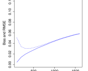
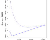
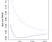
Figure 1: Absolute bias (solid lines) and RMSE (dashed lines) of the M-estimator of $\theta$ as a function of $k$, based on 1 000 samples of size 5 000 from model M1 with parameter values 0.6, 0.75 and 0.9, from left to right.

An analysis of $\widehat{\theta}_{n}$ for a finer range of parameter values is provided in Figure 2. Motivated by the findings in Figure 1 we fix $k=800$; this choice leads to reasonable performance across all parameter values. Overall the results are satisfactory, with a more pronounced negative bias for smaller values of $\theta$ and more variance for increasing $\theta$.

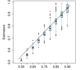
Figure 2: Box plots of the M-Estimators of $\theta$ 1 000 samples of size 5 000 for each parameter value.

5.1.2 The inverted asymmetric logistic model (M2)

Figure 3 shows the impact of $k$ on estimated parameter values for three different choices of $\theta$. Since here the parameter is two-dimensional, we consider (and estimate) the Euclidean bias and RMSE of the estimator $\widehat{\theta}_{n}$, defined as $\|\mathbb{E}[\widehat{\theta}_{n}-\theta]\|$ and $(\mathbb{E}\|\widehat{\theta}_{n}-\theta\|^{2})^{1/2}$, respectively.

Similarly to the pattern observed in Figure 1 we see that smaller values of $\eta$ necessitate larger values of $k$ in order to achieve a good balance between bias and variance.

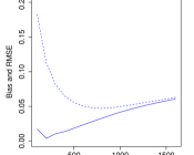
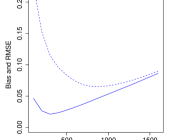
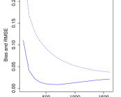
Figure 3: Absolute bias (solid lines) and RMSE (dashed lines) of the M-estimator of $\theta$ as a function of $k$, based on 1 000 samples of size 5 000 from model M2 with parameter $\theta$ equal to $(0.72,0.72)$, $(0.75,0.91)$ and $(0.91,0.91)$, from left to right. In the original parametrization, the corresponding values of $(\nu,\phi)$ are $(0.94,0.94)$, $(0.44,0.94)$ and $(0.31,0.31)$, respectively.

Figure 4 shows the performance of the proposed M-estimator for a range of different parameters $(\theta_{1},\theta_{2})$ with Euclidean bias in the left panel and RMSE in the right panel; the value $k=800$ is fixed throughout. Since the relation $(\nu,\phi)\mapsto(\theta_{1},\theta_{2})$ is not easily invertible, we selected a grid of values of $(\nu,\phi)\in[0,1]^{2}$, calculated all the corresponding points $\theta$ and kept the values for which $\theta_{j}\leq 0.95$, $j=1,2$.

We observe that the estimators perform better for parameter values close to the diagonal, with larger bias and variance for more asymmetric parameter values. The overall estimation accuracy is reasonably good, with worst case RMSE values around 0.07.

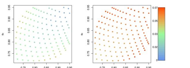
Figure 4: Absolute bias (left) and RMSE (right) of the M-estimator of $\theta=(\theta_{1},\theta_{2})$ as a function of $\theta$, based on 1 000 samples of size 5 000 from model M2.

5.1.3 The Pareto random scale model (M3)

Figure 5 shows the effect of $k$ on the performance of our M-estimator $\widehat{\lambda}_{n}$ in terms of absolute bias and root MSE for the three parameter values $\lambda=0.4$, $1$, and $1.6$. We notice that the estimator is considerably more biased at $\lambda=1$ than at other parameter values. This is expected as, according to Table 1, the bias function $q_{1}$ vanishes only at a logarithmic rate when $\lambda=1$, compared to a polynomial rate elsewhere. Moreover, like in the other models, we observe that for more independent data (characterized by larger $\lambda$), larger values of $k$ are required to drive down the variance of the estimator.

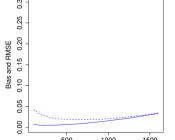
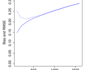
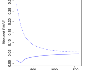
Figure 5: Absolute bias (solid lines) and RMSE (dashed lines) of the M-estimator of $\lambda$ as a function of $k$, based on 1 000 samples of size 5 000 from model M3 with parameter values 0.4, 1 and 1.6, from left to right.

An analysis of $\widehat{\lambda}_{n}$ for a finer range of parameter values is provided in Figure 6. Motivated by Figure 5 we fix $k=400$, which approximately minimizes the maximal RMSE. Overall the estimator is very precise for small values of $\lambda$, but incurs a bias around $\lambda=0.8$ where it struggles to distinguish between values slightly smaller and slightly larger than 1. This phenomenon is not completely unexpected; a close look at Table 1 reveals that $c_{\lambda}$ has almost (but not quite) a symmetry around the point $\lambda=1$, e.g. $c_{0.8}$ is very similar in shape to $c_{1.2}$. This point also corresponds to the transition between asymptotic dependence and independence, which makes estimation challenging.

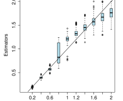
Figure 6: Box plots of the M-Estimators of $\lambda$ based on 1 000 samples of size 5 000 for each parameter value.

5.2 Spatial models

In this section we illustrate the performance of the proposed methodology for spatial data. The candidate class for $c_{\theta}$ results from inverted Brown–Resnick processes with fractal variograms (see Example 6) and takes the form

$$c^{(s)}_{\vartheta}(x,y)=(xy)^{\theta^{(s)}},\quad\theta^{(s)}=\theta(\Delta^{(s)};\vartheta):=\Phi\Big{(}\frac{1}{2}(\Delta^{(s)}/\beta)^{\alpha/2}\Big{)},\quad s\in\mathcal{P},$$ (5.2)

where $\vartheta=(\alpha,\beta)\in(0,2]\times\mathbb{R}_{+}$ and $\Delta^{(s)}$ is the Euclidean distance between the two locations in pair $s$ (measured in units of latitude). Motivated by the data application in the following section, the true parameter values are set as $\vartheta_{0}=(1,3)$ and the values for $\Delta^{(s)}$ are obtained from $40$ randomly sampled pairs of locations in that data set; see Figure S5 in the supplement for a histogram of the distances in this sample.

To evaluate the performance of our estimators we simulate $1000$ independent data sets, each of size $5000$, of an inverted Brown–Resnick process with unit Fréchet margins and fractal variogram from Equation 3.7 with $\alpha=1,\beta=3$. Following the bivariate simulations, to each of the 40 components of the data we add an independent random variable with Pareto distribution function $1-1/x^{4}$, $x\geq 1$. Using the same weight function $g$ as in the bivariate simulations (see Equation 5.1), we compute the two estimators introduced in Equations 3.8 and 3.9. Since the performance of both estimators turns out to be very similar, we only report results for the least squares estimator from Equation 3.8 here and defer all simulations for the estimator (3.9) to Section S6 in the supplement.

Following the discussion in Remark 1, we fix a value $m$ and select each $k^{(s)}$ such that $\widehat{Q}_{n}^{(s)}(k^{(s)}/n,k^{(s)}/n)=m$. The first two panels of Figure 7 show the absolute bias and RMSE of the estimators $\widehat{\alpha}$ and $\widehat{\beta}$, respectively, as functions of $m\in\{75,100,\dots,500\}$. We observe that the RMSE for both estimators is relatively large across all values of $m$. Interestingly, this does not result in a bad performance in estimating the function $\theta(\cdot;\vartheta)$. Indeed, the last panel of Figure 7 shows averaged (over simulation runs) values for $\sup_{0\leq\Delta\leq 3}|\theta(\Delta;\widehat{\vartheta})-\theta(\Delta;\vartheta)|$ and indicates a good overall performance; note that the observed values of $\Delta$ are all smaller than 3 (see Figure S5 in the supplement). This can be explained by the fact that different values of $(\alpha,\beta)$ can lead to somewhat similar curves in the range of interest. This is further illustrated in the left panel of Figure 8 where a random sample of 50 estimated functions $\theta(\Delta;\widehat{\vartheta})$ is displayed.

Figure 7: Left and middle columns: Bias (solid line) and RMSE (dotted line) of the estimators of the two spatial parameters $\alpha$ (left) and $\beta$ (middle) as a function of $m$. Right: Mean of the supremum error $\sup_{0\leq\Delta\leq 3}|\theta(\Delta;\widehat{\alpha},\widehat{\beta})-\theta(\Delta;\alpha,\beta)|$ as a function of $m$.

We conclude this section by fixing $m=150$ and comparing the performance of estimators for $\theta^{(s)}$ based on a bivariate sample at a given distance and the spatial estimator discussed above. Boxplots corresponding to five pairs of stations with distances $\Delta^{(s)}\approx 0.5,1,\dots,2.5$ are shown in the left panel of Figure 8. As expected from the theory, using the spatial estimator is advantageous as it allows to combine information from different distances and leads to a reduced variance.

Figure 8: Left panel: Estimators of $\theta(\Delta)$ for 5 different distances. For each distance, bivariate M-estimator $\widehat{\theta}_{n}^{(s)}$ (green) and spatial estimator $\theta(\Delta^{(s)};\widehat{\alpha},\widehat{\beta})$ (blue) based on the $d=40$ locations. Right panel: 50 sampled curves $\theta(\cdot;\widehat{\alpha},\widehat{\beta})$. Blue represents the true curve $\theta(\cdot;\alpha,\beta)$.

6 Application to rainfall data

In a data set introduced in Le et al. (2018), rainfall was measured daily from 1960 to 2009 at a set of 92 different locations in the state of Victoria, southeastern Australia, for a total of $n=18\,263$ measurements. The conclusions in that paper are that an asymptotically independent model is suitable. A subset of 40 locations, for a total of 780 pairs, was randomly sampled; see the right panel of Figure 9. To the data at those selected locations we fit the same tail model as in Section 5.2, given in Equation 5.2. The weight function $g$ that we use is the same as before and as in Section 5.2, we make use of Remark 1 by fixing a value $m$ and choosing each $k^{(s)}$ accordingly.

We set $m=400$. The left panel of Figure 9 shows the 780 pairwise estimators $\widehat{\theta}_{n}^{(s)}$ plotted against the distances $\Delta^{(s)}$. Despite some estimates at the boundary of the parameter space, the results do not provide much evidence for asymptotic dependence, whereas all estimates are away from the boundary for distances of at least 0.3 units of latitude, strongly suggesting asymptotic independence at these distances. Our two estimators (3.8) and (3.9) of $(\alpha,\beta)$ yield estimates $(\widehat{\alpha},\widehat{\beta})$ of (1.55, 2.24) and (1.56, 2.24), respectively. They are extremely similar, as hinted by the simulation study from Section 5.2. The curve $\theta(\cdot;\widehat{\alpha},\widehat{\beta})$ corresponding to the least squares estimator is also shown in the left panel of Figure 9. The middle panel of Figure 9 displays similar curves for the least squares estimator when $m$ varies from 200 to 1 000. It shows that the estimated curve is robust with respect to the choice of $m$.

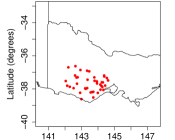
Figure 9: Left: Estimated parameters $\widehat{\theta}_{n}^{(s)}$ against the distances $\Delta^{(s)}$. The black line represents the estimated curve $\theta(\cdot;1.55,2.24)$. Middle: Estimated curve $\theta(\cdot;\widehat{\alpha},\widehat{\beta})$ for the least squares estimator with different values of $m$. Right: The 40 sampled locations in the state of Victoria, southeastern Australia.

S1 Proofs of main results

In this section are collected the proofs of Theorems 1, 2, 3, 4 and 5. A number of more technical results, which are instrumental in the following, are collected in Section S2.

S1.1 Bivariate estimation

For the proofs concerning the bivariate estimators, we assume the framework of Sections 3.1 and 3.2, we define the transformed random variables $U=1-F_{1}(X)$, $V=1-F_{2}(Y)$ and note that $Q$ is the distribution function of the random vector $(U,V)$. Define the transformed observations $U_{i}=1-F_{1}(X_{i})$, $V_{i}=1-F_{2}(Y_{i})$ and denote by $U_{n,1},\dots,U_{n,n}$ and $V_{n,1},\dots,V_{n,n}$ the ordered versions thereof. Additionally define $U_{n,0}=V_{n,0}=0$. For an intermediate sequence $k$, define the random functions $u_{n}$ and $v_{n}$ by

$$u_{n}(x)=\frac{n}{k}U_{n,\lfloor kx\rfloor}\quad\text{and}\quad v_{n}(y)=\frac{n}{k}V_{n,\lfloor ky\rfloor},$$

for $(x,y)\in[0,T]^{2}$. Recalling that $m=nq(k/n)$, it allows us to write

$$\widehat{c}_{n}(x,y)=\frac{n}{m}Q_{n}\left(\frac{k}{n}u_{n}(x),\frac{k}{n}v_{n}(y)\right)$$

where

$$Q_{n}(x,y):=\frac{1}{n}\sum_{i=1}^{n}\mathds{1}\left\{U_{i}\leq x,V_{i}\leq y\right\}$$

denotes the empirical distribution function of $(U_{1},V_{1}),\ldots,(U_{n},V_{n})$. We begin by discussing technical results that will be used in the proof of both Theorem 1 and Theorem 2. Consider the decomposition

$$W_{n}(x,y)= \sqrt{m}\Big{(}\frac{n}{m}Q_{n}\Big{(}\frac{k}{n}u_{n}(x),\frac{k}{n}v_{n}(y)\Big{)}-\frac{n}{m}Q\Big{(}\frac{k}{n}u_{n}(x),\frac{k}{n}v_{n}(y)\Big{)}\Big{)}$$

$$+\sqrt{m}\Big{(}\frac{n}{m}Q\Big{(}\frac{k}{n}u_{n}(x),\frac{k}{n}v_{n}(y)\Big{)}-c(u_{n}(x),v_{n}(y))\Big{)}$$

$$+\sqrt{m}\big{(}c(u_{n}(x),v_{n}(y))-c(x,y)\big{)}.$$

For the second term in the above decomposition, note that

$$\sqrt{m}\Big{(}\frac{n}{m}Q\Big{(}\frac{k}{n}x,\frac{k}{n}y\Big{)}-c(x,y)\Big{)}=O\left(\sqrt{m}q_{1}\left(\frac{k}{n}\right)\right)=o(1)$$

uniformly over all $(x,y)\in[0,2T]^{2}$; here the last equation follows from Condition 1(ii). By Corollary S1 we have $\mathbb{P}(u_{n}(T)\vee v_{n}(T)\leq 2T)\to 1$, and thus

$$\sup_{x,y\in[0,T]}\sqrt{m}\Big{|}\frac{n}{m}Q\Big{(}\frac{k}{n}u_{n}(x),\frac{k}{n}v_{n}(y)\Big{)}-c(u_{n}(x),v_{n}(y))\Big{|}=o_{P}(1).$$

Next define for all $x,y\in[0,2T]$

$$H_{n}(x,y):=\sqrt{m}\Big{(}\frac{n}{m}Q_{n}\Big{(}\frac{k}{n}x,\frac{k}{n}y\Big{)}-\frac{n}{m}Q\Big{(}\frac{k}{n}x,\frac{k}{n}y\Big{)}\Big{)}.$$ (S1.1)

By Lemma S4 this process converges, in $\ell^{\infty}([0,2T]^{2})$, to the process $W$ from Theorem 1 and by Corollary S1 $u_{n}$ and $v_{n}$ converge uniformly in probability to the identity function $I:[0,2T]\to[0,2T]$. Therefore, the triple $(H_{n},u_{n},v_{n})$ converges jointly in distribution to $(W,I,I)$. This implies

$$\sup_{x,y\in[0,T]}\Big{|}H_{n}(u_{n}(x),v_{n}(y))-H_{n}(x,y)\Big{|}=o_{P}(1).$$ (S1.2)

Indeed, consider the map

$$f:\left\{\begin{array}[]{c}\ell^{\infty}([0,2T]^{2})\times\mathcal{V}[0,T]\times\mathcal{V}[0,T]\to\mathbb{R}\\ (a,b_{1},b_{2})\mapsto\sup_{x,y\in[0,T]}|a(b_{1}(x),b_{2}(y))-a(x,y)|\end{array}\right.$$

where $\mathcal{V}[0,T]:=\{g\in\ell^{\infty}[0,T]:g([0,T])\subset[0,2T]\}$ and assume that the product space is equipped with the norm $\|a\|_{\infty}+\|b_{1}\|_{\infty}+\|b_{2}\|_{\infty}$. Observe that $f$ is continuous at points $(a,b_{1},b_{2})$ where $a$ is a continuous function and that the sample paths of $W$ are almost surely continuous. Thus, by the continuous mapping theorem, with probability converging to 1,

$$\sup_{x,y\in[0,T]}\Big{|}H_{n}(u_{n}(x),v_{n}(y))-H_{n}(x,y)\Big{|}=f(H_{n},u_{n},v_{n})\rightsquigarrow f(W,I,I)=0.$$

Since the limit is constant a.s. Equation S1.2 follows. Combining the equations above, we find

$$W_{n}(x,y)=H_{n}(x,y)+\sqrt{m}\big{(}c(u_{n}(x),v_{n}(y))-c(x,y)\big{)}+o_{P}(1),$$ (S1.3)

where the term $o_{P}(1)$ is uniform on $[0,T]^{2}$, and we recall that $H_{n}\rightsquigarrow W$ in $\ell^{\infty}([0,2T]^{2})$.

S1.1.1 Proof of Theorem 1

Define

$$S_{n}(x,y):=\sqrt{m}\big{(}c(u_{n}(x),v_{n}(y))+c(x,y)\big{)}.$$

In light of Equation S1.3 it suffices to prove that $S_{n}\stackrel{{\scriptstyle P}}{{\to}}0$ uniformly on $[0,T]^{2}$. From here on it is more convenient to study component-wise increments. That is, we write

$$S_{n}(x,y) =\sqrt{m}(c(u_{n}(x),y)-c(x,y))+\sqrt{m}(c(u_{n}(x),v_{n}(y))-c(u_{n}(x),y))$$

$$=:S_{n}^{(a)}(x,y)+S_{n}^{(b)}(x,y)$$

and we will show that both $S_{n}^{(a)}$ and $S_{n}^{(b)}$ converge to 0 in probability, starting with $S_{n}^{(a)}$.

By assumption, since with probability converging to 1 we have $u_{n}(x)\in[0,2T]$ for every $x\leq T$, we can write

$$S_{n}^{(a)}(x,y) =\sqrt{m}\left(c(u_{n}(x),y)+c(x,y)\right)$$ (S1.4)

$$=\sqrt{m}\left\{\frac{n}{m}Q\left(\frac{k}{n}u_{n}(x),\frac{k}{n}y\right)-\frac{n}{m}Q\left(\frac{k}{n}x,\frac{k}{n}y\right)+O_{P}\left(q_{1}\left(\frac{k}{n}\right)\right)\right\}$$

$$=\frac{n}{\sqrt{m}}\left(Q\left(\frac{k}{n}u_{n}(x),\frac{k}{n}y\right)-Q\left(\frac{k}{n}x,\frac{k}{n}y\right)\right)+o_{P}\left(1\right)$$ (S1.5)

uniformly on $[0,T]^{2}$, since the sequence $m$ was chosen so that $\sqrt{m}q_{1}(k/n)\to 0$. We will use both Equations S1.4 and S1.5 as representations of $S_{n}^{(a)}$ throughout the proof.

Let $\beta_{n}=(m/k)/(\log(k/m))$. From there, partition $[0,T]^{2}$ in $\Theta_{n}^{(1)}=[0,1/k)\times[0,T]$, $\Theta_{n}^{(2)}=[1/k,\beta_{n})\times[0,T]$ and $\Theta_{n}^{(3)}=[\beta_{n},T]\times[0,T]$ (if $\beta_{n}<1/k$, $\Theta_{n}^{(2)}$ is empty). These sets represent the “small”, “intermediate” and “large” values of $x$, respectively. We will prove that the suprema of $S_{n}^{(a)}$ on $\Theta_{n}^{(1)}$, $\Theta_{n}^{(2)}$ and $\Theta_{n}^{(3)}$ all converge to 0 in probability. Equation S1.5 yields

$$\sup_{(x,y)\in\Theta_{n}^{(1)}}|S_{n}^{(a)}(x,y)| =\frac{n}{\sqrt{m}}\sup_{0\leq x<1/k}\left|Q\left(\frac{k}{n}u_{n}(x),\frac{k}{n}y\right)-Q\left(\frac{k}{n}x,\frac{k}{n}y\right)\right|+o_{P}(1)$$

$$=\frac{n}{\sqrt{m}}\sup_{0\leq x<1/k}Q\left(\frac{k}{n}x,\frac{k}{n}y\right)+o_{P}(1)$$

$$\leq\frac{n}{\sqrt{m}}\frac{1}{n}+o_{P}(1)$$

$$=\frac{1}{\sqrt{m}}+o_{P}(1),$$

where we have once again used the facts that $u_{n}(x)=0$ whenever $x<1/k$ and that $Q(0,\cdot)=Q(\cdot,0)=0$, in addition to the fact that $Q(u,v)\leq u$. This proves that $\sup_{\Theta_{n}^{(1)}}|S_{n}^{(a)}|\to 0$ in probability.

Using Equation S1.5 again, the supremum of $S_{n}^{(a)}$ on $\Theta_{n}^{(2)}$ can be expressed as

$$\sup_{1/k\leq x<\beta_{n}}\left|S_{n}^{(a)}(x,y)\right| =\sup_{1/k\leq x<\beta_{n}}\frac{n}{\sqrt{m}}\left|Q\left(\frac{k}{n}u_{n}(x),\frac{k}{n}y\right)-Q\left(\frac{k}{n}x,\frac{k}{n}y\right)\right|+o_{P}\left(1\right)$$

$$\leq\sup_{1/k\leq x<\beta_{n}}\frac{n}{\sqrt{m}}\left|\frac{k}{n}u_{n}(x)-\frac{k}{n}x\right|+o_{P}\left(1\right)$$

$$=\sup_{1/k\leq x<\beta_{n}}\frac{k}{\sqrt{m}}|u_{n}(x)-x|+o_{P}\left(1\right)$$

$$=O_{P}\left(\sup_{1/k\leq x<\beta_{n}}\sqrt{\frac{k}{m}}\varphi(x)\right)+o_{P}\left(1\right),$$

where we have used Lipschitz continuity of $Q$ and Lemma S3. The last bound holds for any function $\varphi$ that satisfies the conditions in Lemma S3, but from now on we use $\varphi(x):=\sqrt{x\log\log(1/x)}$ on $(0,B]$ and $\varphi(x):=\sqrt{x}$ on $(B,T]$, where $B>0$ is chosen small enough so that $\varphi$ is well defined and non-decreasing. By monotonicity, the supremum is attained at $x=\beta_{n}$. We then have

$$\sup_{1/k\leq x<\beta_{n}}\left|S_{n}^{(a)}(x,y)\right|=O_{P}\left(\sqrt{\frac{k}{m}\beta_{n}\log\log(1/\beta_{n})}\right)+o_{P}\left(1\right)$$

because since $\beta_{n}\to 0$, eventually $\beta_{n}\leq B$, so eventually $\varphi(\beta_{n})=\sqrt{\beta_{n}\log\log(1/\beta_{n})}$. The last display converges in probability to 0 since

$$\frac{k}{m}\beta_{n}\log\log(1/\beta_{n})=\frac{\log\log\left(\frac{k}{m}\log(k/m)\right)}{\log(k/m)}\longrightarrow 0$$

as $k/m\to\infty$, which proves that $\sup_{\Theta_{n}^{(2)}}|S_{n}^{(a)}|\to 0$ in probability.

Finally, when considering large values of $x$, Lemma S3 and a combination of Equations S2.7 and S7 imply that

$$\sup_{\beta_{n}\leq x\leq T}\left|S_{n}^{(a)}(x,y)\right| =\sup_{\beta_{n}\leq x\leq T}\sqrt{m}|c(u_{n}(x),y)-c(x,y)|$$

$$\lesssim\sqrt{m}\sup_{\beta_{n}\leq x\leq T}|u_{n}(x)-x|r(x\vee u_{n}(x))$$

$$=O_{P}\left(\sqrt{\frac{m}{k}}\sup_{\beta_{n}\leq x\leq T}\varphi(x)r(x\vee u_{n}(x))\right),$$

where $r(x)=(x\log(1/x))^{-1}$. By monotonicity of $\varphi$, the inside of the $O_{P}$ can be upper bounded by

$$\sqrt{\frac{m}{k}}\sup_{\beta_{n}\leq x\leq T}\varphi(x\vee u_{n}(x))r(x\vee u_{n}(x))$$

and since with probability converging to 1, for every $x\leq T$, $u_{n}(x)\leq 2T$, this can in turn be upper bounded (with probability converging to 1) by

$$\sqrt{\frac{m}{k}}\sup_{\beta_{n}\leq x\leq 2T}\varphi(x)r(x).$$

It can easily be checked (e.g. by differentiation) that the function $\varphi\times r$ is decreasing. Thus, the above supremum is attained at $\beta_{n}$. Finally, elementary computations yield

$$\sqrt{\frac{m}{k}}\varphi(\beta_{n})r(\beta_{n})\lesssim\sqrt{\frac{\log\log((k/m)^{2})}{\log(k/m)}}\longrightarrow 0.$$

Overall, we have shown that $S_{n}^{(a)}\stackrel{{\scriptstyle P}}{{\to}}0$ uniformly over $[0,T]^{2}$. Note that all the bounds we derived are uniform over all values of $y\in[0,T]$, although it was removed from the notation for parsimony. In order to deal with $S_{n}^{(b)}$, we recall once again that with probability converging to 1, we have $u_{n}(x)\leq 2T$ for every $x\leq T$. Therefore, with probability converging to 1,

$$\sup_{(x,y)\in[0,T]^{2}}\left|S_{n}^{(b)}(x,y)\right| =\sup_{(x,y)\in[0,T]^{2}}\sqrt{m}|c(u_{n}(x),v_{n}(y))-c(u_{n}(x),y)|$$

$$\leq\sup_{x\in[0,2T],y\in[0,T]}\sqrt{m}|c(x,v_{n}(y))-c(x,y)|.$$

This can be shown to converge in probability to 0 using the exact same proof as for $S_{n}^{(a)}$. We finally conclude that $S_{n}\stackrel{{\scriptstyle P}}{{\to}}0$ in $\ell^{\infty}([0,T]^{2})$, and the proof for deterministic $k=k_{n}$ is complete. It remains to show that the result continues to hold if we replace the deterministic sequence $k=k_{n}$ by data-dependent $\widehat{k}$ as outlined in Remark 1. This is established in Section S1.1.3. $\square$

S1.1.2 Proof of Theorem 2

In view of Equation S1.3, we require the joint asymptotic behavior of $H_{n}$, $u_{n}$ and $v_{n}$. Define, for $(x,y)\in[0,\infty)^{2}$,

$$L_{n}^{(1)}(x)=\frac{1}{k}\sum_{i=1}^{n}\mathds{1}\left\{U_{i}\leq\frac{k}{n}x\right\}\quad\text{and}\quad L_{n}^{(2)}(y)=\frac{1}{k}\sum_{i=1}^{n}\mathds{1}\left\{V_{i}\leq\frac{k}{n}y\right\},$$

a rescaled version of the marginal empirical distribution functions of $U$ and $V$. We now show that the $\mathbb{D}$-valued process

$$(x,y)\mapsto\left(H_{n}(x,y),\sqrt{m}\left(L_{n}^{(1)}(x)-x\right),\sqrt{m}\left(L_{n}^{(2)}(y)-y\right)\right)$$ (S1.6)

converges in distribution to the Gaussian process $(W,W^{(1)},W^{(2)})$ defined in Section 4.1.1 with covariance matrix $\Lambda$ from Equation 4.2, where $\mathbb{D}:=\big{(}\ell^{\infty}([0,2T]^{2})\big{)}^{3}$.

Again, let $I$ denote the identity map on $\mathbb{R}$. The three processes $H_{n}$, $\sqrt{m}(L_{n}^{(1)}-I)$ and $\sqrt{m}(L_{n}^{(2)}-I)$ are individually tight (see Lemma S4) and hence it suffices to prove convergence of the marginal distributions. This in turn follows from convergence of the covariance function, by the multivariate Lindeberg-Feller theorem (see van der Vaart (2000), Theorem 2.27); verification of the Lindeberg condition is similar to condition (B) in the proof of Lemma S4. The convergence of $\mathbb{E}\left[H_{n}(x,y)H_{n}(x^{\prime},y^{\prime})\right]$ to $c(x\wedge x^{\prime},y\wedge y^{\prime})$ is already shown in Lemma S4. Using similar arguments and recalling that $m/k\to\chi>0$, one easily deals with the other covariance terms and concludes that the processes in Equation S1.6 weakly converge to $(W,W^{(1)},W^{(2)})$ in $\mathbb{D}$.

Note that the random functions $u_{n}$ and $v_{n}$ are the generalized inverses of $L_{n}^{(1)}+1/k$ and $L_{n}^{(2)}+1/k$, respectively. Because $\sqrt{m}/k\to 0$, the term $1/k$ is negligible. Upon applying Vervaat’s lemma (Vervaat (1972)), which states that the generalized inverse mapping is Hadamard differentiable around the identity function, we deduce that the processes $G_{n}$, defined by

$$G_{n}(x,y)=(H_{n}(x,y),\sqrt{m}(u_{n}(x)-x),\sqrt{m}(v_{n}(y)-y)),$$

weakly converge to $(W,-W^{(1)},-W^{(2)})$ in $\mathbb{D}$. For $t>0$, define the sets

$$\mathcal{V}(t):=\{b\in\ell^{\infty}([0,2T]):\forall x\in[0,T],x+tb(x)\in[0,2T]\}.$$ (S1.7)

Let $\mathbb{D}_{n}\subset\mathbb{D}$ be the subset of functions $a=(a^{(0)},a^{(1)},a^{(2)})$ such that $a^{(1)}(x,y)$ is constant in $y$, $a^{(2)}(x,y)$ is constant in $x$ and the functions $x\mapsto a^{(1)}(x,y)$ and $y\mapsto a^{(2)}(x,y)$ are elements of $\mathcal{V}(1/\sqrt{m})$. Let $\mathbb{E}$ be the space of equivalence classes $L^{\infty}([0,T]^{2})$ equipped with the topology of hypi-convergence. Define the functionals $f_{n}:\mathbb{D}_{n}\to\mathbb{E}$ by

$$f_{n}(a)(x,y):=a^{(0)}(x,y)+\sqrt{m}\left(c\left(x+\frac{a^{(1)}(x,y)}{\sqrt{m}},y+\frac{a^{(2)}(x,y)}{\sqrt{m}}\right)-c(x,y)\right).$$

Equation S1.3 can be rephrased as $W_{n}=f_{n}(G_{n})+o_{P}\left(1\right)$, assuming that $G_{n}\in\mathbb{D}_{n}$, which is true with probability

$$\mathbb{P}\left(u_{n}(T)\leq 2T,v_{n}(T)\leq 2T\right)\longrightarrow 1.$$

Let $\mathbb{D}_{0}\subset\mathbb{D}$ be the subset of continuous functions $a$ such that $a(0)=0$. As soon as $a_{n}\in\mathbb{D}_{n}$ converges uniformly to $a\in\mathbb{D}_{0}$, by Lemma S9, $f_{n}(a_{n})$ hypi-converges to $f(a)$, where $f:\mathbb{D}_{0}\to\mathbb{E}$ satisfies

$$f(a):=a^{(0)}+\dot{c}_{1}a^{(1)}+\dot{c}_{2}a^{(2)}.$$

Note that $(W,-W^{(1)},-W^{(2)})$ concentrates on $\mathbb{D}_{0}$. Therefore, by the extended continuous mapping theorem (van der Vaart and Wellner, 1996, Theorem 1.11.1),

$$W_{n}=f_{n}(G_{n})+o_{P}\left(1\right)\rightsquigarrow f((W,-W^{(1)},-W^{(2)}))=W-\dot{c}_{1}W^{(1)}-\dot{c}_{2}W^{(2)}$$

in $\mathbb{E}$. It remains to show that the result continues to hold if we replace the deterministic sequence $k=k_{n}$ by data-dependent $\widehat{k}$ as outlined in Remark 1. This is established in Section S1.1.3. $\square$

S1.1.3 Proof that Theorems 1 and 2 continue to hold with $\widehat{k}$

Let $\widehat{c}_{n,\widehat{k}}$ be the estimator $\widehat{c}_{n}$ computed with the random quantity $\widehat{k}$ instead of $k$. We shall prove that $\sqrt{m}|\widehat{c}_{n,\widehat{k}}-\widehat{c}_{n}|\to 0$ in probability uniformly over $[0,T]^{2}$ (under asymptotic independence) or in the hypi semimetric (under asymptotic dependence).

Note that the definition of $\widehat{k}$ implies that $\widehat{c}_{n}(\widehat{k}/k,\widehat{k}/k)=1$. By assumption, $\widehat{c}_{n}$ converges to $c$ in probability uniformly in a neighborhood of $(1,1)$. Jointly with the fact that $c(x,x)=x^{1/\eta}$, this readily implies that $\widehat{k}/k\to 1$ in probability. Further note that

$$\widehat{c}_{n,\widehat{k}}(x,y)=\frac{q(k/n)}{q(\widehat{k}/n)}\widehat{c}_{n}(\widehat{k}x/k,\widehat{k}y/k).$$

We first discuss the case of asymptotic independence. By Theorem 1 and by Skorokhod’s almost sure representation, we may assume that almost surely, $\widehat{c}_{n}=c+W/\sqrt{m}+{o(1/\sqrt{m})}$ and $\widehat{k}/k\to 1$. The object of interest is then equal, with probability one, to

$$\frac{q(k/n)}{q(\widehat{k}/n)}\sqrt{m}\left(\widehat{c}_{n}(\widehat{k}x/k,\widehat{k}y/k)-\frac{q(\widehat{k}/n)}{q(k/n)}\widehat{c}_{n}(x,y)\right)$$

$$\quad={\frac{q(k/n)}{q(\widehat{k}/n)}}\Big{\{}\sqrt{m}\Big{(}c(\widehat{k}x/k,\widehat{k}y/k)-\frac{q(\widehat{k}/n)}{q(k/n)}c(x,y)\Big{)}+W(\widehat{k}x/k,\widehat{k}y/k)-W(x,y)\Big{\}}+o(1)$$

$$\quad=-\sqrt{m}c(x,y)\left(\frac{q(\widehat{k}/n)}{q(k/n)}-\bigg{(}\frac{\widehat{k}/n}{k/n}\bigg{)}^{1/\eta}\right){\frac{q(k/n)}{q(\widehat{k}/n)}}+o(1),$$ (S1.8)

where we have used homogeneity of $c$, regular variation of $q$ and the fact that almost surely, the sample paths of $W$ are continuous, hence uniformly continuous on compact sets. The terms $o(1)$ are uniform over $[0,T]^{2}$. Finally, it is shown in Lemma S2 that uniformly over $a$ in a neighborhood of 1, $q(at)/q(t)-a^{1/\eta}=O(q_{1}(t))$. Recalling that $\widehat{k}/k\to 1$ almost surely, the first term in Equation S1.8 is then uniformly of the order of $\sqrt{m}q_{1}(k/n)$, which vanishes by Condition 1(ii).

In the case of asymptotic dependence, Theorem 2 ensures that $\widehat{c}_{n}=c+B/\sqrt{m}+o(1/\sqrt{m})$ in the hypi semimetric. We may apply the reasoning above except that, from the definition of the process $B$, we get the additional term

$$-\sum_{j=1}^{2}\Big{(}\dot{c}_{j}(\widehat{k}x/k,\widehat{k}y/k)W^{(j)}(\widehat{k}x/k,\widehat{k}y/k)-\dot{c}_{j}(x,y)W^{(j)}(x,y)\Big{)}\\ =-\sum_{j=1}^{2}\dot{c}_{j}(x,y)\Big{(}W^{(j)}(\widehat{k}x/k,\widehat{k}y/k)-W^{(j)}(x,y)\Big{)};$$ (S1.9)

this follows from the fact that under asymptotic dependence, $c$ is homogeneous of order 1 and the directional partial derivatives of such a function, when they exist, are constant along rays from the origin. The above term vanishes uniformly since $\dot{c}_{j}$ has to be locally bounded (only under asymptotic dependence) and since the sample paths of $W^{(j)}$ are almost surely continuous. We therefore obtain Equation S1.8, except that this time the term $o(1)$ is understood in the hypi semimetric. From here on the proof is completed in the same way as under asymptotic independence. $\square$

S1.1.4 Proof of Theorem 3

Recall the definition of $\Psi_{n}$ from Section 3.2. Letting $\widehat{\sigma}_{n}=\frac{n}{m}\widehat{\zeta}_{n}$, the assumption that $(\widehat{\theta}_{n},\widehat{\zeta}_{n})$ minimizes the norm of $\Psi_{n}^{*}$ becomes equivalent to $(\widehat{\theta}_{n},\widehat{\sigma}_{n})$ minimizing the norm of $\Psi_{n}$. The key is to note that for any $\theta,\sigma$,

$$\Psi(\theta,\sigma)-\Psi_{n}(\theta,\sigma)=\int g(\widehat{c}_{n}-c)d\mu_{\text{L}}=\frac{1}{\sqrt{m}}\int gW_{n}d\mu_{\text{L}},$$ (S1.10)

with $W_{n}$ defined as in Theorems 1 and 2. By the dominated convergence theorem, and because $g$ is integrable, one easily sees that the functional $f\mapsto\int gfd\mu_{\text{L}}$ is continuous in $\ell^{\infty}([0,T]^{2})$. By Lemma S10, this is also true in the topology of hypi-convergence on $\ell^{\infty}([0,T]^{2})$ at points $f$ that are continuous Lebesgue-almost everywhere on $[0,T]^{2}$. It is the case of both limiting Gaussian processes appearing in Theorems 1 and 2: $W$, $W^{(1)}$ and $W^{(2)}$ have almost surely continuous sample paths and under asymptotic dependence, the directional derivatives $\dot{c}_{j}$ are almost everywhere continuous. Those two results and the continuous mapping theorem then imply that

$$\int gW_{n}d\mu_{\text{L}}\rightsquigarrow N(0,A).$$

We may therefore apply Lemma S11 with $\phi=\Psi$, $x_{0}=(\theta_{0},1)$, $Y_{n}=\frac{1}{\sqrt{m}}\int gW_{n}d\mu_{\text{L}}$ and $a_{n}=1/\sqrt{m}$, and as required we obtain

$$\sqrt{m}((\widehat{\theta}_{n},\widehat{\sigma}_{n})-(\theta_{0},1))=(J^{\top}J)^{-1}J^{\top}\int gW_{n}d\mu_{\text{L}}+o_{P}\left(1\right)\rightsquigarrow N(0,\Sigma).$$

$\square$

S1.2 Spatial estimation

For the proofs in the spatial setting, we assume the framework of Section 3.3, we define the transformed random variables $U^{(j)}=1-F^{(j)}(X^{(j)})$ and for a pair $s$, let $Q^{(s)}$ be the distribution function of the random vector $(U^{(s_{1})},U^{(s_{2})})$. Define the transformed observations $U_{i}^{(j)}=1-F^{(j)}(X_{i}^{(j)})$ and denote by $U_{n,1}^{(j)},\dots,U_{n,n}^{(j)}$ the ordered versions thereof and define $U_{n,0}^{(j)}:=0$. For intermediate sequences $k^{(s)}$, we define the (weighted) empirical tail quantile functions $u_{n}^{(s,j)}$, $s\in\mathcal{P},j\in\{1,2\}$, by

$$u_{n}^{(s,j)}(x)=\frac{n}{k^{(s)}}U_{n,\lfloor k^{(s)}x\rfloor}^{(s_{j})},\quad x\geq 0.$$

Recalling that $m^{(s)}=nq^{(s)}(k^{(s)}/n)$, it allows us to write

$$\widehat{c}_{n}^{(s)}(x,y)=\frac{n}{m^{(s)}}Q_{n}^{(s)}\left(\frac{k^{(s)}}{n}u_{n}^{(s,1)}(x),\frac{k^{(s)}}{n}u_{n}^{(s,2)}(y)\right).$$

where $Q_{n}^{(s)}$ denotes the empirical distribution function of $(U_{1}^{(s_{1})},U_{1}^{(s_{2})}),\ldots,(U_{n}^{(s_{1})},U_{n}^{(s_{2})})$. Following the discussion before the proof of Theorem 1, we may define

$$H_{n}^{(s)}(x,y):=\sqrt{m^{(s)}}\Big{\{}\frac{1}{m^{(s)}}\sum_{i=1}^{n}\mathbb{I}\Big{\{}U_{i}^{(s_{1})}\leq\frac{k^{(s)}}{n}x,U_{i}^{(s_{2})}\leq\frac{k^{(s)}}{n}y\Big{\}}\\ -\frac{n}{m^{(s)}}\mathbb{P}\Big{(}{U^{(s_{1})}\leq\frac{k^{(s)}}{n}x,U^{(s_{2})}\leq\frac{k^{(s)}}{n}y}\Big{)}\Big{\}}.$$

and similarly obtain

$$W_{n}^{(s)}(x,y)=H_{n}^{(s)}(x,y)+\sqrt{m^{(s)}}\left(c^{(s)}\left(u_{n}^{(s,1)}(x),u_{n}^{(s,2)}(y)\right)-c^{(s)}(x,y)\right)+o_{P}\left(1\right),$$ (S1.11)

where $W_{n}^{(s)}$ is defined as in Theorem 4 and the term $o_{P}\left(1\right)$ is uniform over compact sets.

S1.2.1 Proof of Theorem 4

For asymptotically independent pairs, the second term of Equation S1.11 vanishes uniformly, by the proof of Theorem 1. Define the $\mathbb{D}$-valued processes $G_{n}$ by

$$G_{n}(x,y):=\left(\left(H_{n}^{(s)}(x,y)\right)_{s\in\mathcal{P}},\left(\sqrt{m^{(s)}}\left(u_{n}^{(s,1)}(x)-x\right),\sqrt{m^{(s)}}\left(u_{n}^{(s,2)}(y)-y\right)\right)_{s\in\mathcal{P}_{D}}\right),$$

where $\mathbb{D}=\left(\ell^{\infty}([0,2T]^{2})\right)^{|\mathcal{P}|+2|\mathcal{P}_{D}|}$. The proof now proceeds similarly to that of Theorem 2; we show that $G_{n}$ converges in distribution, that the processes of interest $W_{n}^{(s)}$ can be approximately represented as a transformation of $G_{n}$, and we conclude by applying a continuous mapping theorem.

For $s\in\mathcal{P}$, $j\in\{1,2\}$, let

$$L_{n}^{(s,j)}(x)=\frac{1}{k^{(s)}}\sum_{i=1}^{n}\mathds{1}\left\{U^{(s_{j})}\leq\frac{k^{(s)}}{n}x\right\},\quad x\geq 0.$$

Recall that $I$ denotes the identity mapping on $\mathbb{R}$. By standard arguments (see, e.g., the proofs of Theorems 1 and 2), we see that each of the processes $H_{n}^{(s)}$ and $\sqrt{m^{(s)}}\left(L_{n}^{(s,j)}-I\right)$ converge in distribution in $\ell^{\infty}([0,2T]^{2})$, hence they are tight random elements in that space. It follows that the sequence of processes

$$(x,y)\mapsto\left(\left(H_{n}^{(s)}(x,y)\right)_{s\in\mathcal{P}},\left(\sqrt{m^{(s)}}\left(L_{n}^{(s,1)}(x)-x\right),\sqrt{m^{(s)}}\left(L_{n}^{(s,2)}(y)-y\right)\right)_{s\in\mathcal{P}_{D}}\right)$$ (S1.12)

is tight in the product space $\mathbb{D}$. A Lindeberg-type condition (van der Vaart, 2000, Theorem 2.27) can easily be checked, so weak convergence of the process in Equation S1.12 follows from convergence of $\mathbb{E}\left[G_{n}(x,y)G_{n}(x^{\prime},y^{\prime})^{\top}\right]$ to a suitable covariance matrix. This is simply a consequence of Condition 2; indeed, for suitable pairs $s,s^{\prime}\in\mathcal{P}$, $j,j^{\prime}\in\{1,2\}$ and $(x,y),(x^{\prime},y^{\prime})\in[0,\infty)^{2}$, this condition implies that

$$\lim_{n\to\infty}\mathbb{E}\left[H_{n}^{(s)}(x,y)H_{n}^{(s^{\prime})}(x^{\prime},y^{\prime})\right] =\Gamma^{(s,s^{\prime})}((x,y),(x^{\prime},y^{\prime})),$$

$$\lim_{n\to\infty}\mathbb{E}\left[H_{n}^{(s)}(x,y)\sqrt{m^{(s^{\prime})}}\left(L_{n}^{(s^{\prime},j)}(x^{\prime})-x^{\prime}\right)\right] =\Gamma^{(s,s^{\prime},j)}((x,y),(x^{\prime},y^{\prime})),$$

$$\lim_{n\to\infty}\mathbb{E}\left[\sqrt{m^{(s)}}\left(L_{n}^{(s,j)}(x)-x\right)\sqrt{m^{(s^{\prime})}}\left(L_{n}^{(s^{\prime},j^{\prime})}(x^{\prime})-x^{\prime}\right)\right] =\Gamma^{(s,j,s^{\prime},j^{\prime})}((x,y),(x^{\prime},y^{\prime})).$$

We deduce that in $\mathbb{D}$, the processes in Equation S1.12 weakly converge to the Gaussian process

$$\left((W^{(s)})_{s\in\mathcal{P}},(W^{(s,j)})_{s\in\mathcal{P}_{D},j\in\{1,2\}}\right)$$

as defined in Section 4.2. Noting that $u_{n}^{(s,j)}$ is the generalized inverse function of $L_{n}^{(s,j)}+1/k^{(s)}$ and that $\sqrt{m^{(s)}}/k^{(s)}\to 0$, we apply Vervaat’s lemma (Vervaat, 1972) to obtain that

$$G_{n}\rightsquigarrow G:=\left((W^{(s)})_{s\in\mathcal{P}},(-W^{(s,j)})_{s\in\mathcal{P}_{D},j\in\{1,2\}}\right)$$ (S1.13)

in $\mathbb{D}$.

Recall the definition of the sets $\mathcal{V}(t)$ in Equation S1.7 and let $\mathbb{D}_{n}\subset\mathbb{D}$ be the subset of functions $a$ of the form $\big{(}(a^{(s)})_{s\in\mathcal{P}},(a^{(s,j)})_{s\in\mathcal{P}_{D},j\in\{1,2\}}\big{)}$ such that $a^{(s,1)}(x,y)$ is constant in $y$, $a^{(s,2)}(x,y)$ is constant in $x$ and such that the functions $x\mapsto a^{(s,1)}(x,y)$ and $y\mapsto a^{(s,2)}(x,y)$ are elements of $\mathcal{V}\big{(}1/\sqrt{m^{(s)}}\big{)}$.

Defining $\mathbb{E}$ as the product space $\left(L^{\infty}([0,T]^{2})\right)^{|\mathcal{P}|}$, with $L^{\infty}([0,T]^{2})$ equipped with the topology of hypi-convergence, consider the following functionals $f_{n}:\mathbb{D}_{n}\to\mathbb{E}$. For an element $a=\big{(}(a^{(s)})_{s\in\mathcal{P}},(a^{(s,j)})_{s\in\mathcal{P}_{D},j\in\{1,2\}}\big{)}\in\mathbb{D}_{n}$, $f_{n}(a)=(f_{n}(a)^{(s)})_{s\in\mathcal{P}}$ is a function such that $f_{n}(a)^{(s)}=a^{(s)}$ if $s\in\mathcal{P}_{I}$, and

$$f_{n}(a)^{(s)}(x,y)=a^{(s)}(x,y)+\sqrt{m^{(s)}}\left(c^{(s)}\left(x+\frac{a^{(s,1)}(x,y)}{\sqrt{m^{(s)}}},y+\frac{a^{(s,2)}(x,y)}{\sqrt{m^{(s)}}}\right)-c^{(s)}(x,y)\right)$$

if $s\in\mathcal{P}_{D}$. Referring to Equation S1.11 and recalling that the second term thereof vanishes if $s\in\mathcal{P}_{I}$, we notice that for every pair $s$, $W_{n}^{(s)}=f_{n}(G_{n})^{(s)}+o_{P}\left(1\right)$. This representation, of course, holds only if $G_{n}\in\mathbb{D}_{n}$; this is satisfied with probability at least

$$\mathbb{P}\left(\forall s\in\mathcal{P}_{D},j\in\{1,2\},u_{n}^{(s,j)}(T)\leq 2T\right)\longrightarrow 1$$

where the last convergence follows by Corollary S1 applied for each $s\in\mathcal{P}$. Define $f:\mathbb{D}_{0}\to\mathbb{E}$, where $\mathbb{D}_{0}\subset\mathbb{D}$ is the subset of continuous functions $a$ such that $a(0)=0$, as

$$f(a)^{(s)}=\begin{cases}a^{(s)},&\quad s\in\mathcal{P}_{I}\\ a^{(s)}+\dot{c}_{1}a^{(s,1)}+\dot{c}_{2}a^{(s,2)},&\quad s\in\mathcal{P}_{D}\end{cases}.$$

For a sequence $a_{n}\in\mathbb{D}_{n}$ that converges uniformly to a function $a\in\mathbb{D}_{0}$, $f_{n}(a_{n})\to f(a)$ in $\mathbb{E}$. This can be seen by considering each pair separately; the result is obvious for asymptotically independent pairs, and for asymptotically dependent ones it follows from Lemma S9.

Finally, notice that the process $G$ concentrates on $\mathbb{D}_{0}$. Therefore, by Equation S1.13 and the extended continuous mapping theorem (van der Vaart and Wellner, 1996, Theorem 1.11.1),

$$\Big{(}W_{n}^{(s)}\Big{)}_{s\in\mathcal{P}}=f_{n}(G_{n})+o_{P}\left(1\right)\rightsquigarrow f(G)=\Big{(}B^{(s)}\Big{)}_{s\in\mathcal{P}}$$

in $\mathbb{E}$. $\square$

S1.2.2 Proof of Theorem 5

Similarly to the bivariate case, let

$$\Psi_{n}^{(s)}(\theta,\sigma):=(n/m)\Psi_{n}^{*(s)}(\theta,m\sigma/n).$$

As in the proof of Theorem 3, we may deduce that for every pair $s$, $\theta\in\widetilde{\Theta}$ and $\sigma>0$,

$$\Psi^{(s)}(\theta,\sigma)-\Psi_{n}^{(s)}(\theta,\sigma)=\int g\left(\widehat{c}_{n}^{(s)}-c^{(s)}\right)d\mu_{\text{L}}=\frac{1}{\sqrt{m}}\int gW_{n}^{(s)}d\mu_{\text{L}},$$

with $W_{n}^{(s)}$ as defined in Theorem 4. By a similar argument to the bivariate case (involving the dominated convergence theorem and Lemma S10 to establish continuity of the mapping $f\mapsto\int gfd\mu_{\text{L}}$, see the proof of Theorem 3 for the applicability of Lemma S10), Theorem 4 and the continuous mapping theorem yield

$$\left(\int gW_{n}^{(s)}d\mu_{\text{L}}\right)_{s\in\mathcal{P}}\rightsquigarrow\left(\int gB^{(s)}d\mu_{\text{L}}\right)_{s\in\mathcal{P}}.$$ (S1.14)

The remaining proof consists of a number of successive applications of Lemma S11. We deal with each of the two estimators separately.

• For each pair $s$, applying Lemma S11 with $\phi=\Psi^{(s)}$, $x_{0}=(h^{(s)}(\vartheta_{0}),1)$, $a_{n}=1/\sqrt{m}$ and $Y_{n}=\frac{1}{\sqrt{m}}\int gW_{n}^{(s)}d\mu_{\text{L}}$ yields

  $$\widehat{\theta}_{n}^{(s)}-h^{(s)}(\vartheta_{0})=\frac{1}{\sqrt{m}}\mathcal{D}^{(s)}\int gW_{n}^{(s)}d\mu_{\text{L}}+o_{P}\left(\frac{1}{\sqrt{m}}\right),$$ (S1.15)

  where $\mathcal{D}^{(s)}$ is the block corresponding to the pair $s$ in the matrix $\mathcal{D}$ defined in Equation 4.4; its existence, as well as the required smoothness of $\phi$, are guaranteed by Condition 3. Now redefining $\phi$ as $\phi(\vartheta)=\big{(}h^{(s)}(\vartheta)-h^{(s)}(\vartheta_{0})\big{)}_{s\in\mathcal{P}}$, we see that $\widehat{\vartheta}_{n}$ is in fact a minimizer of the norm of $\phi(\vartheta)-Y_{n}$, where $Y_{n}$ is redefined as $\big{(}\widehat{\theta}_{n}^{(s)}-h^{(s)}(\vartheta_{0})\big{)}_{s\in\mathcal{P}}$. Applying Lemma S11 again with $\phi$ and $Y_{n}$ as above, $x_{0}=\vartheta_{0}$ and $a_{n}=1/\sqrt{m}$, we obtain

  $$\widehat{\vartheta}_{n}-\vartheta_{0} =(J_{1}^{\top}J_{1})^{-1}J_{1}^{\top}Y_{n}+o_{P}\left(\frac{1}{\sqrt{m}}\right)$$

  $$=\frac{1}{\sqrt{m}}(J_{1}^{\top}J_{1})^{-1}J_{1}^{\top}\left(\mathcal{D}^{(s)}\int gW_{n}^{(s)}d\mu_{\text{L}}\right)_{s\in\mathcal{P}}+o_{P}\left(\frac{1}{\sqrt{m}}\right),$$

  where the last equality follows from Equation S1.15 and $J_{1}$ is defined as in Section 4.2 in the paragraph below Equation 4.4. The conclusion that $\sqrt{m}(\widehat{\vartheta}_{n}-\vartheta_{0})\rightsquigarrow N(0,\Sigma_{1})$ follows from this and Equation S1.14.

• Let $\widetilde{\sigma}_{n}=\frac{n}{m}\widetilde{\zeta}_{n}\in\mathbb{R}_{+}^{|\mathcal{P}|}$. Once more, we redefine

  $$Y_{n}=\frac{1}{\sqrt{m}}\left(\int gW_{n}^{(s)}d\mu_{\text{L}}\right)_{s\in\mathcal{P}}\quad\text{and}\quad\phi(\vartheta,\sigma)=\left(\Psi^{(s)}(h^{(s)}(\vartheta),\sigma^{(s)})\right)_{s\in\mathcal{P}}.$$

  The estimator $(\widetilde{\vartheta}_{n},\widetilde{\sigma}_{n})$ can be seen to minimize the norm of $\phi-Y_{n}$. Therefore, applying Lemma S11 with $a_{n}=1/\sqrt{m}$ and $x_{0}=(\vartheta_{0},1,\dots,1)$, we obtain

  $$(\widetilde{\vartheta}_{n},\widetilde{\sigma}_{n})-(\vartheta_{0},1,\cdots,1)=\frac{1}{\sqrt{m}}(J_{2}^{\top}J_{2})^{-1}J_{2}^{\top}\left(\int gW_{n}^{(s)}d\mu_{\text{L}}\right)_{s\in\mathcal{P}}+o_{P}\left(\frac{1}{\sqrt{m}}\right),$$

  which, combined with Equation S1.14, implies $\sqrt{m}((\widetilde{\vartheta}_{n},\widetilde{\sigma}_{n})-(\vartheta_{0},1,\cdots,1))\rightsquigarrow N(0,\Sigma_{2})$.

$\square$

S2 Technical results used in Section S1

Throughout the paper, particularly the proof of Lemma S2 below, we use (without reference when obvious) the following results on regularly varying functions at 0.

Lemma S1.

Suppose the functions $f_{1}$ and $f_{2}$ are regularly varying at 0 with indices $\rho_{1}$ and $\rho_{2}$, respectively.

• If $\rho_{1}>0$ (respectively $\rho_{1}<0$), $\lim_{t\to 0}f_{1}(t)=0$ (respectively $\infty$).

• For any $\alpha\in\mathbb{R}$, $f_{1}^{\alpha}$ is $(\alpha\rho_{1})$–RV at 0.

• The product $f_{1}f_{2}$ is $(\rho_{1}+\rho_{2})$–RV at 0.

• If $\lim_{t\to 0}f_{2}(t)=0$, then $f_{1}\circ f_{2}$ is $(\rho_{1}\rho_{2})$–RV at 0.

• If $\rho_{1}>0$, then $f_{1}^{-1}$ is $(1/\rho_{1})$–RV at 0, where we define the generalized inverse of $f_{1}$ as

  $$f_{1}^{-1}(t)=\inf\{u>0:f_{1}(u)\geq t\}.$$

Proof.

The assertions (ii) and (iii) are trivial consequences of the definition of regular variation. As for (i), (iv) and (v), analogue versions for regularly varying functions at $\infty$ are proved in Proposition 0.8 of Resnick (1987). The proof can readily be adapted, using the fact that $f$ is $\rho$–RV at 0 if and only if $u\mapsto 1/f(1/u)$ is $\rho$–RV at $\infty$.

∎

Lemma S2.

• Assume Equation 3.1. Then there exists $\eta\in(0,1]$ such that $q$ is a regularly varying (RV) function at 0 with index $1/\eta$ and $c$ is $1/\eta$-homogeneous.

• Assume Condition 1(i) and suppose that $q_{1}$ is non-decreasing and that there exists $b>1$ such that $q_{1}(bt)=O(q_{1}(t))$ as $t\to 0$. Then Equation 3.1 holds locally uniformly on $[0,\infty)^{2}$.

Remark S1.

In part (ii) of the previous result, the monotonicity condition on $q_{1}$ is artificial; it can be removed at the cost of replacing $q_{1}(t)$ by the non-decreasing function $\bar{q_{1}}(t):=\sup_{0<s\leq t}q_{1}(s)$. Indeed, if Condition 1 is satisfied with $q_{1}$, it is trivially satisfied with $\bar{q_{1}}$. Moreover, if $q_{1}(bt)=O(q_{1}(t))$, $\bar{q_{1}}$ also satisfies the same property.

Because $q_{1}$ is positive non-decreasing, that required property implies that $q_{1}(bt)=O(q_{1}(t))$ holds for every $b\geq 1$ (Bingham, Goldie and Teugels, 1987, Corollary 2.0.6). The function $q_{1}$ is then said to be $O$-regularly varying at 0.

Proof.

• Recall that we assume $c(1,1)=1$. For any $x>0$, Equation 3.1 implies that $Q(tx,tx)=q(t)(c(x,x)+o(1))$ and $Q(tx,tx)=q(tx)(1+o(1))$. This can be manipulated into

  $$\frac{q(tx)}{q(t)}=\frac{c(x,x)+o(1)}{1+o(1)}\longrightarrow c(x,x).$$

  By Karamata’s characterization theorem (Bingham, Goldie and Teugels, 1987, Theorem 1.4.1), $q$ has to be $\rho$–RV and $c(x,x)=x^{\rho}$, for some $\rho\in\mathbb{R}$. However, since $q(t)\leq t$, we must have $\rho\geq 1$. Moreover, for any $a,x,y>0$,

  $$c(ax,ay)=\lim_{t\to 0}\frac{Q(atx,aty)}{q(t)}=\lim_{t\to 0}\frac{Q(tx,ty)}{q(t/a)}=\lim_{t\to 0}\frac{Q(tx,ty)}{q(t)}\frac{q(t)}{q(t/a)}=a^{\rho}c(x,y).$$

  Defining $\eta=1/\rho$, this proves (i).

• For arbitrary $(x,y)\in[0,\infty)^{2}$, we write $(x,y)=a(u,v)$. We will prove that Equation 3.1 holds uniformly over all $(u,v)\in{\mathcal{S}}^{+}$ and over $a\in(0,b]$, for an arbitrary $b\in[1,\infty)$.

  We have

  $$\frac{Q(tx,ty)}{q(t)}=\frac{Q(atu,atv)}{q(t)}=\frac{q(at)}{q(t)}\frac{Q(atu,atv)}{q(at)}.$$ (S2.1)

  First, the term $Q(atu,atv)/q(at)$ is equal to $c(u,v)+O(q_{1}(at))$ uniformly in $(u,v)\in{\mathcal{S}}^{+}$. In order to control the term $q(at)/q(t)$, we note that since $q$ is $1/\eta$-RV, there exists a slowly varying function $L$ such that for any $a>0$,

  $$\frac{L(at)}{L(t)}-1 =a^{-1/\eta}\left(\frac{q(at)}{q(t)}-c(a,a)\right)$$

  $$=a^{-1/\eta}\left(\frac{Q(at,at)(1+O(q_{1}(at)))}{q(t)}-c(a,a)\right)$$

  $$=a^{-1/\eta}\left(\frac{Q(at,at)}{q(t)}-c(a,a)+O(q_{1}(at))\right)$$

  $$=O(q_{1}(t)+q_{1}(at))=O(q_{1}(bt))=O(q_{1}(t)),$$

  where we have used the fact that $Q(at,at)=q(at)(1+O(q_{1}(at)))$, which can be reversed into $q(at)=Q(at,at)(1+O(q_{1}(at)))$. The function $L$ is thus slowly varying with remainder (Bingham, Goldie and Teugels, 1987, Section 3.12). By theorem 3.12.1 of that book, the previous relation holds uniformly over all $a\in(1/2,b]$, so we henceforth focus on values $a\in(0,1/2]$. Using Theorem 3.12.2 of the same book (which we adapt for slow variation at 0), we obtain that for some constants $C\in\mathbb{R},T_{0}\in(0,\infty)$ and for $t$ small enough,

  $$L(t)=\exp\left\{C+\delta_{1}(t)+\int_{t}^{T_{0}}\frac{\delta_{2}(s)}{s}ds\right\},$$

  where the functions $\delta_{j}$ are real-valued, measurable and satisfy $|\delta_{j}(t)|\leq Kq_{1}(t)$ for some constant $K\in(0,\infty)$. The ratio $L(at)/L(t)$ becomes

  $$\frac{L(at)}{L(t)}=\exp\left\{\delta_{1}(at)-\delta_{1}(t)+\int_{at}^{t}\frac{\delta_{2}(s)}{s}ds\right\}.$$

  As $t\to 0$, we can use the monotonicity of $q_{1}$ to control the integral in the previous display:

  $$\left|\int_{at}^{t}\frac{\delta_{2}(s)}{s}ds\right|\leq K\int_{at}^{t}\frac{q_{1}(s)}{s}ds\leq Kq_{1}(t)\int_{at}^{t}\frac{ds}{s}=Kq_{1}(t)\log\left(\frac{1}{a}\right).$$

  Because $a\leq 1/2$, $\log(1/a)$ is lower bounded, so $K$ can be chosen large enough so that $Kq_{1}(t)\log(1/a)$ also upper bounds the absolute value of $\delta_{1}(at)-\delta_{1}(t)+\int_{at}^{t}\frac{\delta_{2}(s)}{s}ds$. Therefore, using the fact that for every $h\in\mathbb{R}$, $|e^{h}-1|\leq e^{|h|}-1$, we obtain

  $$\left|\frac{L(at)}{L(t)}-1\right|\leq\exp\left\{Kq_{1}(t)\log\left(\frac{1}{a}\right)\right\}-1=a^{-Kq_{1}(t)}-1.$$

  What we are interested in is bounding $q(at)/q(t)-a^{1/\eta}$. This can be done by recalling that

  $$\left|\frac{q(at)}{q(t)}-a^{1/\eta}\right|=a^{1/\eta}\left|\frac{L(at)}{L(t)}-1\right|\leq a^{1/\eta}\left(a^{-Kq_{1}(t)}-1\right)=:\tau(a,t).$$ (S2.2)

  By simple differentiation, it is straightforward to see that for a fixed value of $t$ small enough so that $Kq_{1}(t)<1/\eta$, the function $\tau$ is differentiable in its first argument and that

  $$\frac{\partial}{\partial a}\tau(a,t)=a^{1/\eta-1}\left((1/\eta-Kq_{1}(t))a^{-Kq_{1}(t)}-1/\eta\right).$$

  This suggests that the function attains its unique maximum at the point $a_{\max}(t):=(1-\eta Kq_{1}(t))^{1/(Kq_{1}(t))}$. Considering Equation S2.2, we obtain that for all $a\in(0,1/2]$,

  $$\left|\frac{q(at)}{q(t)}-a^{1/\eta}\right| \leq\tau(a_{\max}(t),t)$$

  $$=(1-\eta Kq_{1}(t))^{1/(\eta Kq_{1}(t))}\left(\frac{1}{1-\eta Kq_{1}(t)}-1\right)$$

  $$=O(q_{1}(t))$$

  as $t\to 0$, since $(1-\eta Kq_{1}(t))^{1/(\eta Kq_{1}(t))}\to e^{-1}$ and since the function $x\mapsto 1/(1-x)$ is continuously differentiable at 0. Finally, this allows us to rewrite Equation S2.1 as

  $$\frac{Q(tx,ty)}{q(t)}=\left(a^{1/\eta}+O(q_{1}(t))\right)(c(u,v)+O(q_{1}(at)))=a^{1/\eta}c(u,v)+O(q_{1}(t)),$$

  and the last equation holds uniformly over $a\in(0,b]$ and $(u,v)\in{\mathcal{S}}^{+}$. The proof is over since $a^{1/\eta}c(u,v)=c(x,y)$.

∎

Lemma S3.

Let $\varphi:(0,T]\to(0,\infty)$ be a non-decreasing function such that $\varphi(t)/\sqrt{t}\to\infty$ as $t\to 0$ and assume there exists $c>0$ such that

$$\int_{0}^{T}\frac{1}{x}\exp\left\{-c\frac{\varphi^{2}(x)}{x}\right\}dx<\infty.$$

Then under the assumptions of Theorem 1, for every $\lambda\in(0,1)$ we have

$$\sup_{\lambda/k\leq x\leq T}\frac{\sqrt{k}}{\varphi(x)}|u_{n}(x)-x|=O_{P}\left(1\right),$$

where $u_{n}$ is defined as in Section S1.1. In particular, note that $\varphi(x):=1$, as well as any function that satisfies $\varphi(x):=\sqrt{x\log\log(1/x)}$ in a neighborhood of 0, are valid choices.

Proof.

This is essentially proved in Csörgő and Horváth (1987), up to a slight difference between their definition of the quantiles and ours. We prove here that this difference does not change the result. More precisely, their Theorem 2.6 (ii) states that

$$\sup_{\lambda/k\leq x\leq T}\frac{|w_{n}(x)|}{\varphi(x)}=O_{P}\left(1\right),$$ (S2.3)

where we denote $w_{n}$ what they call $v_{n}$ (to avoid confusion with our definitions). From their definitions, one easily sees that

$$w_{n}(x)=\frac{n}{\sqrt{k}}\left(\frac{k}{n}x-U_{n,\lceil kx\rceil}\right)=\sqrt{k}\left(x-\frac{n}{k}U_{n,\lceil kx\rceil}\right).$$

Then, by the reverse triangle inequality,

$$|\sqrt{k}|u_{n}(x)-x|-|w_{n}(x)|| \leq|\sqrt{k}(u_{n}(x)-x)+w_{n}(x)|$$

$$=\sqrt{k}\left|u_{n}(x)-\frac{n}{k}U_{n,\lceil kx\rceil}\right|=\frac{n}{\sqrt{k}}\left(U_{n,\lceil kx\rceil}-U_{n,\lfloor kx\rfloor}\right).$$

Using this and the inequality $\lfloor x\rfloor\geq\lceil x\rceil-1$, we have

$$\left|\sup_{\lambda/k\leq x\leq T}\frac{\sqrt{k}}{\varphi(x)}|u_{n}(x)-x|-\sup_{\lambda/k\leq x\leq T}\frac{|w_{n}(x)|}{\varphi(x)}\right|$$

$$\quad\leq\frac{n}{\sqrt{k}}\sup_{\lambda/k\leq x\leq T}\frac{1}{\varphi(x)}\left(U_{n,\lceil kx\rceil}-U_{n,\lfloor kx\rfloor}\right)$$

$$\quad\leq\frac{n}{\sqrt{k}}\sup_{\lambda/k\leq x\leq T}\frac{1}{\varphi(x)}\left(U_{n,\lceil kx\rceil}-U_{n,\lceil kx\rceil-1}\right)$$

$$\quad\leq\frac{n}{\sqrt{k}}\sup_{\lambda/k\leq x\leq(1+\lambda)/k}\frac{1}{\varphi(x)}\left(U_{n,\lceil kx\rceil}-U_{n,\lceil kx\rceil-1}\right)$$

$$\quad\quad+\frac{n}{\sqrt{k}}\sup_{(1+\lambda)/k\leq x\leq T}\frac{1}{\varphi(x)}\left(U_{n,\lceil kx\rceil}-U_{n,\lceil kx\rceil-1}\right).$$ (S2.4)

In the first term, since $\lambda/k\leq x\leq(1+\lambda)/k$ and $\lambda\in(0,1)$, we must have $\lceil kx\rceil\in\{1,2\}$. Therefore, we end up studying $U_{n,i}-U_{n,i-1}$, for some $i\in\{1,2\}$. It is a well known fact that those differences, regardless of the value of $i$, have a Beta distribution with parameters 1 and $n$. In particular, they are both $O_{P}\left(1/n\right)$. It follows that the first supremum on the right hand side of Equation S2.4 is asymptotically bounded in probability by

$$\frac{1}{\sqrt{k}}\sup_{\lambda/k\leq x\leq(1+\lambda)/k}\frac{1}{\varphi(x)}=\frac{1}{\sqrt{k}\varphi(\lambda/k)}\longrightarrow 0$$

by assumption on $\varphi$. As for the second term in Equation S2.4, it is equal to

$$\frac{n}{\sqrt{k}} \sup_{(1+\lambda)/k\leq x\leq T}\frac{1}{\varphi(x)}\left(U_{n,\lceil kx\rceil}-U_{n,\lceil k(x-1/k)\rceil}\right)$$

$$=\frac{n}{\sqrt{k}}\sup_{\lambda/k\leq x\leq T-1/k}\frac{1}{\varphi(x+1/k)}\left(U_{n,\lceil k(x+1/k)\rceil}-U_{n,\lceil kx\rceil}\right)$$

after shifting $x$ to the right by $1/k$. Using Equation S2.3, this is in turn equal to

$$\frac{n}{\sqrt{k}} \sup_{\lambda/k\leq x\leq T-1/k}\frac{1}{\varphi(x+1/k)}\left(\frac{k}{n}\left(x+\frac{1}{k}\right)-\frac{k}{n}x\right)+\frac{n}{\sqrt{k}}O_{P}\left(\frac{\sqrt{k}}{n}\right)$$

$$=\frac{1}{\sqrt{k}}\sup_{\lambda/k\leq x\leq T-1/k}\frac{1}{\varphi(x+1/k)}+O_{P}\left(1\right)$$

$$=\frac{1}{\sqrt{k}\varphi((1+\lambda)/k)}+O_{P}\left(1\right)$$

$$=O_{P}\left(1\right)$$

once again by the properties of $\varphi$. We have shown that the difference between the quantity we are interested in and the term appearing in Equation S2.3 is $O_{P}\left(1\right)$. We may thus conclude, by Equation S2.3, that

$$\sup_{\lambda/k\leq x\leq T}\frac{\sqrt{k}}{\varphi(x)}|u_{n}(x)-x|=\sup_{\lambda/k\leq x\leq T}\frac{|w_{n}(x)|}{\varphi(x)}+O_{P}\left(1\right)=O_{P}\left(1\right).$$

∎

Corollary S1.

Define the random functions $u_{n}$ and $v_{n}$ as in Section S1.1. Then, as $n\to\infty$,

$$\sup_{0\leq x\leq 2T}|u_{n}(x)-x|\quad\text{and}\quad\sup_{0\leq y\leq 2T}|v_{n}(y)-y|$$

are both $O_{P}\left(1/\sqrt{k}\right)$.

Proof.

Note that by definition, $u_{n}(z)=v_{n}(z)=0$ whenever $z<1/k$. It follows that

$$\sup_{0\leq x\leq 2T}|u_{n}(x)-x| \leq\sup_{0\leq x<1/k}|u_{n}(x)-x|+\sup_{1/k\leq x\leq 2T}|u_{n}(x)-x|$$

$$=\sup_{0\leq x<1/k}x+\sup_{1/k\leq x\leq 2T}|u_{n}(x)-x|$$

$$=\frac{1}{k}+\sup_{1/k\leq x\leq 2T}|u_{n}(x)-x|.$$

This is $O_{P}\left(1/\sqrt{k}\right)$ by the preceding Lemma S3 with the function $\varphi(x)=1$. The same proof holds with $u_{n}$ replaced by $v_{n}$.

∎

Lemma S4.

Under Condition 1 the process $H_{n}$ as defined in Equation S1.1 converges to the process $W$ from Theorem 1 in $\ell^{\infty}([0,2T]^{2})$.

Proof.

Denoting $f_{n,(x,y)}(u,v):=\sqrt{\frac{n}{m}}\mathds{1}\left\{u\leq\frac{k}{n}x,v\leq\frac{k}{n}y\right\}$, we see that $H_{n}$ can be written as

$$H_{n}(x,y)=\sqrt{n}\left(\frac{1}{n}\sum_{i=1}^{n}f_{n,(x,y)}(U_{i},V_{i})-\mathbb{E}\left[f_{n,(x,y)}(U,V)\right]\right).$$

Therefore, convergence of the process $H_{n}$ to a Gaussian process in $\ell^{\infty}([0,2T]^{2})$ is equivalent to checking that the sequence of function classes

$$\mathcal{F}_{n}=\{f_{n,(x,y)}:(x,y)\in[0,2T]^{2}\}$$

are Donsker classes for the distribution of $(U,V)$. This is guaranteed by Theorem 11.20 of Kosorok (2008), provided that we can check the six conditions. Note that $\mathcal{F}_{n}$ admits the envelope function $F_{n}=f_{n,(2T,2T)}$.

• First, the AMS condition is trivially satisfied; by right continuity of indicator functions, for any $n\in\mathbb{N}$, $(x,y)\in[0,2T]^{2}$ and $(u,v)\in[0,1]^{2}$,

  $$\inf_{(x^{\prime},y^{\prime})\in\mathbb{Q}^{2}}|f_{n,(x^{\prime},y^{\prime})}(u,v)-f_{n,(x,y)}(u,v)|=0.$$

  It follows that Equation (11.7) of Kosorok (2008) is satisfied with $T_{n}=\mathbb{Q}^{2}$, which is countable. Hence the classes $\mathcal{F}_{n}$ are AMS.

• For every $n$, it is easily checked that $\mathcal{F}_{n}$ is a VC class with VC-index 2. Therefore, condition (A) is a direct consequence of Lemma 11.21 of Kosorok (2008).

• For $(x,y),(x^{\prime},y^{\prime})\in[0,2T]^{2}$ arbitrary, it follows from the definition of $H_{n}$ that

  $$\mathbb{E}\left[H_{n}(x,y)H_{n}(x^{\prime},y^{\prime})\right] =\mathbb{E}\left[f_{n,(x,y)}(U,V)f_{n,(x^{\prime},y^{\prime})}(U,V)\right]$$

  $$\phantom{=}-\mathbb{E}\left[f_{n,(x,y)}(U,V)\right]\mathbb{E}\left[f_{n,(x^{\prime},y^{\prime})}(U,V)\right]$$

  $$=\frac{n}{m}\mathbb{P}\left(U\leq\frac{k}{n}(x\wedge x^{\prime}),V\leq\frac{k}{n}(y\wedge y^{\prime})\right)$$

  $$\phantom{=}-\frac{n}{m}\mathbb{P}\left(U\leq\frac{k}{n}x,V\leq\frac{k}{n}y\right)\mathbb{P}\left(U\leq\frac{k}{n}x^{\prime},V\leq\frac{k}{n}y^{\prime}\right).$$

  Recall that $n/m=1/q(k/n)$. Therefore, the first term of the last display converges to $c(x\wedge x^{\prime},y\wedge y^{\prime})$. The second term vanishes since both probabilities are of the order of $m/n$. The convariance functions of $H_{n}$ thus converge pointwise to the covariance function of $W$.

• By definition of the envelope functions and by assumption, we have

  $$\mathop{\lim\sup}_{n\to\infty}\mathbb{E}\left[F_{n}^{2}(U,V)\right]=\mathop{\lim\sup}_{n\to\infty}\frac{n}{m}\mathbb{P}\left(U\leq\frac{k}{n}2T,V\leq\frac{k}{n}2T\right)=c(2T,2T)<\infty.$$

• For every $\varepsilon>0$,

  $$\mathbb{E}\left[F_{n}^{2}(U,V)\mathds{1}\left\{F_{n}(U,V)>\varepsilon\sqrt{n}\right\}\right]\leq\frac{n}{m}\mathds{1}\left\{\sqrt{\frac{n}{m}}>\varepsilon\sqrt{n}\right\},$$

  which is equal to 0 as soon as $m\geq\varepsilon^{-2}$.

• We first recall that for arbitrary events $A,B$,

  $$\mathbb{P}\left(\operatorname{\mathds{1}}_{A}\neq\operatorname{\mathds{1}}_{B}\right)=\mathbb{P}\left(A\backslash B\right)+\mathbb{P}\left(B\backslash A\right)=\mathbb{P}\left(A\right)+\mathbb{P}\left(B\right)-2\mathbb{P}\left(A\cap B\right).$$

  A direct application of this fact yields

  $$\rho_{n}^{2}((x,y),(x^{\prime},y^{\prime})): =\mathbb{E}\left[(f_{n,(x,y)}(U,V)-f_{n,(x^{\prime},y^{\prime})}(U,V))^{2}\right]$$

  $$=\frac{n}{m}\mathbb{P}\left(\mathds{1}\left\{U\leq\frac{k}{n}x,V\leq\frac{k}{n}y\right\}\neq\mathds{1}\left\{U\leq\frac{k}{n}x^{\prime},V\leq\frac{k}{n}y^{\prime}\right\}\right)$$

  $$=\frac{n}{m}\mathbb{P}\left(U\leq\frac{k}{n}x,V\leq\frac{k}{n}y\right)+\frac{n}{m}\mathbb{P}\left(U\leq\frac{k}{n}x^{\prime},V\leq\frac{k}{n}y^{\prime}\right)$$

  $$\phantom{=}-2\frac{n}{m}\mathbb{P}\left(U\leq\frac{k}{n}(x\wedge x^{\prime}),V\leq\frac{k}{n}(y\wedge y^{\prime})\right)$$

  $$\longrightarrow c(x,y)+c(x^{\prime},y^{\prime})-2c(x\wedge x^{\prime},y\wedge y^{\prime})$$

  $$=:\rho^{2}((x,y),(x^{\prime},y^{\prime})).$$

  Moreover, by Lemma S2(ii), this convergence is uniform over $[0,2T]^{4}$. This means that for any sequences $x_{n},y_{n},x_{n}^{\prime},y_{n}^{\prime}$ in $[0,2T]$ such that $\rho((x_{n},y_{n}),(x_{n}^{\prime},y_{n}^{\prime}))\to 0$, $\rho_{n}((x_{n},y_{n}),(x_{n}^{\prime},y_{n}^{\prime}))$ is equal to

  $$\{\rho_{n}((x_{n},y_{n}),(x_{n}^{\prime},y_{n}^{\prime}))-\rho((x_{n},y_{n}),(x_{n}^{\prime},y_{n}^{\prime}))\}+\rho((x_{n},y_{n}),(x_{n}^{\prime},y_{n}^{\prime}))$$

  $$\quad\leq\sup_{(x,y,x^{\prime},y^{\prime})\in[0,2T]^{4}}|\rho_{n}((x,y),(x^{\prime},y^{\prime}))-\rho((x,y),(x^{\prime},y^{\prime}))|$$

  $$\quad\quad+\rho((x_{n},y_{n}),(x_{n}^{\prime},y_{n}^{\prime}))$$

  $$\quad\longrightarrow 0.$$

Finally, the theorem implies that $H_{n}\rightsquigarrow W$ in $\ell^{\infty}([0,2T]^{2})$.

∎

Lemma S5.

Let $Q$ be a bivariate copula. If there exists a positive function $q$ and a finite function $c$ that is not everywhere 0 such that for every $(x,y)\in[0,\infty)^{2}$, as $n\to\infty$,

$$\frac{Q(x/n,y/n)}{q(1/n)}\longrightarrow c(x,y),$$

then there exists a measure $\nu$ such that for every $(x,y)\in[0,\infty)^{2}$, $c(x,y)=\nu((0,x]\times(0,y])$. Note that Equation 3.1 satisfies this setting.

Proof.

Define the measures $\nu_{n}$ by

$$\nu_{n}((0,x]\times(0,y])=\frac{Q(x/n,y/n)}{q(1/n)}$$

and fix $a\in(0,\infty)$. Note that since $c$ is not everywhere 0, $c(a,a)$ is eventually positive, so for $n$ and $a$ large enough, $\nu_{n}((0,a]^{2})>0$. Then clearly

$$P_{n,a}:=\left(\nu_{n}((0,a]^{2})\right)^{-1}\nu_{n}$$

is a probability measure on $[0,a]^{2}$. Since it is supported on the same compact set for every $n$, the sequence $\{P_{n,a}:n\in\mathbb{N}\}$ is tight. Thus, by Helly’s selection theorem there exists a probability measure $P_{a}$ also supported on $[0,a]^{2}$ and a subsequence $\{n_{j}:j\in\mathbb{N}\}$ such that $P_{n_{j},a}\rightsquigarrow P_{a}$. However, by definition of $\nu_{n}$, we have for every $(x,y)\in[0,a]^{2}$

$$P_{n_{j},a}((0,x]\times(0,y])\longrightarrow\frac{c(x,y)}{c(a,a)}.$$

Therefore, we must have $P_{a}((0,x]\times(0,y])=c(x,y)/c(a,a)$, so choosing $\nu_{a}=c(a,a)P_{a}$, the result holds for every $(x,y)\in[0,a]^{2}$. However, the value of $\nu_{a}((0,x]\times(0,y])$ is independent of $a$ (as long as $x\vee y\leq a$), so $\nu_{a}$ can be uniquely extended to a measure $\nu$ on the bounded Borel sets of $[0,\infty)^{2}$.

∎

Lemma S6 (similar to Theorem 1 in Ramos and Ledford (2009)).

Define the function $c$ as in Equation 3.1. Then there exists a finite measure $H$ on $[0,1]$ such that, for every $(x,y)\in[0,\infty)^{2}$,

$$c(x,y)=\int_{[0,1]}\left(\frac{x}{1-w}\wedge\frac{y}{w}\right)^{1/\eta}H(dw).$$

It is also useful to note that this integral is equal to

$$\int_{\left[0,\frac{y}{x+y}\right]}\left(\frac{x}{1-w}\right)^{1/\eta}H(dw)+\int_{\left(\frac{y}{x+y},1\right]}\left(\frac{y}{w}\right)^{1/\eta}H(dw).$$

Proof.

By Lemma S5, we can write

$$c(x,y)=\nu((0,x]\times(0,y])=\int_{[0,\infty)^{2}}\mathds{1}_{(0,x]\times(0,y]}d\nu=\int_{[0,\infty)^{2}\backslash\{0\}}\mathds{1}_{[0,x]\times[0,y]}d\nu.$$ (S2.5)

In the last equality, nothing changed since $\nu((0,x]\times\{0\}\cup\{0\}\times(0,y])\leq c(x,0)+c(0,y)=0$. Then, through the mapping $f:[0,\infty)^{2}\backslash\{0\}\to(0,\infty)\times[0,1]$ defined by $f(x,y)=(x+y,\frac{y}{x+y})$, define the push-forward measure $\mu=\nu\circ f^{-1}$. By homogeneity of $\nu$, we see that $\mu$ is a product measure:

$$\mu((0,r]\times(0,w])=r^{1/\eta}\mu((0,1]\times(0,w])=:G((0,r])H((0,w]),$$

where $G$ is a measure on $(0,\infty)$ and $H$ is a measure on $[0,1]$. Finally, for any $(x,y)$, define the function $g:(0,\infty)\times[0,1]\to\mathbb{R}$ as

$$g(r,w)=\mathds{1}\left\{r\leq\frac{x}{1-w}\wedge\frac{y}{w}\right\},$$

so that $g\circ f=\mathds{1}_{[0,x]\times[0,y]}$. Using Equation S2.5 and Theorem 9.15 from Teschl (1998), we have

$$c(x,y) =\int_{[0,\infty)^{2}\backslash\{0\}}g\circ fd\nu$$

$$=\int_{(0,\infty)\times[0,1]}gd\mu$$

$$=\int_{[0,1]}\int_{(0,\infty)}\mathds{1}_{\left(0,\frac{x}{1-w}\wedge\frac{y}{w}\right]}(r)G(dr)H(dw)$$

$$=\int_{[0,1]}\left(\frac{x}{1-w}\wedge\frac{y}{w}\right)^{1/\eta}H(dw),$$

where we used Fubini’s theorem to write the integral with respect to the product measure $\mu$ as a double integral. Moreover, note that $H$ is finite since

$$H([0,1])=\mu((0,1]\times[0,1])=\nu\left(\left\{(x,y)\in[0,\infty)^{2}:x+y\leq 1\right\}\right)\leq c(1,1)=1.$$

∎

Lemma S7.

Define the function $c$ as in Equation 3.1. Then for every $(x,y)\in[0,T]^{2}$ and $h>0$,

$$c(x+h,y)-c(x,y)\leq\frac{1}{\eta}h\frac{c(x+h,y)}{x+h}.$$

Proof.

By Lemma S6, write

$$c(x,y)=\int_{[0,1]}\left(\frac{x}{1-w}\wedge\frac{y}{w}\right)^{1/\eta}H(dw)=:\int_{[0,1]}f(x,y,w)H(dw).$$

Clearly, it is sufficient to prove that for every $x,y,h,w$,

$$f(x+h,y,w)-f(x,y,w)\leq\frac{1}{\eta}h\frac{f(x+h,y,w)}{x+h},$$ (S2.6)

because then the result follows by integrating both sides. To prove Equation S2.6, first note that for any $y,w$,

$$f(x,y,w)=\begin{cases}\left(\frac{x}{1-w}\right)^{1/\eta}&,\quad x\leq\frac{1-w}{w}y\\ \left(\frac{y}{w}\right)^{1/\eta}&,\quad x\geq\frac{1-w}{w}y\end{cases}.$$

As a function of $x$, this is continuously differentiable everywhere on $(0,T]$ except at the change point $x=\frac{1-w}{w}y$ and its derivative with respect to $x$, $f^{\prime}$, is equal to $f(x,y,h)/(\eta x)$ on the first part and 0 on the second. From here we consider three different cases, depending on the position of the change point with respect to $x$ and $x+h$.

First, if $x+h\leq\frac{1-w}{w}y$,

$$f(x+h,y,w)-f(x,y,w)=hf^{\prime}(\xi,y,w)=h\frac{f(\xi,y,w)}{\eta\xi},$$

for some $\xi\in[x,x+h]$, by Taylor’s theorem. By monotonicity, this is upper bounded by

$$\frac{1}{\eta}h\frac{f(x+h,y,w)}{x+h}.$$

Next, if $\frac{1-w}{w}y\leq x$, $f(x+h,y,w)-f(x,y,w)=0$ so the result is trivial.

Finally, if $x<\frac{1-w}{w}y<x+h$,

$$f(x+h,y,w)-f(x,y,w)=f\left(\frac{1-w}{w}y,y,w\right)-f(x,y,w)=\left(\frac{1-w}{w}y-x\right)\frac{f(\xi,y,w)}{\eta\xi},$$

for $\xi$ between $x$ and $\frac{1-w}{w}y$, once again by Taylor’s theorem. By monotonicity, we have

$$\frac{f(\xi,y,w)}{\eta\xi}\leq\frac{1}{\eta\frac{1-w}{w}y}\left(\frac{y}{w}\right)^{1/\eta}=\frac{1}{\eta\frac{1-w}{w}y}f(x+h,y,w).$$

Moreover,

$$\frac{\frac{1-w}{w}y-x}{\frac{1-w}{w}y}\leq\frac{(x+h)-x}{(x+h)}=\frac{h}{x+h},$$

because the function $t\mapsto(t-x)/t$ is non-decreasing. Piecing everything together, we have

$$f(x+h,y,w)-f(x,y,w)\leq\frac{1}{\eta}h\frac{f(x+h,y,w)}{x+h}.$$

We have proved that Equation S2.6 holds for every $(x,y)\in[0,T]^{2}$, $h>0$ and $w\in[0,1]$.

∎

Lemma S8.

Define the function $c$ as in Equation 3.1 and assume Condition 1(i). Then there exists a constant $K:=K_{T}<\infty$ such that for every $(x,y)\in[0,T]^{2}$,

$$c(x,y)\leq\frac{K}{\log(1/x)}.$$

Proof.

We will prove that as $x\to 0$,

$$c(x,y)\lesssim\frac{1}{\log(1/x)}$$

uniformly for all $y\in[0,T]$. Since $c$ is locally bounded, the result will follow.

Since Condition 1(i) is satisfied, we may assume it is satisfied with the function $q_{1}(t)=1/\log(1/t)$. Recall that as $t\downarrow 0$, by Lemma S2,

$$Q(tx,ty)=q(t)c(x,y)+O(q(t)q_{1}(t))$$

uniformly over all $(x,y)\in[0,T]^{2}$. That is,

$$c(x,y)=\frac{Q(tx,ty)}{q(t)}+O(q_{1}(t))\leq\frac{tx}{q(t)}+O(q_{1}(t))$$ (S2.7)

uniformly, by Lipschitz continuity of the copula $Q$. The previous relation holds whenever $t\to 0$, and in particular it holds when $t$ and $x$ are related and both tend to 0.

Define $g(t)=q(t)q_{1}(t)/t\to 0$ as $t\to 0$. We argue, in the following, that for any $x$ small enough, there exists $t(x)>0$ such that $x\leq g(t(x))\leq 2^{1/\eta}x$. Plugging $t(x)$ into Equation S2.7, we find that as $x\to 0$,

$$c(x,y)\leq\frac{t(x)x}{q(t(x))}+O(q_{1}(t(x)))=O(q_{1}(t(x))),$$ (S2.8)

because, since we assume $x\leq g(t(x))$,

$$\frac{t(x)x}{q(t(x))}\leq\frac{t(x)}{q(t(x))}g(t(x))=q_{1}(t(x)).$$

Moreover, since the function $g$ is $\rho$-RV at 0, $\rho:=1/\eta-1$, for small enough $t$ we have $g(t)\geq t^{\alpha}$, as long as $\alpha>\rho$. This means that

$$q_{1}(t(x))=\frac{1}{\log(1/t(x))}=\frac{\alpha}{\log(1/t(x)^{\alpha})}\lesssim\frac{1}{\log(1/g(t(x)))}.$$

Finally, by the assumption that $g(t(x))\leq 2^{1/\eta}x$, we get

$$q_{1}(t(x))\lesssim\frac{1}{\log(1/g(t(x)))}\lesssim\frac{1}{\log(1/x)}$$

which, in conjunction with Equation S2.8, yields the desired bound for $c(x,y)$ as $x\to 0$, uniformly over bounded $y$.

The only thing left is to prove the existence of a point $t(x)$ such that $g(t(x))\in[x,2^{1/\eta}x]$ for every small enough $x$. This can be done by using the fact that the function $g$ is $\rho$-RV at 0. Applying Theorem 1.5.6(iii) in Bingham, Goldie and Teugels (1987) (adapted to functions of regular variation at 0) with any $\delta\in(0,1)$ and $A=2^{1-\delta}$, we find that there exists $T_{0}\in(0,\infty)$ such that for every $t\leq T_{0}$,

$$\frac{g(t)}{g(t/2)}\leq 2^{1-\delta}2^{\rho+\delta}=2^{1/\eta}.$$

We now construct a non-increasing sequence the follwing way: take $t_{0}=T_{0}$ and for $n\in\mathbb{N}$, define $t_{n}=t_{n-1}/2$ if $g(t_{n-1}/2)\leq g(t_{n-1})$. Otherwise, $t_{n}=t_{n-1}/4$ if $g(t_{n-1}/4)\leq g(t_{n-1})$. Otherwise, we try $t_{n-1}/8$, etc. In general

$$t_{n}=\max\left\{\frac{t_{n-1}}{2^{k}}:k\in\mathbb{N},g\left(\frac{t_{n-1}}{2^{k}}\right)\leq g(t_{n-1})\right\}.$$

Therefore, the sequence satisfies, for every natural $n$,

$$1\leq\frac{g(t_{n})}{g(t_{n+1})}\leq 2^{1/\eta}.$$ (S2.9)

Now choose any $x\in(0,T_{0}/2]$ and let $t=\min_{n\in\mathbb{N}}\{t_{n}:g(t_{n})\geq x\}$. Clearly, $g(t)\geq x$, and $g(t)$ has to be $\leq 2^{1/\eta}x$. Indeed, suppose the opposite. Then by Equation S2.9, $g(t_{n+1})\geq g(t)/2^{1/\eta}>x$, which contradicts the definition of $t$. We conclude that for every $x\in(0,T_{0}/2]$, the desired $t(x)$ exists.

∎

Lemma S9.

Assume the setting of Theorem 2. For arbitrary positive $t$ and $T$, let

$$\mathcal{V}(t):=\{b\in\ell^{\infty}([0,2T]):\forall x\in[0,T],x+tb(x)\in[0,2T]\}.$$

Let $t_{n}\downarrow 0$ and assume that $b_{n}:=(b_{n}^{(1)},b_{n}^{(2)})\in\mathcal{V}(t_{n})^{2}$ converges uniformly to a continuous function $b=(b^{(1)},b^{(2)})$ such that $b^{(1)}(0)=b^{(2)}(0)=0$. Then, the functions $g_{n}:[0,T]\to\mathbb{R}$ defined by

$$g_{n}(x,y):=\frac{c\left(x+t_{n}b_{n}^{(1)}(x),y+t_{n}b_{n}^{(2)}(y)\right)-c(x,y)}{t_{n}}$$

hypi-converge to $\dot{c}_{1}(x,y)b^{(1)}(x)+\dot{c}_{2}(x,y)b^{(2)}(y)$, where $\dot{c}_{1}$ and $\dot{c}_{2}$ are defined as in Section 4.1.1.

Proof.

Let $\ell$ be the stable tail dependence function associated to the random vector $(X,Y)$. Because we assume asymptotic dependence, we know that $\chi:=\lim_{t\downarrow 0}q(t)/t>0$ and that $c(x,y)=(x+y-\ell(x,y))/\chi$. Then,

$$g_{n}(x,y)=\chi^{-1}\left(b_{n}^{(1)}(x)+b_{n}^{(2)}(y)-\frac{\ell\left(x+t_{n}b_{n}^{(1)}(x),y+t_{n}b_{n}^{(2)}(y)\right)-\ell(x,y)}{t_{n}}\right).$$

By assumption, the sum of the first two terms converges uniformly to $b^{(1)}(x)+b^{(2)}(y)$. Let ${\mathcal{S}}\subset[0,\infty)^{2}$ be the set of points where $\ell$ is differentiable. Since $\ell$ is convex, the complement of ${\mathcal{S}}$ is Lebesgue-null and the gradient of $\ell$ is continuous on ${\mathcal{S}}$ (Rockafellar, 1970, Theorem 25.5). By Lemma F.3 of Bücher, Segers and Volgushev (2014), the last term hypi-converges to

$$\mathcal{L}_{1}(x,y):=\sup_{\varepsilon>0}\inf\left\{\dot{\ell}_{1}(x^{\prime},y^{\prime})b^{(1)}(x^{\prime})+\dot{\ell}_{2}(x^{\prime},y^{\prime})b^{(2)}(y^{\prime}):(x^{\prime},y^{\prime})\in{\mathcal{S}},\|(x,y)-(x^{\prime},y^{\prime})\|<\varepsilon\right\},$$

where $\dot{\ell}_{j}$ are defined like $\dot{c}_{j}$: $\dot{\ell}_{1}(x,y)$ is the first partial derivative at $(x,y)$ from the left, except if $x=0$ in which case it is from the right, and $\dot{\ell}_{2}$ is always the second partial derivative from the right. We argue below that the hypi-distance between the functions $\mathcal{L}_{1}$ and $\mathcal{L}_{2}$, defined by $\mathcal{L}_{2}(x,y)=\dot{\ell}_{1}(x,y)b^{(1)}(x)+\dot{\ell}_{2}(x,y)b^{(2)}(y)$, is 0. That is, $\mathcal{L}_{1}$ and $\mathcal{L}_{2}$ belong to the same equivalence class in the space $L^{\infty}([0,2T]^{2})$ and hypi-convergence to $\mathcal{L}_{1}$ is equivalent to hypi-convergence to $\mathcal{L}_{2}$. It follows that $g_{n}(x,y)$ hypi-converges to

$$\frac{b^{(1)}(x)+b^{(2)}(y)-\mathcal{L}_{2}(x,y)}{\chi}=\dot{c}_{1}(x,y)b^{(1)}(x)+\dot{c}_{2}(x,y)b^{(2)}(y),$$ (S2.10)

where the last equality is a consequence of the relation $\dot{\ell}_{j}(x,y)=1-\chi\dot{c}_{j}(x,y)$, $j\in\{1,2\}$.

To prove the equivalence between $\mathcal{L}_{1}$ and $\mathcal{L}_{2}$, first note that by continuity of $b^{(1)}$ and $b^{(2)}$,

$$\mathcal{L}_{1}(x,y):=\sup_{\varepsilon>0}\inf\left\{\dot{\ell}_{1}(x^{\prime},y^{\prime})b^{(1)}(x)+\dot{\ell}_{2}(x^{\prime},y^{\prime})b^{(2)}(y):(x^{\prime},y^{\prime})\in{\mathcal{S}},\|(x,y)-(x^{\prime},y^{\prime})\|<\varepsilon\right\}.$$

Let $\dot{\ell}_{j}^{-}$ and $\dot{\ell}_{j}^{+}$ denote the directional partial derivatives of $\ell$ from the left and right, respectively. The function $\mathcal{L}_{2}$ can then be expressed the following way, and we analogously define $\mathcal{L}_{3}$:

$$\mathcal{L}_{2}(x,y)=\dot{\ell}_{1}^{-}(x,y)b^{(1)}(x)+\dot{\ell}_{2}^{+}(x,y)b^{(2)}(y),\quad\mathcal{L}_{3}(x,y):=\dot{\ell}_{1}^{+}(x,y)b^{(1)}(x)+\dot{\ell}_{2}^{-}(x,y)b^{(2)}(y).$$

The main tool is the homogeneity property of $\ell$ ($\ell(ax,ay)=a\ell(x,y)$, $a\geq 0$). It implies that the directional derivatives $\dot{\ell}_{j}^{\pm}$ are constant along rays of the form $\{az:a>0\}$, $z\in(0,\infty)^{2}$ and therefore that ${\mathcal{S}}$ consists exactly of a dense union of such rays.

Fix a point $(x,y)\in(0,\infty)^{2}$. For any sufficiently small $\varepsilon>0$, the open $\varepsilon$-ball $B(\varepsilon)$ around $(x,y)$ can be partitioned into the two open “half-balls”

$$B_{1}(\varepsilon):=\{(x^{\prime},y^{\prime})\in B(\varepsilon):y^{\prime}/x^{\prime}>y/x\},\quad B_{2}(\varepsilon):=\{(x^{\prime},y^{\prime})\in B(\varepsilon):y^{\prime}/x^{\prime}<y/x\}$$

and the line $B_{3}(\varepsilon):=\{(x^{\prime},y^{\prime})\in B(\varepsilon):y^{\prime}/x^{\prime}=y/x\}$. Provided that $\varepsilon$ is sufficiently small, there exists a positive $\delta=\delta(\varepsilon)$ such that $\delta(\varepsilon)\to 0$ as $\varepsilon\to 0$, such that each point in $B_{1}(\varepsilon)$ is on the same ray as some $u\in(x-\delta,x]\times\{y\}$ and some $v\in\{x\}\times[y,y+\delta)$ and such that each point in $B_{2}(\varepsilon)$ is on the same ray as some $u\in(x,x+\delta)\times\{y\}$ and some $v\in\{x\}\times(y-\delta,y)$. By Rockafellar (1970), Theorem 24.1, we have

$$\lim_{\delta\downarrow 0}\dot{\ell}_{1}^{\pm}(x-\delta,y)=\dot{\ell}_{1}^{-}(x,y), \quad\lim_{\delta\downarrow 0}\dot{\ell}_{1}^{\pm}(x+\delta,y)=\dot{\ell}_{1}^{+}(x,y),$$

$$\lim_{\delta\downarrow 0}\dot{\ell}_{2}^{\pm}(x,y-\delta)=\dot{\ell}_{2}^{-}(x,y), \quad\lim_{\delta\downarrow 0}\dot{\ell}_{2}^{\pm}(x,y+\delta)=\dot{\ell}_{2}^{+}(x,y).$$

Then, as $\varepsilon\to 0$, the vectors $(\dot{\ell}_{1}^{\pm}(x^{\prime},y^{\prime}),\dot{\ell}_{2}^{\pm}(x^{\prime},y^{\prime}))$ converge to $(\dot{\ell}_{1}^{-}(x,y),\dot{\ell}_{2}^{+}(x,y))$ for $(x^{\prime},y^{\prime})\in B_{1}(\varepsilon)$ and to $(\dot{\ell}_{1}^{+}(x,y),\dot{\ell}_{2}^{-}(x,y))$ for $(x^{\prime},y^{\prime})\in B_{2}(\varepsilon)$. It follows by continuity of $b$ that for any sufficiently small $\varepsilon>0$,

$$\lim_{(x^{\prime},y^{\prime})\to(x,y),(x^{\prime},y^{\prime})\in B_{1}(\varepsilon)}\mathcal{L}_{2}(x^{\prime},y^{\prime})=\lim_{(x^{\prime},y^{\prime})\to(x,y),(x^{\prime},y^{\prime})\in B_{1}(\varepsilon)}\mathcal{L}_{3}(x^{\prime},y^{\prime})=\mathcal{L}_{2}(x,y)$$ (S2.11)

$$\lim_{(x^{\prime},y^{\prime})\to(x,y),(x^{\prime},y^{\prime})\in B_{2}(\varepsilon)}\mathcal{L}_{2}(x^{\prime},y^{\prime})=\lim_{(x^{\prime},y^{\prime})\to(x,y),(x^{\prime},y^{\prime})\in B_{2}(\varepsilon)}\mathcal{L}_{3}(x^{\prime},y^{\prime})=\mathcal{L}_{3}(x,y)$$ (S2.12)

In particular, since $\dot{\ell}_{j}^{\pm}$ are constant on $B_{3}(\varepsilon)$, the semicontinuous hulls of $\mathcal{L}_{2}$ are

$$\mathcal{L}_{2,\wedge}(x,y) :=\sup_{\varepsilon>0}\inf\left\{\mathcal{L}_{2}(x^{\prime},y^{\prime}):(x^{\prime},y^{\prime})\in B(\varepsilon)\right\}=\mathcal{L}_{2}(x,y)\wedge\mathcal{L}_{3}(x,y),$$

$$\mathcal{L}_{2,\vee}(x,y) :=\inf_{\varepsilon>0}\sup\left\{\mathcal{L}_{2}(x^{\prime},y^{\prime}):(x^{\prime},y^{\prime})\in B(\varepsilon)\right\}=\mathcal{L}_{2}(x,y)\vee\mathcal{L}_{3}(x,y),$$

and since $B_{1}(\varepsilon)\cap{\mathcal{S}}$ and $B_{2}(\varepsilon)\cap{\mathcal{S}}$ are always nonempty, the preceding relations also hold if $B(\varepsilon)$ is intersected with ${\mathcal{S}}$, whence

$$\mathcal{L}_{1}(x,y)=\sup_{\varepsilon>0}\inf\left\{\mathcal{L}_{2}(x^{\prime},y^{\prime}):(x^{\prime},y^{\prime})\in B(\varepsilon)\cap{\mathcal{S}}\right\}=\mathcal{L}_{2,\wedge}(x,y).$$

One easily argues that $\mathcal{L}_{1}$ is lower semicontinuous, i.e. its lower semicontinuous hull is equal to $\mathcal{L}_{1}$ itself, which is also equal to the lower semicontinuous hull of $\mathcal{L}_{2}$.

Next observe that

$$\mathcal{L}_{1,\vee}(x,y) =\inf_{\varepsilon>0}\sup\left\{\mathcal{L}_{2}(x^{\prime},y^{\prime})\wedge\mathcal{L}_{3}(x^{\prime},y^{\prime}):(x^{\prime},y^{\prime})\in B(\varepsilon)\right\}$$

$$=\mathcal{L}_{2}(x,y)\vee\mathcal{L}_{3}(x,y)=\mathcal{L}_{2,\vee}(x,y).$$

where the first equality follows from the definition of $\mathcal{L}_{1,\vee}$, the fact that $\mathcal{L}_{1}=\mathcal{L}_{2,\wedge}$ as shown earlier and the representation for $\mathcal{L}_{2,\wedge}$ derived above while the second equality follows from Equations S2.11 and S2.12.

The previous argument assumes $(x,y)\in(0,\infty)^{2}$. It remains to show that the semicontinuous hulls of $\mathcal{L}_{1}$ also correspond to those of $\mathcal{L}_{2}$ on the axes. For this, assume now that $x>0,y=0$. The ball $B(\varepsilon)$ around $(x,0)$ now becomes a “half-ball” (we intersect if with $[0,\infty)^{2}$). Let $(x^{\prime},y^{\prime})$ be a point in that ball. Then $(x^{\prime},y^{\prime})$ is on the same ray as $(x,\delta)$, for some $\delta\geq 0$ that can be made to converge to 0 as $\varepsilon\to 0$. We have $\dot{\ell}_{2}^{\pm}(x^{\prime},y^{\prime})=\dot{\ell}_{2}^{\pm}(x,\delta)\to\dot{\ell}_{2}^{+}(x,0)$ as $\varepsilon\to 0$. For the first derivative, the known bounds $x\vee y\leq\ell(x,y)\leq x+y$ imply that $x\leq\ell(x,\delta)\leq x+\delta$. The convexity and homogeneity properties then imply that

$$\dot{\ell}_{1}(x,0)=1\geq\dot{\ell}_{1}^{\pm}(x,\delta)\geq\frac{\ell(x,\delta)-\ell(0,\delta)}{x}\geq\frac{x-\delta}{x}\longrightarrow 1$$

as $\varepsilon\to 0$. By uniform boundedness of $\dot{\ell}_{1}^{\pm},\dot{\ell}_{2}^{\pm}$ it follows easily that $\mathcal{L}_{1}$ and $\mathcal{L}_{2}$ are continuous at $(x,0)$ and that $\mathcal{L}_{1}(x,0)=\mathcal{L}_{2}(x,0)=b^{(1)}(x)$, whence those two functions have the same semicontinuous hulls at that point.

Because $\dot{\ell}_{1}(0,y)$ was defined as the partial derivative from the right, one deals with a point $(0,y)$ in the same way.

Finally, note that since $b^{(1)}(0)=b^{(2)}(0)=0$, and by uniform boundedness of $\dot{\ell}_{1}^{\pm},\dot{\ell}_{2}^{\pm}$ the functions $\mathcal{L}_{1}$ and $\mathcal{L}_{2}$ are both continuous and take the value 0 at $(0,0)$. Their semicontinuous hulls are therefore also equal at that point.

We have shown that everywhere on $[0,\infty)^{2}$, $\mathcal{L}_{1,\wedge}=\mathcal{L}_{2,\wedge}$ and $\mathcal{L}_{1,\vee}=\mathcal{L}_{2,\vee}$. By definition (see Bücher, Segers and Volgushev, 2014, Proposition 2.1), this means that $d_{\text{hypi}}(\mathcal{L}_{1},\mathcal{L}_{2})=0$.

∎

Lemma S10.

Let $f:[0,T]^{2}\to\mathbb{R}$ be continuous Lebesgue-almost everywhere, $g:=(g_{1},\dots,g_{q})^{\top}:[0,T]^{2}\to\mathbb{R}^{q}$ be a vector of integrable functions and assume that $f_{n}$ are measurable and hypi-converge to $f$ on $[0,T]^{2}$. Then $\int gf_{n}d\mu_{\text{L}}\to\int gfd\mu_{\text{L}}$, where $\mu_{\text{L}}$ denotes the Lebesgue measure on $[0,T]^{2}$.

Proof.

For every $j\in\{1,\dots,q\}$ and $M<\infty$, we have

$$\int|g_{j}f_{n}-g_{j}f|d\mu_{\text{L}} =\int|g_{j}||f_{n}-f|\mathds{1}\left\{|g_{j}|\leq M\right\}d\mu_{\text{L}}+\int|g_{j}||f_{n}-f|\mathds{1}\left\{|g_{j}|>M\right\}d\mu_{\text{L}}$$

$$\leq M\int|f_{n}-f|d\mu_{\text{L}}+\sup_{(x,y)\in[0,T]^{2}}|f_{n}(x,y)-f(x,y)|\int|g_{j}|\mathds{1}\left\{|g_{j}|>M\right\}d\mu_{\text{L}}$$

$$\leq M\int|f_{n}-f|d\mu_{\text{L}}$$

$$\phantom{=}+\left(\sup_{(x,y)\in[0,T]^{2}}|f_{n}(x,y)|+\sup_{(x,y)\in[0,T]^{2}}|f(x,y)|\right)\int|g_{j}|\mathds{1}\left\{|g_{j}|>M\right\}d\mu_{\text{L}}.$$

The first term on the right hand side converges to 0 by Proposition 2.4 of Bücher, Segers and Volgushev (2014) and since $f$ is assumed continuous almost everywhere. By Proposition 2.3 of that paper, $\sup_{(x,y)\in[0,T]^{2}}|f_{n}(x,y)|\to\sup_{(x,y)\in[0,T]^{2}}|f(x,y)|$. Therefore, we have

$$\lim_{n\to\infty}\int|g_{j}f_{n}-g_{j}f|d\mu_{\text{L}}\leq 2\sup_{(x,y)\in[0,T]^{2}}|f(x,y)|\int|g_{j}|\mathds{1}\left\{|g_{j}|>M\right\}d\mu_{\text{L}},$$

which can be made arbitrarily small by choosing $M$ large enough, since $g_{j}$ is integrable. The claim follows.

∎

Lemma S11.

Let $\phi:\mathbb{R}^{p}\to\mathbb{R}^{q}$, $p\leq q$, have a unique, well separated zero at a point $x_{0}\in\mathbb{R}^{p}$ and be continuously differentiable at $x_{0}$ with Jacobian matrix $J:=J_{\phi}(x_{0})$ of full rank $p$. Let $Y_{n}$ be a random vector in $\mathbb{R}^{q}$ such that $a_{n}^{-1}Y_{n}$ weakly converges to a random vector $Y$, for some sequence $a_{n}\to 0$. Then if $X_{n}=\mathop{\text{arg}\,\min}_{x}\|\phi(x)-Y_{n}\|$, we have

$$X_{n}-x_{0}=(J^{\top}J)^{-1}J^{\top}Y_{n}+o_{P}\left(a_{n}\right).$$

Proof.

Let $h_{n}:=a_{n}^{-1}(X_{n}-x_{0}-(J^{\top}J)^{-1}J^{\top}Y_{n})$. By definition of $X_{n}$, $h_{n}$ is a minimizer of the random function $M_{n}:\mathbb{R}^{p}\to\mathbb{R}_{+}$ defined as

$$M_{n}(h):=a_{n}^{-1}\Big{\|}\phi\big{(}x_{0}+(J^{\top}J)^{-1}J^{\top}Y_{n}+a_{n}h\big{)}-Y_{n}\Big{\|}.$$

By differentiability of $\phi$, $M_{n}(h)$ is the norm of

$$\big{(}J(J^{\top}J)^{-1}J^{\top}-I\big{)}a_{n}^{-1}Y_{n}+Jh+o(1)$$

uniformly over bounded $h$, where $I$ is the $q\times q$ identity matrix. The above display, seen as a function of $h$, weakly converges to

$$\big{(}J(J^{\top}J)^{-1}J^{\top}-I\big{)}Y+Jh$$

in $(\ell^{\infty}(\mathcal{K}))^{q}$, for any compact set $\mathcal{K}$. The mapping $f\mapsto\{h\mapsto\|f(h)\|\}$ being continuous from $(\ell^{\infty}(\mathcal{K}))^{q}$ onto $\ell^{\infty}(\mathcal{K})$, it follows that $M_{n}\rightsquigarrow M$ in $\ell^{\infty}(\mathcal{K})$, for

$$M(h):=\Big{\|}\big{(}J(J^{\top}J)^{-1}J^{\top}-I\big{)}Y+Jh\Big{\|}.$$

The function $M^{2}$ is strictly convex and has derivative $\partial(M^{2}(h))/\partial h=2J^{\top}Jh$ which, since $J$ has full rank, has a unique zero at $h=0$. It follows that $M^{2}$, and thus $M$, has a unique minimizer at the point $0$. Therefore, if we can show that the sequence $\{h_{n}\}$ is uniformly tight, Corollary 5.58 of van der Vaart (2000) will ensure that $h_{n}$ converges in distribution (and hence in probability) to 0, which in turn implies the result.

It is known by Prohorov’s theorem that $\{a_{n}^{-1}Y_{n}\}$ is uniformly tight. Therefore, it is sufficient to establish tightness of $\{a_{n}^{-1}(X_{n}-x_{0})\}$. First, define for $\delta>0$

$$\varepsilon(\delta)=\inf_{x\notin B(x_{0},\delta)}\|\phi(x)\|,$$

where $B(x_{0},\delta)$ denotes an open $\delta$-ball around $x_{0}$. By assumption, $\varepsilon(\delta)>0$ for every positive $\delta$. Choose $\delta_{0}>0$ small enough so that for every $x\in B(x_{0},\delta_{0})$,

$$\|\phi(x)-J(x-x_{0})\|<\frac{1}{2}\|J(x-x_{0})\|,$$

which is possible by differentiability of $\phi$ (recall that $J$ is the Jacobian at $x_{0}$). By the reverse triangle inequality, this implies that $|\|\phi(x)\|-\|J(x-x_{0})\||$ has the same upper bound. Then, for $\delta\leq\delta_{0}$,

$$\varepsilon(\delta)>\frac{1}{2}\inf_{x\in B(x_{0},\delta)}\|J(x-x_{0})\|=\frac{\sigma_{1}(J)}{2}\delta,$$

where $\sigma_{1}(J)$, the smallest singular value of $J$, is positive since $J$ has full rank.

Now, fix an arbitrary $\eta>0$. Because the sequence $\{a_{n}^{-1}Y_{n}\}$ is uniformly tight, there exists a finite $K=K(\eta)$ such that for $\delta_{n}:=Ka_{n}$ and for $n$ large enough so that $\delta_{n}\leq\delta_{0}$,

$$\mathbb{P}\left(\|Y_{n}\|\geq\frac{\varepsilon(\delta_{n})}{2}\right)\leq\mathbb{P}\left(\|Y_{n}\|\geq\frac{K\sigma_{1}(J)}{4}a_{n}\right)\leq\eta$$

Hence with probability at least $1-\eta$, $\|Y_{n}\|<\varepsilon(\delta_{n})/2$. The last inequality implies two things. First, letting $\phi_{n}=\phi-Y_{n}$ and recalling that $\phi(x_{0})=0$, we have $\|\phi_{n}(x_{0})\|=\|Y_{n}\|<\varepsilon(\delta_{n})/2$. Second, for any $x\notin B(x_{0},\delta_{n})$, we have $\|\phi(x)\|\geq\varepsilon(\delta_{n})$ so

$$\|\phi_{n}(x)\|=\|\phi(x)-Y_{n}\|\geq|\|\phi(x)\|-\|Y_{n}\||>\frac{\varepsilon(\delta_{n})}{2}.$$

That is, with probability at least $1-\eta$, $X_{n}=\mathop{\text{arg}\,\min}_{x}\|\phi_{n}(x)\|\in B(x_{0},\delta_{n})$. Since $\delta_{n}=O(a_{n})$ and $\eta$ was arbitrary, we conclude that $\{a_{n}^{-1}(X_{n}-x_{0})\}$ is uniformly tight, and so is $\{h_{n}\}$.

∎

S3 Proof of the claims in Examples 8, 11 and 12

S3.1 Example 8

Recall that the random vector $Z:=(1-X,1-Y)$ is assumed max-stable with uniform margin and stable tail dependence function $\ell$, hence its distribution function is given by Equation 2.1. Let $(x,y)\in(0,1]^{2}$ (the result is trivial if $x$ or $y$ is zero). Note that we can without loss of generality focus on $(x,y)\in(0,1]^{2}$ instead of general bounded sets since any bounded set can be rescaled to be contained in $[0,1]^{2}$ at the cost of absorbing the scaling into $t$. The survival copula $Q$ of $(X,Y)$ satisfies

$$Q(tx,ty) :=\mathbb{P}\left(X\geq 1-tx,Y\geq 1-ty\right)$$

$$=\mathbb{P}\left(1-X\leq tx,1-Y\leq ty\right)$$

$$=\exp\{-\ell(-\log(tx),-\log(ty))\}$$

$$=\exp\left\{\log(t)\ell\left(1+\frac{\log(x)}{\log(t)},1+\frac{\log(y)}{\log(t)}\right)\right\},$$

where we have used the homogeneity property of $\ell$ in the last line. By the assumed expansion of the function $\ell$,

$$\ell\left(1+\frac{\log(x)}{\log(t)},1+\frac{\log(y)}{\log(t)}\right)=\ell(1,1)+\dot{\ell}_{1}(1,1)\frac{\log(x)}{\log(t)}+\dot{\ell}_{2}(1,1)\frac{\log(y)}{\log(t)}+\delta(t,x,y),$$

where $\dot{\ell}_{1}$ and $\dot{\ell}_{2}$ are the right partial derivatives of $\ell$ with respect to its first and second argument, respectively, and

$$\delta(t,x,y)\lesssim\left(\frac{\log(x)}{\log(t)}\right)^{2}+\left(\frac{\log(y)}{\log(t)}\right)^{2}.$$

This is a linear approximation of the function $\ell$; since that function is convex, it lies above its sub gradient, so the error term $\delta(t,x,y)$ is non-negative. Plugging this in our expression for $Q(tx,ty)$ yields

$$Q(tx,ty)=t^{\ell(1,1)}x^{\dot{\ell}_{1}(1,1)}y^{\dot{\ell}_{2}(1,1)}e^{\delta^{\prime}(t,x,y)},$$

where $\delta^{\prime}(t,x,y)=\log(t)\delta(t,x,y)$ satisfies

$$\frac{\log(x)^{2}+\log(y)^{2}}{\log(t)}\lesssim\delta^{\prime}(t,x,y)\leq 0.$$

Letting $q(t)=t^{\ell(1,1)}$ and $c(x,y)=x^{\dot{\ell}_{1}(1,1)}y^{\dot{\ell}_{2}(1,1)}$, we obtain

$$\left|\frac{Q(tx,ty)}{q(t)}-c(x,y)\right| =x^{\dot{\ell}_{1}(1,1)}y^{\dot{\ell}_{2}(1,1)}\left(1-e^{\delta^{\prime}(t,x,y)}\right)$$

$$\leq x^{\dot{\ell}_{1}(1,1)}y^{\dot{\ell}_{2}(1,1)}|\delta^{\prime}(t,x,y)|$$

$$\lesssim\frac{x^{\dot{\ell}_{1}(1,1)}y^{\dot{\ell}_{2}(1,1)}(\log(x)^{2}+\log(y)^{2})}{\log(1/t)},$$

where we used the fact that $0\leq 1-e^{x}\leq|x|$ for all $x\leq 0$. Since $\dot{\ell}_{1}(1,1)$ and $\dot{\ell}_{2}(1,1)$ are positive it follows that this upper bound is of order $1/\log(1/t)$ uniformly over $x,y$ in bounded sets. The claim in Example 8 is proved. $\square$

S3.2 Example 11

Now, recall the setting of Example 11. The expression for $\Gamma^{(s,s)}$ is trivial. We shall treat the case where $s$ and $s^{\prime}$ are two pairs that share an element, i.e. $s=(s_{1},s_{2})$ and $s^{\prime}=(s_{1},s_{3})$. One similarly deals with different combinations of $s,s^{\prime}$, including the case where they are disjoint.

Let $\ell$ be the stable tail dependence function of the max-stable, trivariate random vector $(1-X^{(s_{1})},1-X^{(s_{2})},1-X^{(s_{3})})$. By assumption and by the calculations above for the bivariate case, the pairs $(X^{(s_{1})},X^{(s_{2})})$ and $(X^{(s_{1})},X^{(s_{3})})$ satisfy Condition 1(i) with scaling functions $q^{(s)}(t)=t^{\ell(1,1,0)}$ and $q^{(s^{\prime})}(t)=t^{\ell(1,0,1)}$, respectively. Since those functions are invertible, we may choose any diverging sequence $m=o(\log(n)^{2})$ and invert them, setting $k^{(s)}/n=(m/n)^{1/\ell(1,1,0)}$ and $k^{(s^{\prime})}/n=(m/n)^{1/\ell(1,0,1)}$. In fact, we may do so with every pair and obtain, as claimed, a universal sequence $m$.

Without loss of generality, let us assume that $\ell(1,1,0)\leq\ell(1,0,1)$ so that $k^{(s)}\leq k^{(s^{\prime})}$. Let $t_{n}=k^{(s)}/n$ and $\alpha=\ell(1,1,0)/\ell(1,0,1)\in(0,1]$; observe that $k^{(s^{\prime})}/n=t_{n}^{\alpha}$. By definition, for fixed $x^{1},x^{2}\in(0,1]^{2}$ (we can restrict our attention to this setting by similar arguments as in the bivariate case), we have

$$\Gamma^{(s,s^{\prime})}(x^{1},x^{2})=\lim_{n\to\infty}\frac{n}{m}\mathbb{P}\left(1-X^{(s_{1})}\leq t_{n}x,1-X^{(s_{2})}\leq t_{n}y,1-X^{(s_{3})}\leq t_{n}^{\alpha}z\right),$$ (S3.1)

where $x$ is equal to $x_{1}^{1}\wedge x_{2}^{1}$ if $\alpha=1$ and to $x_{1}^{1}$ otherwise, $y=x_{2}^{1}$ and $z=x_{2}^{2}$. Using the same reasoning as in the bivariate case above (including the homogeneity property of $\ell$), the probability in Equation S3.1 can be written as

$$\exp\left\{-\ell(-\log(t_{n}x),-\log(t_{n}y),-\log(t_{n}^{\alpha}z))\right\}$$

$$\quad=\exp\left\{\log(t_{n})\ell\left(1+\frac{\log(x)}{\log(t_{n})},1+\frac{\log(y)}{\log(t_{n})},\alpha+\frac{\log(z)}{\log(t_{n})}\right)\right\}$$

$$\quad=t_{n}^{\ell(1,1,\alpha)}\exp\left\{\log(t_{n})\left[\ell\left(1+\frac{\log(x)}{\log(t_{n})},1+\frac{\log(y)}{\log(t_{n})},\alpha+\frac{\log(z)}{\log(t_{n})}\right)-\ell(1,1,\alpha)\right]\right\}.$$

Eventually, $\log(t_{n})$ is negative, which makes the difference in the square brackets non-negative by monotonicity of $\ell$. This eventually upper bounds the exponential by 1 and the entire expression by $t_{n}^{\ell(1,1,\alpha)}$, for any $x,y,z\in(0,1]$. Considering Equation S3.1, it follows that for every fixed $x^{1},x^{2}\in(0,1]^{2}$,

$$\Gamma^{(s,s^{\prime})}(x^{1},x^{2})\leq\lim_{n\to\infty}\frac{n}{m}t_{n}^{\ell(1,1,\alpha)}=\lim_{n\to\infty}\left(\frac{m}{n}\right)^{\frac{\ell(1,1,\alpha)}{\ell(1,1,0)}-1}=0,$$

since the assumption that $\ell$ is component-wise strictly increasing means that $\ell(1,1,\alpha)>\ell(1,1,0)$. $\square$

S3.3 Example 12

We present here the main ideas, as most of the precise calculations are similar to the preceding section. As before, let $X^{(j)}=Y(u_{j})$, and write $Z^{(j)}$ and $Z^{\prime(j)}$ for $Z(u_{j})$ and $Z^{\prime}(u_{j})$. Consider a pair $s:=(s_{1},s_{2})$ and let $F$ be the distribution function of the unit Fréchet distribution. Recall that $X^{(j)}=\max\{aZ^{(j)},(1-a)Z^{\prime(j)}\}$. We have for $t\downarrow 0$

$$\mathbb{P}\left(F(X^{(s_{1})})\geq 1-tx,F(X^{(s_{2})})\geq 1-ty\right)$$

$$=\mathbb{P}\left(F(Z^{(s_{1})})^{1/a}\vee F(Z^{\prime(s_{1})})^{1/(1-a)}\geq 1-tx,F(Z^{(s_{2})})^{1/a}\vee F(Z^{\prime(s_{2})})^{1/(1-a)}\geq 1-ty\right)$$

$$=\mathbb{P}\left(F(Z^{(s_{1})})\geq(1-tx)^{a},F(Z^{(s_{2})})\geq(1-ty)^{a}\right)$$

$$\quad\quad+\mathbb{P}\left(F(Z^{\prime(s_{1})})\geq(1-tx)^{1-a},F(Z^{\prime(s_{2})})\geq(1-ty)^{1-a}\right)+O(t^{2}),$$ (S3.2)

where the term $O(t^{2})$ is uniform over bounded $x,y$. Note that $(1-tx)^{a}=1-t(ax+O(tx^{2}))$. The first term of Equation S3.2 is equal to

$$a\chi^{Z,(s)}t(x+y-\ell^{Z,(s)}(x,y))+O(t^{2})$$

uniformly over bounded $x,y$, where $\chi^{Z,(s)}$ and $\ell^{Z,(s)}$ are the extremal dependence coefficient and stable tail dependence function, respectively, corresponding to the random vector $(Z^{(s_{1})},Z^{(s_{2})})$. From previous calculations, the second term of Equation S3.2 is equal to

$$((1-a)t)^{\ell^{Z^{\prime},(s)}(1,1)}x^{\dot{\ell}_{1}^{Z^{\prime},(s)}(1,1)}y^{\dot{\ell}_{2}^{Z^{\prime},(s)}(1,1)}+O\Big{(}t^{\ell^{Z^{\prime},(s)}(1,1)}/\log(1/t)\Big{)},$$

uniformly over bounded $x,y$, where $\ell^{Z^{\prime},(s)}$ is the stable tail dependence function corresponding to the max-stable random vector $(1/Z^{\prime(s_{1})},1/Z^{\prime(s_{2})})$. It follows that Condition 1(i) is satisfied for every pair of locations; depending on whether $(Z^{(s_{1})},Z^{(s_{2})})$ is dependent or independent, either the first of the second of the last two expressions dominates. This determines that $q^{(s)}(t)$ is proportional to $t$ for asymptotically dependent pairs and to $t^{1/\eta^{\prime(s)}}$ for asymptotically independent ones, where $\eta^{\prime(s)}$ is the coefficient of tail dependence of $(1/Z^{\prime(s_{1})},1/Z^{\prime(s_{2})})$, satisfying $1<1/\eta^{\prime(s)}<2$ by assumption — for any inverted max-stable distribution, its coefficient of tail dependence $\eta$ is always in $[1/2,1)$, and can only be equal to $1/2$ under perfect independence. The coefficient of tail dependence $\eta^{(s)}$ of $(X^{(s_{1})},X^{(s_{2})})$ is equal to 1 if $\chi^{Z,(s)}>0$ and to $\eta^{\prime(s)}$ otherwise.

We now show how to obtain an expression for the functions $\Gamma^{(s,s^{\prime})}$. First, since the functions $q^{(s)}$ are proportional to simple powers, for a sufficiently slow intermediate sequence $m$, we let $k^{(s)}/n$ be proportional to $m/n$ if $s$ is an asymptotically dependent pair and to $(m/n)^{\eta^{(s)}}$ otherwise, so that all $m^{(s)}$ are equal to $m$.

The case $s=s^{\prime}$ follows trivially from the previous developments; $\Gamma^{(s,s)}$ can be derived from $c^{(s)}$. Next consider the case where $s,s^{\prime}$ share one element, i.e. $s=(s_{1},s_{2})$ and $s^{\prime}=(s_{1},s_{3})$. Letting $t_{n}=k^{(s)}/n$ and $t_{n}^{\prime}=k^{(s^{\prime})}/n$, assume without loss of generality that $t_{n}^{\prime}\lesssim t_{n}$. The probability of interest is of the form

$$\mathbb{P}\left(F(X^{(s_{1})})\geq 1-(t_{n}x\wedge t_{n}^{\prime}x^{\prime}),F(X^{(s_{2})})\geq 1-t_{n}y,F(X^{(s_{3})})\geq 1-t_{n}^{\prime}z\right)$$

$$=\mathbb{P}\left(F(Z^{(s_{1})})\geq(1-(t_{n}x\wedge t_{n}^{\prime}x^{\prime}))^{a},F(Z^{(s_{2})})\geq(1-t_{n}y)^{a},F(Z^{(s_{3})})\geq(1-t_{n}^{\prime}z)^{a}\right)$$

$$\quad+\mathbb{P}\left(F(Z^{\prime(s_{1})})\geq(1-(t_{n}x\wedge t_{n}^{\prime}x^{\prime}))^{1-a},F(Z^{\prime(s_{2})})\geq(1-t_{n}y)^{1-a},\right.$$

$$\quad\quad\quad\left.F(Z^{\prime(s_{3})})\geq(1-t_{n}^{\prime}z)^{1-a}\right)+O(t_{n}^{2}).$$

Indeed, the third term above is the probability of a certain event that requires at least one of the $Z$ and one of the $Z^{\prime}$ to be large, which has probability at most $O(t_{n}^{2})$ since $Z$ and $Z^{\prime}$ are assumed independent (recall that we assumed $t_{n}^{\prime}=O(t_{n})$). We note that the term in front of this probability in the definition of $\Gamma^{(s,s^{\prime})}$ is equal to $q^{(s)}(t_{n})^{-1}=t_{n}^{-1/\eta^{(s)}}$. However $t_{n}^{2}=o(t_{n}^{1/\eta^{(s)}})$ since $\eta^{(s)}>1/2$, and the second probability above is also $o(t_{n}^{1/\eta^{(s)}})$, following the calculations for Example 11. Therefore, in this case, $\Gamma^{(s,s^{\prime})}((x,y),(x^{\prime},z))$ is equal to the limit

$$\lim_{n\to\infty}t_{n}^{-1/\eta^{(s)}} \mathbb{P}\left(F(Z^{(s_{1})})\geq(1-(t_{n}x\wedge t_{n}^{\prime}x^{\prime}))^{a},\right.$$

$$\quad\left.F(Z^{(s_{2})})\geq(1-t_{n}y)^{a},F(Z^{(s_{3})})\geq(1-t_{n}^{\prime}z)^{a}\right)$$

$$=\lim_{n\to\infty}t_{n}^{-1/\eta^{(s)}} \mathbb{P}\left(F(Z^{(s_{1})})\geq 1-a(t_{n}x\wedge t_{n}^{\prime}x^{\prime}),\right.$$

$$\quad\left.F(Z^{(s_{2})})\geq 1-at_{n}y,F(Z^{(s_{3})})\geq 1-at_{n}^{\prime}z\right)$$

which is non-zero if and only if $(Z^{(s_{1})},Z^{(s_{2})},Z^{(s_{3})})$ is fully dependent (i.e., it contains no pairwise independence).

For the case where the pairs $s=(s_{1},s_{2})$ and $s^{\prime}=(s_{3},s_{4})$ are disjoint, let $t_{n}=k^{(s)}/n$ and $t_{n}^{\prime}=k^{(s^{\prime})}/n$ and assume as before that $t_{n}^{\prime}\lesssim t_{n}$. By similar arguments as above, one obtains that $\Gamma^{(s,s^{\prime})}((x,y),(x^{\prime},y^{\prime}))$ is equal to the limit

$$\lim_{n\to\infty}t_{n}^{-1/\eta^{(s)}} \mathbb{P}\left(F(Z^{(s_{1})})\geq 1-at_{n}x,F(Z^{(s_{2})})\geq 1-at_{n}y,\right.$$

$$\quad\left.F(Z^{(s_{3})})\geq 1-at_{n}^{\prime}x^{\prime},F(Z^{(s_{4})})\geq 1-at_{n}^{\prime}y^{\prime}\right),$$

which is non-zero if and only if $(Z^{(s_{1})},Z^{(s_{2})},Z^{(s_{3})},Z^{(s_{4})})$ has no independent pairs.

Using the same ideas and after straightforward computations, one may calculate the limits $\Gamma^{(s,s^{\prime},j)}$, for $s^{\prime}\in\mathcal{P}_{D}$. First, consider the case where $s=(s_{1},s_{2})$ and $s_{j}^{\prime}=s_{1}$, that is the element $s_{j}^{\prime}$ is in the pair $s$. Defining $t_{n}$ and $t_{n}^{\prime}$ as above, we still have $t_{n}^{\prime}\lesssim t_{n}$ since $s^{\prime}$ is an asymptotically dependent pair. Then $\Gamma^{(s,s^{\prime},j)}((x,y),(x^{\prime},y^{\prime}))$ is equal to

$$\chi^{Z,(s^{\prime})}\lim_{n\to\infty}t_{n}^{-1/\eta^{(s)}}\mathbb{P}\left(F(Z^{(s_{1})})\geq 1-a(t_{n}x\wedge t_{n}^{\prime}x^{\prime}),F(Z^{(s_{2})})\geq 1-at_{n}y\right),$$

which is non-zero if and only if $(Z^{(s_{1})},Z^{(s_{2})})$ is dependent. Now if $s_{3}:=s_{j}^{\prime}$ is not an element of $s$, $\Gamma^{(s,s^{\prime},j)}((x,y),(x^{\prime},y^{\prime}))$ becomes

$$\chi^{Z,(s^{\prime})}\lim_{n\to\infty}t_{n}^{-1/\eta^{(s)}}\mathbb{P}\left(F(Z^{(s_{1})})\geq 1-at_{n}x,F(Z^{(s_{2})})\geq 1-at_{n}y,F(Z^{(s_{3})})\geq 1-at_{n}^{\prime}x^{\prime}\right),$$

which is non-zero if and only if $(Z^{(s_{1})},Z^{(s_{2})},Z^{(s_{3})})$ is fully dependent.

Finally, for $s,s^{\prime}\in\mathcal{P}_{D}$, again letting $t_{n}=k^{(s)}/n$ and $t_{n}^{\prime}=k^{(s^{\prime})}/n$, note that this time $t_{n}^{\prime}/t_{n}$ is constant. Without loss of generality, let $j=j^{\prime}=1$. Then $\Gamma^{(s,j,s^{\prime},j^{\prime})}((x,y),(x^{\prime},y^{\prime}))$ is equal to

$$\chi^{Z,(s)}\chi^{Z,(s^{\prime})}\lim_{n\to\infty}t_{n}^{-1}\mathbb{P}\left(F(Z^{(s_{1})})\geq 1-t_{n}x,F(Z^{(s_{1}^{\prime})})\geq 1-t_{n}^{\prime}y^{\prime}\right),$$

which is non-zero if and only if $(Z^{(s_{1})},Z^{(s_{1}^{\prime})})$ is dependent. $\square$

S4 Proof of the claims in Example 9

The multiplicative constant appearing in the scaling function $q$, as a function of $\lambda$, is given by

$$K_{\lambda}=\begin{cases}2\frac{1-\lambda}{2-\lambda},\quad&\lambda\in(0,1)\\ 2,&\lambda=1\\ \left(1-\frac{1}{\lambda}\right)^{\lambda-1}\frac{2(\lambda-1)}{\lambda(2-\lambda)},&\lambda\in(1,2)\\ \frac{1}{2},&\lambda=2\\ \frac{\left(1-\frac{1}{\lambda}\right)^{2}}{1-\frac{2}{\lambda}},&\lambda\in(2,\infty)\end{cases};$$ (S4.1)

it can be deduced from the proof.

The argument must be separated in two cases depending on whether $\lambda=1$.

S4.1 The case $\lambda\neq 1$

For now, assume that $\alpha_{R}\neq\alpha_{W}$. Let $\bar{F}_{R}$ denote the survival function of $R$. Then $\bar{F}_{R}(x)=x^{-\alpha_{R}}$ for $x>1$, and $\bar{F}_{R}(x)=1$ for $x\leq 1$. The first step in calculationg $Q$ is to find an expression for the survival function $\bar{F}$ of $X$ (and equivalently of $Y$) and its inverse. We have, for $x\geq 1$,

$$\bar{F}(x) =\mathbb{P}\left(RW_{1}>x\right)$$

$$=\mathbb{P}\left(R>\frac{x}{W_{1}}\right)$$

$$=\mathbb{E}\left[\bar{F}_{R}\left(\frac{x}{W_{1}}\right)\right]$$

$$=\mathbb{P}\left(W_{1}>x\right)+\int_{1}^{x}\left(\frac{w}{x}\right)^{\alpha_{R}}\frac{\alpha_{W}}{w^{\alpha_{W}+1}}dw$$

$$=x^{-\alpha_{W}}+\alpha_{W}x^{-\alpha_{R}}\frac{x^{\alpha_{R}-\alpha_{W}}-1}{\alpha_{R}-\alpha_{W}}$$

$$=\frac{\alpha_{R}}{\alpha_{R}-\alpha_{W}}x^{-\alpha_{W}}-\frac{\alpha_{W}}{\alpha_{R}-\alpha_{W}}x^{-\alpha_{R}}$$

$$=\frac{{\alpha_{\vee}}}{{\alpha_{\vee}}-{\alpha_{\wedge}}}x^{-{\alpha_{\wedge}}}\left(1-\frac{{\alpha_{\wedge}}}{{\alpha_{\vee}}-{\alpha_{\wedge}}}x^{{\alpha_{\wedge}}-{\alpha_{\vee}}}\right),$$

where ${\alpha_{\wedge}}$ and ${\alpha_{\vee}}$ denote the smallest and the largest of the two $\alpha$’s, respectively. Although not easily invertible, this function is close to $\frac{{\alpha_{\vee}}}{{\alpha_{\vee}}-{\alpha_{\wedge}}}x^{-{\alpha_{\wedge}}}$, which has an analytical inverse. We now argue that this inverse is close to that of $\bar{F}$. First, for any $X\in(1,\infty)$, we have for $x\in[X,\infty)$

$$\underbrace{\frac{{\alpha_{\vee}}}{{\alpha_{\vee}}-{\alpha_{\wedge}}}x^{-{\alpha_{\wedge}}}\left(1-\frac{{\alpha_{\wedge}}}{{\alpha_{\vee}}-{\alpha_{\wedge}}}X^{{\alpha_{\wedge}}-{\alpha_{\vee}}}\right)}_{f_{1}(x)}\leq\bar{F}(x)\leq\underbrace{\frac{{\alpha_{\vee}}}{{\alpha_{\vee}}-{\alpha_{\wedge}}}x^{-{\alpha_{\wedge}}}}_{f_{2}(x)}.$$

Now note that for two decreasing, invertible functions $g_{1}$ and $g_{2}$, $g_{1}\leq g_{2}$ is equivalent to $g_{1}^{-1}\leq g_{2}^{-1}$. This means that as soon as $y\leq f_{1}(X)$, $f_{1}^{-1}(y)\leq\bar{F}^{-1}(y)\leq f_{2}^{-1}(y)$. In other words, for such $y$,

$$\left(1-\frac{{\alpha_{\wedge}}}{{\alpha_{\vee}}-{\alpha_{\wedge}}}X^{{\alpha_{\wedge}}-{\alpha_{\vee}}}\right)^{1/{\alpha_{\wedge}}}\left(\frac{{\alpha_{\vee}}}{{\alpha_{\vee}}-{\alpha_{\wedge}}}\right)^{1/{\alpha_{\wedge}}}y^{-1/{\alpha_{\wedge}}}\leq\bar{F}^{-1}(y)\leq\left(\frac{{\alpha_{\vee}}}{{\alpha_{\vee}}-{\alpha_{\wedge}}}\right)^{1/{\alpha_{\wedge}}}y^{-1/{\alpha_{\wedge}}}.$$

Because these inequalities are true as soon as $y\leq f_{1}(X)$, they are true if $y=f_{1}(X)$. If $y$ is small enough, choosing $X=\left(\frac{1}{2}\frac{{\alpha_{\vee}}}{{\alpha_{\vee}}-{\alpha_{\wedge}}}\right)^{1/{\alpha_{\wedge}}}y^{-1/{\alpha_{\wedge}}}$ is sufficient to have $y\leq f_{1}(X)$. Therefore, if $y$ is small enough, the first inequality in the last display becomes

$$\bar{F}^{-1}(y)\geq\left(1-O\left(y^{\frac{{\alpha_{\vee}}}{{\alpha_{\wedge}}}-1}\right)\right)\left(\frac{{\alpha_{\vee}}}{{\alpha_{\vee}}-{\alpha_{\wedge}}}\right)^{1/{\alpha_{\wedge}}}y^{-1/{\alpha_{\wedge}}}.$$

Combining this with the upper bound (the second inequality) yields

$$\bar{F}^{-1}(y)=\left(1+O\left(y^{\tau}\right)\right)\left(\frac{{\alpha_{\vee}}}{{\alpha_{\vee}}-{\alpha_{\wedge}}}\right)^{1/{\alpha_{\wedge}}}y^{-1/{\alpha_{\wedge}}},$$ (S4.2)

where $\tau=\frac{{\alpha_{\vee}}}{{\alpha_{\wedge}}}-1$.

The copula $Q$ can now be expressed as

$$Q(tx,ty) =\mathbb{P}\left(X\geq\bar{F}^{-1}(tx),Y\geq\bar{F}^{-1}(ty)\right)$$

$$=\mathbb{P}\left(RW_{1}\geq\bar{F}^{-1}(tx),RW_{2}\geq\bar{F}^{-1}(ty)\right)=\mathbb{P}\left(R\geq Z\right)=\mathbb{E}\left[\bar{F}_{R}(Z)\right],$$

where

$$Z:=Z(tx,ty)=\frac{\bar{F}^{-1}(tx)}{W_{1}}\vee\frac{\bar{F}^{-1}(ty)}{W_{2}}.$$

Recalling the definition of $\bar{F}_{R}$, we have

$$Q(tx,ty) =\mathbb{P}\left(Z\leq 1\right)+\mathbb{E}\left[Z^{-\alpha_{R}};Z>1\right]$$

$$=\mathbb{P}\left(Z\leq 1\right)+\int_{0}^{\infty}\mathbb{P}\left(Z^{-\alpha_{R}}>a,Z>1\right)da$$

$$=\mathbb{P}\left(Z\leq 1\right)+\int_{0}^{\infty}\mathbb{P}\left(1<Z\leq a^{-1/{\alpha_{R}}}\right)da$$

$$=\mathbb{P}\left(Z\leq 1\right)+\int_{0}^{1}\mathbb{P}\left(1<Z\leq a^{-1/{\alpha_{R}}}\right)da$$

$$=\mathbb{P}\left(Z\leq 1\right)+\int_{0}^{1}\left(\mathbb{P}\left(Z\leq a^{-1/{\alpha_{R}}}\right)-\mathbb{P}\left(Z\leq 1\right)\right)da$$

$$=\int_{0}^{1}\mathbb{P}\left(Z\leq a^{-1/{\alpha_{R}}}\right)da.$$

In order to compute the previous integral, we need to derive the CDF of $Z$. From the definition of $Z$ and by independence of $W_{1}$ and $W_{2}$, it is clear that, for any $z>0$,

$$\mathbb{P}\left(Z\leq z\right)=\mathbb{P}\left(W_{1}\geq\frac{\bar{F}^{-1}(tx)}{z}\right)\mathbb{P}\left(W_{2}\geq\frac{\bar{F}^{-1}(ty)}{z}\right).$$

From now on, assume without loss of generality that $x\geq y$ since $c(x,y)=c(y,x)$ (because the random variables $X$ and $Y$ are exchangeable). Then $\bar{F}^{-1}(tx)\leq\bar{F}^{-1}(ty)$. The previous probability can take 3 different forms:

$$\mathbb{P}\left(Z\leq z\right)=\begin{cases}\left(\bar{F}^{-1}(tx)\bar{F}^{-1}(ty)\right)^{-{\alpha_{W}}}z^{2{\alpha_{W}}},\quad&\text{if }z\leq\bar{F}^{-1}(tx)\\ \left(\bar{F}^{-1}(ty)\right)^{-{\alpha_{W}}}z^{\alpha_{W}},&\text{if }\bar{F}^{-1}(tx)<z\leq\bar{F}^{-1}(ty)\\ 1,&\text{if }z>\bar{F}^{-1}(ty)\end{cases}.$$

When substituting $z=a^{-1/{\alpha_{R}}}$, for $a\in(0,1)$, notice that we are in the three preceding cases, respectively, when

$$\begin{cases}a\geq\left(\bar{F}^{-1}(tx)\right)^{-{\alpha_{R}}}\\ \left(\bar{F}^{-1}(ty)\right)^{-{\alpha_{R}}}\leq a<\left(\bar{F}^{-1}(tx)\right)^{-{\alpha_{R}}}\\ a<\left(\bar{F}^{-1}(ty)\right)^{-{\alpha_{R}}}\end{cases}.$$

This allows us to write

$$Q(tx,ty)=\int_{0}^{\left(\bar{F}^{-1}(ty)\right)^{-{\alpha_{R}}}}da +\left(\bar{F}^{-1}(ty)\right)^{-{\alpha_{W}}}\int_{\left(\bar{F}^{-1}(ty)\right)^{-{\alpha_{R}}}}^{\left(\bar{F}^{-1}(tx)\right)^{-{\alpha_{R}}}}a^{-\frac{{\alpha_{W}}}{{\alpha_{R}}}}da$$

$$+\left(\bar{F}^{-1}(tx)\bar{F}^{-1}(ty)\right)^{-{\alpha_{W}}}\int_{\left(\bar{F}^{-1}(tx)\right)^{-{\alpha_{R}}}}^{1}a^{-2\frac{{\alpha_{W}}}{{\alpha_{R}}}}da.$$ (S4.3)

Since we only need Equation 3.1 to hold uniformly over a sphere, we may assume that $y\leq x\leq 1$. Then, Equation S4.2 yields

$$\bar{F}^{-1}(tx)=(1+O(t^{\tau}))\left(\frac{{\alpha_{\vee}}}{{\alpha_{\vee}}-{\alpha_{\wedge}}}\right)^{1/{\alpha_{\wedge}}}(tx)^{-1/{\alpha_{\wedge}}}$$

and the same for $\bar{F}^{-1}(ty)$. Moreover, the term $O(t^{\tau})$ is uniform over all $(x,y)\in[0,1]^{2}$. The first term in Equation S4.3 is then equal to

$$\left(\bar{F}^{-1}(ty)\right)^{-{\alpha_{R}}}=(1+O(t^{\tau}))\left(1-\frac{{\alpha_{\wedge}}}{{\alpha_{\vee}}}\right)^{\frac{{\alpha_{R}}}{{\alpha_{\wedge}}}}t^{\frac{{\alpha_{R}}}{{\alpha_{\wedge}}}}y^{\frac{{\alpha_{R}}}{{\alpha_{\wedge}}}}=:Q^{(1)}(tx,ty),$$

the second one is equal to

$$\left(\bar{F}^{-1}(ty)\right)^{-{\alpha_{W}}}\left.\frac{a^{1-\frac{{\alpha_{W}}}{{\alpha_{R}}}}}{1-\frac{{\alpha_{W}}}{{\alpha_{R}}}}\right|_{a=\left(\bar{F}^{-1}(ty)\right)^{-{\alpha_{R}}}}^{\left(\bar{F}^{-1}(tx)\right)^{-{\alpha_{R}}}}$$

$$\quad=\frac{1}{1-\frac{{\alpha_{W}}}{{\alpha_{R}}}}\left(\bar{F}^{-1}(ty)\right)^{-{\alpha_{W}}}\left(\bar{F}^{-1}(tx)^{-({\alpha_{R}}-{\alpha_{W}})}-\bar{F}^{-1}(ty)^{-({\alpha_{R}}-{\alpha_{W}})}\right)$$

$$\quad=(1+O(t^{\tau}))\frac{\left(1-\frac{{\alpha_{\wedge}}}{{\alpha_{\vee}}}\right)^{\frac{{\alpha_{R}}}{{\alpha_{\wedge}}}}}{1-\frac{{\alpha_{W}}}{{\alpha_{R}}}}t^{\frac{{\alpha_{R}}}{{\alpha_{\wedge}}}}y^{\frac{{\alpha_{W}}}{{\alpha_{\wedge}}}}\left(x^{\frac{{\alpha_{R}}-{\alpha_{W}}}{{\alpha_{\wedge}}}}-y^{\frac{{\alpha_{R}}-{\alpha_{W}}}{{\alpha_{\wedge}}}}\right)$$

$$\quad=:Q^{(2)}(tx,ty)$$

and finally the third one is equal to

$$\left(\bar{F}^{-1}(tx)\bar{F}^{-1}(ty)\right)^{-{\alpha_{W}}}\left.\frac{a^{1-2\frac{{\alpha_{W}}}{{\alpha_{R}}}}}{1-2\frac{{\alpha_{W}}}{{\alpha_{R}}}}\right|_{a=\left(\bar{F}^{-1}(tx)\right)^{-{\alpha_{R}}}}^{1}$$

$$\quad=\frac{1}{1-2\frac{{\alpha_{W}}}{{\alpha_{R}}}}\left(\bar{F}^{-1}(tx)\bar{F}^{-1}(ty)\right)^{-{\alpha_{W}}}\left(1-\left(\bar{F}^{-1}(tx)\right)^{2{\alpha_{W}}-{\alpha_{R}}}\right)$$

$$\quad=(1+O(t^{\tau}))\frac{\left(1-\frac{{\alpha_{\wedge}}}{{\alpha_{\vee}}}\right)^{2\frac{{\alpha_{W}}}{{\alpha_{\wedge}}}}}{1-2\frac{{\alpha_{W}}}{{\alpha_{R}}}}t^{2\frac{{\alpha_{W}}}{{\alpha_{\wedge}}}}(xy)^{\frac{{\alpha_{W}}}{{\alpha_{\wedge}}}}\left(1-\left(1-\frac{{\alpha_{\wedge}}}{{\alpha_{\vee}}}\right)^{\frac{{\alpha_{R}}-2{\alpha_{W}}}{{\alpha_{\wedge}}}}(tx)^{\frac{{\alpha_{R}}-2{\alpha_{W}}}{{\alpha_{\wedge}}}}\right)$$

$$\quad=:Q^{(3a)}(tx,ty)$$

in the case where ${\alpha_{R}}\neq 2{\alpha_{W}}$, and if ${\alpha_{R}}=2{\alpha_{W}}$, it is equal to

$$-\left(\bar{F}^{-1}(tx)\bar{F}^{-1}(ty)\right)^{-{\alpha_{W}}}\log\left(\left(\bar{F}^{-1}(tx)\right)^{-{\alpha_{R}}}\right)$$

$$\quad=(1+O(t^{\tau}))\left(1-\frac{{\alpha_{\wedge}}}{{\alpha_{\vee}}}\right)^{2\frac{{\alpha_{W}}}{{\alpha_{\wedge}}}}t^{2\frac{{\alpha_{W}}}{{\alpha_{\wedge}}}}(xy)^{\frac{{\alpha_{W}}}{{\alpha_{\wedge}}}}$$

$$\quad\quad\times\left(-\log\left((1+O(t^{\tau}))\left(1-\frac{{\alpha_{\wedge}}}{{\alpha_{\vee}}}\right)^{\frac{{\alpha_{R}}}{{\alpha_{\wedge}}}}\right)+\frac{{\alpha_{R}}}{{\alpha_{\wedge}}}\left(\log(1/x)+\log(1/t)\right)\right)$$

$$\quad=\frac{1}{2}t^{2}\log(1/t)xy+O(t^{2})$$

$$\quad=:Q^{(3b)}(tx,ty),$$

where the term $O(t^{2})$ is uniform over $(x,y)\in[0,1]^{2}$. We now divide the possible values of $\lambda={\alpha_{R}}/{\alpha_{W}}$ in four ranges and determine which of the three terms $Q^{(1)}$, $Q^{(2)}$ or $Q^{(3)}$ dominates.

S4.1.1 $\lambda\in(0,1)$

This is the case where we obtain asymptotic dependence. All three terms are of the order of $t$, so they all matter. In this case, ${\alpha_{\wedge}}={\alpha_{R}}$, ${\alpha_{\vee}}={\alpha_{W}}$ and $\tau=1/\lambda-1$. Therefore,

$$Q^{(1)}(tx,ty) =(1+O(t^{\tau}))\left(1-\frac{{\alpha_{R}}}{{\alpha_{W}}}\right)ty=(1-\lambda)ty+O\left(t^{1+\tau}\right),$$

$$Q^{(2)}(tx,ty) =(1+O(t^{\tau}))\frac{1-\frac{{\alpha_{R}}}{{\alpha_{W}}}}{1-\frac{{\alpha_{W}}}{{\alpha_{R}}}}ty^{\frac{{\alpha_{W}}}{{\alpha_{R}}}}\left(x^{1-\frac{{\alpha_{W}}}{{\alpha_{R}}}}-y^{1-\frac{{\alpha_{W}}}{{\alpha_{R}}}}\right)$$

$$=(1+O(t^{\tau}))\frac{{\alpha_{R}}}{{\alpha_{W}}}t\left(y-x^{1-\frac{{\alpha_{W}}}{{\alpha_{R}}}}y^{\frac{{\alpha_{W}}}{{\alpha_{R}}}}\right)$$

$$=\lambda t\left(y-x^{1-1/\lambda}y^{1/\lambda}\right)+O\left(t^{1+\tau}\right),$$

$$Q^{(3a)}(tx,ty) =(1+O(t^{\tau}))\frac{\left(1-\frac{{\alpha_{R}}}{{\alpha_{W}}}\right)^{2\frac{{\alpha_{W}}}{{\alpha_{R}}}}}{2\frac{{\alpha_{W}}}{{\alpha_{R}}}-1}t^{2\frac{{\alpha_{W}}}{{\alpha_{R}}}}(xy)^{\frac{{\alpha_{W}}}{{\alpha_{R}}}}\left(\left(1-\frac{{\alpha_{R}}}{{\alpha_{W}}}\right)^{1-2\frac{{\alpha_{W}}}{{\alpha_{R}}}}(tx)^{1-2\frac{{\alpha_{W}}}{{\alpha_{R}}}}-1\right)$$

$$=(1+O(t^{\tau}))\frac{1-\frac{{\alpha_{R}}}{{\alpha_{W}}}}{2\frac{{\alpha_{W}}}{{\alpha_{R}}}-1}tx^{1-\frac{{\alpha_{W}}}{{\alpha_{R}}}}y^{\frac{{\alpha_{W}}}{{\alpha_{R}}}}+O\left(t^{2\frac{{\alpha_{W}}}{{\alpha_{R}}}}\right)$$

$$=\lambda\frac{1-\lambda}{2-\lambda}tx^{1-1/\lambda}y^{1/\lambda}+O\left(t^{1+\tau}+t^{2/\lambda}\right)=\lambda\frac{1-\lambda}{2-\lambda}tx^{1-1/\lambda}y^{1/\lambda}+O\left(t^{1+\tau}\right),$$

where in the last line we have used $1+\tau={\alpha_{\vee}}/{\alpha_{\wedge}}=1/\lambda<2/\lambda$. Therefore in this case we get

$$Q(tx,ty) =Q^{(1)}(tx,ty)+Q^{(2)}(tx,ty)+Q^{(3a)}(tx,ty)$$

$$=(1-\lambda)ty+\lambda t\left(y-x^{1-1/\lambda}y^{1/\lambda}\right)+\lambda\frac{1-\lambda}{2-\lambda}tx^{1-1/\lambda}y^{1/\lambda}+O\left(t^{1+\tau}\right)$$

$$=t\left(y+\left(-\lambda+\lambda\frac{1-\lambda}{2-\lambda}\right)x^{1-1/\lambda}y^{1/\lambda}\right)+O\left(t^{1+\tau}\right)$$

$$=t\left(y-\frac{\lambda}{2-\lambda}x^{1-1/\lambda}y^{1/\lambda}\right)+O\left(t^{1+\tau}\right).$$

S4.1.2 $\lambda\in(1,2)$

Here again, all three terms are of the order of $t^{\lambda}$ so they all matter. Note that here and in the next two cases, ${\alpha_{\wedge}}={\alpha_{W}}$, ${\alpha_{\vee}}={\alpha_{R}}$ and $\tau=\lambda-1$. Through similar calculations as before, we obtain this time

$$Q^{(1)}(tx,ty) =(1+O(t^{\tau}))\left(1-\frac{{\alpha_{W}}}{{\alpha_{R}}}\right)^{\frac{{\alpha_{R}}}{{\alpha_{W}}}}t^{\frac{{\alpha_{R}}}{{\alpha_{W}}}}y^{\frac{{\alpha_{R}}}{{\alpha_{W}}}}=\left(1-\frac{1}{\lambda}\right)^{\lambda}t^{\lambda}y^{\lambda}+O\left(t^{\lambda+\tau}\right),$$

$$Q^{(2)}(tx,ty) =(1+O(t^{\tau}))\frac{\left(1-\frac{{\alpha_{W}}}{{\alpha_{R}}}\right)^{\frac{{\alpha_{R}}}{{\alpha_{W}}}}}{1-\frac{{\alpha_{W}}}{{\alpha_{R}}}}t^{\frac{{\alpha_{R}}}{{\alpha_{W}}}}y\left(x^{\frac{{\alpha_{R}}}{{\alpha_{W}}}-1}-y^{\frac{{\alpha_{R}}}{{\alpha_{W}}}-1}\right)$$

$$=\left(1-\frac{1}{\lambda}\right)^{\lambda-1}t^{\lambda}\left(x^{\lambda-1}y-y^{\lambda}\right)+O\left(t^{\lambda+\tau}\right),$$

$$Q^{(3a)}(tx,ty) =(1+O(t^{\tau}))\frac{\left(1-\frac{{\alpha_{W}}}{{\alpha_{R}}}\right)^{2}}{2\frac{{\alpha_{W}}}{{\alpha_{R}}}-1}t^{2}xy\left(\left(1-\frac{{\alpha_{W}}}{{\alpha_{R}}}\right)^{\frac{{\alpha_{R}}}{{\alpha_{W}}}-2}(tx)^{\frac{{\alpha_{R}}}{{\alpha_{W}}}-2}-1\right)$$

$$=(1+O(t^{\tau}))\frac{\left(1-\frac{1}{\lambda}\right)^{2}}{\frac{2}{\lambda}-1}t^{2}xy\left(\left(1-\frac{1}{\lambda}\right)^{\lambda-2}(tx)^{\lambda-2}-1\right)$$

$$=(1+O(t^{\tau}))\frac{\left(1-\frac{1}{\lambda}\right)^{\lambda}}{\frac{2}{\lambda}-1}t^{\lambda}x^{\lambda-1}y+O\left(t^{2}\right)$$

$$=\lambda\frac{\left(1-\frac{1}{\lambda}\right)^{\lambda}}{2-\lambda}t^{\lambda}x^{\lambda-1}y+O\left(t^{\lambda+\tau}+t^{2}\right)$$

$$=\lambda\frac{\left(1-\frac{1}{\lambda}\right)^{\lambda}}{2-\lambda}t^{\lambda}x^{\lambda-1}y+O\left(t^{(2\lambda-1)\wedge 2}\right).$$

Therefore, $Q$ can be calculated as

$$Q(tx,ty) =Q^{(1)}(tx,ty)+Q^{(2)}(tx,ty)+Q^{(3a)}(tx,ty)$$

$$=\left(1-\frac{1}{\lambda}\right)^{\lambda-1}t^{\lambda}\left(\left(1-\frac{1}{\lambda}\right)y^{\lambda}+x^{\lambda-1}y-y^{\lambda}+\lambda\frac{1-\frac{1}{\lambda}}{2-\lambda}x^{\lambda-1}y\right)+O\left(t^{(2\lambda-1)\wedge 2}\right)$$

$$=\left(1-\frac{1}{\lambda}\right)^{\lambda-1}t^{\lambda}\left(-\frac{1}{\lambda}y^{\lambda}+\left(1+\lambda\frac{1-\frac{1}{\lambda}}{2-\lambda}\right)x^{\lambda-1}y\right)+O\left(t^{(2\lambda-1)\wedge 2}\right)$$

$$=\left(1-\frac{1}{\lambda}\right)^{\lambda-1}t^{\lambda}\left(\frac{1}{2-\lambda}x^{\lambda-1}y-\frac{1}{\lambda}y^{\lambda}\right)+O\left(t^{(2\lambda-1)\wedge 2}\right).$$

S4.1.3 $\lambda=2$

In this case, ${\alpha_{R}}/{\alpha_{\wedge}}=2$, so we easily see that both $Q^{(1)}(tx,ty)$ and $Q^{(2)}(tx,ty)$ are $O(t^{2})$. Because the term $Q^{(3b)}$ is of the order of $t^{2}\log(1/t)$, it dominates the preceding two by a factor of $\log(1/t)$. Therefore,

$$Q(tx,ty)=Q^{(3b)}(tx,ty)+O\left(t^{2}\right)=\frac{1}{2}t^{2}\log(1/t)xy+O\left(t^{2}\right).$$

S4.1.4 $\lambda\in(2,\infty)$

Once again, the terms $Q^{(1)}$ and $Q^{(2)}$ are dominated by the third term; they are both of the order of $t^{\lambda}$, whereas the third term is of the order of $t^{2}$. Therefore,

$$Q(tx,ty) =Q^{(3a)}(tx,ty)+O\left(t^{\frac{{\alpha_{R}}}{{\alpha_{W}}}}\right)$$

$$=(1+O(t^{\tau}))\frac{\left(1-\frac{{\alpha_{W}}}{{\alpha_{R}}}\right)^{2}}{1-2\frac{{\alpha_{W}}}{{\alpha_{R}}}}t^{2}xy\left(1-\left(1-\frac{{\alpha_{W}}}{{\alpha_{R}}}\right)^{\frac{{\alpha_{R}}}{{\alpha_{W}}}-2}(tx)^{\frac{{\alpha_{R}}}{{\alpha_{W}}}-2}\right)+O\left(t^{\frac{{\alpha_{R}}}{{\alpha_{W}}}}\right)$$

$$=(1+O(t^{\tau}))\frac{\left(1-\frac{1}{\lambda}\right)^{2}}{1-\frac{2}{\lambda}}t^{2}xy+O\left(t^{\lambda}\right)$$

$$=\frac{\left(1-\frac{1}{\lambda}\right)^{2}}{1-\frac{2}{\lambda}}t^{2}xy+O\left(t^{(2+\tau)\wedge\lambda}\right)$$

$$=\frac{\left(1-\frac{1}{\lambda}\right)^{2}}{1-\frac{2}{\lambda}}t^{2}xy+O\left(t^{\lambda}\right),$$

because, in the last line, $2+\tau=\lambda+1>\lambda$.

S4.2 The case $\lambda=1$

From now on, we assume that ${\alpha_{R}}={\alpha_{W}}=\alpha$. That is, $R,W_{1},W_{2}$ are iid with a $\text{Pareto}\left(\alpha\right)$ distribution. Like before, we denote by $\bar{F}_{R}$ and $\bar{F}$ the survival functions of $R$ and of $X$ (and equivalently $Y$), respectively. As before, we first find an expression for $\bar{F}$. For any $x\geq 1$,

$$\bar{F}(x) =\mathbb{P}\left(RW_{1}>x\right)$$

$$=\mathbb{P}\left(R>\frac{x}{W_{1}}\right)$$

$$=\mathbb{E}\left[\bar{F}_{R}\left(\frac{x}{W_{1}}\right)\right]$$

$$=\mathbb{P}\left(W_{1}>x\right)+\int_{1}^{x}\left(\frac{w}{x}\right)^{\alpha}\frac{\alpha}{w^{\alpha+1}}dw$$

$$=x^{-\alpha}+\alpha x^{-\alpha}\int_{1}^{x}\frac{dw}{w}$$

$$=x^{-\alpha}\left(1+\alpha\log(x)\right).$$

The inverse of this function is given by

$$\bar{F}^{-1}(y)=\left(\frac{-W_{-1}(-y/e)}{y}\right)^{1/\alpha},$$

where $W_{-1}$ denotes the lower branch of the Lambert $W$ function; for $y\in[-e^{-1},0)$, $W_{-1}(y)$ denotes the only solution in $x\in(-\infty,-1]$ of the equation $y=xe^{x}$. Indeed, it can be seen by a simple plug-in argument that for any $y\in(0,1]$,

$$\bar{F}\left(\left(\frac{-W_{-1}(-y/e)}{y}\right)^{1/\alpha}\right)=y.$$

Repeating the steps leading to Equation S4.3, we obtain the following similar integral representation for $Q$:

$$Q(tx,ty) =\int_{0}^{\left(\bar{F}^{-1}(ty)\right)^{-\alpha}}da+\left(\bar{F}^{-1}(ty)\right)^{-\alpha}\int_{\left(\bar{F}^{-1}(ty)\right)^{-\alpha}}^{\left(\bar{F}^{-1}(tx)\right)^{-\alpha}}a^{-1}da$$

$$\quad+\left(\bar{F}^{-1}(tx)\bar{F}^{-1}(ty)\right)^{-\alpha}\int_{\left(\bar{F}^{-1}(tx)\right)^{-\alpha}}^{1}a^{-2}da$$

$$=\left(\bar{F}^{-1}(ty)\right)^{-\alpha}+\left(\bar{F}^{-1}(ty)\right)^{-\alpha}\log\left(\frac{\left(\bar{F}^{-1}(tx)\right)^{-\alpha}}{\left(\bar{F}^{-1}(ty)\right)^{-\alpha}}\right)$$

$$\quad+\left(\bar{F}^{-1}(tx)\bar{F}^{-1}(ty)\right)^{-\alpha}\left(\left(\bar{F}^{-1}(tx)\right)^{\alpha}-1\right)$$

$$=\left(\bar{F}^{-1}(ty)\right)^{-\alpha}\left(2+\log\left(\frac{\left(\bar{F}^{-1}(tx)\right)^{-\alpha}}{\left(\bar{F}^{-1}(ty)\right)^{-\alpha}}\right)\right)-\left(\bar{F}^{-1}(tx)\bar{F}^{-1}(ty)\right)^{-\alpha}.$$

The last term in this expression is negligible, compared to the first one, by a factor of at least $\left(\bar{F}^{-1}(ty)\right)^{-\alpha}$, which (we shall see) is small enough to be absorbed by the term $O(q_{1}(t))$.

Now, by Corless et al. (1996), Section 4, we may obtain the following expansion of $\left(\bar{F}^{-1}(t)\right)^{-\alpha}$ as $t\to 0$:

$$\left(\bar{F}^{-1}(t)\right)^{-\alpha} =\frac{t}{-W_{-1}(-t/e)}$$

$$=\frac{t}{\log(e/t)+\log\log(e/t)+o(1)}$$

$$=\frac{t}{\log(1/t)+\log\log(1/t)+O(1)}$$

$$=\left(1+O\left(\frac{1}{\log(1/t)}\right)\right)\frac{t}{\log(1/t)+\log\log(1/t)}.$$

Note that, since we are only interested in $(x,y)\in(0,1]^{2}$ and since we assume $y\leq x$, $1/\log(1/ty)\leq 1/\log(1/tx)\leq 1/\log(1/t)$. Plugging the expansion in our expression for $Q$ yields

$$Q(tx,ty) =\left\{1+O\left(\frac{1}{\log(1/t)}\right)\right\}\frac{ty}{\log(1/ty)+\log\log(1/ty)}$$

$$\quad\quad\times\left(2+\log\left(\frac{\left\{1+O\left(\frac{1}{\log(1/t)}\right)\right\}\frac{tx}{\log(1/tx)+\log\log(1/tx)}}{\left\{1+O\left(\frac{1}{\log(1/t)}\right)\right\}\frac{ty}{\log(1/ty)+\log\log(1/ty)}}\right)\right)$$

$$\quad+O\left(\left(\frac{t}{\log(1/t)+\log\log(1/t)}\right)^{2}\right)$$

$$=\left\{1+O\left(\frac{1}{\log(1/t)}\right)\right\}\frac{ty}{\log(1/t)+\log\log(1/t)+O(\log(1/y))}$$

$$\quad\quad\times\left(2+\log\left(\left\{1+O\left(\frac{1}{\log(1/t)}\right)\right\}\frac{x}{y}\frac{\log(1/t)+\log\log(1/t)+O(\log(1/y))}{\log(1/t)+\log\log(1/t)+O(\log(1/x))}\right)\right)$$ (S4.4)

$$\quad+O\left(\left(\frac{t}{\log(1/t)+\log\log(1/t)}\right)^{2}\right)$$

Note that the first term thereof can be written as

$$\frac{ty}{\log(1/t)+\log\log(1/t)+O(\log(1/y))} =\frac{ty}{\log(1/t)+\log\log(1/t)}\left\{1+O\left(\frac{\log(1/y)}{\log(1/t)}\right)\right\}$$

$$=\frac{ty}{\log(1/t)+\log\log(1/t)}\left\{1+O\left(\frac{1}{\log(1/t)}\right)\right\}$$

because as $y$ approaches 0, the term $\log(1/y)$ gets absorbed by the term $y$ on the numerator. Furthermore,

$$\frac{x}{y}\frac{\log(1/t)+\log\log(1/t)+O(\log(1/y))}{\log(1/t)+\log\log(1/t)+O(\log(1/x))} =\frac{x}{y}\left\{1+O\left(\frac{\log(1/x)+\log(1/y)}{\log(1/t)}\right)\right\}$$

$$=\frac{x}{y}\left\{1+O\left(\frac{\log(1/y)}{\log(1/t)}\right)\right\}.$$

Thus the $\log$ term in Equation S4.4 equals

$$\log\left(\frac{x}{y}+O\left(\frac{x}{y}\frac{\log(1/y)}{\log(1/t)}\right)\right)=\log\left(\frac{x}{y}\right)+O\left(\frac{\frac{x}{y}\frac{\log(1/y)}{\log(1/t)}}{x/y}\right)=\log\left(\frac{x}{y}\right)+O\left(\frac{\log(1/y)}{\log(1/t)}\right),$$

where we have used the fact that, for any $a\geq 1$ and $b\geq 0$, $\log(a+b)\leq\log(a)+b/a$ (recall that $x/y\geq 1$). Piecing everything together, Equation S4.4 may be rewritten as

$$Q(tx,ty) =\frac{ty}{\log(1/t)+\log\log(1/t)}\left(2+\log\left(\frac{x}{y}\right)+O\left(\frac{\log(1/y)}{\log(1/t)}\right)\right)\left\{1+O\left(\frac{1}{\log(1/t)}\right)\right\}$$

$$=\frac{ty}{\log(1/t)+\log\log(1/t)}\left(2+\log\left(\frac{x}{y}\right)\right)\left\{1+O\left(\frac{1}{\log(1/t)}\right)\right\},$$

once again because the term $\log(1/y)$ is absorbed by $y$ as $y$ approaches 0. Recalling that we assumed $y\leq x$, the claim follows. $\square$

S5 A few words on the computational complexity of the method in spatial problems

Both estimators we propose in the spatial setting (defined in Equations 3.8 and 3.9) essentially rely on the evaluation of bivariate functions and as such are much faster than methods based on full likelihood (especially if the number of locations is large). A comparison with pairwise likelihood depends on the cost of likelihood evaluations in the particular model under consideration and the type of weight functions that we choose. For the sake of brevity we will focus on the estimator $\widehat{\vartheta}$ from Equation 3.8; similar arguments apply to $\widetilde{\vartheta}$ from Equation 3.9 with obvious modifications.

Typically, we expect that $\widehat{\vartheta}$ can be computed faster than a pairwise likelihood-based estimator. The main computational burden arises when computing the pairwise empirical integrals $\int g(x,y)\widehat{Q}^{(s)}(kx/n,ky/n)dxdy$ and the corresponding estimators $\widehat{\theta}_{n}^{(s)}$. In computing those estimators, when finding the minimizer of

$$\Big{\|}\int g(x,y)\widehat{Q}^{(s)}(kx/n,ky/n)dxdy-\zeta\int g(x,y)c_{\theta}(x,y)dxdy\Big{\|}$$

through numerical optimization, only population level integrals $\int g(x,y)c_{\theta}(x,y)dxdy$ need to be re-computed for each optimization step. For specific models (such as the inverted Brown–Resnick process considered in our application) those integrals have simple analytic expressions, which additionally speeds up the computation. In comparison, the likelihood of a bivariate extreme value model may be substantially more costly to compute, and it needs to be evaluated at every optimization step.

The above procedure only needs to be completed once and can easily be parallelized by considering pairs independently. Once the estimators $\widehat{\theta}_{n}^{(s)}$ are available, the objective function in Equation 3.8 only depends on evaluating the low-dimensional functions $h^{(s)}$. Again, in our example those are very simple analytic functions.

To give a rough idea of the computation times for the proposed methods in a specific example, we report below average computation times for the spatial simulation study in Section 5.2, with $d=40$ locations (corresponding to 780 pairs), $n=5000$ and a few different values of $m$. All computation times are for computing both spatial estimators simultaneously (but the time to compute only one is not so different since most of the “pairwise” steps leading to each estimator are the same). The values given are averaged based on 100 repetitions and the values in parenthesis are standard deviations. All computations were executed on a personal laptop with a 2.5GHz Intel Core i5-7200U processor without utilizing parallel computation.

$m$	25	100	250	500	1000
time (seconds)	9.6 (0.6)	9.5 (0.3)	9.6 (0.4)	9.8 (0.3)	9.8 (0.3)

S6 Additional simulation results

This section contains additional simulation results not included in Section 5.

S6.1 Bivariate distributions

The following scatter plots represent data from each of the three bivariate models M1–M3 found in Section 5.1. For illustration purposes, there is no additive noise and the marginals are transformed to unit exponential.

Figure S1: Samples of 1 000 data points from the inverted Hüsler–Reiss distribution with parameter $\theta$ equal to 0.6, 0.75 and 0.9, from left to right. The marginal distributions are scaled to unit exponential.

Figure S2: Samples of 1 000 data points from the inverted asymmetric logistic distribution with parameter $\theta$ equal to $(0.72,0.72)$, $(0.75,0.91)$ and $(0.91,0.91)$, from left to right. The marginal distributions are unit exponential.

Figure S3: Samples of 1 000 data points from the Pareto random scale model with parameter $\lambda$ equal to 0.4, 1 and 1.6, from left to right. The marginal distributions are approximately unit exponential.

S6.1.1 Sensitivity with respect to the weight function

Recall the weight function in Equation 5.1 that is used throughout the paper. It is composed of the weighted indicator functions of the five rectangles $I_{1}:=[0,1]^{2}$, $I_{2}:=[0,2]^{2}$, $I_{3}:=[1/2,3/2]^{2}$, $I_{4}:=[0,1]\times[0,3]$ and $I_{5}:=[0,3]\times[0,1]$. As explained in Section 5.1, those rectangles are chosen specifically to ensure identifiability in every model, so that a unique weight function may be used for all simulations.

We now consider different subsets of the five rectangles above and repeat the simulation study with each of the associated lower dimensional weight functions. Precisely, we define $g^{(1)}$ as the function $g$ in Equation 5.1 and by the same principle we construct $g^{(2)},\dots,g^{(7)}$, using the rectangles in Table S1.

Weight fct.	$g^{(1)}$	$g^{(2)}$	$g^{(3)}$	$g^{(4)}$	$g^{(5)}$	$g^{(6)}$	$g^{(7)}$
Rectangles	$I_{1},I_{2},I_{3},I_{4},I_{5}$	$I_{1},I_{2}$	$I_{1},I_{3}$	$I_{1},I_{4},I_{5}$	$I_{1},I_{2},I_{3}$	$I_{1},I_{2},I_{4},I_{5}$	$I_{1},I_{3},I_{4},I_{5}$

Table S1: Rectangles used to construct each weight function.

We repeat the simulation study from Section 5.1; 1 000 data sets of size $n=5\,000$ are drawn from each of the three models, with the same noise mechanism as before, and from each data set seven estimators are computed based on the seven weight functions. We use the values $k$ that were deemed good previously, that is 800 for the two inverted max-stable models (M1 and M2) and 400 for the Pareto random scale model (M3). For each model and each parameter value, we compare the weight functions based on the estimated RMSE of the M-estimator in Figure S4.

In the inverted Hüsler–Reiss model, the parameter has a one-to-one relation with the coefficient of homogeneity $1/\eta$ of $c$. In order to identify that coefficient, it is sufficient to compare the integral of $c$ over the rectangles $I_{1}$ and $I_{2}$. It can moreover be deduced from the developments in Section S3 that in this model, the bias arising from the pre-asymptotic approximation of $c$ is largest around the axes. Thus, as can be observed below, adding the non required rectangles $I_{4}$ and $I_{5}$, which contain a large portion of the axes, adds bias to the estimator. The best strategy for this model seems to be using $I_{1}$, $I_{2}$ and possibly $I_{3}$.

In contrast, the parameter in the inverted asymmetric logistic model is not identifiable if the rectangles used are all symmetric, since then $(\theta_{1},\theta_{2})$ cannot be distinguished from $(\theta_{2},\theta_{1})$. Therefore the estimator is not uniquely defined when neither $I_{4}$ nor $I_{5}$ is used, so the functions $g^{(2)}$, $g^{(3)}$ and $g^{(5)}$ were not included. It is to be noted that $g^{(4)}$ does not include either of $I_{2}$ and $I_{3}$, and as such is not able to estimate the homogeneity coefficient $\theta_{1}+\theta_{2}$ well, even if it is able to recover the asymmetry. This explains the monotonic behavior of the error with respect to $\theta_{1}+\theta_{2}$. The other three weight functions perform similarly to each other.

Finally, in the Pareto random scale model, the weight function $g^{(2)}$ only estimates the homogeneity and as such, it is unable to distinguish the parameters in the range $(0,1)$, corresponding to asymptotic dependence. It was thus ignored. Among the other functions, the ones that use $I_{4}$ and $I_{5}$ ($g^{(1)}$, $g^{(4)}$, $g^{(6)}$, $g^{(7)}$) all have a similar performance whereas the other two ($g^{(3)}$ and $g^{(5)}$) incur a noticeably larger error. It seems that those rectangles help estimating characteristics that are strongly different from the coefficient of homogeneity, which explains why they significantly reduce the RMSE under asymptotic dependence ($\lambda<1$).

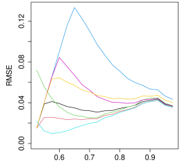
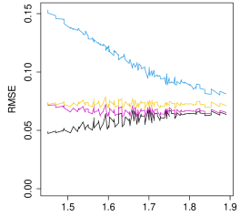
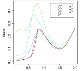
Figure S4: RMSE of the M-estimator in the models M1–M3 as a function of the parameter, based on 1 000 data sets of size $n=5\,000$, $k=800$ (for M1 and M2) and $k=400$ (for M3). Colors represent the seven weight functions from Table S1.

S6.2 Spatial models

Figure S5 shows the distribution of the distances of all the pairs that are used in the analysis in Section 5.2. Figures S6 and S7 present the same results as in Section 5.2 when the estimator (3.9) is used instead of (3.8).

Figure S5: Distribution of the distances $\Delta^{(s)}$ for the 780 pairs used.

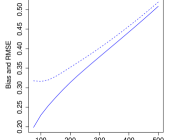
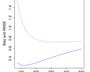
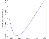
Figure S6: Left and middle columns: Bias (solid line) and RMSE (dotted line) of the estimators of the two spatial parameters $\alpha$ (left) and $\beta$ (middle) as a function of $m$. Right: Mean of the supremum error $\sup_{0\leq\Delta\leq 3}|\theta(\Delta;\widehat{\alpha},\widehat{\beta})-\theta(\Delta;\alpha,\beta)|$ as a function of $m$.

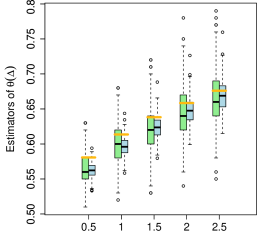
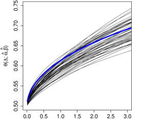
Figure S7: Left panel: Estimators of $\theta(\Delta)$ for 5 different distances. For each distance, bivariate M-estimator $\widehat{\theta}_{n}^{(s)}$ (green) and spatial estimator $\theta(\Delta^{(s)};\widehat{\alpha},\widehat{\beta})$ (blue) based on the $d=40$ locations. Right panel: 50 sampled curves $\theta(\cdot;\widehat{\alpha},\widehat{\beta})$. Blue represents the true curve $\theta(\cdot;\alpha,\beta)$.

References

- Asadi, Davison and Engelke (2015) {barticle}[author] \bauthor\bsnmAsadi, \bfnmP.\binitsP., \bauthor\bsnmDavison, \bfnmA. C.\binitsA. C. and \bauthor\bsnmEngelke, \bfnmS.\binitsS. (\byear2015). \btitleExtremes on river networks. \bjournalAnn. Appl. Stat. \bvolume9 \bpages2023–2050. \endbibitem
- Bingham, Goldie and Teugels (1987) {bbook}[author] \bauthor\bsnmBingham, \bfnmN. H.\binitsN. H., \bauthor\bsnmGoldie, \bfnmC. M.\binitsC. M. and \bauthor\bsnmTeugels, \bfnmJ. L.\binitsJ. L. (\byear1987). \btitleRegular Variation. \bpublisherCambridge University Press. \endbibitem
- Brown and Resnick (1977) {barticle}[author] \bauthor\bsnmBrown, \bfnmBruce M\binitsB. M. and \bauthor\bsnmResnick, \bfnmSidney I\binitsS. I. (\byear1977). \btitleExtreme values of independent stochastic processes. \bjournalJournal of Applied Probability \bvolume14 \bpages732–739. \endbibitem
- Bücher and Dette (2013) {barticle}[author] \bauthor\bsnmBücher, \bfnmAxel\binitsA. and \bauthor\bsnmDette, \bfnmHolger\binitsH. (\byear2013). \btitleMultiplier bootstrap of tail copulas with applications. \bjournalBernoulli \bvolume19 \bpages1655–1687. \endbibitem
- Bücher, Segers and Volgushev (2014) {barticle}[author] \bauthor\bsnmBücher, \bfnmA.\binitsA., \bauthor\bsnmSegers, \bfnmJ.\binitsJ. and \bauthor\bsnmVolgushev, \bfnmS.\binitsS. (\byear2014). \btitleWhen Uniform Weak Convergence Fails: Empirical Processes for Dependence Functions and Residuals via Epi- and Hypographs. \bjournalAnn. Stat. \bvolume42 \bpages1598-1634. \endbibitem
- Bücher, Volgushev and Zou (2019) {barticle}[author] \bauthor\bsnmBücher, \bfnmAxel\binitsA., \bauthor\bsnmVolgushev, \bfnmStanislav\binitsS. and \bauthor\bsnmZou, \bfnmNan\binitsN. (\byear2019). \btitleOn second order conditions in the multivariate block maxima and peak over threshold method. \bjournalJournal of Multivariate Analysis \bvolume173 \bpages604–619. \endbibitem
- Coles, Heffernan and Tawn (1999) {barticle}[author] \bauthor\bsnmColes, \bfnmStuart\binitsS., \bauthor\bsnmHeffernan, \bfnmJanet\binitsJ. and \bauthor\bsnmTawn, \bfnmJonathan\binitsJ. (\byear1999). \btitleDependence measures for extreme value analyses. \bjournalExtremes \bvolume2 \bpages339–365. \endbibitem
- Corless et al. (1996) {barticle}[author] \bauthor\bsnmCorless, \bfnmRobert M\binitsR. M., \bauthor\bsnmGonnet, \bfnmGaston H\binitsG. H., \bauthor\bsnmHare, \bfnmDavid EG\binitsD. E., \bauthor\bsnmJeffrey, \bfnmDavid J\binitsD. J. and \bauthor\bsnmKnuth, \bfnmDonald E\binitsD. E. (\byear1996). \btitleOn the LambertW function. \bjournalAdvances in Computational mathematics \bvolume5 \bpages329–359. \endbibitem
- Csörgő and Horváth (1987) {barticle}[author] \bauthor\bsnmCsörgő, \bfnmMiklós\binitsM. and \bauthor\bsnmHorváth, \bfnmLajos\binitsL. (\byear1987). \btitleApproximation of Intermediate Quantile Processes. \bjournalJournal of multivariate analysis \bvolume21 \bpages250–262. \endbibitem
- Davison and Gholamrezaee (2012) {barticle}[author] \bauthor\bsnmDavison, \bfnmA. C.\binitsA. C. and \bauthor\bsnmGholamrezaee, \bfnmM. M.\binitsM. M. (\byear2012). \btitleGeostatistics of extremes. \bjournalProc. R. Soc. Lond. Ser. A Math. Phys. Eng. Sci. \bvolume468 \bpages581-608. \endbibitem
- Davison, Padoan and Ribatet (2012) {barticle}[author] \bauthor\bsnmDavison, \bfnmAnthony C\binitsA. C., \bauthor\bsnmPadoan, \bfnmSimone A\binitsS. A. and \bauthor\bsnmRibatet, \bfnmMathieu\binitsM. (\byear2012). \btitleStatistical modeling of spatial extremes. \bjournalStatistical science \bvolume27 \bpages161–186. \endbibitem
- de Haan and Ferreira (2006) {bbook}[author] \bauthor\bparticlede \bsnmHaan, \bfnmL.\binitsL. and \bauthor\bsnmFerreira, \bfnmA.\binitsA. (\byear2006). \btitleExtreme Value Theory. \bpublisherSpringer. \endbibitem
- de Haan et al. (2001) {barticle}[author] \bauthor\bparticlede \bsnmHaan, \bfnmLaurens\binitsL., \bauthor\bsnmLin, \bfnmTao\binitsT. \betalet al. (\byear2001). \btitleOn convergence toward an extreme value distribution in C [0, 1]. \bjournalThe Annals of Probability \bvolume29 \bpages467–483. \endbibitem
- de Haan, Neves and Peng (2008) {barticle}[author] \bauthor\bparticlede \bsnmHaan, \bfnmLaurens\binitsL., \bauthor\bsnmNeves, \bfnmCláudia\binitsC. and \bauthor\bsnmPeng, \bfnmLiang\binitsL. (\byear2008). \btitleParametric tail copula estimation and model testing. \bjournalJournal of Multivariate Analysis \bvolume99 \bpages1260–1275. \endbibitem
- Dombry, Engelke and Oesting (2017) {bunpublished}[author] \bauthor\bsnmDombry, \bfnmC.\binitsC., \bauthor\bsnmEngelke, \bfnmS.\binitsS. and \bauthor\bsnmOesting, \bfnmM.\binitsM. (\byear2017). \btitleAsymptotic properties of the maximum likelihood estimator for multivariate extreme value distributions. \bnoteAvailable from https://arxiv.org/abs/1612.05178. \endbibitem
- Draisma et al. (2004) {barticle}[author] \bauthor\bsnmDraisma, \bfnmG.\binitsG., \bauthor\bsnmDrees, \bfnmH.\binitsH., \bauthor\bsnmFerreira, \bfnmA.\binitsA. and \bauthor\bparticlede \bsnmHaan, \bfnmL.\binitsL. (\byear2004). \btitleBivariate Tail Estimation: Dependence in Asymptotic Independence. \bjournalBernoulli \bvolume10 \bpages251-280. \endbibitem
- Drees and Huang (1998) {barticle}[author] \bauthor\bsnmDrees, \bfnmHolger\binitsH. and \bauthor\bsnmHuang, \bfnmXin\binitsX. (\byear1998). \btitleBest attainable rates of convergence for estimators of the stable tail dependence function. \bjournalJournal of Multivariate Analysis \bvolume64 \bpages25–46. \endbibitem
- Einmahl, Krajina and Segers (2008) {barticle}[author] \bauthor\bsnmEinmahl, \bfnmJ. H. J.\binitsJ. H. J., \bauthor\bsnmKrajina, \bfnmA.\binitsA. and \bauthor\bsnmSegers, \bfnmJ.\binitsJ. (\byear2008). \btitleAn method of moments estimator of tail dependence. \bjournalBernoulli \bvolume14 \bpages1003-1026. \endbibitem
- Einmahl, Krajina and Segers (2012) {barticle}[author] \bauthor\bsnmEinmahl, \bfnmJ. H. J.\binitsJ. H. J., \bauthor\bsnmKrajina, \bfnmA.\binitsA. and \bauthor\bsnmSegers, \bfnmJ.\binitsJ. (\byear2012). \btitleAn M-Estimator for Tail Dependence in Arbitrary Dimensions. \bjournalAnn. Stat. \bvolume40 \bpages1764-1793. \endbibitem
- Einmahl, Krajina and Segers (2016) {barticle}[author] \bauthor\bsnmEinmahl, \bfnmJ. H. J.\binitsJ. H. J., \bauthor\bsnmKiriliouk, \bfnmA.\binitsA., \bauthor\bsnmKrajina, \bfnmA.\binitsA. and \bauthor\bsnmSegers, \bfnmJ.\binitsJ. (\byear2016). \btitleAn M-estimator of spatial tail dependence. \bjournalJ. R. Stat. Soc. B \bvolume78 \bpages275-298. \endbibitem
- Einmahl and Segers (2009) {barticle}[author] \bauthor\bsnmEinmahl, \bfnmJohn H. J.\binitsJ. H. J. and \bauthor\bsnmSegers, \bfnmJohan\binitsJ. (\byear2009). \btitleMaximum empirical likelihood estimation of the spectral measure of an extreme-value distribution. \bjournalAnn. Statist. \bvolume37 \bpages2953–2989. \endbibitem
- Engelke and Hitz (2020) {barticle}[author] \bauthor\bsnmEngelke, \bfnmS.\binitsS. and \bauthor\bsnmHitz, \bfnmA. S.\binitsA. S. (\byear2020). \btitleGraphical models for extremes (with discussion). \bjournalJ. R. Stat. Soc. Ser. B Stat. Methodol. \bvolume82 \bpages871–932. \endbibitem
- Engelke and Ivanovs (2021) {barticle}[author] \bauthor\bsnmEngelke, \bfnmS.\binitsS. and \bauthor\bsnmIvanovs, \bfnmJ.\binitsJ. (\byear2021). \btitleSparse Structures for Multivariate Extremes. \bjournalAnnual Review of Statistics and Its Application \bvolume8. \bnoteTo appear. \endbibitem
- Engelke, Opitz and Wadsworth (2019) {barticle}[author] \bauthor\bsnmEngelke, \bfnmSebastian\binitsS., \bauthor\bsnmOpitz, \bfnmThomas\binitsT. and \bauthor\bsnmWadsworth, \bfnmJennifer\binitsJ. (\byear2019). \btitleExtremal dependence of random scale constructions. \bjournalExtremes \bvolume22 \bpages623–666. \endbibitem
- Engelke et al. (2015) {barticle}[author] \bauthor\bsnmEngelke, \bfnmSebastian\binitsS., \bauthor\bsnmMalinowski, \bfnmAlexander\binitsA., \bauthor\bsnmKabluchko, \bfnmZakhar\binitsZ. and \bauthor\bsnmSchlather, \bfnmMartin\binitsM. (\byear2015). \btitleEstimation of Hüsler–Reiss distributions and Brown–Resnick processes. \bjournalJ. R. Stat. Soc. B \bvolume77 \bpages239–265. \endbibitem
- Guillotte, Perron and Segers (2011) {barticle}[author] \bauthor\bsnmGuillotte, \bfnmSimon\binitsS., \bauthor\bsnmPerron, \bfnmFrançois\binitsF. and \bauthor\bsnmSegers, \bfnmJohan\binitsJ. (\byear2011). \btitleNon-parametric Bayesian inference on bivariate extremes. \bjournalJ. R. Stat. Soc. B \bvolume73 \bpages377–406. \endbibitem
- Gumbel (1960) {barticle}[author] \bauthor\bsnmGumbel, \bfnmEmil Julius\binitsE. J. (\byear1960). \btitleDistributions des valeurs extremes en plusiers dimensions. \bjournalPubl. Inst. Statist. Univ. Paris \bvolume9 \bpages171–173. \endbibitem
- Heffernan and Resnick (2007) {barticle}[author] \bauthor\bsnmHeffernan, \bfnmJanet E.\binitsJ. E. and \bauthor\bsnmResnick, \bfnmSidney I.\binitsS. I. (\byear2007). \btitleLimit laws for random vectors with an extreme component. \bjournalAnn. Appl. Probab. \bvolume17 \bpages537–571. \endbibitem
- Heffernan and Tawn (2004) {barticle}[author] \bauthor\bsnmHeffernan, \bfnmJ. E.\binitsJ. E. and \bauthor\bsnmTawn, \bfnmJ. A.\binitsJ. A. (\byear2004). \btitleA conditional approach for multivariate extreme values (with discussion). \bjournalJ. R. Stat. Soc. Ser. B Stat. Methodol. \bvolume66 \bpages497–546. \endbibitem
- Huang (1992) {bphdthesis}[author] \bauthor\bsnmHuang, \bfnmX.\binitsX. (\byear1992). \btitleStatistics of Bivariate Extreme Value Theory, \btypePhD thesis, \bpublisherErasmus University Rotterdam. \endbibitem
- Huser, Opitz and Thibaud (2017) {barticle}[author] \bauthor\bsnmHuser, \bfnmR.\binitsR., \bauthor\bsnmOpitz, \bfnmT.\binitsT. and \bauthor\bsnmThibaud, \bfnmE.\binitsE. (\byear2017). \btitleBridging asymptotic independence and dependence in spatial extremes using Gaussian scale mixtures. \bjournalSpatial Statistics \bvolume21 \bpages166 - 186. \endbibitem
- Huser and Wadsworth (2019) {barticle}[author] \bauthor\bsnmHuser, \bfnmRaphaël\binitsR. and \bauthor\bsnmWadsworth, \bfnmJennifer L\binitsJ. L. (\byear2019). \btitleModeling spatial processes with unknown extremal dependence class. \bjournalJournal of the American Statistical Association \bvolume114 \bpages434–444. \endbibitem
- Hüsler and Reiss (1989) {barticle}[author] \bauthor\bsnmHüsler, \bfnmJürg\binitsJ. and \bauthor\bsnmReiss, \bfnmRolf-Dieter\binitsR.-D. (\byear1989). \btitleMaxima of normal random vectors: between independence and complete dependence. \bjournalStatistics & Probability Letters \bvolume7 \bpages283–286. \endbibitem
- Kabluchko et al. (2009) {barticle}[author] \bauthor\bsnmKabluchko, \bfnmZakhar\binitsZ., \bauthor\bsnmSchlather, \bfnmMartin\binitsM., \bauthor\bsnmDe Haan, \bfnmLaurens\binitsL. \betalet al. (\byear2009). \btitleStationary max-stable fields associated to negative definite functions. \bjournalThe Annals of Probability \bvolume37 \bpages2042–2065. \endbibitem
- Keef, Tawn and Svensson (2009) {barticle}[author] \bauthor\bsnmKeef, \bfnmC.\binitsC., \bauthor\bsnmTawn, \bfnmJ.\binitsJ. and \bauthor\bsnmSvensson, \bfnmC.\binitsC. (\byear2009). \btitleSpatial risk assessment for extreme river flows. \bjournalJ. R. Stat. Soc. Ser. C. Appl. Stat. \bvolume58 \bpages601–618. \endbibitem
- Kosorok (2008) {bbook}[author] \bauthor\bsnmKosorok, \bfnmM. R.\binitsM. R. (\byear2008). \btitleIntroduction to Empirical Processes and Semiparametric Inference. \bpublisherSpringer. \endbibitem
- Le et al. (2018) {barticle}[author] \bauthor\bsnmLe, \bfnmPhuong Dong\binitsP. D., \bauthor\bsnmDavison, \bfnmAnthony C\binitsA. C., \bauthor\bsnmEngelke, \bfnmSebastian\binitsS., \bauthor\bsnmLeonard, \bfnmMichael\binitsM. and \bauthor\bsnmWestra, \bfnmSeth\binitsS. (\byear2018). \btitleDependence properties of spatial rainfall extremes and areal reduction factors. \bjournalJ. Hydrol. \bvolume565 \bpages711–719. \endbibitem
- Ledford and Tawn (1996) {barticle}[author] \bauthor\bsnmLedford, \bfnmAnthony W\binitsA. W. and \bauthor\bsnmTawn, \bfnmJonathan A\binitsJ. A. (\byear1996). \btitleStatistics for near independence in multivariate extreme values. \bjournalBiometrika \bvolume83 \bpages169–187. \endbibitem
- Ledford and Tawn (1997) {barticle}[author] \bauthor\bsnmLedford, \bfnmA. W.\binitsA. W. and \bauthor\bsnmTawn, \bfnmJ. A.\binitsJ. A. (\byear1997). \btitleModelling Dependence within Joint Tail Regions. \bjournalJ. R. Stat. Soc. B \bvolume59 \bpages475–499. \endbibitem
- Padoan, Ribatet and Sisson (2010) {barticle}[author] \bauthor\bsnmPadoan, \bfnmS. A.\binitsS. A., \bauthor\bsnmRibatet, \bfnmM.\binitsM. and \bauthor\bsnmSisson, \bfnmS. A.\binitsS. A. (\byear2010). \btitleLikelihood-based inference for max-stable processes. \bjournalJ. Amer. Statist. Assoc. \bvolume105 \bpages263–277. \endbibitem
- Peng (1999) {barticle}[author] \bauthor\bsnmPeng, \bfnmLiang\binitsL. (\byear1999). \btitleEstimation of the coefficient of tail dependence in bivariate extremes. \bjournalStat. & Probab. Lett. \bvolume43 \bpages399–409. \endbibitem
- Peng and Qi (2008) {barticle}[author] \bauthor\bsnmPeng, \bfnmLiang\binitsL. and \bauthor\bsnmQi, \bfnmYongcheng\binitsY. (\byear2008). \btitleBootstrap approximation of tail dependence function. \bjournalJournal of Multivariate Analysis \bvolume99 \bpages1807–1824. \endbibitem
- Poon, Rockinger and Tawn (2004) {barticle}[author] \bauthor\bsnmPoon, \bfnmS. H.\binitsS. H., \bauthor\bsnmRockinger, \bfnmM.\binitsM. and \bauthor\bsnmTawn, \bfnmJ.\binitsJ. (\byear2004). \btitleExtreme Value Dependence in Financial Markets: Diagnostics, Models, and Financial Implications. \bjournalRev. Financ. Stud. \bvolume17 \bpages581-610. \endbibitem
- Ramos and Ledford (2009) {barticle}[author] \bauthor\bsnmRamos, \bfnmA.\binitsA. and \bauthor\bsnmLedford, \bfnmA.\binitsA. (\byear2009). \btitleA new class of models for bivariate joint tails. \bjournalJ. R. Stat. Soc. B \bvolume71 \bpages219-241. \endbibitem
- Resnick (1987) {bbook}[author] \bauthor\bsnmResnick, \bfnmSidney I\binitsS. I. (\byear1987). \btitleExtreme values, regular variation and point processes. \bpublisherSpringer. \endbibitem
- Resnick (2002) {barticle}[author] \bauthor\bsnmResnick, \bfnmSidney\binitsS. (\byear2002). \btitleHidden Regular Variation, Second Order Regular Variation and Asymptotic Independence. \bjournalExtremes \bvolume5 \bpages303–336. \endbibitem
- Rockafellar (1970) {bbook}[author] \bauthor\bsnmRockafellar, \bfnmR Tyrrell\binitsR. T. (\byear1970). \btitleConvex Analysis \bvolume28. \bpublisherPrinceton university press. \endbibitem
- Schlather (2002) {barticle}[author] \bauthor\bsnmSchlather, \bfnmM.\binitsM. (\byear2002). \btitleModels for Stationary Max-Stable Random Fields. \bjournalExtremes \bvolume5 \bpages33-44. \endbibitem
- Smith (1990) {bmisc}[author] \bauthor\bsnmSmith, \bfnmR. L.\binitsR. L. (\byear1990). \btitleMax-Stable Processes and Spatial Extremes. \bhowpublishedUnpublished manuscript. \endbibitem
- Tawn (1988) {barticle}[author] \bauthor\bsnmTawn, \bfnmJ. A.\binitsJ. A. (\byear1988). \btitleBivariate Extreme Value Theory: Models and Estimation. \bjournalBiometrika \bvolume75 \bpages397-415. \endbibitem
- Teschl (1998) {bbook}[author] \bauthor\bsnmTeschl, \bfnmGerald\binitsG. (\byear1998). \btitleTopics in Real and Functional Analysis. \bpublisherUnpublished, available online at https://www.mat.univie.ac.at/gerald/ftp/book-fa. \endbibitem
- van der Vaart (2000) {bbook}[author] \bauthor\bparticlevan der \bsnmVaart, \bfnmAad W\binitsA. W. (\byear2000). \btitleAsymptotic statistics. \bpublisherCambridge university press. \endbibitem
- van der Vaart and Wellner (1996) {bbook}[author] \bauthor\bparticlevan der \bsnmVaart, \bfnmAad W\binitsA. W. and \bauthor\bsnmWellner, \bfnmJon A\binitsJ. A. (\byear1996). \btitleWeak Convergence and Empirical Processes With Applications to Statistics. \bpublisherSpringer. \endbibitem
- Vervaat (1972) {barticle}[author] \bauthor\bsnmVervaat, \bfnmW.\binitsW. (\byear1972). \btitleFunctional Central Limit Theorems for Processes with Positive Drift and Their Inverses. \bjournalZ. Wahrscheinlichkeitstheorie Verw. Geb. \bvolume23 \bpages245-253. \endbibitem
- Wadsworth and Tawn (2012) {barticle}[author] \bauthor\bsnmWadsworth, \bfnmJ. L.\binitsJ. L. and \bauthor\bsnmTawn, \bfnmJ. A.\binitsJ. A. (\byear2012). \btitleDependence modelling for spatial extremes. \bjournalBiometrika \bvolume99 \bpages253–272. \endbibitem
- Wadsworth et al. (2017) {barticle}[author] \bauthor\bsnmWadsworth, \bfnmJL\binitsJ., \bauthor\bsnmTawn, \bfnmJonathan Angus\binitsJ. A., \bauthor\bsnmDavison, \bfnmAC\binitsA. and \bauthor\bsnmElton, \bfnmDaniel Mark\binitsD. M. (\byear2017). \btitleModelling across extremal dependence classes. \bjournalJournal of the Royal Statistical Society: Series B (Statistical Methodology) \bvolume79 \bpages149–175. \endbibitem
- Weller and Cooley (2014) {barticle}[author] \bauthor\bsnmWeller, \bfnmG. B.\binitsG. B. and \bauthor\bsnmCooley, \bfnmD.\binitsD. (\byear2014). \btitleA sum characterization of hidden regular variation with likelihood inference via expectation-maximization. \bjournalBiometrika \bvolume101 \bpages17–36. \endbibitem
- Westra and Sisson (2011) {barticle}[author] \bauthor\bsnmWestra, \bfnmS.\binitsS. and \bauthor\bsnmSisson, \bfnmS. A.\binitsS. A. (\byear2011). \btitleDetection of non-stationarity in precipitation extremes using a max-stable process model. \bjournalJournal of Hydrology \bvolume406 \bpages119 – 128. \endbibitem
- Zhou (2010) {barticle}[author] \bauthor\bsnmZhou, \bfnmC.\binitsC. (\byear2010). \btitleDependence structure of risk factors and diversification effects. \bjournalInsur. Math. Econ. \bvolume46 \bpages531–540. \endbibitem
- Zscheischler and Seneviratne (2017) {barticle}[author] \bauthor\bsnmZscheischler, \bfnmJakob\binitsJ. and \bauthor\bsnmSeneviratne, \bfnmSonia I.\binitsS. I. (\byear2017). \btitleDependence of drivers affects risks associated with compound events. \bjournalScience Advances \bvolume3. \endbibitem