Estimating undocumented Covid-19 infections in Cuba by means of a hybrid mechanistic-statistical approach

Abstract

We adapt the hybrid mechanistic-statistical approach of Ref. roques2020 to estimate the total number of undocumented Covid-19 infections in Cuba. This scheme is based on the maximum likelihood estimation of a SIR-like model parameters for the infected population, assuming that the detection process matches a Bernoulli trial. Our estimations show that (a) $60\%$ of the infections were undocumented, (b) the real epidemics behind the data peaked ten days before the reports suggested, and (c) the reproduction number swiftly vanishes after 80 epidemic days.

INTRODUCTION

Covid-19 crisis has put forward the need for simple and yet realistic epidemic modeling. The goal is to provide the authorities and the public with accurate predictions to devise and schedule containment and organization policies before an outbreak peaks. To this effect, the daily number of new infections and a minimal description of the epidemic peak (the so-called acme), in terms of the date and number of active infections, are among the crucial data. Another quantity of concern, especially relevant to grasp the full extent of an epidemics –as well as to assess detection strategies– is the total number of active infections per day. Due to the fact that there is always a fraction of infections that is not detected, a fortiori when the pathogen may be carried asymptomatically (e.g., the case of SARS-CoV-2), the full infected population can only be inferred.

In particular, estimations of total Covid-19 infections (including undocumented trasmission events) are already available in the literature for France roques2020 and China li2020 , but are still unknown to many other countries. To the best of our knowledge, there are no current estimates of total Covid-19 infections in Cuba. Therefore, this paper aims at contributing such an important piece of information to the modeling of the pandemics in Cuba.

Historically, epidemic modeling is dominated by mechanistic approaches, like SIS, SIR and SEIR (where letters in the acronyms stands for susceptible, exposed, infected and recovered compartments of the population) mandal2011 . The advantage of a mechanistic model is that it sets up the epidemic evolution from reasonable time-dependent rules for trasmission and recovery (the mechanics behind the epidemics, so to say). Often, such a mechanical description applies to the full infected population. A straightforward (brute-force) fitting of mechanistic models (e.g., the typical SIR) to just the reported data may not be the correct strategy to follow, since, on one hand, detection draws from statistical sampling of the full infected population, and, on the other, there are detected cases with unknown source of contagion (i.e., unable to stem from the interaction between the infected and susceptible compartments, as modeled).

There have been some efforts directed at reconciling a mechanistic approach with the intrinsic statistical nature of the reported data breto2009 ; li2018 . In particular, we are inspired by the hybrid mechanistic-statistical (HMS) approach laid down in Ref. roques2020 , which was succesful at modeling Covid-19 in France.

The HMS scheme by Roques et al. applies Bayesian inference to estimate SIR parameters (and, hence, the total infected population), assuming that the detection process accomodates to a Bernoulli trial roques2020 . Since we are interested in limited outbreaks, where government measures are effective at containing the disease, we can choose a simplification of the general SIR model that considers the infected cases negligible with repect to the full population. Moreover, in the same spirit of Cabo-Cabo (fully mechanistic) modeling of Covid-19 in Cuba cabo2020 , we simulate the effect of the state interventions by means of a heuristic time-dependence of the infection rate, dropping down the day the most strigent measures against spreading were implemented. We also correct the statistical part of the HMS as formulated in Ref. roques2020 , by considering that only the still undocumented portion of the infected cases are sampled for test.

The outline of the paper is the following. Sec. I summarizes the mechanistic and the statistical side of the hybrid approach, emphasizing our ammendments to the formulation in Ref. roques2020 . Sec. II describe the validation scheme and computations. Sec. III tackle two epidemic scenarios: a synthetic outbreak and the case of Covid-19 in Cuba. In Sec. IV, we provide some concluding remarks. In the Appendix, we comment on how the synthetic epidemics (used for validation purposes) was generated.

I Methods

Mechanics: simplified SIR model with a heuristic time-dependent infection rate

We start from the most customary Susceptible + Infected + Recovered (SIR) model, introduced by Kermack and McKendrick kermack-mckendrick1927 , i.e.,

$$\frac{dS(t)}{dt} = -\alpha\frac{I(t)S(t)}{N}~{},$$ (1)

$$\frac{dI(t)}{dt} = \alpha\frac{I(t)S(t)}{N}-\beta I(t)~{},$$ (2)

$$\frac{dR(t)}{dt} = \beta I(t)~{}.$$ (3)

$S(t)$, $I(t)$ and $R(t)$ are the susceptible, infected and recovered time-dependent populations, which sum up to the size of the full population $N$ (i.e., $S(t)+I(t)+R(t)=N$), whereas $\alpha$ and $\beta$ are the infection and recovery rates. Time $t$ is given in days, hereafter. The cumulative number of infections within a timespan reads

$$T(t)=I(t)+R(t)~{}.$$ (4)

At difference with Ref. roques2020 , we take a reasonable simplification of the usual SIR model valid for a more or less contained outburst or an early stage of the epidemics cabo2020 . In such a case, $T(t)\ll N$ and $S(t)\approx N$. Therefore, the infected population reads

$$I(t)=I_{0}\exp{\left\{(R_{0}-1)~{}\beta~{}(t-t_{0})\right\}}~{},$$ (5)

where $R_{0}=\alpha/\beta$ is the basic reproduction number, and $I(t_{0})=I_{0}$ is the initial number of infections. From Eq. (5), we note that an exponential increase or decrease of infectious events takes place depending on whether $R_{0}$ is greater or lesser than the unity.

Now, let the infection rate be time-dependent. In such a case, we get

$$I(t)=I_{0}\exp{\left\{\int_{t_{0}}^{t}\alpha(t^{\prime})~{}dt^{\prime}-\beta~{}(t-t_{0})\right\}}~{},$$ (6)

instead of Eq. (5). We assume a heuristic shape for such a time-dependence, for example, a step function taking a constant value at the beginning ($\alpha_{0}>\beta$, to allow for an outbreak) and dropping down to a lower value ($\alpha_{\infty}<\alpha_{0}$) at some point in time, $t_{1}$. For a country suffering an epidemics, we set such an inflection point to the day borders were closed or a stringency index jumps abruptly stringency . In particular, we choose a Fermi-Dirac distribution as a smooth version of the step function, i.e.,

$$\alpha(t)=\frac{\Delta\alpha}{1+e^{(t-t_{1})/\tau}}+\alpha_{\infty}~{},$$ (7)

where $\alpha_{0}\equiv\alpha(t_{0})=\Delta\alpha/(1+e^{(t_{0}-t_{1})/\tau})+\alpha_{\infty}$, $\alpha_{1}\equiv\alpha(t_{1})=\Delta\alpha+\alpha_{\infty}$, $\alpha_{\infty}\equiv\lim_{t\to\infty}\alpha(t)$ and $\tau$ is a smooth parameter modulating how fast the infection rate drops down from $\alpha_{0}$ to $\alpha_{\infty}$. From Eqs. (6) and (7), we get

$$I(t)= I_{0}\exp{\{(\alpha_{1}-\beta)(t-t_{0})}\}\times$$ (8)

$$\left(\frac{(1+\exp\{(t_{0}-t_{1})/\tau\})}{(1+\exp\{(t-t_{1})/\tau\})}\right)^{\Delta\alpha\tau}~{},$$

Models relying on heuristic time-dependent infection rates that swiftly vanish after lockdown and stringent measures from the government have been recently explored in Ref. cabo2020 .

Statistics: testing as a binomial process and maximum likelihood inference of SIR parameters

Let us assume that the daily detection of new infected cases $\delta_{t}$ is a Bernoulli process, as in Ref. roques2020 . Hence, the random variable $\delta_{t}$ distributes binomially,

$$\delta_{t}\sim\mathrm{Bin}(n_{t},p_{t})~{},$$ (9)

where $n_{t}$ is the number of trials (i.e., the daily size of the test sample) and $p_{t}$, the probability of success in each independent trial (for us, the probability of finding infected cases in the population). Subindex $t$ is kept throughout for time series data.

In such a Bernoulli process, test outcomes are independent from each other. For that to happen, the sample for test would have to be selected at random from the full population. However, more effective and realistic testing strategies often departs from random sampling by focusing on trasmission chains and/or risk groups. To simulate higher prevalence in test samples as compared to random ones, we assume that susceptible population will always be under-sampled, i.e., we bias the probability of finding positive results. In Ref. roques2020 ,

$$p_{t}=\frac{I(t)}{I(t)+\kappa S(t)}$$ (10)

where $\kappa\in(0,1)$.

At odds with Eq. (10), we account for the fact that there is a fraction of the infected population that once tested is quarantined and their retests are not contemplated in $\delta_{t}$. To that aim, $p_{t}$ does not builds up from the total but from the currently infected cases that are yet undocumented, i.e., the difference between the full infected population and the active (positive to the test) cases just the day before the current tests, $\mathrm{A}_{t-1}$. Again, we take $S(t)\approx N$. Therefore, Eq. (10) is replaced by

$$p_{t}=\frac{I(t)-\mathrm{A}_{t-1}}{I(t)-\mathrm{A}_{t-1}+\kappa N}~{}.$$ (11)

The likelihood of detecting daily reported cases $\delta_{t}$ given an infected population evolving a là SIR (see Eq. (8)) and assuming testing outcomes can be accommodated into a Bernoulli process is roques2020

$$\mathcal{L}(I_{0},\Delta\alpha,\alpha_{\infty},\tau,\kappa)=\Pi_{t=t_{0}}^{t_{f}}\left(\begin{array}[]{c}n_{t}\\ \delta_{t}\end{array}\right)p_{t}^{\delta_{t}}(1-p_{t})^{n_{t}-\delta_{t}}~{}.$$ (12)

Here, all the parameters are encoded into $p_{t}$, in the case of SIR parameters ($I_{0}$, $\Delta\alpha$, $\alpha_{\infty}$ and $\tau$), through the infected population $I(t)$ (see Eqs.  (8) and (11)). Supposing parameters distribute uniformly within the searched domain, the maximization of the likelihood $\mathcal{L}$ lead us to the SIR infected evolution that best reproduce the reported data on daily new cases (in the sense of having the largest probability of being the specific dynamics behind the data). The biasing parameter $\kappa$ is also inferred by maximizing the likelihood.

II Validation and computational details

As anticipated, we want to use our model to estimate the number of total infected population over time from the reported data. Since the motivation for developing such a model is precisely the fact that there are undocumented infections, we do not have an immediate way of validating our results. Roques et al. roques2020 carried out an indirect validation, by comparing actual data on infected cases with the expected number of the corresponding, binomially distributed, random variable (actually, the cumulative over time of such quantities was employed). Here, we propose as well a direct validation scheme by means of a network epidemic model (NEM). In a nutshell, such a NEM builds up from an unconstrained spread and a detection/quarantine process based on symptomatic cases and traceable trasmission chains they point at (see the Appendix for details). Although, the NEM deserves attention in its own right, its full presentation and analysis is outside the scope of this article and will be published elsewhere. In this paper, it only provides a synthetic epidemic scenario where the total infected population is known by construction, therefore, setting a benchmark for our hybrid model estimation (introduced in earlier sections).

The HMS model is implemented in a Wolfram Mathematica 11.3 notebook (available upon request to the authors). The maximum likelihood estimation (MLE) is carried out through a Nelder-Mead global optimization method with a maximum of $10^{3}$ iterations. We impose the natural constraints on the parameters (i.e., $\Delta\alpha\geq 0$, $\alpha_{\infty}\geq 0$, $\tau\geq 0$, $I_{0}>0$ and $\kappa\in(0,1)$) together with $\alpha_{0}\equiv\Delta\alpha/\left(1+\exp{(t_{0}-t_{1}/\tau)}\right)+\alpha_{\infty}>1$, to allow for an initial outbreak. As a matter of fact, we do not maximize the likelihood $\mathcal{L}$ itself (see Eq. (12)) but $\ln{(\mathcal{L})}$, which is a smoother function of the parameters. We set $N\approx 11\times 10^{6}$, approximately the Cuban population. To model the outbreak of Covid-19 in Cuba, we set $1/\beta=20~{}\mathrm{days}$ zhou2020 and $t_{1}$ to the 13th epidemic day, i.e., the day borders and schools were closed and stringency index took the largest leap ($25$ out of a maximum of $100$ units) data1 . Covid-19 data for Cuba is taken from data1 ; data2 . For the MLE in Cuba, we use only the first 80 days, which include an almost complete epidemic peak. Our SIR cannot capture the two-peak profile actually seen in the number of active cases reported for Covid-19 in Cuba (see Fig. 2), so far as 110 epidemic days. The number of daily PCR tests for Covid-19 as reported by the Cuban Ministry of Health is a tricky figure in many senses: for example, it is not clear whether it includes or not (a) retests of already detected cases and (b) tests for which the result might be pending test . Not having a more intuitive way of estimating the daily number of tests, we choose a constant value for the number of daily tests and set it to the geometric mean of the reported daily Covid-19 tests data in Cuba in a period of 110 epidemic days (i.e., $n_{t}\approx 1500$). For the synthetic epidemics (our validation case), we change abruptly the reproduction number at the 43rd day (so, we can set $t_{1}=43~{}\mathrm{days}$) and choose a recovery time of $1/\beta=7~{}\mathrm{days}$. The number of tests is the same as for the Covid-19-in-Cuba scenario.

III Results

A synthetic epidemic scenario

Figure 1 shows our results on HMS estimations of the extent of a simulated epidemic outburst, where the total number of active cases is known by construction. Remarkably, such estimations are in a good agreement with the actual benchmark data during the early stages of the outbreak. The quality of our estimation after the epidemics has peaked is poor, but note that they are at least able to spot accurately the date of the acme. Together with our HMS estimations, we plot a non-linear regression model as applied to the total number of active cases. Both the HMS and the regression models have the same functional dependence on time, given by Eq. (8), and target the same quantity (i.e., the total number of active cases). The practical difference between the two is in the input data: whereas HMS builds up from data on the active and newly detected cases per day, the other directly fits the usually unknown total number of active cases. We do not expect that HMS approach achieve the same degree of success of a fit, since the underlying method does not try to make $I(t)$ conform to the total number of active cases, e.g., by minimizing their relative differences. At odds with a regression, the HMS maximizes the chances of obtaining newly detected cases per day out of a statistical sampling of a proxy for yet undocumented infections (i.e., $I(t)-\mathrm{A}_{t-1}$). The advantage of HMS is that it is useful in all realistic situations in which the total number of active cases is simply not available due to undocumented infections.

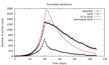
Figure 1: (color online) Total number of active cases for a simulated epidemics (full circles) and our HMS estimation of the same quantity (solid red line). We also show a fit of Eq. (8) to the total number of active cases (dashed blue line). As a reference, we plot the reported number of active cases (empty circles), which is the input of our HMS estimation.

Covid-19 in Cuba

As seen in the last section, HMS works well at the epidemic outburst, providing reasonable estimates of the total number of cases and the date of the full epidemic curve (which need not to coincide with the peak of the reported data). Thus validated, we proceed to apply HMS to the recent Covid-19 epidemics in Cuba. In Fig. 2, we show a comparison between active cases as obtained from official reports and our estimates (which includes undocumented infections). The full epidemic curve peaks ten days before the reported one. Day by day, reported infections ranges from $4$ to $49\%$ of the total, with a mean of $28\%$, achieved at the full acme. Remarkably, the cumulative number of reported infections within the timespan of 80 days was about $40\%$ of the total (see Eq. (4)), and $T/N=4.6\times 10^{-4}$. These are fingerprints of good management of Covid-19 medical crisis in Cuba (cf. Ref. li2020 ’s estimate of $14\%$ of documented infections in China before the travel restrictions on 23 January 2020). Moreover, notice that the fraction of documented infections increase over time, from an initial value of $11\%$ to the aforementioned $40\%$, indicating a refinement in Cuban detection process during the epidemics.

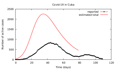
Figure 2: (color online) Number of active cases of Covid-19 in Cuba (black dots), together with our HMS estimation of the total number of active cases (solid red line), including undocumented infections.

In the case of Covid-19 in Cuba, we can only appeal to an indirect validation of our HMS estimates. Fig. 2 shows the cumulative number of reported infections, $\sum_{t\prime=t_{0}}^{t}\delta_{t\prime}$, along with its expected value within our Bernoulli process, $\sum_{t\prime=t_{0}}^{t}n_{t\prime}p_{t\prime}$. Good agreement is generally obtained (mean and standard deviation of around 9 and 28 cases, respectively), and nearly zero relative difference at the end of the interval (80 days).

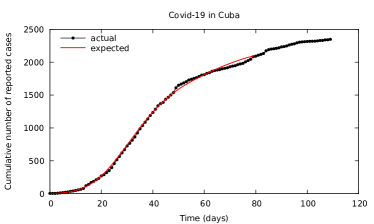
Figure 3: (color online) Cumulative number of reported cases of Covid-19 in Cuba (black dots) along with the expected number of the same quantity by means of HMS (solid red line).

Table 1: Summary of the parameters obtained for each modeling presented in this paper. $R_{0}^{(0)}=\alpha_{0}/\beta$ is the reproduction number the first epidemic day, $R_{0}^{(\infty)}=\alpha_{\infty}/\beta$ is its asymptotic value and $\widetilde{\kappa}=\kappa\times 10^{3}$.

Epidemics	$I_{0}$	$R_{0}^{(0)}$	$R_{0}^{(\infty)}$	$\tau$ (days)	$\widetilde{\kappa}$
NEM simulated	7.81	1.92	0.69	0.86	3.9
Covid-19 in Cuba	32.47	6.39	0.02	11.17	4.0

Table 1 summarizes the parameters we get for both, the simulated epidemics and Covid-19 in Cuba. In the latter case, we emphasize the jump in reproduction number the day borders and schools were closed, from 6.39 at the beginning to nearly zero the 80th epidemic day (cf. cabo2020 ).

IV Concluding remarks

We adapted the hybrid mechanistic-statistical method developed by Roques et al. roques2020 , already succesful at modeling Covid-19 in France, to be able to make reasonable estimations of total Covid-19 infections in Cuba. Our theoretical contribution is two-fold. On one hand, we chose a heuristic modification of the classical SIR model that assumes limited outbreaks together with an infection rate changing abruptly when stringent measures take place (see also Ref. cabo2020 ). On the other hand, we corrected the probability entering the binomial distribution of newly detected cases, in order to account for the fact that the daily reports do not include retest outcomes of already detected cases. Both ammendments turn out to be essential when modeling Covid-19 in Cuba.

Furthermore, we provided a testing ground for the hybrid mechanistic-statistical estimations: the case of a network epidemic simulation where the total number of active cases is known by construction. The hybrid model is validated against such a benchmark, at least in the early stages of the outburst before the epidemics peaks.

Applying the hybrid model to Covid-19 in Cuba allows us to estimate the total number of active cases, including undocumented infections. The resulting number of undocumented Covid-19 infections in Cuba reaches $60\%$, which is considerably less than the estimate for China ($86\%$) before the travel restrictions were implemented li2020 , therefore, indicating a good management of the medical crisis in Cuba.

References

- [1] L. Roques, E. K. Klein, J. Papaïx, A. Sar, and S. Soubeyrand. Using early data to estimate the actual infection fatality ratio from COVID-19 in France. Biology, 9:97, 2020.
- [2] R. Li, S. Pei, B. Chen, Y. Song, T. Zhang, W. Yang, and J. Shaman. Substantial undocumented infection facilitates the rapid dissemination of novel coronavirus (SARS-CoV2). Science, 368:489–493, 2020.
- [3] S. Mandal, R. R. Sarkar, and S. Sinha. Mathematical models of malaria - a review. Malaria Journal, 10:202, 2011.
- [4] C. Bretó, D. He, E. L. Ionides, and A. King. Time series analysis via mechanistic models. The Annals of Applied Statistics, 3(1):319–348, 2009.
- [5] M. Li, J. Dushoff, and B.M. Bolker. Fitting mechanistic epidemic models to data: A comparison of simple Markov chain Monte Carlo approaches. Statistical Methods in Medical Research, 27(7):1956–1967, 2018.
- [6] N. Cabo-Bizet and A. Cabo Montes de Oca. Modelos SIR modificados para la evolución del COVID19. arXiv:2004.11352v1, 2020.
- [7] W.O. Kermack and A.G. McKendrick. A Contribution to the Mathematical Theory of Epidemics. Proceedings of the Royal Society A, 1927.
- [8] www.bsg.ox.ac.uk/covidtracker.
- [9] F. Zhou, T. Yu, R. Du, G. Fan, Y. Liu, Z. Liu, J. Xiang, Y. Wang, B. Song, and X. Gu et al. Clinical course and risk factors for mortality of adult inpatients with COVID-19 in Wuhan, China: a retrospective cohort study. The Lancet, 395:10229, 2020.
- [10] https://covid19cubadata.github.io.
- [11] https://github.com/pomber/covid19.
- [12] https://ourworldindata.org/coronavirus-testing#cuba.