Multi-Stage Optimized Machine Learning Framework for Network Intrusion Detection

Abstract

Cyber-security garnered significant attention due to the increased dependency of individuals and organizations on the Internet and their concern about the security and privacy of their online activities. Several previous machine learning (ML)-based network intrusion detection systems (NIDSs) have been developed to protect against malicious online behavior. This paper proposes a novel multi-stage optimized ML-based NIDS framework that reduces computational complexity while maintaining its detection performance. This work studies the impact of oversampling techniques on the models’ training sample size and determines the minimal suitable training sample size. Furthermore, it compares between two feature selection techniques, information gain and correlation-based, and explores their effect on detection performance and time complexity. Moreover, different ML hyper-parameter optimization techniques are investigated to enhance the NIDS’s performance. The performance of the proposed framework is evaluated using two recent intrusion detection datasets, the CICIDS 2017 and the UNSW-NB 2015 datasets. Experimental results show that the proposed model significantly reduces the required training sample size (up to 74%) and feature set size (up to 50%). Moreover, the model performance is enhanced with hyper-parameter optimization with detection accuracies over 99% for both datasets, outperforming recent literature works by 1-2% higher accuracy and 1-2% lower false alarm rate.

I Introduction

The Internet has become an essential aspect of daily life with individuals and organizations depending on it to facilitate communication, conduct business, and store information [1, 2]. This dependence is coupled with these individuals and organizations’ concern about the security and privacy of their online activities [3]. Accordingly, the area of cyber-security has garnered significant attention from both the industry and academia. To that end, more resources are being deployed and allocated to protect modern Internet-based networks from potential attacks or anomalous activities. Several protection mechanisms have been proposed such as firewalls, user authentication, and the deployment of antivirus and malware programs as a first line of defense [4]. However, these mechanisms have not been able to completely protect the organizations’ networks, particularly with contemporary attacks [5].
Typically, network intrusion detection systems (NIDSs) can be divided into two main categories: signature-based detection systems (misused detection) and anomaly-based detection systems [6]. Signature-based detection systems base their detection on the observation of pre-defined attack patterns. Thus, they have proven to be effective for attacks with well-known signatures and patterns. However, these systems are vulnerable against new attacks due to their inability to detect new attacks by learning from previous observations [7]. In contrast, anomaly-based detection systems base their detection on the observation of any behavior or pattern that deviates from what is considered to be normal. Therefore, these systems can detect unknown attacks or intrusions based on the built models that characterize normal behavior [8].
Despite the continuous improvements in NIDS performance, there is still room for further improvement. This is particularly evident given the high volume of generated network traffic data, continuously evolving environments, vast amounts of features collected that form the training datasets (high dimensional datasets), and the need for real-time intrusion detection [9]. For example, having redundant or irrelevant features can have a negative impact on the detection capabilities of NIDSs as it slows down the model training process. Therefore, it is important to choose the most suitable subset of features and optimize the parameters of the machine learning (ML)-based detection models to enhance their performance [10].
This paper extends our previous work in [11] by proposing a novel multi-stage optimized ML-based NIDS framework that reduces the computational complexity while maintaining its detection performance. To that end, this work first studies the impact of oversampling techniques on the models’ training sample size and determines the minimum suitable training size for effective intrusion detection. Furthermore, it compares between two different feature selection techniques, namely information gain and correlation-based feature selection, and explores their effect on the models’ detection performance and time complexity. Moreover, different ML hyper-parameter optimization techniques are investigated to enhance the NIDS’s performance and ensure its effectiveness and robustness.
To evaluate the performance of the proposed optimized ML-based NIDS framework, two recent state-of-the-art intrusion detection datasets are used, namely the CICIDS 2017 dataset [12] (which is the updated version of the ISCX 2012 dataset [13] used in our previous work [11]) and the UNSW-NB 2015 dataset [14]. The performance evaluation is conducted using various evaluation metrics such as accuracy (acc), precision, recall, and false alarm rate (FAR).
The remainder of this paper is organized as follows: Section II briefly summarizes some of the previous literature works that focused on this research problem and presents its limitations. Section III summarizes the contributions of this work. Section IV discusses the theoretical mathematical background of the different deployed techniques. Section V presents the proposed multi-stage optimized ML-based NIDS framework. Section VI describes the two datasets under consideration in more details. Section VII presents and discusses the experimental results obtained. Finally, Section VIII concludes the paper and proposes potential future research endeavors.

II Related Work and Limitations

II-A Related Work

ML classification techniques have been proposed as part of various network attack detection frameworks and other applications using different classification models such as Support Vector Machines (SVM) [15], Decision Trees [16], KNN [17], Artificial Neural Networks (ANN) [18, 19], and Naive Bayes [20] as illustrated in [1]. One such application is the DNS typo-squatting attack detection framework presented in [21, 22]. Also, ML techniques have been proposed to detect zero-day attacks as illustrated by the probabilistic Bayesian network model presented in [23]. Comparatively, hybrid ML-fuzzy logic-based system that focuses on distributed denial of service (DDoS) attack detection has been proposed in [24]. These ML classification techniques have also been proposed for bot net detection [25] as well as for mobile phone malware detection [26].
Similarly, several previous works focused on the use of ML classification techniques for network intrusion detection. For example, Salo et al. conducted a literature survey and identified 19 different data mining techniques commonly used for intrusion detection [27, 28]. The result of this review highlighted the need for more ML-based research to address real-time IDSs. The authors then proposed an ensemble feature selection and an anomaly detection method for network intrusion detection [29]. In contrast, Li et al. proposed a decision tree (DT)-based IDS model for autonomous and connected vehicles [30]. The goal of the IDS is to detect both intra-vehicle and external vehicle network attacks [30].
In a similar fashion, several previous research works proposed the use of various optimization techniques to enhance the performance of their NIDSs. For example, Chung and Wahid proposed a hybrid approach that included feature selection and classification with simplified swarm optimization (SSO) in addition to using weighted local search (WLS) to further enhance its performance [31]. Similarly, Kuang et al. presented a hybrid GA-SVM model associated with kernel principal component analysis (KPCA) to improve the performance [32]. Comparatively, Zhang et al. combined misuse and anomaly detection using RF [33]. In contrast, our previous work in [11] proposed a Bayesian optimization model to hyper-tune the parameters of different supervised ML algorithms for anomaly-based IDSs [11].

II-B Limitations of Related Work

Despite the many previous works in the literature that focused on the intrusion detection problem, the previously proposed models suffer from various shortcomings. For example, many of these works do not focus on the class imbalance issue often encountered in intrusion detection datasets. Also, the training sample size is often selected randomly rather than using a systematic approach. They are also limited by the use of outdated datasets such as NLS KDD99. Additionally, the results reported are usually only done using one dataset rather than being validated using multiple datasets. Few works also considered the hyper-parameter optimization using different techniques and used only one method instead. Also, only some research works studied the time complexity of their proposed framework, a metric that is often overlooked.

III Research Contributions

The main contributions and differences between this work and our previous work in [11] can be summarized as follows:

• Propose a novel multi-stage optimized ML-based NIDS framework that reduces computational complexity and enhances detection accuracy.

• Study the impact of oversampling techniques and determine the minimum suitable training sample size for effective intrusion detection.

• Explore the impact of different feature selection techniques on the NIDS detection performance and time (training and testing) complexity.

• Propose and investigate different ML hyper-parameter optimization techniques and their corresponding enhancement of the NIDS detection performance.

• Evaluate the performance of the optimized ML-based NIDS framework using two recent state-of-the-art datasets, namely the CICIDS 2017 dataset [12] and the UNSW-NB 2015 dataset [14].

• Compare the performance of the proposed framework with recent works from the literature and illustrate the improvement of detection accuracy, reduction of FAR, and a reduction of both the training sample size and feature set size.

To the best of our knowledge, no previous work proposed such a multi-stage optimized ML-based NIDS framework and evaluated it using these datasets.

IV Background and Preliminaries

As mentioned earlier, this paper proposes a multi-stage optimized ML-based NIDS framework that reduces computational complexity while maintaining its detection performance. Multiple techniques are deployed at different stages for this to be implemented. An overview of the used techniques is given in what follows.

IV-A Data Pre-processing:

The data pre-processing stage involves performing data normalization using the Z-score method and minority class oversampling using the SMOTE algorithm.

IV-A1 Z-Score Normalization

The first step of the data pre-processing stage is performing Z-score data normalization. However, the data must first be encoded using a label encoder to transform any categorical features into numerical ones. Then, data normalization is performed by calculating the normalized value $x_{norm}$ of each data sample $x_{i}$ as follows:

$$x_{norm}=\frac{x_{i}-\mu}{\sigma}$$ (1)

where $\mu$ being the mean vector of the features and $\sigma$ being the standard deviation. It is worth mentioning that the Z-score data normalization is performed given that ML classification models tend to perform better with normalized datasets [34].

IV-A2 SMOTE Technique

The second step is performing minority class oversampling using the SMOTE algorithm. This algorithm aims at synthetically creating more instances of the minority class to reduce the class-imbalance that often negatively impacts the ML classification model’s performance [35]. Thus, performing minority class oversampling is important, especially for network traffic datasets which typically suffer from this issue, to improve the training model performance [36].
Upon analyzing the original minority class instances, SMOTE algorithm synthesizes new instances using the $k$-nearest neighbors concept. Accordingly, the algorithm groups all the instances of the minority class into one set $X_{minority}$. For each instance $X_{inst}$ within $X_{minority}$, a new synthetic instance $X_{new}$ is determined as follows [37]:

$$X_{new}=X_{inst}+rand(0,1)*\left(X_{j}-X_{inst}\right),j=1,2,...,k$$ (2)

where $rand(0,1)$ is a random value in the range [0,1] and $X_{j}$ is a randomly selected sample from the set $\left\{X_{1},X_{2},...,X_{k}\right\}$ of $k$ nearest neighbors of $X_{inst}$. Note that unlike other oversampling algorithms that replicate minority class instances, SMOTE algorithm generates new high quality instances that statistically resemble samples of the minority class [36, 37].

IV-B Feature Selection:

This work compares between two different feature selection techniques, namely information gain-based and correlation-based feature selection, and explores their effect on the models’ detection performance and time complexity. This is particularly relevant when designing ML models for large scale systems that generate high dimensional data [38].

IV-B1 Information Gain-based Feature Selection

The first algorithm considered is the information gain-based feature selection (IGBFS) algorithm. As the name suggests, it uses information theory concepts such as entropy and mutual information to select the relevant features [39, 40]. The IGBFS ranks features based on the amount of information (in bits) that can be gained about the target class and selects the ones with the highest amount of information as part of the feature subset provided for the ML model. Thus, the feature evaluation function is [40]:

$$\begin{split}I(S;C)&=H(S)-H(S|C)\\ &=\sum\limits_{s_{i}\in S}\sum\limits_{c_{j}\in C}P(s_{i},c_{j})log\frac{P(s_{i},c_{j})}{P(s_{i})\times P(c_{j})}\end{split}$$ (3)

where $I(S;C)$ is the mutual information between feature subset $S$ and class $C$, $H(S)$ is the entropy/uncertainty of discrete feature subset $S$, $H(S|C)$ is the conditional entropy/uncertainty of discrete feature subset $S$ given class $C$, $P(s_{i},c_{j})$ is the joint probability of feature having a value $s_{i}$ and class being $c_{j}$, $P(s_{i})$ is the probability of feature having a value $s_{i}$, and $P(c_{j})$ is the probability of class being $c_{j}$.

IV-B2 Correlation-based Feature Selection

The second feature selection algorithm considered is the correlation-based feature selection (CBFS) algorithm. It is often used due to its simplicity since it ranks features based on their correlation with the target class and selects the highest ones [41, 42, 43]. CBFS includes a feature as part of the subset if it is considered to be relevant (i.e. if it is highly correlated with or predictive of the class [42, 44]). When using CBFS, the Pearson’s correlation coefficient is used as the feature subset evaluation function. Thus, the evaluation function is [42]:

$$Merit_{S}=\frac{k\times\overline{r_{cf}}}{\sqrt{k+k\times(k-1)\times\overline{r_{ff}}}}$$ (4)

where $Merit_{S}$ is the merit of the feature subset $S$, $k$ is the number of features in feature subset $S$, $\overline{r_{cf}}$ is the average class-feature Pearson correlation, and $\overline{r_{ff}}$ is the average feature-feature Pearson correlation.

IV-C Hyper-parameter Optimization:

This work explores different hyper-parameter optimization methods, namely random search (RS), Particle Swarm Optimization (PSO) and Genetic Algorithm (GA) meta-heuristic algorithms, and Bayesian optimization algorithm [11, 45, 46].

IV-C1 Random Search

The first hyper-parameter optimization technique is the RS method. This method belongs to the class of heuristic optimization models [47]. Similar to the grid search algorithm [48, 49], RS tries different combinations of the parameters to be optimized. Mathematically, this translates to the following model:

$$\max\limits_{parm}f(parm)$$ (5)

where $f$ is an objective function to be maximized (typically the accuracy of the model) and $parm$ is the set of parameters to be tuned. In contrast to the grid search method, the RS method does not perform an exhaustive search of all possible combinations, but rather only randomly chooses a subset of combinations to test [47]. Therefore, RS tends to outperform grid search method, especially when the number of hyper-parameters is small [47]. Additionally, this method also allows for the optimization to be performed in parallel, further reducing its computational complexity [45].

IV-C2 Meta-heuristic Optimization Algorithms

The second class of hyper-parameter optimization methods is the meta-heuristic optimization algorithms. These algorithms aim at identifying or generating a heuristic that may provide a sufficiently good solution to the optimization problem at hand [50]. They tend to find suitable solutions for combinatorial optimization problems with a lower computational complexity [50], making them good candidates for hyper-parameter optimization.
This work considers two well-known meta-heuristics for hyper-parameter optimization, namely PSO and GA.

1. PSO: is a well-known meta-heuristic algorithm that aims at simulating the social behavior such as flocks of birds traveling to a “promising position” [51]. In the case of hyper-parameter optimization, the desired “position” is the suitable values for the hyper-parameters. In general, PSO algorithm uses a population or a set of particles to search for a suitable solution by iteratively updating these particles’ position within the search space.
   More specifically, each particle looks at its own best previous experience $pbest$ (the cognition part) and the best experience of other particles $gbest$ (the social part) to determine its searching direction change. Mathematically, the position of the particle at each iteration $t$ is represented as a vector $x_{i}^{t}=\{x_{i1}^{t},x_{i2}^{t},...,x_{iD}^{t}\}$ and its velocity as $v_{i}^{t}=\{v_{i1}^{t},v_{i2}^{t},...,v_{iD}^{t}\}$ where $D$ is the number of parameters to be optimized. Assuming that $pbest_{i}^{t}$ is particle $i$’s best solution until iteration $t$ and $gbest^{t}$ is the best solution within the population at iteration $t$, each particle changes its velocity as follows [51]:

   $$v_{id}^{t}=v_{id}^{t-1}+c_{1}r_{1}(pbest_{id}^{t}-x_{id}^{t})+c_{2}r_{2}(gbest_{d}^{t}-x_{id}^{t})\\$$ (6)

   where $c_{1}$ is the particle’s cognition learning factor, $c_{2}$ the social learning factor, and $r_{1}$ and $r_{2}$ being random numbers between [0,1]. Accordingly, the particle’s new position becomes [51]:

   $$x_{id}^{t+1}=x_{id}^{t}+v_{id}^{t}$$ (7)

   Within the context of hyper-parameter optimization, $x_{i}^{t}=parm$ where $parm$ is the set of parameters for the ML model under consideration. For example, in the case of SVM, the parameters are $C$ and $\gamma$.

2. GA: is another well-known meta-heuristic algorithm that is inspired by the evolution and the process of natural selection [52]. It is often used to identify high-quality solutions to combinatorial optimization problems using biologically inspired operations including mutation, crossover, and selection [52]. Using these operators, GA algorithms can search the solution space efficiently [52].
   In the context of ML hyper-parameter optimization, GA algorithm works as follows [52]:

   1. Initialize a population of random solutions denoted as chromosomes. Each chromosome is a vector of potential hyper-parameter value combinations.

   2. Determine the fitness of each chromosome using a fitness function. The function is typically the ML model’s accuracy when using each chromosome’s vector.

   3. Rank the chromosomes according to their relative fitness in descending order.

   4. Replace least-fit chromosomes with new chromosomes generated through crossover and mutation processes.

   5. Repeat steps b)-d) until the performance is no longer improving or some stopping criterion is met.

   Due to its effectiveness in identifying very good solutions (near-optimal in many cases), this meta-heuristic has been used in a variety of applications including workflow scheduling [53], photovoltaic systems [54], wireless networking [55], and in this case machine learning [56].

IV-C3 Bayesian Optimization

The third hyper-parameter optimization method considered in this work is the Bayesian Optimization method. This method belongs to the class of probabilistic global optimization models [57]. This method aims at minimizing a scalar objective function $f(x)$ for some value $x$. The output of this optimization process for the same input $x$ differs based on whether the function is deterministic or stochastic [58]. The minimization process is divided into three main parts: a surrogate model that fits all the points of the objective function $f(x)$, a Bayesian update process that modifies the surrogate model after each new evaluation of the objective function, and an acquisition function $a(x)$. Different surrogate models can be assumed, namely the Gaussian Process and the Tree Parzen Estimator.

1. Gaussian Process (GP): The model is assumed to follow a Gaussian distribution. Thus, it is of the form [59]:

   $$p(f(x)\big{|}\;x,parm)=N(f(x)\big{|}\;\hat{\mu},\hat{\sigma}^{2})$$ (8)

   where $parm$ is the configuration space of the hyper-parameters and $f(x)$ the value of the objective function with $\hat{\mu}$ and $\hat{\sigma}^{2}$ being its mean and variance respectively. Note that such a model is effective when the number of hyper-parameters is small, but is ineffective for conditional hyper-parameters [60].

2. Tree Parzen Estimator (TPE): The model is assumed to follow one of two density functions, $l(x)$ or $g(x)$ depending on some pre-defined threshold $f^{*}(x)$ [59]:

   $$p(x\big{|}\;f(x),parm)=\begin{cases}l(x)&\text{if $f(x)<f^{*}(x)$}\\ g(x)&\text{if $f(x)>f^{*}(x)$}\end{cases}$$ (9)

   where $parm$ is the configuration space of the hyper-parameters and $f(x)$ the value of the objective function. Note that TPE estimators follow a tree-structure and can optimize all hyper-parameter types [60].

Based on the surrogate model assumption, the acquisition function is maximized to determine the subsequent evaluation point. The role of the function is to measure the expected improvement in the objective while avoiding values that would increase it [58]. Therefore, the expected improvement (EI) can be determined as follows:

$$EI(x,Q)=E_{Q}\big{[}\max(0,\mu_{Q}(x_{best})-f(x))\big{]}$$ (10)

where $x_{best}$ is the location of the lowest posterior mean and $\mu_{Q}(x_{best})$ is the lowest value of the posterior mean.

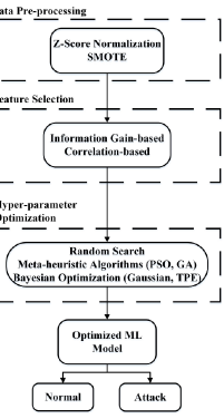
Figure 1: Proposed Multi-stage Optimized ML-based NIDS Framework

V Proposed Multi-Stage Optimized ML-based NIDS Framework

V-A General Framework Description:

This work focuses on building a multi-stage optimized ML-based NIDS framework that achieves high detection accuracy, low FAR, and has a low time complexity.The proposed framework is divided into three main stages to achieve this goal. The first stage includes the data pre-processing that includes performing Z-score normalization and Synthetic Minority Oversampling TEchnique (SMOTE). This is done to improve the performance of the training model and reduce the class-imbalance often observed in network traffic data [35]. In turn, this can reduce the training sample size since the ML model would have enough samples to understand the behavior of each class [36].
The second stage of the proposed framework is conducting a feature selection process to reduce the number of features needed for the ML classification model. This is done to reduce the time complexity of the classification model and consequently decrease its training time without sacrificing its performance [38]. With that in mind, two different methods are compared within this stage of the framework.
The third stage of the framework involves the optimization of the hyper-parameters of the different ML classification models considered. To that end, three different hyper-parameter tuning/optimization models are investigated, namely random search, meta-heuristic optimization algorithms including particle swarm optimization (PSO) and genetic algorithm (GA), and Bayesian Optimization (BO) algorithm. These models represent three different hyper-parameter tuning/optimization categories which are heuristics [47], meta-heuristics [61], and probabilistic global optimization [57] models respectively.
The results of these optimization stages are combined to build the optimized ML classification model for effective NIDS system that classifies new instances as either normal or attack instances. Figure 1 illustrates the different stages of the proposed framework.

V-B Security Considerations:

The proposed multi-stage optimized ML-based NIDS framework is a signature-based NIDS system. This is illustrated by the fact that the framework oversamples the minority class, which typically is the attack class in network traffic [27, 28]. Thus, the framework learns from the observed patterns of the known initiated attacks [27, 28]. However, it is worth noting that the framework can work as an anomaly-based NIDS since it is trained by adopting a binary classification model so that it can classify any anomalous behavior as an attack.
This framework can be deployed as one module within a more comprehensive security framework/policy that an individual or organization can adopt. This security framework/policy can include other mechanisms such as firewalls, deep packet inspection, user access control, and user authentication mechanisms [62][63]. This would offer a multi-layer secure framework that can preserve the privacy and security of the users’ data and information.

V-C Complexity:

To determine the time complexity of the proposed multi-stage optimized ML-based NIDS framework, we need to determine the complexity of each algorithm used in each stage. Given that this work compares the performance of different algorithms within the different stages of the framework, the overall time complexity is determined by the combination of algorithms that results in the highest aggregate complexity.
It is assumed that the data is composed of $M$ samples and $N$ features. Starting with the first stage, i.e. the data pre-processing stage, the complexity of the Z-score normalization process is $O(N)$ since we need to normalize all the samples of the $N$ features within the dataset. On the other hand, the complexity of the SMOTE algorithm is $O(M^{2}_{min}N)$ where $M_{min}$ is the number of samples belonging to the minority class [64]. Thus, the overall complexity of the first stage is $O(M^{2}_{min}N)$.
The complexity of the second stage is dependent on the complexity of the different feature selection algorithms considered. The complexity of Correlation-based feature selection is $O(MN^{2})$ since this method needs to calculate all the class-feature and feature-feature correlations [42]. In contrast, the complexity of the information gain-based feature selection method is $O(MN)$. This is due to the fact that this method has to calculate the joint probabilities of the class-feature interaction [40]. Therefore, the overall complexity of the second stage is $O(MN^{2})$.
Similarly, the complexity of the third stage depends on the complexity of each of the hyper-parameter optimization methods and the underlying ML model. Starting with the RS method, its complexity is $O(N_{parm}logN_{parm})$ where $N_{parm}$ is the number of parameters to be optimized [65]. Conversely, the complexity of the PSO algorithm is $O(N_{parm}N_{pop})$ where $N_{pop}$ is the population size, i.e. the number of swarm particles or potential solutions that we start with [66]. In a similar fashion, it can be shown that the complexity of the GA algorithm is also $O(N_{parm}N_{pop})$ where $N_{pop}$ is the population size, i.e. the number of chromosomes/potential solutions at the initialization stage [67]. For the GP-based BO algorithm, the complexity is $O(M^{3}_{red})$ where $M_{red}$ is the size of the reduced training sample. This is because the optimization process is carried on the training sample chosen after pre-processing and feature selection. In contrast, the time complexity of the TPE-based BO model is $O(M_{red}logM_{red})$ since this model follows a tree-like structure when performing the optimization [68].
Based on the aforementioned discussion, the overall complexity of the proposed framework is $O(MN^{2})$. This is because the second stage will dominate the complexity as it would still use the complete dataset rather than the reduced training dataset. As such, even if we consider the complexity of the potential ML classification model (for example the complexity of KNN classifier can be estimated as $O(M_{red}N_{red})$ [69, 70] where $N_{red}$ is the size of the reduced feature set), it is dependent on the reduced training sample dataset with reduced feature set size. Hence, the multi-stage optimized ML-based NIDS framework’s complexity is $O(MN^{2})$. Determining the overall time complexity of the complete framework including the optimized ML model training is essential since the model will be frequently re-trained to learn new attack patterns. This is based on the fact that network intrusion attacks continue to evolve and thus organizations need to have a flexible and dynamic NIDSs to keep up with these new attacks.

VI Datasets Description

This work uses two state-of-the-art intrusion datasets to evaluate the performance of the proposed multi-stage optimized ML-based NIDS framework. In what follows, a brief description of the two datasets is given.

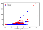
Figure 2: Principal Component Analysis of CICIDS 2017 Dataset Illustrating its Non-linear Nature

VI-A CICIDS 2017

The first dataset under consideration is the Canadian Institute of Cybersecurity’s IDS 2017 (CICIDS2017) dataset [12]. This dataset is an extension of the ISCX 2012 dataset used in our previous work [11]. The dataset was generated with the goal of it resembling realistic background traffic [12]. As such, the dataset contains benign and 14 of the most up-to-date common network attacks. The data collection process span a duration of five days from Monday July 3 till Friday July 7, 2017. Within this period, different attacks where generated during different time windows. The resulting dataset contained 3,119,345 instances and 83 features (1 class feature and 82 statistical features) representing the different characteristics of a network traffic request such as duration, protocol used, packet size, as well as source and destination details. However, nearly 300,000 samples were unlabeled and hence were discarded. Therefore, the refined dataset considered in this work contains 2,830,540 instances in total with 2,359,087 being BENIGN and 471,453 being ATTACK. Note that the attack instances represent various types of real-world network traffic attacks such as denial-of-service (DoS) and port scanning. However, this work merged all attacks into one label as the goal is to detect an attack regardless of its nature.
Fig. 2 shows the first and second principal components for the CICIDS 2017 dataset. It can be seen that the two classes are intertwined. Moreover, it can be observed that the features of the dataset are non-linear. Hence, we would expect a non-linear kernel to perform better in classifying the instances of this dataset.

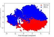
Figure 3: Principal Component Analysis of UNSW-NB 2015 Dataset Illustrating its Non-linear Nature

VI-B UNSW-NB 2015

The second dataset considered is the University of New South Wales’s network intrusion dataset (UNSW-NB 2015) generated in 2015 [14]. The dataset is a hybrid of real modern network normal activities and synthetic attack behaviors [14]. The data was collected through two different simulations conducted on two different days, namely January 22 and February 17, 2015. The resulting dataset consists of 2,540,044 instances and 49 features (1 class feature and 48 statistical features) representing the different characteristics of a network traffic request such as source and destination details, duration, protocol used, and packet size [14]. These instances are labeled as follows: 2,218,761 normal instances and 521,283 attack instances. In this case, no merging of attacks was needed since the dataset was originally labeled in a binary fashion.
In a similar fashion, Fig. 3 shows the first and second principal components for the UNSW-NB 2015 dataset. Again, we can observe that the features are non-linear. However, it can be observed that the level of intertwining between the two classes is lower. Accordingly, it is easier to separate between the two classes.
Note that there are other network intrusion detection datasets that can be studied such as the NSL KDD 99 dataset and the Kyoto 2006+ datasets. However, these datasets have already been extensively studied. Moreover, they are outdated and may not have recent attack patterns. In contrast, the two datasets considered in this work are more recent and have more attack patterns. As such, studying them will provide better equipped NIDSs that are trained to detect more attack types.

VI-C Attack Types

The two datasets considered in this work contain some similar attacks and some that are different. For example, the CICIDS 2017 dataset contains the following attacks: Denial-of-Service (DoS), port scanning, brute-force, web-attacks, botnets, and infiltration [12]. In contrast, the UNSW-NB 2015 dataset contains the following attacks: fuzzers, analysis, backdoors, DoS, exploits, generic, reconnaissance, shellcode, and worms [14]. Accordingly, it can be deduced that the proposed framework learns the patterns of various attack types.
Note that the proposed framework adopts a binary classification model by labeling all attack types as “attack”. The goal is to develop a NIDS that can detect various attacks rather than just a finite group of common attacks such as DoS. This reiterates the idea that the proposed multi-stage optimized ML-based NIDS can work as an anomaly-based NIDS despite its training as a signature-based NIDS.

VII Experimental Performance Evaluation

VII-A Experimental Setup

The experiments conducted for this work were completed using Python 3.7.4 running on Anaconda’s Jupyter Notebook. This was run on a virtual machine having a 3 processors Intel (R) Xeon (R) CPU E5-2660 v3 2.6 GHz and 64GB of memory running Windows Server 2016. The experimental results are divided into three main subsections, namely the impact of data pre-processing on training sample size, impact of feature selection on feature set size and training sample size, and the impact of optimization methods on the ML models’ detection performance.
The classification models used in this work are KNN classifier and the RF classifier. These classifiers were chosen due to two main reasons. Firstly, these classifiers were the top performing classifiers in our previous work as they showed their effectiveness with network intrusion detection [11]. Secondly, these classifiers have lower computational complexities when compared to other classifiers. For example, the KNN classifier has a complexity of $O(MN)$ where $M$ is the number of instances and $N$ is the number of features [69, 70]. Similarly, the complexity of the RF classifier is $O(M^{2}\sqrt{N}t)$ where $t$ is the number of trees within the RF classifier. However, since this classifier allows for multi-threading, its training time is significantly reduced to approximately $O(\frac{N^{2}\sqrt{M}t}{threads})$ where $threads$ is the maximum number of participating threads [30]. In contrast, the complexity of SVM can reach an order of $O(M^{3}N)$ [71]. Therefore, training such a model would be computationally prohibitive, especially given the dataset sizes used in this work. Note that the parameters to be tuned are:

• KNN: number of neighbors K.

• RF: Splitting criterion (Gini or Entropy) and Number of trees.

It is worth noting that the runtime complexity (also commonly referred to as testing complexity) of KNN and RF optimized models is $O(MN)$ and $O(Nt)$ respectively where $M$ is the number of training samples, $N$ is the number of features, and $t$ is the number of decision trees forming the RF classifier [72, 73]. In the case of KNN, any new instance is classified after calculating the distance between itself and all other instances in the training sample and identifying its K nearest neighbors [72]. Conversely, when using the RF classifier, the new instance is fed to the $t$ different decision trees, each of which uses $N$ splits based on the $N$ features considered, and the class is determined based on the majority vote among these $t$ trees.

VII-B Results and Discussion

VII-B1 Impact of data pre-processing on training sample size

Starting with the impact of data pre-processing stage on the training sample size, the learning curve showing the variation of training accuracy and the cross-validation accuracy as the training sample size changes. Both datasets were split randomly into training and testing samples after normalization using a 70%/30% split criterion.
Using the SMOTE technique, the number of instances of each type in each dataset’s training sample is as follows:

• CICIDS 2017: 1,818,477 benign instances (denoted as 0) and 1,800,000 attack instances (denoted as 1).

• UNSW-NB 2015: 1,775,010 normal instances (denoted as 0) and 1,500,000 attack instances (denoted as 1).

It can be seen from Fig. 4 that the number of training samples needed for the CICIDS 2017 dataset for the training accuracy and cross-validation accuracy to converge is close to 2.3 million samples. Similarly, for the UNSW-NB 2015 dataset, the number of training samples needed is close to 1.3 million samples as can be seen from Fig. 5. This can be attributed to the fact that both datasets are originally imbalanced with much fewer attack samples when compared to normal samples. Hence, the model struggles to learn the attack patterns and behaviors.

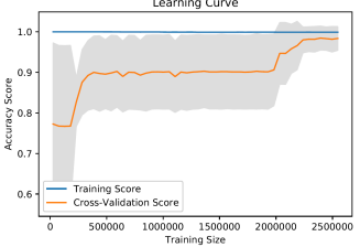
Figure 4: Learning Curve Showing Training and Cross-Validation Accuracy for CICIDS 2017 Dataset Before SMOTE

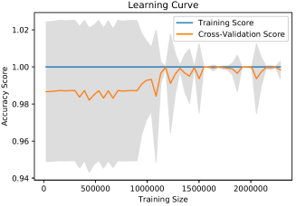
Figure 5: Learning Curve Showing Training and Cross-Validation Accuracy for UNSW-NB 2015 Dataset Before SMOTE

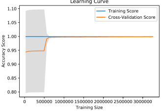
Figure 6: Learning Curve Showing Training and Cross-Validation Accuracy for CICIDS 2017 Dataset After SMOTE

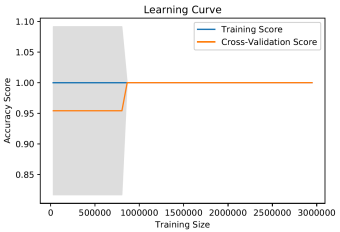
Figure 7: Learning Curve Showing Training and Cross-Validation Accuracy for UNSW-NB 2015 Dataset After SMOTE

In contrast, it can be seen from Figs. 6 and 7 that the number of training samples needed is around 600,000 samples and 800,000 samples for the CICIDS 2017 and UNSW-NB 2015 respectively. This represents a drop of approximately 74% and 39% in the training sample size for the two datasets respectively. This highlights the positive impact of using SMOTE technique as it was able to significantly reduce the size of the training sample needed without sacrificing the detection performance. This is mainly due to the introduction of more attack samples that allow the ML model to better learn their patterns and behaviors. To further highlight the impact of using data pre-processing phase, the time needed to build the learning curve was determined. For example, building the learning curve for the UNSW-NB 2015 dataset needed close to 600 minutes prior to applying SMOTE. In contrast, it required around 90 minutes after implementing SMOTE. This highlights the time complexity reduction associated with adopting an oversampling technique.
Moreover, it can be seen from all these figures that the models developed before and after SMOTE for both datasets do not suffer from overfitting as illustrated by the relatively small error gap between the training and cross-validation accuracy in Figs. 4 and 5 and the zero error gap seen in Figs. 6 and 7. As per [74], overfitting can be observed from the learning curve whenever the error gap between the training accuracy and the cross-validation accuracy is large. Thus, a small or zero error gap implies that the developed model is not too specific to the training dataset but can perform equally well on the testing and cross-validation sets.

Figure 8: Mutual Information Score of Features for CICIDS 2017 Dataset Showing the Highest Scoring Features in Descending Order

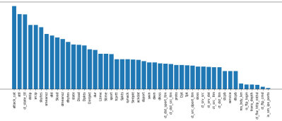
Figure 9: Mutual Information Score of Features for UNSW-NB 2015 Dataset Showing the Highest Scoring Features in Descending Order

VII-B2 Impact of feature selection on feature set size and training sample size

The second stage of analysis involves studying the impact of the different feature selection algorithms on the feature set size and training sample size.

1. Impact of feature selection on feature set size: Starting with the IGBFS method, Figs. 8 and 9 show the mutual information score for each of the features for the CICIDS 2017 and UNSW-NB 2015 datasets respectively. For example, for the CICIDS 2017 dataset, some of the most informative features include the average packet size and packet length variance. Similarly, for the UNSW-NB 2015 dataset, some of the most informative features are also the packet size (denoted by sbyte and dbyte features) and the time to live values. This illustrates the tendency of attacks to have different packet sizes when compared to normal traffic. Moreover, the figures also show that some IPs may have a higher tendency to initiate attacks, which means they are more likely to be compromised.
   Based on the figures, the number of features selected for the CICIDS 2017 and UNSW-NB 2015 datasets is 31 features and 19 features, respectively. This represents a reduction of 62% and 61% in the feature set size for the two datasets respectively. This is caused by the IGBFS method choosing the relevant features that provide the most information about the class.
   In contrast, when using the CBFS method, the number of selected features for the CICIDS 2017 and UNSW-NB 2015 datasets is 41 and 32 features respectively. This represents a reduction of 50% and 33.3% for each of the datasets, respectively. This reduction is due to the CBFS method choosing the relevant features that are highly correlated with the class feature, i.e. the features whose variation is also reflected in a variation in the corresponding class.
   The IGBFS method tends to choose a lower number of features when compared to the CBFS method. This is because the CBFS method relies on the correlation. Thus, two features may be chosen that are highly correlated with the class because they have a high correlation between them and one of them is highly correlated with the class. On the other hand, the IGBFS method studies the features one by one with respect to the class and selects the features that provide the highest amount of information about the class without considering the mutual information between the features themselves. Hence, a lower number of features is typically chosen by the IGBFS method.

2. Impact of feature selection on training sample size: In addition to the impact of the feature selection process on the feature set size, this work also studies its impact on the training sample size. Starting with the IGBFS method, it can be seen from Figs. 10 and 11 that the training sample size was reduced to 250,000 and 110,000 samples for the CICIDS 2017 and UNSW-NB 2015 datasets, respectively. This represents a reduction of 59% and 86% when compared to the required training sample size after the SMOTE technique is applied. This shows that the IGBFS method can keep the features that provide the most information about the class and discard any feature that may be negatively impacting the learning process.
   

   

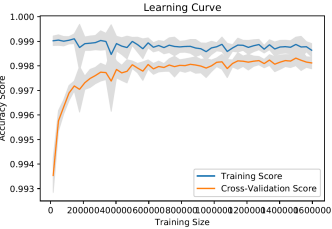
   Figure 10: Learning Curve Showing Training and Cross-Validation Accuracy for CICIDS 2017 Dataset After IGBFS

   

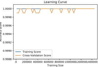
   Figure 11: Learning Curve Showing Training and Cross-Validation Accuracy for UNSW-NB 2015 Dataset After IGBFS

   

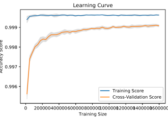
   Figure 12: Learning Curve Showing Training and Cross-Validation Accuracy for CICIDS 2017 Dataset After CBFS

   

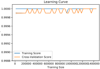
   Figure 13: Learning Curve Showing Training and Cross-Validation Accuracy for UNSW-NB 2015 Dataset After CBFS

Similarly for the case of using CBFS method, it can be observed from Figs. 12 and 13 that the required training sample size for the CICIDS 2017 and UNSW-NB 2015 datasets is reduced to 500,000 and 200,000, respectively. This represents a reduction of 17% and 75% when compared to the required training sample size after SMOTE technique is applied. This shows that the CBFS method is also able to select relevant features that have a positive impact on the learning process. However, since some of the features selected may be redundant, this may have a negative impact on the learning process when compared to that of the IGBFS. The time needed to build the learning curve using the two feature selection methods was determined to further highlight the impact of feature selection on the reduction of time complexity. For example, building the learning curve for the UNSW-NB 2015 dataset required around 21 minutes and 25 minutes for the IGBFS and CBFS methods, respectively. Accordingly, applying either of the two feature selection methods will have a positive impact on the feature set size and training sample size with the IGBFS method having a slight advantage over the CBFS method.
Figs. 10, 11, 12, and 13 describe a relatively small or zero error gap between the training accuracy and the cross-validation accuracy. This indicates that the model is suitable to be generalized for testing and cross-validation datasets and is not being overfit to the training dataset [74].

TABLE I: Optimal Parameter Values with IGBFS for Different ML Models

	CICIDS 2017	UNSW-NB 2015
Classifier	Parameter Values	Parameter Values
RS-KNN	Number of Neighbors= 3	Number of Neighbors= 11
PSO-KNN	Number of Neighbors= 5	Number of Neighbors= 11
GA-KNN	Number of Neighbors= 29	Number of Neighbors= 13
BO-GP-KNN	Number of Neighbors= 29	Number of Neighbors= 13
BO-TPE-KNN	Number of Neighbors= 29	Number of Neighbors= 13
RS-RF	Splitting Criterion= Gini, Number of trees= 40	Splitting Criterion= Entropy, Number of trees= 30
PSO-RF	Splitting Criterion= Gini, Number of trees= 21	Splitting Criterion= Entropy, Number of trees= 81
GA-RF	Splitting Criterion= Gini, Number of trees= 219	Splitting Criterion= Entropy, Number of trees= 168
BO-GP-RF	Splitting Criterion= Entropy, Number of trees= 200	Splitting Criterion= Entropy, Number of trees= 171
BO-TPE-RF	Splitting Criterion= Entropy, Number of trees= 90	Splitting Criterion= Entropy, Number of trees= 50

TABLE II: Optimal Parameter Values with CBFS for Different ML Models

	CICIDS 2017	UNSW-NB 2015
Classifier	Parameter Values	Parameter Values
RS-KNN	Number of Neighbors= 3	Number of Neighbors= 3
PSO-KNN	Number of Neighbors= 11	Number of Neighbors= 5
GA-KNN	Number of Neighbors= 25	Number of Neighbors= 25
BO-GP-KNN	Number of Neighbors= 29	Number of Neighbors= 25
BO-TPE-KNN	Number of Neighbors= 29	Number of Neighbors= 29
RS-RF	Splitting Criterion= Gini, Number of trees= 20	Splitting Criterion= Gini, Number of trees= 10
PSO-RF	Splitting Criterion= Gini, Number of trees= 87	Splitting Criterion= Gini, Number of trees= 54
GA-RF	Splitting Criterion= Gini, Number of trees= 219	Splitting Criterion= Gini, Number of trees= 219
BO-GP-RF	Splitting Criterion= Gini, Number of trees= 164	Splitting Criterion= Entropy, Number of trees= 78
BO-TPE-RF	Splitting Criterion= Entropy, Number of trees= 50	Splitting Criterion= Gini, Number of trees= 20

TABLE III: Performance Results of the Multi-stage Optimized ML-based NIDS Framework with IGBFS for Testing Datasets

	CICIDS 2017				UNSW-NB 2015
Classifier	Acc(%)	Precision	Recall	FAR	Acc(%)	Precision	Recall	FAR
RS-KNN	99.63%	0.99	0.99	0.001	99.96%	0.99	0.99	0.001
PSO-KNN	99.09%	0.98	0.99	0.001	99.91%	0.99	0.99	0.001
GA-KNN	99.09%	0.98	0.99	0.001	99.91%	0.99	0.99	0.001
BO-GP-KNN	99.11%	0.98	0.99	0.001	99.91%	0.99	0.99	0.001
BO-TPE-KNN	99.11%	0.98	0.99	0.001	99.91%	0.99	0.99	0.001
RS-RF	99.72%	0.99	0.99	0.001	100%	1.0	1.0	0.0
PSO-RF	99.98%	0.99	0.99	0.001	100%	1.0	1.0	0.0
GA-RF	99.98%	0.99	0.99	0.001	100%	1.0	1.0	0.0
BO-GP-RF	99.83%	0.99	0.99	0.001	100%	1.0	1.0	0.0
BO-TPE-RF	99.99%	0.99	0.99	0.001	100%	1.0	1.0	0.0

TABLE IV: Performance results of the Multi-stage Optimized ML-based NIDS Framework with CBFS for Testing Datasets

	CICIDS 2017				UNSW-NB 2015
Classifier	Acc(%)	Precision	Recall	FAR	Acc(%)	Precision	Recall	FAR
RS-KNN	99.70%	0.99	0.99	0.001	99.96%	0.99	0.99	0.001
PSO-KNN	99.28%	0.99	0.99	0.001	99.88%	0.99	0.99	0.001
GA-KNN	99.28%	0.99	0.99	0.001	99.88%	0.99	0.99	0.001
BO-GP-KNN	99.23%	0.99	0.99	0.001	99.88%	0.99	0.99	0.001
BO-TPE-KNN	99.23%	0.99	0.99	0.001	99.88%	0.99	0.99	0.001
RS-RF	99.61%	0.99	0.99	0.001	100%	1.0	1.0	0.0
PSO-RF	99.88%	0.99	0.99	0.001	100%	1.0	1.0	0.0
GA-RF	99.88%	0.99	0.99	0.001	100%	1.0	1.0	0.0
BO-GP-RF	99.88%	0.99	0.99	0.001	100%	1.0	1.0	0.0
BO-TPE-RF	99.99%	0.99	0.99	0.001	100%	1.0	1.0	0.0

VII-B3 Impact of optimization methods on the ML models’ detection performance

To evaluate the performance of the different classifiers and study the impact of the different optimization methods on them, we determine four evaluation metrics, namely the accuracy (acc), precision, recall/true positive rate (TPR), and false alarm/positive rate (FAR/FPR) as per [11][75] using the following equations:

$$Acc=\frac{tp+tn}{tp+tn+fp+fn}$$ (11)

$$Precision=\frac{tp}{tp+fp}$$ (12)

$$Recall/TPR=\frac{tp}{tp+fn}$$ (13)

$$FAR/FPR=\frac{fp}{tn+fp}$$ (14)

where $tp$ is the number of true positives, $tn$ is the number of true negatives, $fp$ is the number of false positives, and $fn$ is the number of false negatives. These values compose the confusion matrix of any ML model.
Table I gives the optimal parameter values for the two different classifiers when the IGBFS technique is used. In the case of KNN method, the RS and PSO methods tend to choose smaller values for the number of neighbors when compared to the GA, BO-GP, and BO-TPE methods. For the RS method, this is due to the fact that the algorithm’s stopping criterion is typically the number of iterations and thereby does not test all potential values. Accordingly, it is possible for it to miss the optimal number of neighbors. Similarly, one of the stopping criteria in the PSO algorithm is also the number of evaluations, which can also lead to it missing the optimal value. In contrast, the GA, BO-GP, and BO-TPE all resulted in a similar number of neighbors for both the CICIDS 2017 and UNSW-NB 2015 datasets. For the GA algorithm, the number of generations is typically set sufficiently high to reach the optimal value for the number of neighbors. In a similar manner, the BO-GP and BO-TPE determine the actual optimal value based on the assumed model.
In the case of the RF method, the RS and PSO algorithms tend to choose a lower number of trees compared to the GA, BO-GP, and BO-TPE. This is due to the algorithms’ stopping criterion that often leads to a pre-mature stoppage. In contrast, the GA, BO-GP, and BO-TPE determine that the number of trees needed is higher as they explore more potential values, allowing them to select more optimal values for the number of trees. In terms of the splitting criterion, the entropy criterion is mostly selected. This is expected since the IGBFS method selects features based on their information gain, which is determined using the entropy of each feature. As such, this criterion would be more suitable when using IGBFS.
Looking at Table II, similar observations about the hyper-parameter optimization performance of the different algorithms can be made for both the KNN and RF methods. The only difference is that for the RF method, the splitting criterion is chosen to be the Gini index. This is due to the CBFS method using the correlation as the selection criterion rather than the entropy. Therefore, the features chosen may result in a low amount of information (equivalent to having a high entropy with respect to the class), and thus would be overlooked if the entropy splitting criterion is chosen. This is the reason behind choosing the Gini splitting criterion when the CBFS method is used.
Tables III and IV show the performance of the two classification algorithms when using IGBFS and CBFS methods, respectively. Several observations can be made. The first observation is that the optimized models outperform the regular models recently reported in [12][30][76] by 1-2% on average in terms of accuracy and a reduction of 1-2% in FAR for both datasets. This is expected since one of the main goals of hyper-parameter optimization is to improve the performance of the ML models. The second observation is that the RF classifier outperforms the KNN classifier for both the IGBFS and CBFS methods as seen in the CICIDS 2017 and UNSW-NB 2015 datasets. This reiterates the previously obtained results in [11] with ISCX 2012 dataset and the reported results in [12][30][76] in which the RF classifier also outperformed the KNN model. This can be attributed to the RF classifier being an ensemble model. Accordingly, it is effective with non-linear and high-dimensional datasets like the datasets under consideration in this work. The third observation is that the BO-TPE-RF method had the highest detection accuracy for both the CICIDS 2017 and UNSW-NB 2015 datasets for both feature selection algorithms with a detection accuracy of 99.99% and 100%, respectively. This proves the effectiveness and robustness of the proposed multi-stage optimized ML-based NIDS framework as it outperformed other NIDS frameworks.

VIII Conclusion

The area of cyber-security has garnered significant attention from both the industry and academia due to the increased dependency of individuals and organizations on the Internet and their concern about the security and privacy of their activities. More resources are being deployed and allocated to protect modern Internet-based networks against potential attacks or anomalous activities. Accordingly, different types of network intrusion detection systems (NIDSs) have been proposed in the literature. Despite the continuous improvements in NIDS performance, there is still room for further improvement. More insights can be extracted from the high volume of network traffic data generated, the continuously changing environments, the plethora of features collected as part of training datasets (high dimensional datasets), and the need for real-time intrusion detection.
Choosing the most suitable subset of features and optimizing the parameters of the machine learning (ML)-based detection models is essential to enhance their performance. Accordingly, this paper expanded on our previous work by proposing a multi-stage optimized ML-based NIDS framework that reduced the computational complexity while maintaining its detection performance. Using two recent state-of-the-art intrusion detection datasets (CICIDS 2017 dataset and the UNSW-NB 2015 dataset) for performance evaluation, this work first studied the impact of oversampling techniques on the models’ training sample size and determined the minimum suitable training size for effective intrusion detection. Experimental results showed that using the SMOTE oversampling technique can reduce the training sample size between 39% and 74% of the original datasets’ size. Additionally, this work compared between two different feature selection techniques, namely information gain (IGBFS) and correlation-based feature selection (CBFS), and explored their impact on the feature set size, the training sample size, and the models’ detection performance. The experimental results showed that the feature selection methods were able to reduce the feature set size by almost 60%. Moreover, they further reduced the required training sample size between 33% and 50% when compared to the training sample after SMOTE. Finally, this work investigated the impact of different ML hyper-parameter optimization techniques on the NIDS’s performance using two ML classification models, namely the K-nearest neighbors (KNN) and the Random Forest (RF) classifiers. Experimental results showed that the optimized RF classifier with Bayesian Optimization using Tree Parzen Estimator (BO-TPE-RF) had the highest detection accuracy when compared to the other optimization techniques (enhanced the detection accuracy by 1-2% and reduce the FAR by 1-2% when compared to recent works from the literature). It was also observed that using the IGBFS method achieved better detection accuracy when compared to the CBFS method.
Other models such as deep learning classifiers can be explored for future work since these models perform admirably on non-linear and high-dimensional datasets. Investigating the impact of combining supervised and unsupervised ML techniques may also prove paramount in this field to detect novel attacks.

MohammadNoor Injadat received the B.Sc. and M.Sc. degrees in Computer Science from Al Al-Bayt University and University Putra Malaysia in Jordan and Malaysia in 2000 and 2002, respectively. He obtained a Master of Engineering in Electrical and Computer Engineering from University of Western Ontario in 2015. He obtained his Ph.D. degree in Software Engineering at the Department of Electrical and Computer Engineering, University of Western Ontario in Canada in 2020. His research interests include data mining, machine learning, social network analysis, e-learning analytics, and network security.

Abdallah Moubayed received his Ph.D. in Electrical & Computer Engineering from the University of Western Ontario in August 2018, his M.Sc. degree in Electrical Engineering from King Abdullah University of Science and Technology, Thuwal, Saudi Arabia in 2014, and his B.E. degree in Electrical Engineering from the Lebanese American University, Beirut, Lebanon in 2012. Currently, he is a Postdoctoral Associate in the Optimized Computing and Communications (OC2) lab at University of Western Ontario. His research interests include wireless communication, resource allocation, wireless network virtualization, performance & optimization modeling, machine learning & data analytics, computer network security, cloud computing, and e-learning.

Ali Bou Nassif received his Ph.D. degree in Electrical and Computer engineering from The University of Western Ontario, London, Ontario, Canada (2012). He is currently an Assistant Professor and an Assistant Dean of the Graduate Studies, University of Sharjah, United Arab Emirates, and an Adjunct Research Professor with Western University. He has published more than 60 papers in international journals and conferences. His interests are Machine Learning and Soft Computing, Software Engineering, Cloud Computing and Service Oriented Architecture (SOA), and Mobile Computing. Ali is a registered professional engineer in Ontario, as well as a member of IEEE Computer Society.

Abdallah Shami is a Professor at the ECE department at Western University, Ontario, Canada. Dr. Shami is the Director of the Optimized Computing and Communications Laboratory at Western. He is currently an Associate Editor for IEEE Transactions on Mobile Computing, IEEE Network, and IEEE Communications Tutorials and Survey. Dr. Shami has chaired key symposia for IEEE GLOBECOM, IEEE ICC, IEEE ICNC, and ICCIT. He was the elected Chair of the IEEE Communications Society Technical Committee on Communications Software (2016-2017) and IEEE London Ontario Section Chair (2016-2018).

References

- [1] C.-F. Tsai, Y.-F. Hsu, C.-Y. Lin, and W.-Y. Lin, “Intrusion detection by machine learning: A review,” Expert Systems with Applications, vol. 36, no. 10, pp. 11 994–12 000, 2009.
- [2] A. Moubayed, M. Injadat, A. Shami, and H. Lutfiyya, “Student engagement level in e learning environment: Clustering using k-means,” American Journal of Distance Education, vol. 34, no. 2, 2019.
- [3] M. Injadat, F. Salo, and A. B. Nassif, “Data mining techniques in social media: A survey,” Neurocomputing, vol. 214, pp. 654 – 670, 2016. [Online]. Available: http://www.sciencedirect.com/science/article/pii/S092523121630683X
- [4] M. B. Salem, S. Hershkop, and S. J. Stolfo, “A survey of insider attack detection research,” in Insider Attack and Cyber Security. Springer, 2008, pp. 69–90.
- [5] W. Bul’ajoul, A. James, and M. Pannu, “Improving network intrusion detection system performance through quality of service configuration and parallel technology,” Journal of Computer and System Sciences, vol. 81, no. 6, pp. 981–999, 2015.
- [6] S. M. H. Bamakan, B. Amiri, M. Mirzabagheri, and Y. Shi, “A new intrusion detection approach using pso based multiple criteria linear programming,” Procedia Computer Science, vol. 55, pp. 231–237, 2015.
- [7] S. X. Wu and W. Banzhaf, “The use of computational intelligence in intrusion detection systems: A review,” Applied soft computing, vol. 10, no. 1, pp. 1–35, 2010.
- [8] H.-J. Liao, C.-H. R. Lin, Y.-C. Lin, and K.-Y. Tung, “Intrusion detection system: A comprehensive review,” Journal of Network and Computer Applications, vol. 36, no. 1, pp. 16–24, 2013.
- [9] S. Suthaharan, “Big data classification: Problems and challenges in network intrusion prediction with machine learning,” ACM SIGMETRICS Performance Evaluation Review, vol. 41, no. 4, pp. 70–73, 2014.
- [10] J. Zhang and M. Zulkernine, “Anomaly based network intrusion detection with unsupervised outlier detection,” in Communications, 2006. ICC’06. IEEE International Conference on, vol. 5. IEEE, 2006, pp. 2388–2393.
- [11] M. Injadat, F. Salo, A. B. Nassif, A. Essex, and A. Shami, “Bayesian optimization with machine learning algorithms towards anomaly detection,” in 2018 IEEE Global Communications Conference (GLOBECOM), 2018, pp. 1–6.
- [12] I. Sharafaldin, A. H. Lashkari, and A. A. Ghorbani, “Toward generating a new intrusion detection dataset and intrusion traffic characterization.” in ICISSP, 2018, pp. 108–116.
- [13] A. Shiravi, H. Shiravi, M. Tavallaee, and A. A. Ghorbani, “Toward developing a systematic approach to generate benchmark datasets for intrusion detection,” Computers and Security, vol. 31, no. 3, pp. 357 – 374, 2012.
- [14] N. Moustafa and J. Slay, “Unsw-nb15: a comprehensive data set for network intrusion detection systems (unsw-nb15 network data set),” in 2015 Military Communications and Information Systems Conference (MilCIS), Nov. 2015, pp. 1–6.
- [15] F. Kuang, W. Xu, and S. Zhang, “A novel hybrid kpca and svm with ga model for intrusion detection,” Applied Soft Computing, vol. 18, pp. 178–184, 2014.
- [16] A. S. Eesa, Z. Orman, and A. M. A. Brifcani, “A novel feature-selection approach based on the cuttlefish optimization algorithm for intrusion detection systems,” Expert Systems with Applications, vol. 42, no. 5, pp. 2670–2679, 2015.
- [17] W. Li, P. Yi, Y. Wu, L. Pan, and J. Li, “A new intrusion detection system based on knn classification algorithm in wireless sensor network,” Journal of Electrical and Computer Engineering, vol. 2014, 2014.
- [18] A. B. Nassif, L. F. Capretz, and D. Ho, “Estimating software effort using an ann model based on use case points,” in 2012 11th International Conference on Machine Learning and Applications, vol. 2, 2012, pp. 42–47.
- [19] A. Moubayed, M. Injadat, A. B. Nassif, H. Lutfiyya, and A. Shami, “E-learning: Challenges and research opportunities using machine learning data analytics,” IEEE Access, vol. 6, pp. 39 117–39 138, 2018.
- [20] S. Aljawarneh, M. Aldwairi, and M. B. Yassein, “Anomaly-based intrusion detection system through feature selection analysis and building hybrid efficient model,” Journal of Computational Science, 2017.
- [21] A. Moubayed, M. Injadat, A. Shami, and H. Lutfiyya, “Dns typo-squatting domain detection: A data analytics and machine learning based approach,” in 2018 IEEE Global Communications Conference (GLOBECOM). IEEE, 2018, pp. 1–7.
- [22] A. Moubayed, E. Aqeeli, and A. Shami, “Ensemble-based Feature Selection and Classification Model for DNS Typo-squatting Detection,” in Accepted in 33rd Canadian Conference on Electrical and Computer Engineering (CCECE’20. IEEE, 2020, pp. 1–6.
- [23] X. Sun, J. Dai, P. Liu, A. Singhal, and J. Yen, “Using bayesian networks for probabilistic identification of zero-day attack paths,” IEEE Transactions on Information Forensics and Security, vol. 13, no. 10, pp. 2506–2521, Oct. 2018.
- [24] A. Alsirhani, S. Sampalli, and P. Bodorik, “Ddos detection system: Using a set of classification algorithms controlled by fuzzy logic system in apache spark,” IEEE Transactions on Network and Service Management, vol. 16, no. 3, pp. 936–949, Sep. 2019.
- [25] A. A. Daya, M. A. Salahuddin, N. Limam, and R. Boutaba, “Botchase: Graph-based bot detection using machine learning,” IEEE Transactions on Network and Service Management, pp. 1–1, 2020.
- [26] T. Kim, B. Kang, M. Rho, S. Sezer, and E. G. Im, “A multimodal deep learning method for android malware detection using various features,” IEEE Transactions on Information Forensics and Security, vol. 14, no. 3, pp. 773–788, Mar. 2019.
- [27] F. Salo, M. Injadat, A. B. Nassif, A. Shami, and A. Essex, “Data mining techniques in intrusion detection systems: A systematic literature review,” IEEE Access, vol. 6, pp. 56 046–56 058, 2018.
- [28] F. Salo, M. Injadat, A. B. Nassif, and A. Essex, “Data mining with big data in intrusion detection systems: A systematic literature review,” in International Symposium on Big Data Management and Analytics 2019, Apr. 2019.
- [29] F. Salo, M. Injadat, A. Moubayed, A. B. Nassif, and A. Essex, “Clustering enabled classification using ensemble feature selection for intrusion detection,” in 2019 International Conference on Computing, Networking and Communications (ICNC). IEEE, 2019, pp. 276–281.
- [30] L. Yang, A. Moubayed, I. Hamieh, and A. Shami, “Tree-based intelligent intrusion detection system in internet of vehicles,” in 2019 IEEE Global Communications Conference (GLOBECOM), 2019.
- [31] Y. Y. Chung and N. Wahid, “A hybrid network intrusion detection system using simplified swarm optimization (sso),” Applied Soft Computing, vol. 12, no. 9, pp. 3014–3022, 2012.
- [32] F. Kuang, W. Xu, and S. Zhang, “A novel hybrid kpca and svm with ga model for intrusion detection,” Applied Soft Computing, vol. 18, pp. 178–184, 2014.
- [33] J. Zhang, M. Zulkernine, and A. Haque, “Random-forests-based network intrusion detection systems,” IEEE Transactions on Systems, Man, and Cybernetics, Part C (Applications and Reviews), vol. 38, no. 5, pp. 649–659, 2008.
- [34] K. M. Ali Alheeti and K. McDonald-Maier, “Intelligent intrusion detection in external communication systems for autonomous vehicles,” Systems Science and Control Engineering, vol. 6, no. 1, pp. 48–56, 2018.
- [35] Z. Chen, Q. Yan, H. Han, S. Wang, L. Peng, L. Wang, and B. Yang, “Machine learning based mobile malware detection using highly imbalanced network traffic,” Information Sciences, vol. 433, pp. 346–364, 2018.
- [36] N. V. Chawla, K. W. Bowyer, L. O. Hall, and W. P. Kegelmeyer, “Smote: synthetic minority over-sampling technique,” Journal of artificial intelligence research, vol. 16, pp. 321–357, 2002.
- [37] X. Tan, S. Su, Z. Huang, X. Guo, Z. Zuo, X. Sun, and L. Li, “Wireless sensor networks intrusion detection based on smote and the random forest algorithm,” Sensors, vol. 19, no. 1, p. 203, 2019.
- [38] M. B. Çatalkaya, O. Kalıpsız, M. S. Aktaş, and U. O. Turgut, “Data feature selection methods on distributed big data processing platforms,” in 2018 3rd International Conference on Computer Science and Engineering (UBMK), Sep. 2018, pp. 133–138.
- [39] R. S. B. Krishna and M. Aramudhan, “Feature Selection Based on Information Theory for Pattern Classification,” in 2014 International Conference on Control, Instrumentation, Communication and Computational Technologies (ICCICCT), Jul. 2014, pp. 1233–1236.
- [40] B. Bonev, “Feature selection based on information theory,” Ph.D. dissertation, University of Alicante, Jun. 2010.
- [41] J. Li, K. Cheng, S. Wang, F. Morstatter, R. P. Trevino, J. Tang, and H. Liu, “Feature selection: A data perspective,” ACM Computing Surveys (CSUR), vol. 50, no. 6, p. 94, 2018.
- [42] M. A. Hall, “Correlation-based feature selection for machine learning,” Ph.D. dissertation, University of Waikato Hamilton, 1999.
- [43] A. Moubayed, M. Injadat, A. Shami, and H. Lutfiyya, “Relationship between student engagement and performance in e learning environment using association rules,” in 2018 IEEE World Engineering Education Conference (EDUNINE), Mar. 2018, pp. 1–6.
- [44] J. H. Gennari, P. Langley, and D. Fisher, “Models of incremental concept formation,” Artificial intelligence, vol. 40, no. 1-3, pp. 11–61, 1989.
- [45] P. Koch, B. Wujek, O. Golovidov, and S. Gardner, “Automated hyperparameter tuning for effective machine learning,” in Proceedings of the SAS Global Forum 2017 Conference, 2017, pp. 1–23.
- [46] L. Yang and A. Shami, “On hyperparameter optimization of machine learning algorithms: Theory and practice,” Neurocomputing, 2020. [Online]. Available: http://www.sciencedirect.com/science/article/pii/S0925231220311693
- [47] J. Bergstra and Y. Bengio, “Random search for hyper-parameter optimization,” Journal of machine learning research, vol. 13, no. Feb, pp. 281–305, 2012.
- [48] M. Injadat, A. Moubayed, A. B. Nassif, and A. Shami, “Systematic ensemble model selection approach for educational data mining,” Knowledge-Based Systems, vol. 200, p. 105992, 2020. [Online]. Available: http://www.sciencedirect.com/science/article/pii/S0950705120302999
- [49] ——, “Multi-split Optimized Bagging Ensemble Model Selection for Multi-class Educational Datasets,” Applied Intelligence, 2020.
- [50] L. Bianchi, M. Dorigo, L. M. Gambardella, and W. J. Gutjahr, “A survey on metaheuristics for stochastic combinatorial optimization,” Natural Computing, vol. 8, no. 2, pp. 239–287, 2009.
- [51] S.-W. Lin, K.-C. Ying, S.-C. Chen, and Z.-J. Lee, “Particle swarm optimization for parameter determination and feature selection of support vector machines,” Expert Systems with Applications, vol. 35, no. 4, pp. 1817 – 1824, 2008.
- [52] G. Cohen, M. Hilario, and A. Geissbuhler, “Model selection for support vector classifiers via genetic algorithms. an application to medical decision support,” in International Symposium on Biological and Medical Data Analysis. Springer, 2004, pp. 200–211.
- [53] S. G. Ahmad, C. S. Liew, E. U. Munir, T. F. Ang, and S. U. Khan, “A hybrid genetic algorithm for optimization of scheduling workflow applications in heterogeneous computing systems,” Journal of Parallel and Distributed Computing, vol. 87, pp. 80–90, 2016.
- [54] S. Blaifi, S. Moulahoum, I. Colak, and W. Merrouche, “An enhanced dynamic model of battery using genetic algorithm suitable for photovoltaic applications,” Applied Energy, vol. 169, pp. 888–898, 2016.
- [55] U. Mehboob, J. Qadir, S. Ali, and A. Vasilakos, “Genetic algorithms in wireless networking: techniques, applications, and issues,” Soft Computing, vol. 20, no. 6, pp. 2467–2501, 2016.
- [56] A. Rikhtegar, M. Pooyan, and M. T. Manzuri-Shalmani, “Genetic algorithm-optimised structure of convolutional neural network for face recognition applications,” IET Computer Vision, vol. 10, no. 6, pp. 559–566, 2016.
- [57] J. Snoek, H. Larochelle, and R. P. Adams, “Practical bayesian optimization of machine learning algorithms,” in Advances in neural information processing systems, 2012, pp. 2951–2959.
- [58] E. Brochu, V. M. Cora, and N. De Freitas, “A tutorial on bayesian optimization of expensive cost functions, with application to active user modeling and hierarchical reinforcement learning,” arXiv preprint arXiv:1012.2599, 2010.
- [59] I. Dewancker, M. McCourt, and S. Clark, “Bayesian optimization primer,” 2015.
- [60] K. Eggensperger, M. Feurer, F. Hutter, J. Bergstra, J. Snoek, H. Hoos, and K. Leyton-Brown, “Towards an empirical foundation for assessing bayesian optimization of hyperparameters,” in NIPS workshop on Bayesian Optimization in Theory and Practice, vol. 10, 2013, p. 3.
- [61] D. Ashlock, Evolutionary computation for modeling and optimization. Springer Science and Business Media, 2006.
- [62] A. Moubayed, A. Refaey, and A. Shami, “Software-defined perimeter (sdp): State of the art secure solution for modern networks,” IEEE Network, vol. 33, no. 5, pp. 226–233, 2019.
- [63] P. Kumar, A. Moubayed, A. Refaey, A. Shami, and J. Koilpillai, “Performance analysis of sdp for secure internal enterprises,” in 2019 IEEE Wireless Communications and Networking Conference (WCNC), 2019, pp. 1–6.
- [64] F. Hu and H. Li, “A novel boundary oversampling algorithm based on neighborhood rough set model: Nrsboundary-smote,” Mathematical Problems in Engineering, vol. 2013, 2013.
- [65] A. Lissovoi, P. S. Oliveto, and J. A. Warwicker, “On the time complexity of algorithm selection hyper-heuristics for multimodal optimisation,” in Proceedings of the AAAI Conference on Artificial Intelligence, vol. 33, 2019, pp. 2322–2329.
- [66] R. Cheng and Y. Jin, “A social learning particle swarm optimization algorithm for scalable optimization,” Information Sciences, vol. 291, pp. 43–60, 2015.
- [67] P. S. Oliveto and C. Witt, “Improved time complexity analysis of the simple genetic algorithm,” Theoretical Computer Science, vol. 605, pp. 21–41, 2015.
- [68] M. Feurer and F. Hutter, “Hyperparameter optimization,” in Automated Machine Learning. Springer, 2019, pp. 3–33.
- [69] The Kernel Trip, “Computational complexity of machine learning algorithms,” Apr. 2018.
- [70] C.-T. Chu, S. K. Kim, Y.-A. Lin, Y. Yu, G. Bradski, K. Olukotun, and A. Y. Ng, “Map-reduce for machine learning on multicore,” in Advances in neural information processing systems, 2007, pp. 281–288.
- [71] F. Pedregosa, G. Varoquaux, A. Gramfort, V. Michel, B. Thirion, O. Grisel, M. Blondel, P. Prettenhofer, R. Weiss, V. Dubourg, J. Vanderplas, A. Passos, D. Cournapeau, M. Brucher, M. Perrot, and E. Duchesnay, “Scikit-learn: Machine learning in Python,” Journal of Machine Learning Research, vol. 12, pp. 2825–2830, 2011.
- [72] O. Veksler, “Cs434a/541a class notes prof. olga veksler,” 2015. [Online]. Available: http://www.csd.uwo.ca/courses/CS9840a/Lecture2_knn.pdf
- [73] X. Solé, A. Ramisa, and C. Torras, “Evaluation of random forests on large-scale classification problems using a bag-of-visual-words representation.” in CCIA, 2014, pp. 273–276.
- [74] G. James, D. Witten, T. Hastie, and R. Tibshirani, An introduction to statistical learning. Springer, 2013, vol. 112.
- [75] A. B. Nassif, D. Ho, and L. F. Capretz, “Regression model for software effort estimation based on the use case point method,” in 2011 International Conference on Computer and Software Modeling, vol. 14, 2011, pp. 106–110.
- [76] N. Moustafa, B. Turnbull, and K. R. Choo, “An ensemble intrusion detection technique based on proposed statistical flow features for protecting network traffic of internet of things,” IEEE Internet of Things Journal, vol. 6, no. 3, pp. 4815–4830, 2019.