Algebraic and symplectic viewpoint on compactifications of two-dimensional cluster varieties of finite type

Abstract

In this article we explore compactifications of cluster varieties of finite type in complex dimension two. Cluster varieties can be viewed as the spec of a ring generated by theta functions and a compactification of such varieties can be given by a grading on that ring, which can be described by positive polytopes ghkk . In the examples we explore, the cluster variety can be interpreted as the complement of certain divisors in del Pezzo surfaces. In the symplectic viewpoint, they can be described via almost toric fibrations over $\mathbb{R}^{2}$ (after completion). Once identifying them as almost toric manifolds, one can symplectically view them inside other del Pezzo surfaces. So we can identify other symplectic compactifications of the same cluster variety, which we expect should also correspond to different algebraic compactifications. Both viewpoints are presented here and several compactifications have their corresponding polytopes compared. The finiteness of the cluster mutations are explored to provide cycles in the graph describing monotone Lagrangian tori in del Pezzo surfaces connected via almost toric mutation Vi16a .

1 Introduction

Cluster algebras, introduced by Fomin and Zelevinsky cluster1 , are subalgebras of rational functions in $n$ variables. The generators of cluster algebras are called the cluster variables. Instead of being given the complete sets of generators and relations as other commutative rings, a cluster algebra is defined from an (initial) seed, which includes a set of the generators and a matrix. An iterative procedure called mutation would produce new seeds from a given seed and this process gives all the cluster variables. The cluster algebra is then defined to be the ring generated by all cluster variables.

Geometrically, the cluster varieties, described by Fock and Goncharov FGdilog1 , and by Gross, Hacking, Keel in GHK_bir , are defined in a similar manner. A seed data now would be associated to an algebraic torus. The mutation procedures give the birational transformations used to glue the tori. A cluster variety is then the union of the tori under the gluing.

The compactification of the cluster varieties can be given by a Rees construction. Combinatorially, the construction can be described by ‘convex’ polytopes, called the positive polytopes ghkk . The article cpt showed that the positive polytopes satisfy a convexity condition called ‘broken line convexity’. As the seed mutates, the polytope mutates correspondingly. One can then give a mutation process to the polytopes. Note that under this type of mutation, there is no change in the compactification.

More generally, one can similarly describe the compactification of the log Calabi-Yau surfaces studied in GHKlog . In this case, one would construct the dual intersection complex of a given Looijenga pair. The underlying topological space of the complex will carry an affine manifold structure. The affine structures would correspond to another type of mutation for the positive polytopes.

On the other hand, in the symplectic viewpoint, mutations were exploited in four dimensional symplectic geometry Vi14 ; Vi16a , inspired by the pioneering work of Galkin-Usnhish GaUs10 (further developed in ACGK12 ), and being grounded on the development of almost toric fibrations (ATFs) by Symington Sy03 . Upon identifying an almost toric fibration of a open variety, we can symplectically identify it as a symplectic submanifold of some closed symplectic manifold. We will refer to it as a (symplectic) compactification. In the examples of this paper, we can identify the symplectic form as the Kähler form of del Pezzo surfaces. We expect that symplectic compactifications can be translated to algebraic compactifications under certain nuances discussed in Section 3.

This paper is an attempt to understand the two notions. The motivation of both sides come from the Strominger-Yau-Zaslow conjecture – the conjecture suggests there are special Lagrangian fibrations for the Calabi-Yau manifold and its mirror space over the base $B$. The construction of the log-CY variety from the symplectic side is via the almost toric fibration, Meanwhile, in the algebro-geometric side, the construction can be described in terms of the wall crossing structures called the scattering diagrams.

We begin with the algebro-geometric perspective in Section 2. In this section, we will discuss cluster varieties, positive polytopes, compactifications, and the mutations of the polytopes. Then in Section 3.1, we give a perspective on how cluster varieties and scattering diagrams arise from considering wall crossing corrections as one attempt to build a mirror in terms of the SYZ picture. In complex dimension two, the wall-crossing happens when we consider singular Lagrangian fibrations known as almost toric fibrations (ATFs). In particular, we illustrate the idea in terms of the $A_{2}$ cluster variety – compactified as the del Pezzo surface of degree 5 in Section 3.1. Afterward, we explore compactifications of cluster varieties using the almost toric viewpoint in Section 3.2.

The symplectic geometry approach to compactification via almost toric fibrations makes no reference to the complex structure, while the algebro-geometric approach does not fix a symplectic form. Nonetheless, because a similar set of data can encode the scattering diagram as well as an ATF, we seem to always be able to relate compactifications, encoded by the same polytope in both pictures. We aim to show the correspondence between the symplectic compactification of the cluster varieties to the algebro-geometric version in our upcoming papers.

2 Mutations in algebraic geometry

2.1 Cluster varieties

We will first recall some notation used in the definition of a cluster varieties. A fixed data consists of a lattice $N$ with a skew-symmetric bilinear form $\{\cdot,\cdot\}:N\times N\rightarrow\mathbb{Q}$, an index set $I$ with $|I|=\operatorname{rank}N$, positive integers $d_{i}$ for $i\in I$, a sublattice $N^{\circ}\subseteq N$ of finite index with some integral properties, the dual lattice $M=\operatorname{Hom}(N,\mathbb{Z})$ and the corresponding $M^{\circ}=\operatorname{Hom}(N^{\circ},\mathbb{Z})$. One can refer to GHK_bir for the full definition of fixed data. Consider $N_{\mathbb{R}}=N\otimes\mathbb{R}$ and $M_{\mathbb{R}}=M\otimes\mathbb{R}$.

Given this fixed data, a seed data for this fixed data is $\textbf{s}:=(e_{i}\in N\mid i\in I)$, where $\{e_{i}\}$ is a basis for $N$. The basis for $M^{\circ}$ would then be $f_{i}=\frac{1}{d_{i}}e_{i}^{*}$ . One can then associate the seed tori

$${\mathcal{A}}_{\textbf{s}}=T_{N^{\circ}}=\operatorname{Spec}\Bbbk[M^{\circ}],\quad\quad{\mathcal{X}}_{\textbf{s}}=T_{M}=\operatorname{Spec}\Bbbk[N].$$

We will denote the coordinates as $X_{i}=z^{e_{i}}$ and $A_{i}=z^{f_{i}}$ and they are called the cluster variables. Similar to the definition of cluster algebras, there is a procedure, called mutation, to produce a new seed data $\mu(\textbf{s})$ from a given seed s. The mutation formula is stated in (GHK_bir, , Equation 2.3) which we will skip here. The essence is that we will obtain new seed tori ${\mathcal{A}}_{\mu(\textbf{s})}$, ${\mathcal{X}}_{\mu(\textbf{s})}$ from the mutated seed. Between the tori, there are birational maps $\mu_{{\mathcal{X}}}:{\mathcal{X}}_{\textbf{s}}\dashrightarrow{\mathcal{X}}_{\mu(\textbf{s})}$, $\mu_{{\mathcal{A}}}:{\mathcal{A}}_{\textbf{s}}\dashrightarrow{\mathcal{A}}_{\mu(\textbf{s})}$ which are stated in (GHK_bir, , Equations 2.5, 2.6). Note that those birational maps are basically the mutations of cluster variables as in Fomin and Zelevinsky cluster1 .

Let ${\mathcal{A}}$ be an union of tori glued by ${\mathcal{A}}$-mutation $\mu_{{\mathcal{A}}}$. A smooth scheme $V$ is a cluster variety of type ${\mathcal{A}}$ if there is a birational map $\mu:V\dashrightarrow{\mathcal{A}}$ which is an isomorphism outside codimension two subsets of the domain and range. The cluster variety of type ${\mathcal{X}}$ is defined analogously.

The ${\mathcal{A}}$ and ${\mathcal{X}}$ cluster varieties can be fit into the formalism of the cluster varieties with principal coefficients ${\mathcal{A}}_{\text{prin}}$. The scheme ${\mathcal{A}}_{\text{prin}}$ is defined similarly to the ${\mathcal{A}}$ by ‘doubling’ the fixed data, i.e. considering $\widetilde{N}=N\oplus M^{\circ}$ as fixed data as in (GHK_bir, , Construction 2.11). Then there are two natural inclusions. The first one is

$$\widetilde{p}^{*}\colon N\rightarrow\widetilde{M}^{\circ}=M^{\circ}\oplus N,$$

$$n\mapsto(p^{*}(n),n),$$

where $p^{*}(n)=\{n,\cdot\}\in M^{\circ}$ in the case of no frozen variable. Then for any seed s, note that ${\mathcal{A}}_{\text{prin},\textbf{s}}=T_{\widetilde{N}^{\circ}}$, and ${\mathcal{X}}_{\textbf{s}}=T_{M}$, the there is the exact sequence of tori

$$1\rightarrow T_{N^{\circ}}\rightarrow{\mathcal{A}}_{\text{prin},\textbf{s}}\xrightarrow{\widetilde{p}}{\mathcal{X}}_{\textbf{s}}\rightarrow 1.$$

The map $\widetilde{p}$ commutes with the mutation maps and thus we get the morphism $\widetilde{p}\colon{\mathcal{A}}_{\text{prin}}\rightarrow{\mathcal{X}}$. Further the $T_{N^{\circ}}$ action on ${\mathcal{A}}_{\text{prin},\textbf{s}}$ extends to ${\mathcal{A}}_{\text{prin}}$ which makes $\widetilde{p}$ a quotient map. Thus, the ${\mathcal{X}}$ variety can be seen as ${\mathcal{A}}_{\text{prin}}/T_{N^{\circ}}$.

The second inclusion is

$$\pi^{*}\colon N\rightarrow M^{\circ},$$

$$n\mapsto(0,n).$$

In this case, the $\pi^{*}$ map induces a projection $\pi:{\mathcal{A}}_{\text{prin}}\rightarrow T_{M}$. Then the usual ${\mathcal{A}}$ variety is $\pi^{-1}(e)$, where $e$ is the identity of $T_{M}$.

We would like to indicate another viewpoint of the cluster varieties here. The mutation maps may be described in terms of elementary transformation of $\mathbb{P}^{1}$ bundles. Thus the cluster varieties can also be seen as the blowups of toric varieties (up to codimension two) as well.

Given a seed data, consider the fans

$$\Sigma_{\textbf{s},{\mathcal{A}}}:=\{0\}\cup\{\mathbb{R}_{\geq 0}d_{i}e_{i}\mid i\in I\}\subseteq N^{\circ},\ \Sigma_{\textbf{s},{\mathcal{X}}}:=\{0\}\cup\{-\mathbb{R}_{\geq 0}d_{i}v_{i}\mid i\in I\}\subseteq M,$$

where $v_{i}=p^{*}(e_{i})$ and the $i$ only runs over the unfrozen variables if the frozen variables exist. Let $\mbox{TV}_{\textbf{s},{\mathcal{A}}}$ and $\mbox{TV}_{\textbf{s},{\mathcal{X}}}$ be the respective toric varieties. Denote $D_{i}$ to be the toric divisor corresponding to the one-dimensional ray in one of these fans. Define the closed subschemes

$$Z_{{\mathcal{A}},i}:=D_{i}\cap\bar{V}(1+z^{v_{i}})\subseteq\Sigma_{\textbf{s},{\mathcal{A}}},\ Z_{{\mathcal{X}},i}:=D_{i}\cap\bar{V}\left((1+z^{e_{i}})^{\mathrm{ind}\ d_{i}v_{i}}\right)\subseteq\Sigma_{\textbf{s},{\mathcal{X}}},$$

where $\bar{V}$ denote the closure of the variety $V$, and $\mathrm{ind}\ d_{i}v_{i}$ is the greatest degree of divisibility of $d_{i}v_{i}$ in $M$. Then consider the pairs $(\widetilde{\mbox{TV}}_{\textbf{s},{\mathcal{A}}},D)$ and $(\widetilde{\mbox{TV}}_{\textbf{s},{\mathcal{X}}},D)$ consisting of the blowups of $\mbox{TV}_{\textbf{s},{\mathcal{A}}}$ and $\mbox{TV}_{\textbf{s},{\mathcal{X}}}$ respectively, with $D$ the proper transform of the toric boundaries. Define $X_{\textbf{s},{\mathcal{A}}}=\widetilde{\mbox{TV}}_{\textbf{s},{\mathcal{A}}}\setminus D$ and $X_{\textbf{s},{\mathcal{X}}}=\widetilde{\mbox{TV}}_{\textbf{s},{\mathcal{X}}}\setminus D$. When the seed s mutates to $\textbf{s}^{\prime}$, the corresponding $X_{\textbf{s},{\mathcal{A}}}$, $X_{\textbf{s}^{\prime},{\mathcal{A}}}$ and $X_{\textbf{s},{\mathcal{X}}}$, $X_{\textbf{s}^{\prime},{\mathcal{X}}}$ are isomorphic outside a codimension two set. In finite type, where there are only finitely cluster variables, the ${\mathcal{A}}$ and ${\mathcal{X}}$ would then also isomorphic to $X_{\textbf{s},{\mathcal{A}}}$ and $X_{\textbf{s},{\mathcal{X}}}$. Note that the whole set up here is building a toric model for the cluster varieties. We will introduce the notion of toric model for log Calabi Yau surfaces later in Section 2.3.

Scattering diagrams

Scattering diagrams live in the tropicalization of the cluster varieties. One can also see the diagrams encode the structure of the cluster varieties combinatorially.

A wall in $M_{\mathbb{R}}$ is a pair $(\mathfrak{d},f_{\mathfrak{d}})$ where $\mathfrak{d}\subseteq M_{\mathbb{R}}$ is a convex rational polyhedral cone of codimension one, contained in $n^{\perp}$ for some $n\in N$, and $f_{\mathfrak{d}}=1+\sum_{k\geq 1}c_{k}z^{kp^{*}(n)}$, where $c_{k}\in\mathbb{C}$. A wall $(\mathfrak{d},f_{\mathfrak{d}})$ is called incoming if $p^{*}(n)\in\mathfrak{d}$. Otherwise it is called outgoing. A scattering diagram $\mathfrak{D}$ is then a collection of walls with certain finiteness properties. Given a seed, an ${\mathcal{A}}_{\text{prin}}$-cluster scattering diagram can be constructed ghkk and canonically determined by this given seed data. The ${\mathcal{A}}$ scattering diagram can be obtained by the projection $\widetilde{M}_{\mathbb{R}}\rightarrow M_{\mathbb{R}}$ while the ${\mathcal{X}}$ scattering diagrams can be defined as slicing the ${\mathcal{A}}_{\text{prin}}$ scattering diagrams by considering $\{(m,n)\mid m=p^{*}(n)\}$.

It is worth addressing here that for finite type, each chamber, i.e. the maximal cone, of the scattering diagram can be associated to a torus. The wall functions $f_{\mathfrak{d}}$ are actually representing the birational maps between the tori. Thus the cluster varieties can be seen as gluing of tori associated to the chamber via the wall crossing.

In this article, we will focus on the dimension 2 cluster varieties of finite type. The ${\mathcal{A}}$ scattering diagrams are listed as in Figure 1 while the ${\mathcal{X}}$ scattering diagrams of rank 2 finite type are listed as in Figure 2.

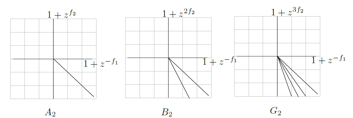
Figure 1: ${\mathcal{A}}$-scattering diagrams for rank 2 finite type.

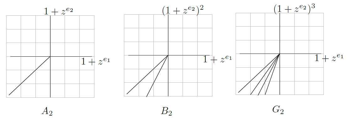
Figure 2: ${\mathcal{X}}$-scattering diagrams for rank 2 finite type.

Mutation of scattering diagrams

As noted in the previous section, a seed determines canonically a scattering diagram. Two mutation-equivalent seeds would then give two different scattering diagrams. It is natural to consider ‘mutation equivalent’ scattering diagrams. This equivalence is given by piecewise linear maps on the lattices which are very similar to those in Section 3 and hence we will state here.

Consider two seeds s and $\textbf{s}^{\prime}$ which are just one mutation step apart, i.e. $\textbf{s}^{\prime}=\mu_{k}(\textbf{s})$ for some $k\in I$. Then the corresponding scattering diagrams $\mathfrak{D}_{\textbf{s}}$ and $\mathfrak{D}_{\textbf{s}^{\prime}}$ are equivalent to each other by the transformation $T_{k}:M^{\circ}\rightarrow M^{\circ}$,

$$T_{k}(m)=\left\{\begin{array}[]{l r}m+\langle d_{k}e_{k},m\rangle v_{k},&\text{ for }m\in\mathcal{H}_{k,+}\\ m,&\text{ for }m\in\mathcal{H}_{k,-}\end{array}\right.$$ (1)

for $m\in M^{\circ}$, $v_{k}=p^{*}(e_{k})$, and $\mathcal{H}_{k,+}=\{m\in M_{\mathbb{R}}|\langle e_{k},m\rangle\geq 0\}$, $\mathcal{H}_{k,-}=\{m\in M_{\mathbb{R}}|\langle e_{k},m\rangle\leq 0\}$. Extending $T_{k}$ to the wall functions (ghkk, , Theorem 1.24) will lead us to another consistent scattering diagram $T_{k}(\mathfrak{D}_{s})$ which is shown to be equivalent to $\mathfrak{D}_{\mu_{k}(s)}$.

We can similarly define the mutation for the ${\mathcal{X}}$ scattering diagrams from ${\mathcal{A}}_{\text{prin}}$. For the scattering diagram of type $A_{2}$ in Figure 2, we can obtain the mutation process for the ${\mathcal{X}}$ scattering diagram as in Figure 3 and Figure 4.

Figure 3: Mutation of the ${\mathcal{X}}$ scattering diagram of type $A_{2}$ starting at the index $1$

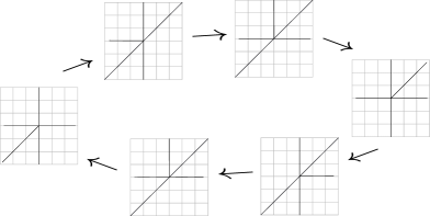
Figure 4: Mutation of the ${\mathcal{X}}$ scattering diagram of type $A_{2}$ starting at the index $2$

Note that the scattering diagrams are determined by seeds while the mutation of seeds are given by blow ups and blow downs of toric varieties. Thus the mutation of scattering diagrams actually represents this procedure of blowups and blowdowns. We are going to discuss a similar construction in Section 3 with a symplectic perspective.

Theta functions and the canonical algebras

Theta functions give the generators of the canonical basis of the cluster algebras. Given the cluster variety $V={\mathcal{A}},{\mathcal{A}}_{\text{prin}},{\mathcal{X}}$, the corresponding character lattice is $L=M^{\circ}$, $\widetilde{M}^{\circ}$, or $N$. A theta function $\vartheta_{p}$ is associated to each point $p\in L$ by a combinatorial object – broken lines which are piecewise linear paths in $L_{\mathbb{R}}$ together with decorating monomials at each linear segment.

The free module generated by theta functions is endowed with an algebra structure from the multiplication between theta functions. Indeed the structure constants in the multiplications of theta functions can be given in terms of counting broken lines. The product of two theta functions can be expressed as

$$\vartheta_{p}\cdot\vartheta_{q}=\sum_{r}\alpha(p,q,r)\vartheta_{r},$$ (2)

where the structure constants $\alpha\left(p,q,r\right)$ can be explicitly defined by counting broken lines with certain boundary conditions (ghkk, , Proposition 6.4). In this finite type case, the structure constants $\alpha$ define ((ghkk, , Corollary 8.18)) the finitely generated $\mathbb{C}$-algebra structure on

$$\operatorname{can}(V):=\bigoplus_{r\in L}\mathbb{C}\cdot\vartheta_{r}.$$

We will then define $X:=\operatorname{Spec}(\operatorname{can}(V))$.

2.2 Positive polytopes

With the multiplication structure of the theta functions, we can now state the definition of a positive set– the property required for a set and its dilations to define a graded ring.

For $S\subseteq L_{\mathbb{R}}=L\otimes\mathbb{R}$ a closed subset, define the cone of $S$ as

$$\textbf{C}(S)=\overline{\{(p,r)\mid p\in rS,r\in\mathbb{R}_{\geq 0}\}}\subset L_{\mathbb{R}}\times\mathbb{R}_{\geq 0}.$$

Denote $dS(\mathbb{Z})=\mathbf{C}(S)\cap\left(L\times\{d\}\right)$ which is viewed as a subset of $L$.

A closed subset $S\subset L_{\mathbb{R}}$ is called positive if for any non-negative integers $d_{1}$, $d_{2}$, any $p_{1}\in d_{1}S(\mathbb{Z})$, $p_{2}\in d_{2}S(\mathbb{Z})$, and any $r\in L$ with $\alpha(p_{1},p_{2},r)\neq 0$, then $r\in(d_{1}+d_{2})S(\mathbb{Z})$.

In the ongoing example of cluster varieties of type $A_{2}$, we consider the polytope with vertices $(1,0),(0,1),(-1,0),(0,-1),(1,-1)$ as indicated in Figure 5. Note that this polytope is in the ${\mathcal{X}}$ diagram thus there is a flip from Figure 21. This polytope is indeed positive. In Section 3.1, there is a detail discussion of such a polytope in the ${\mathcal{A}}$ side. A similar calculation in this ${\mathcal{X}}$ case will still hold, thus this will correspond to the del Pezzo surface of degree 5 ghkk .

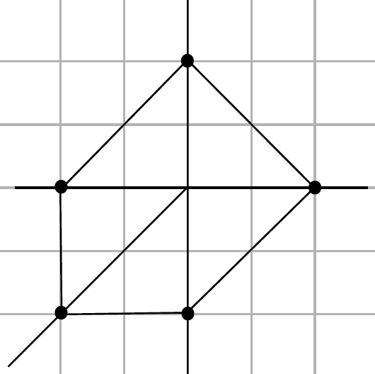
Figure 5: Positive polytope of ${\mathcal{X}}$ cluster variety of type $A_{2}$.

We can apply the mutation sequences in Figure 3 and 4 to the polytope in Figure 5. Mutations of the polytopes as in Figure 6 and 7 will be obtained respectively.

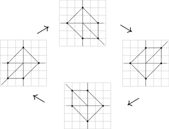
Figure 6: Mutation of polytope starting from index $1$

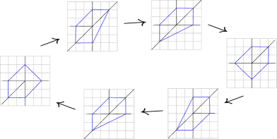
Figure 7: Mutation of polytope starting from index $2$

In the next section, we will describe mutations of the polytopes from a symplectic point of view. We observe that the mutation sequences of polytope in Figure 6 and 7 are the same as the sequences in Figure 23 and 24 respectively. The cluster mutation of the scattering diagrams comes from a change of seed data, i.e. a change of the initial variables. Thus the underlying spaces are all isomorphic.

Compactifications from positive polytopes

We will roughly go over the geometric meaning behind the positive polytopes in this section. The motivation can be seen as the construction of projective toric varieties from the convex polytopes.

For rank 2 cluster varieties, since the ${\mathcal{A}}$ scattering diagrams are well defined, we can consider $\bar{S}$ the positive polytopes in the ${\mathcal{A}}$ scattering diagrams. For this set $\bar{S}$, define $\widetilde{S}=\bar{S}+N_{\mathbb{R}}$ which is obviously positive. Thus we can define the graded ring

$$\widetilde{R}_{\widetilde{S}}=\bigoplus_{d\geq 0}\bigoplus_{q\in d\widetilde{S}(\mathbb{Z})}\mathbb{C}\vartheta_{q}x^{d}\subset\operatorname{can}({\mathcal{A}}_{\text{prin}})[x],$$

with grading defined by $x$.

Define $Y_{{\mathcal{A}}_{\text{prin}}}:=\mathrm{Proj}(\widetilde{R}_{S})\rightarrow T_{M}$. For the ${\mathcal{A}}$ variety, we take $Y_{{\mathcal{A}}}$ as the fiber over $e\in T_{M}$ in this map. More generally, for the ${\mathcal{A}}_{t}$ variety, $t\in T_{M}$, we can still take $Y_{{\mathcal{A}}_{t}}$ as the fiber over $t\in T_{M}$. Consider $X=\operatorname{Spec}(\operatorname{can}(V))$, for $V={\mathcal{A}}_{\text{prin}},{\mathcal{A}}_{t}$, as in the previous subsection. Define $B=Y\setminus X$. Then ghkk showed that, $X$ is a Gorenstein scheme with trivial dualizing sheaf, in particular, for $V={\mathcal{A}}_{\text{prin}},{\mathcal{A}}_{t}$, $X$ is a $K$-trivial Gorenstein log canonical variety. In this finite rank 2 case, for $V={\mathcal{A}}_{\text{prin}},{\mathcal{A}}$, $X\subseteq Y$ is a minimal model, i.e. $Y$ is a projective normal variety, $B\subset Y$ is a reduced Weil divisor, $K_{Y}+B$ is trivial, and $(Y,B)$ is log canonical.

For the case of the ${\mathcal{X}}$ varieties, as indicated in Section 2.1, the ${\mathcal{X}}$ varieties are quotients of the ${\mathcal{A}}_{\text{prin}}$ varieties. Thus we will consider still consider ${\mathcal{A}}_{\text{prin}}$ but instead see the lattice as $\widetilde{M}^{\circ}$ instead of $\widetilde{N}$ (which are actually isomorphic). We can repeat the same procedure as before and then obtain the compactification of $X=\operatorname{Spec}(\operatorname{can}({\mathcal{X}}))$. The scheme $X$ is also a $K$-trivial Gorenstein log canonical variety.

2.3 Canonical scattering diagrams

In the last section, we note that the cluster mutations of the scattering diagrams are not changing the underlying schemes. We are proposing another type of mutation which is given by the monodromy on $B$. We are going to understand the ideas behind from the mirror construction suggested by Gross, Hacking, and Keel in GHKlog . In Section 3.1, we will discuss the affine structure and monodromy from the SYZ perspective.

Consider a pair $(Y,D)$, where $Y$ is a smooth rational projective surface, and $D$ is an anti-canonical cycle of projective lines. We will call such a pair a Looijenga pair. Let $X=Y\setminus D$. The tropicalization of $(Y,D)$ is a pair $(B,\Sigma)$, where $B$ is an integral linear manifold with singularities, and $\Sigma$ is a decomposition of $B$ into cones. The pair $(B,\Sigma)$ can be constructed by associating each node $p_{i,i+1}$ of $D$ a rank two lattice with basis $v_{i}$, $v_{i+1}$. Denote the cone generated by $v_{i}$, $v_{i+1}$ as $\sigma_{i,i+1}\subset M_{i,i+1}\otimes\mathbb{R}$. The cones $\sigma_{i,i+1}$ and $\sigma_{i-1,i}$ are glued over the ray $\rho_{i}=\mathbb{R}_{\geq 0}v_{i}$ to obtain a piecewise linear manifold $B$ homeomorphic to $\mathbb{R}^{2}$ and $\Sigma=\{\sigma_{i,i+1}\}\cup\{\rho_{i}\}\cup\{0\}$.

The integral affine structure on $B_{0}=B\setminus\{0\}$ can be defined by the charts

$$\psi_{i}:U_{i}=\mbox{Int}(\sigma_{i-1,i}\cup\sigma_{i,i+1})\rightarrow M_{\mathbb{R}},$$

where

$$\psi_{i}(v_{i-1})=(1,0),\ \psi_{i}(v_{i})=(0,1),\ \hbox{and}\quad\psi_{i}(v_{i+1})=(-1,-D^{2}),$$

and $\psi_{i}$ is linear on $\sigma_{i-1,i}$ and $\sigma_{i,i+1}$.

Now consider $Y$ the del Pezzo surface of degree 5 and $D$ the anti-canonical cycle of five (-1)-curves. The construction of the charts $\psi$ will then give

$$\psi(v_{1})=(1,0),\psi(v_{2})=(0,1),\psi(v_{3})=(-1,1),\psi(v_{4})=(-1,0),\psi(v_{5})=(0,-1).$$

Note however that having $\psi(v_{4})=(-1,0),\psi(v_{5})=(0,-1)$ will lead to

$$\psi(v_{1})\leadsto(1,-1),\ \psi(v_{2})\leadsto(1,0)$$

and this is NOT what we began with: $\psi(v_{1})=(1,0)$, and $\psi(v_{2})=(0,1)$. Thus we would like to identify the cone spanned by $(1,0)$ and $(0,1)$, and the cone spanned by $(-1,1)$ and $(1,0)$. This introduces the monodromy

$$(1,0)\mapsto(1,1),\quad(0,1)\mapsto(1,0),$$

to $B_{0}$. The affine structure is illustrated in Figure 8.

Figure 8: The tropicalization $(B,\Sigma)$ of the del Pezzo surface of degree 5

Now we would like to define the canonical scattering diagrams from $(B,\Sigma)$. Rather than obtaining the diagrams by the algorithmic process with some initial data in GS KS , the canonical scattering diagrams are defined via some Gromov-Witten type invariants. We will discuss the two types of diagrams are the ‘same’ later in the discussion about how to go from canonical scattering diagrams to cluster scattering diagrams. A wall ghks_cubic in $B$ is a pair $(\mathfrak{d},f_{\mathfrak{d}})$ where $\mathfrak{d}\subset\sigma_{i,i+1}$, for some $i$, is a ray generated by $av_{i}+bv_{i+1}\neq 0$, $a,b\in\mathbb{Z}$ relatively prime, and $f_{\mathfrak{d}}=1+\sum_{k\geq 1}c_{k}X_{i}^{-ak}X_{i+1}^{-bk}\in\mathbb{C}[[X_{i}^{-a}X_{i+1}^{-b}]]$ with some finiteness properties, and where $c_{k}$ corresponds to the curve counting invariants. Note that the description of the wall functions $f_{\mathfrak{d}}$ indicates that all the wall are outgoing in the sense stated in the last section. Then the scattering diagrams are again the collections of walls. For example, the canonical scattering diagram associated to Figure 8 is shown in Figure 9.

Figure 9: Canonical scattering diagram

Let $B(\mathbb{Z})$ be the set of points of $B_{0}$ with integral coordinates in an integral affine chart and $\{0\}$. Theta functions $\vartheta_{q}$, $q\in B(\mathbb{Z})$, can similarly be defined on the scattering diagrams. The set of theta functions again generates an algebra structure GHKlog in terms of broken lines. In the finite case, we can simply consider $A=\oplus_{q\in B(\mathbb{Z})}\vartheta_{q}$.

Analogous to the setting in the cluster scattering diagrams, we can use the Rees construction to compactify the mirrors gross2019intrinsic . Positive polytopes with respect to the affine structures can be similarly defined to give a graded algebra. Using mandel2016tropical or the argument in cpt , the polytopes are broken line convex. In this case, since all the walls are outgoing, the positive polytopes are simply convex with respect to the affine structures.

Relation to the cluster scattering diagrams

In the case of $Y$ a non-singular toric surface and $D=\partial Y$ the toric boundary of $D$, the affine structure on $B$ extends across the origin. This identifies $(B,\Sigma)$ with $M_{\mathbb{R}},\Sigma_{Y}$, where $\Sigma_{Y}$ is a fan for $Y$.

Now given a Looijenga pair. Assume there is a toric model $p:(Y,D)\rightarrow(\bar{Y},\bar{D})$ which blows up distinct points $x_{ij}$ on $D_{i}$. A toric model of $(Y,D)$ is a birational morphism $(Y,D)\rightarrow(\bar{Y},\bar{D})$ to a smooth toric surface $\bar{Y}$ with its toric boundary $\bar{D}$ such that $D\rightarrow\bar{D}$ is an isomorphism. Consider the tropicalisation $(\bar{B},\bar{\Sigma})$ of $(\bar{Y},\bar{D})$. Thus $\bar{B}\cong M_{\mathbb{R}}=\mathbb{R}^{2}$ and $\bar{\Sigma}$ is the fan for $\bar{Y}$. Then there is a canonical piecewise linear map

$$\nu:B\rightarrow\bar{B}$$

which restricts to an integral affine isomorphism on the maximal cones in $\sigma$ and $\bar{\Sigma}$. One can then define the scattering diagram $\mathfrak{D}$ as outlined in Section 2.1 or as in (GHKlog, , Definition 3.21) for the more general setting. This step can be seen as ‘pushing the singularities to infinity’ or ‘moving worms’ KS . By definition, the singularity of the affine structure is at $\{0\}$ as indicated in Figure 8. Then the singularity can be imagined to be pushed to the infinity of the two incoming walls. The map $\nu$ can be extended to act on the canonical scattering diagram $\mathfrak{D}^{\text{can}}$. It is shown that GHKlog $\bar{\mathfrak{D}}=\nu(\mathfrak{D}^{\text{can}})$.

We have discussed in Section 2.1 that every cluster variety can be described as blow ups of a toric variety, which give the toric models for the cluster variety. Thus the cluster scattering diagrams can be seen as the diagrams arising from the canonical scattering diagrams by the map $\nu$ (as pushing singularities to infinity).

Mutation of polytopes according to the affine structures

One can imagine or with symplectic motivation as in Section 3.1, the ‘pushing singularities to infinities’ procedure is more general than just having singularities at the origin. For example, we can consider Figure 10 which we only push one of the singularities to infinity, resulting in a scattering diagram with one incoming wall.

Figure 10: Scattering diagrams with monodromy.

The monodromy in Figure 10 is $\begin{pmatrix}1&0\\ 1&1\end{pmatrix}$, or $(1,0)\mapsto(1,1)$, $(0,1)\mapsto(0,1)$. The polytope in Figure 5 with respect to this affine structure would then be of the form in Figure 11.

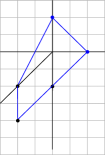
Figure 11: Positive polytope with respect with the underlying affine structure

We can apply the sequence of mutations in Figure 3 to the polytope in Figure 11 and then obtain a new sequence of mutation polytopes (Figure 12). Putting the polytope in Figure 5 into the sequence (Figure 12) will get us the sequence Figure 26 which is motivated from the symplectic perspective.

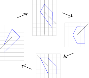
Figure 12: Mutation of polytopes with monodromy

The singularities can also be located on the walls instead of just at infinity or the origin. For example, one can obtain the canonical scattering diagram shown in Figure 13. Similar calculation shown in dp5 indicates that the scattering diagram is consistent.

Figure 13: Scattering diagram with monodromy on the walls.

Note that the portions of the walls which go from the singularities to infinity are all outgoing. Thus using the idea in (cpt, , Remark 6.2), we can consider convex sets in this affine structure. For example, one can construct the polytope as in Figure 14.

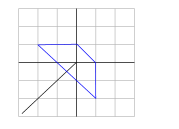
Figure 14: Polytope lives in the affine structure indicated in Figure 13.

Applying the mutation sequence as in Figure 3, we obtain the sequence of polytopes described in Figure 15. Interestingly, this is the same sequence as in Figure 27 which is motivated from the symplectic perspective.

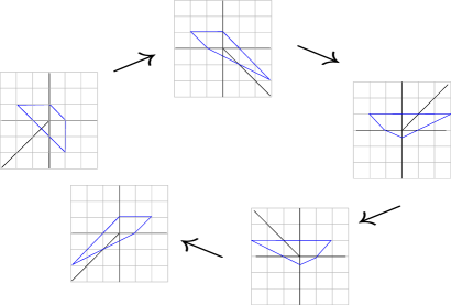
Figure 15: Mutation for the polytope in Figure 14

2.4 Type $B_{2}$ and $G_{2}$

The other types are similar and thus we only roughly go over the mutations of type $B_{2}$ and $G_{2}$. For type $B_{2}$, we will take the same skew-symmetric form with $d_{1}=1$, and $d_{2}=2$ as our fixed data. We can again take the initial seed as $\textbf{s}=\{(1,0),(0,1)\}$. Then we will obtain the ${\mathcal{A}}$ and ${\mathcal{X}}$ scattering diagrams as in Figure 1 and 2. If we mutate at index $1$ first, we can get the mutation of scattering diagrams very similar to the type $A_{2}$ case.

For type $B_{2}$, we can again take the primitive generators of the walls and then consider the polytope as the convex hull of those vertices. By using cpt , this polytope is a positive polytope. The multiplication of the theta functions tells us bat_finitetype that the corresponding space is the del Pezzo surfaces of degree 6. The mutation sequence of the polytopes is described in Figure 16.

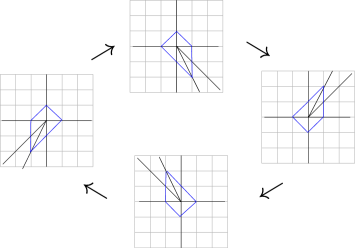
Figure 16: Mutation of polytope for type $B_{2}$

One may want to repeat the same trick on the type $G_{2}$. The sad fact is that the if we are taking the convex hull of the primitive generators of the walls, the resulting polytope would no longer be positive. This is because the polytope is no longer broken line convex as indicated in cpt . Since we only care about the incoming walls for broken line convexity cpt , one can see that the top left polytope in Figure 29 in the next section is broken line convex. The mutation sequence of the $G_{2}$ scattering diagrams are similar to those for type $A_{2}$ and $B_{2}$. Without duplicating, one can see that the mutation indicate in Figure 29 is in fact the cluster mutation of scattering diagrams. Thus the mutation of polytopes follows correspondingly. This again tells us that the mutation sequences of the polytope with the algebro-geometric and symplectic viewpoints coincide.

3 Mutations in symplectic geometry

We begin this section giving a perspective on understanding cluster varieties, as well as scattering diagrams, as a way of building mirrors under SYZ SYZ96 $T$-duality. In particular, we explain how scattering diagrams can be related to almost toric fibrations. Later, we explain how one can see compactifications of $2$-dimensional cluster varieties into del Pezzo surfaces from an almost toric fibration perspective.

3.1 Cluster varieties and Mirror Symmetry

In this section we will sketch how to relate a scattering diagram data (described in Section 2), for constructing a log-CY variety $X$, with the base of an almost-toric fibration (ATF), describing a SYZ SYZ96 singular Lagrangian fibration of $(X,\omega)$, with respect to a Kähler form $\omega$ in $X$.

Almost Toric Fibrations

Informally speaking an almost toric fibrations (ATF) in a symplectic 4-manifold $X$ is a smooth map to a two dimensional base $B$, whose regular fibres are Lagrangian tori, whose allowed singular fibres are of three kinds:

• point (toric - rank 0 elliptic) – locally equivalent to the moment map at the origin in $\mathbb{C}^{2}$ with the standard toric action, $(e^{i\theta_{1}},e^{i\theta_{2}})\cdot(x,y)=(e^{i\theta_{1}}x,e^{i\theta_{2}}y)$;

• circle (toric - rank 1 elliptic) – locally equivalent to $S^{1}\times\{0\}\subset\mathbb{C}^{*}\times\mathbb{C}$ with the standard toric action;

• nodal (a pinched torus) – with some local model described for the singular point. [See Sy03 ; SyLe10 for precise definition, and see Section 3.1 for a local model of the nodal fibre.]

The toric singularities appear on the boundary of the base, while the nodal singularities project into the interior. For a precise definition of ATFs see Sy03 .

Away from the singular fibres, by the Arnold-Liouville theorem Ar_book , $X$ admits locally action angle coordinates $(p_{1},p_{2},\theta_{1},\theta_{2})$ and the fibration is locally equivalent to $(p_{1},p_{2},\theta_{1},\theta_{2})\mapsto(p_{1},p_{2})$, in other words, away from singular fibres $X$ equivalent to $T^{*}B/\Lambda^{*}$, for some lattice $\Lambda^{*}$. Hence, $B$ carries a natural dual lattice $\Lambda\subset TB$. The lattice has monodromy as we go around the nodal fibre, which is a shear in the direction dual to the collapsing cycle of that nodal fibre. Locally, the coordinates $(p_{1},p_{2})$, can be thought as the flux $\mathfrak{f}\in H^{1}(T^{2},\mathbb{R})$ relative to the Lagrangian fibre associated with $(0,0)$. The flux $\mathfrak{f}(\gamma)$ measures the symplectic area of a cylinder swept by a cycle $\gamma\in H_{1}(T^{2},\mathbb{Z})$ as we move in a path of Lagrangian fibres connecting $(0,0)$ to $(p_{1},p_{2})$. [See, for instance, ShToVi18 for a more complete understanding of flux in ATFs.]

So, in practice, we visualise the base minus a set of cuts (one for each nodal fibre) affinely embedded into $\mathbb{R}^{2}$ endowed with the standard affine structure. We call them almost-toric base diagrams (ATBDs) representing the ATF. The same ATF can be represented by different ATBDs, by changing the set of cuts.

Figure 17 shows the base diagram of 3 different ATFs in $\mathbb{C}^{2}$; the right-most diagrams on Figure 18 are different diagrams representing the same ATF in $\mathbb{C}^{2}\setminus\{xy=1\}$, related by a change of cut; Figures 23–33 contain examples of ATBDs in closed 4 manifolds. In these diagrams, the crosses represent the nodal fibres, the dashed lines the cuts, the edges the rank 1 and the dots rank 0 toric singularities.

Remark 1

We expect the above mentioned ATFs to be realisable as a special Lagrangian fibration in the complement of a complex divisor projecting to the boundary of the ATF, with respect to a holomorphic volume form with poles on these divisor. This is true for the fibration presented in Section 3.1, but we will avoid talking about the ”special” condition.

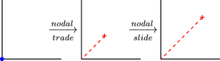
Figure 17: Nodal trade and nodal slide operations in ATFs.

There are two ways of modifying ATFs within the same symplectic manifold $X$, known as nodal trade and nodal slide Sy03 . The diagrams in Figure 17 illustrate the change of the ATBDs after a nodal trade and a nodal slide. In del Pezzo surfaces, the monotone symplectic 4-manifolds, we defined mutation of an ATBD, the process of sliding one nodal fiber through the monotone fibre, and then redrawing the diagram by changing the direction of the cut used to slide Vi14 ; Vi16a . In the end, the ATBD mutates by slicing it in the direction of the cut and applying the inverse of the corresponding monodromy, which is a shear in the primitive direction associated to the cut. This transformation is the same polytope mutation as in ACGK12 ; AkKa16 , and completely analogous to the mutation of seeds, and scattering diagram we will discuss later. We can extend this notion of symplectic mutation to exact almost toric manifold, for instance, the complement of an anti-canonical divisor in a del Pezzo. In this case, the mutation corresponds to sliding a nodal fibre through the exact torus and then transferring the associated cut to the opposite side.

Local model for nodal fibre and wall-crossing

We briefly recall ATF presented in (Au07, , Section 5), (Au09, , Section 3.1.1). This ATF appeared before in ElPo93 and also in (Gro97, , Example 1.2), where it was shown to be a special Lagrangian fibration [with respect to certain holomorphic volume form]. We consider $X^{\vee}=\mathbb{C}^{2}\setminus\{xy=1\}$, with $\omega^{\vee}=\frac{i}{2}\left(dx\wedge d\bar{x}+dy\wedge d\bar{y}\right)$ the standard symplectic form. Using $f:X^{\vee}\to\mathbb{C}\setminus\{1\}$, $f(x,y)=xy$, Auroux builds an ATF by parallel transport of orbits of the $S^{1}$ action $e^{i\theta}\cdot(x,y)=(e^{i\theta}x,e^{-i\theta}y)$, over circles in the base of $f$ centred at $1$. One then gets Lagrangian torus fibres, parametrised by $(r,\lambda)\in\mathbb{R}_{>0}\times\mathbb{R}$, as:

$$T_{r,\lambda}=\{(x,y)\in\mathbb{C}^{2};r=|xy-1|,\lambda=|x|^{2}-|y|^{2}\}.$$

Note that there is a nodal fibre $T_{1,0}$, that contains $(0,0)$, the fixed point of the $S^{1}$ action.

This almost toric fibration can be represented by applying a nodal trade to the standard toric fibration of $\mathbb{C}^{2}$, replacing the boundary divisor $\{xy=0\}$ with the smooth divisor $\{xy=1\}$, and then deleting this divisor living over the boundary of the base, as illustrated by Figure 18. Indeed, replacing the role of $1$ by $0$ in the above fibration, i.e., considering parallel transport over circles concentric at $0$ (considering $r=|xy|$) one obtain precisely the standard toric fibration of $\mathbb{C}^{2}$. So, considering analogous fibrations by changing $0$ to $1$ in the definition of $r$ constitutes a nodal trade, and moreover, varying the value of $c\in\mathbb{R}_{>0}$ in the definition of $r=|xy-c|$ provides different fibrations related by nodal slides.

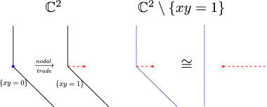
Figure 18: Nodal trade and an ATF for the complement of a conic. The left diagrams are a shear by $(0,-1)$ of the diagrams in Figure 17. The rightmost diagrams, represent the same ATF, and differ by changing the direction of the cut.

Wall-crossing

Dualising this torus fibration, one gets the mirror variety $X_{\Lambda}$ of $X^{\vee}$, over the Novikov field $\Lambda=\{\sum_{i=0}^{n}a_{i}T^{\sigma_{i}};a_{i}\in\mathbb{C},\sigma_{i}\in\mathbb{R},\lim_{i}\sigma_{i}=\infty\}$, which is the moduli of almost-toric fibres (special Lagrangians), endowed with unitary $\Lambda^{*}$-local systems. We will be able to relate the valuation $\mathrm{val}(u)=\min\{\sigma_{i};a_{i}\neq 0\}$ of an element $u\in\Lambda$ with the above mentioned flux, whenever $\mathrm{val}(u)$ measures the symplectic area of a disk with boundary in a varying family of the Lagrangian torus fibres. [Notation: $\Lambda_{0}=\{u\in\Lambda;\mathrm{val}(u)\geq 0\}$, $\Lambda_{+}=\{u\in\Lambda;\mathrm{val}(u)>0\}$, $\Lambda^{*}=\{a_{0}+\Lambda_{+};a_{0}\in\mathbb{C}^{*}\}$.] We will later consider the mirror of $X^{\vee}$ as $X=X_{\mathbb{C}}$ over $\mathbb{C}$, by replacing $T$ with $e^{-1}$.

So we replace the Lagrangian fibre $T^{2}$, by the dual $\Lambda$-torus of unitary local systems $\hom(\pi_{1}(T^{2});\Lambda^{*})\cong(\Lambda^{*})^{2}$. Locally identifying each relative class, $\beta\in\pi_{2}(\mathbb{C},T_{r,\lambda})$, Auroux defined a function $z_{\beta}:X_{\Lambda}\to\Lambda$, for a local system $\nabla$ in $T_{r,\lambda}$, $z_{\beta}(\nabla)=T^{\omega^{\vee}(\beta)}\nabla\cdot\partial\beta$. Choosing a basis $\{\alpha,\beta\}$ of $\pi_{2}(\mathbb{C},T_{r,\lambda})$, one gets that $w:=z_{\alpha},\ u:=z_{\beta}$, define local coordinates of $X_{\Lambda}$. After that, the idea is to define a superpotential function $W:X_{\Lambda}\to\Lambda_{+}$, which is locally defined as $W(u,w)$, and whose monomials encode the relative Gromov-Witten count of Maslov index 2 holomorphic disks in $\mathbb{C}$ with boundary on the torus fibre endowed with the respective local system determined by $(u,w)$. [The pair $(X_{\Lambda},W)$ is called the Landau-Ginzburg model that is mirror dual to $\mathbb{C}$ with respect to the divisor $D=\{xy-1\}$. We refer the reader to Au07 ; Au09 for details on mirror symmetry in the complement of divisors.]

The issue is that, in the naive definition of the mirror, the superpotential $W$ is discontinuous. This is due to the presence of fibres $T_{1,\lambda}$, $\lambda\neq 0$, which bounds Maslov index $0$ holomorphic disks. Let’s denote the relative class represented by this Maslov 0 disks by $\alpha$ for $\lambda<0$, and $-\alpha$ for $\lambda>0$. In (Au09, , Section 3.1.1), it is shown that for $r<1$, the fibres $T_{r,\lambda}$ (called Chekanov type) bound one holomorphic disk, in a class we name $\beta$. So $W(u,w)=u$, for these fibres. The fibres $T_{r,\lambda}$, for $r>1$, (called Clifford type) bound 2 holomorphic disks in relative classes $\beta_{1}$, $\beta_{2}$, and hence the superpotential is of the form $W(z_{1},z_{2})=z_{1}+z_{2}$, where $z_{i}=z_{\beta_{i}}$.

We see in (Au09, , Section 3.1.1) that as $r$ approaches $1$, from $r>1$, we get $\alpha=\beta_{1}-\beta_{2}$ (hence $w=z_{1}z_{2}^{-1}$). Moreover, if we cross the wall at $\lambda<0$, the class $\beta$ is naturally identified with $\beta_{2}$, and if we cross the wall at $\lambda>0$, the class $\beta$ is naturally identified with $\beta_{1}=\beta_{2}+\alpha$ [which is not so surprising, as the monodromy around the nodal fibre in the ATF would fix $\partial\alpha$ and maps $\partial\beta\to\partial\beta+\partial\alpha$]. So the superpotential $W$ should be corrected by the term $(1+w^{\pm 1})$, representing the fact that the holomorphic disk on class $\beta$, would not only survive past the wall, but the superpotential would also acquire a holomorphic disk in class $\beta\pm\alpha$, coming from the gluing of the Maslov 2 holomorphic disk on class $\beta$ with the Maslov 0 holomorphic disk on class $\pm\alpha$. Then, instead of $u$ becoming $z_{2}$ as we cross over $\lambda>0$, we should correct it to become $u=z_{2}(1+w)=z_{2}+z_{1}$, and instead of $u$ becoming $z_{1}$ as we cross over $\lambda<0$, we should correct it to become $u=z_{1}(1+w^{-1})=z_{1}+z_{2}$, and, thus, ensuring the continuity of $W$.

By naming $v=z_{2}^{-1}$, so $z_{1}=v^{-1}w$, we get the corrected $u=v^{-1}(1+w)=v^{-1}w(1+w^{-1})$. We see that the corrected (and completed) mirror $X_{\Lambda}$, is given by

$$X_{\Lambda}=\{(u,v,w)\in\Lambda^{2}\times(\Lambda\setminus\{0\});uv=1+w\}.$$

Figure 19 below describes the mirror SYZ fibrations on $X^{\vee}$ and $X_{\Lambda}$. We list several remarks about the diagrams in Figure 19 and the mirror $X_{\Lambda}$.

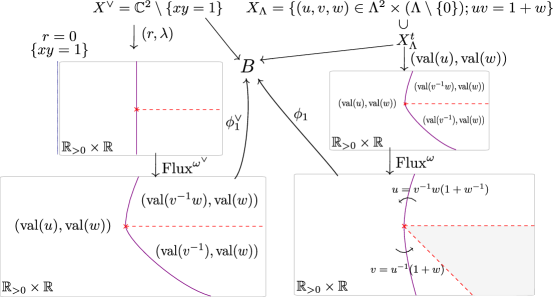
Figure 19: SYZ fibrations for the complement of a conic, which is self-mirror, when considering $X_{\mathbb{C}}$.

Remark 2

We see that $X_{\Lambda}$ is given by gluing two torus charts $(u,w)\in(\Lambda\setminus\{0\})^{2}$, and $(v,w)\in(\Lambda\setminus\{0\})^{2}$, by a rational map defined in the complement of $\{w=-1\}$. So, for instance, the case $u=0$ would be realised as $(v,-1)$ in the $(v,w)$-chart.

Remark 3

Considering the symplectic form $\omega^{\vee}$ in $X^{\vee}$, the Lagrangian torus fibration would be viewed in a truncated part of the $(u,w)$-chart, with $0<\mathrm{val}(u)\leq a(\mathrm{val}(w))$ or in the $(v,w)$-chart, with $a(\mathrm{val}(w))\leq\mathrm{val}(v^{-1})<\infty$ for $\mathrm{val}(w)<0$, for instance. These bounds on the valuation would give us $X_{\Lambda}^{t}$, a truncated version of the mirror $X_{\Lambda}$. But in symplectic geometry, we can add to $(X^{\vee},\omega^{\vee})$ a contact boundary $\partial X^{\vee}$, and it is most natural to consider a completion procedure called the symplectization of $X^{\vee}$ with respect to this boundary. This endows $X^{\vee}$ with a different symplectic form $\omega^{\vee}_{S}$. It is equivalent to consider an infinite inflation of $(\mathbb{C}^{2},\omega^{\vee})$ with respect to the divisor $D=\{xy=1\}$. In this limit we would have $\mathrm{val}(u)\to\infty$, and we would get the completed mirror $X_{\Lambda}$.

Remark 4

The expectation regarding the correspondence between the count of Maslov index 2 disks with boundary on a SYZ fibre and its tropical counterpart was proven in lin2020enumerative for a SYZ fibration on the complement of an smooth anti-canonical divisor in a del Pezzo surface. More precisely, given a del Pezzo surface $Y$ and a smooth anti-canonical divisor $D$, there exists a special Lagrangian fibration on $Y\setminus D$ with respect to the complete Ricci-flat Tian-Yau metric CJL . To understand the Landau-Ginzburg superpotential of $Y$, there exists a sequence of Kähler forms $\omega_{i}$ on $Y$ converging to the Tian-Yau metric pointwisely with $\int_{Y}\omega_{i}^{2}\rightarrow\infty$ (lin2020enumerative, , Lemma 2.4). Thus, these superpotentials of the special Lagrangian fibres can be defined with respect to $\omega_{i}$, $i\gg 0$ and the superpotentials coincide with the tropical counterpart (lin2020enumerative, , Theorem 5.19). This gives a geometric explanation of the renormalization procedure of taking valuation going to infinity.

Remark 5

In the $(r,\lambda)$ projection of Figure 19, the singular fibre in position $(1,0)$ is depicted by an $\times$, and the wall of fibres with $r=1$ that bound Maslov index 0 disks are represented by a line. This $(r,\lambda)$ coordinate does not respect the natural affine structure on the complement of the singular fibre of $B$. We instead consider $\mathrm{Flux}^{\omega^{\vee}}$, the flux with respect to a limiting fibre lying over $(0,0)$, in the next diagram. This map is then continuous, but not differentiable over the dashed ray $r\geq 1$, $\lambda=0$, which we call the cut. Moreover, this composition represents the map to the base diagram depicted in the rightmost picture of Figure 18. The map $\phi_{1}^{\vee}$ is then an affine isomorphism to $B$ minus the cut. The affine structure of $B$ minus the node, is described by the gluing of the chart $\phi_{1}^{\vee}$ and a chart $\phi_{2}^{\vee}$, going from the third diagram of Figure 18, corresponding to taking the cut associated to $0<r\leq 1$, $\lambda=0$. The symplectic manifold $X^{\vee}$ can be thought then as a local model for gluing in the nodal fibre to the manifold constructed from gluing the Lagrangian torus fibres associated to $\phi_{1}^{\vee}$ and $\phi_{2}^{\vee}$. This is essentially the same model as the description of $X^{\vee}$ as a self-plumbing of $T^{*}S^{2}$ given in (Sy03, , Section 4.2).

Remark 6

The affine structure on $B$ for the dual mirror fibration $X_{\Lambda}\to B$ is endowed with the dual affine structure in the complement of the node. We call the map that adjusts this affine structure in $\mathbb{R}^{2}$, $\mathrm{Flux}^{\omega}$. In the case we take the SYZ mirror $X_{\mathbb{C}}$ over $\mathbb{C}$ (by replacing $T$ by $e^{-1}$), it endows a symplectic form $\omega$ as described in (Au09, , Proposition 2.3). In this case, $\mathrm{Flux}^{\omega}$ becomes the actual flux with respect to this symplectic form.

Remark 7

The monodromy around the singular fibre of $X^{\vee}\to B$, represented by the bottom left diagram of Figure 19, is given by $M^{\pm 1}$, for $M=\begin{bmatrix}1&-1\\ 0&1\end{bmatrix}$, fixing the cut $(1,0)$. Then, the monodromy around the node for the rightmost diagram representing $X_{\Lambda}\to B$ is given by $(M^{T})^{\mp 1}$, with $(M^{T})^{-1}=\begin{bmatrix}1&0\\ 1&1\end{bmatrix}$. We see that this fixes the coordinate $w$, associated to $(0,1)$, which we then name $\vartheta_{(0,1)}$, and it sends the coordinate $v^{-1}=\vartheta_{(1,0)}$ to $v^{-1}w=\vartheta_{(1,1)}$.

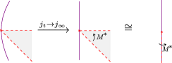
Figure 20: In a complex structure limit, the wall becomes straight. We can move the cut to the invariant direction of the monodromy, that is the same direction as the limit straight wall.

Remark 8

As described by Mikhalkin Mi04b , we can deform the complex structure on $X^{\vee}$ to a limit where holomorphic curves would converge to tropical curve on the base with respect to the so-called complex affine structure, which is dual to the symplectic affine structure. So, (relative) Gromov-Witten invariants of $X^{\vee}$ are expected to be described by tropical curves ($\vartheta$ functions) in the base $B$, with the affine structure describing $X_{\Lambda}$ (or $X_{\mathbb{C}}$). In particular, the wall becomes straight in this limit, as illustrated by Figure 20.

As we mentioned before, we will now replace the formal variable $T$ by $e^{-1}$ in our construction, and consider the mirror as the moduli of Lagrangian fibres endowed with $U(1)$-local systems. So, after completion the mirror becomes

$$X=X_{\mathbb{C}}=\{(u,v,w)\in\mathbb{C}^{2}\times\mathbb{C}^{*};uv=1+w\}$$

endowed with a completed symplectic form $\omega$ as described in (Au09, , Proposition 2.3). Its SYZ dual ATF (dual to the one on $X^{\vee}$) is then described by any of the diagrams in Figure 20.

Remark 9

As we take the completion, the $\mathrm{val}$ defined in $X_{\Lambda}$ approaches $-\log|.|$ defined in $X_{\mathbb{C}}$.

We see now that the rightmost diagram in Figure 20, can describe an ATF, and once decorated with wall crossing functions [$(1+w^{\pm 1})$ accordingly] along the wall, it can algebraically determine the space $X_{\mathbb{C}}$. The variety $X_{\mathbb{C}}$ is then built out of two $(\mathbb{C}^{*})^{2}$ charts, with coordinates $(u,w)$ and $(v,w)$, glued together in a cluster like transition birational map $uv=1+w$, defined in the complement of $\{w=-1\}$. A unique wall, decorated with such wall crossing function, describing $X_{\mathbb{C}}$ is the simplest version of a scattering diagram GS ; GHKlog (see Section 2 for more details).

The $A_{2}$ Cluster Variety: ATF and Scattering Diagram

As described in (ghkk, , Example 8.40) (taking the parameters $X_{1},X_{2}$ to be $1$), we describe the affine ($\vartheta_{0}=1$) $A_{2}$ Cluster variety by the ring in five variables $\vartheta_{i}$, $i=1,\dots,5$ satisfying the relations:

$$\vartheta_{1}\vartheta_{3}=1+\vartheta_{2}$$

$$\vartheta_{2}\vartheta_{4}=1+\vartheta_{3}$$

$$\vartheta_{3}\vartheta_{5}=1+\vartheta_{4}$$

$$\vartheta_{4}\vartheta_{1}=1+\vartheta_{5}$$

$$\vartheta_{5}\vartheta_{2}=1+\vartheta_{1}$$

We see that this variety is obtained by gluing five algebraic tori $(\mathbb{C}^{*})^{2}$, with coordinates $(\vartheta_{i},\vartheta_{i+1})$ [indices taken $\mod$ 5], according to the above cluster relations. We saw in more details in Section 2 that these relations are encoded by the data of a scattering diagram, as illustrated in the top-right picture of Figure 21.

Figure 21: Scattering diagram and ATF for the $A_{2}$ cluster variety.

Let’s start with the data of an ATF describing a symplectic manifold $X$, with 2 nodal fibres, whose monodromies are encoded by cuts pointing away from the nodes in the directions $(0,1)$ and $(-1,0)$, respectively, as illustrated in the bottom-left picture of Figure 21. We now think think of this as endowed with the completed infinite volume symplectic form, so the base diagram covers the whole $\mathbb{R}^{2}$. As indicated in the previous Section, to build complex charts on this space, we add one wall for each node, represented by a line in the invariant direction of the monodromy. [These walls represent dual fibres in the mirror $X^{\vee}$, bounding Maslov index 0 disks with respect to a limit complex structure $j_{\infty}$.] We call the chamber containing the nodes the main chamber, and we associate to it a complex torus $(\mathbb{C}^{*})^{2}$, with coordinates $(\vartheta_{2},\vartheta_{3})$, and associated with the corresponding wall is a gluing function of the form $(1+\vartheta_{i})$. One can check that changing coordinates around these 4 walls in a full circle, does not give you identity on the $(\vartheta_{2},\vartheta_{3})$ algebraic torus. To correct for that one needs to add an extra slab, in this case corresponding to a ray in direction $(1,-1)$, and a corresponding transition function giving you now $5$ chambers, each corresponding to an algebraic torus, as illustrated in the top-right picture of Figure 21. This collection of walls and slabs is called the scattering diagram GS [recall the details in Section 2]. This scattering diagram describe the relations of the $A_{2}$ cluster variety given in the beginning of this Section.

We can compactify this $A_{2}$ cluster variety by homogenizing its defining equations, as $\vartheta_{1}\vartheta_{3}=\vartheta_{0}^{2}+\vartheta_{2}\vartheta_{0},\dots,\vartheta_{5}\vartheta_{2}=\vartheta_{0}^{2}+\vartheta_{1}\vartheta_{0}$. As mentioned in (ghkk, , Example 8.40), this gives a del Pezzo surface of degree 5 in $\mathbb{C}P^{5}$. Intersecting the hyperplane $\vartheta_{0}=0$, we see a chained loop of 5 divisors. Symplectically, it is natural to endow the del Pezzo surface with the monotone symplectic form given by restricting the Fubini-Study form of $\mathbb{C}P^{5}$. The complement of the five above mentioned divisors can be seen as a (Weinstein) subdomain of $X$, whose completion give $X$. Indeed, there is an ATF on the degree 5 del Pezzo surface, as illustrated in the bottom-right diagram of Figure 21. [We can obtain this ATF by performing a monotone blowup in a corner of (Vi16a, , diagram $(A_{3})$ of Figure 16).] The chained loop of 5 divisors is identified with the boundary of this ATF, and the complement of them is a subdomain of $X$ as illustrated by the bottom-left diagram of Figure 21.

3.2 Compactifications of Cluster varieties

We saw in the previous section how to relate the data representing an almost-toric fibration in a open symplectic manifold with a set of initial walls, out of which Gross-Siebert GS explains how to complete to a scattering diagram that provides this manifold with complex charts given by gluing algebraic tori $(\mathbb{C}^{*})^{2}$ along the walls.

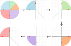
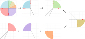
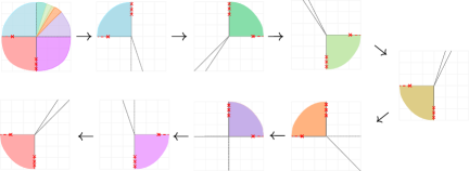
Figure 22: Cluster charts via symplectic mutations on affine cluster varieties

As mentioned in Section 2.1, we can construct cluster varieties out of this data, and we will focus on the varieties of finite type $A_{2}$, $B_{2}$, $G_{2}$. These are open exact almost toric manifolds, built out of the scattering diagram with initial data given by two orthogonal walls, one of them associated to one node and the other with one, two and three nodes, respectively, as indicated in Figure 22. Recall we call the chart containing all nodes the main chart. One sees that symplectic mutation can be associated to changing the main chart, as illustrated in Figure 22. In other words, without the prior knowledge, the scattering diagram can be recovered by keeping track of the “main charts” as we apply the corresponding mutations, as illustrated in Figure 22. [This is not the case when the scattering diagram has a dense regions of slabs. For instance, when considering the scattering diagram associated to the mirror of the complement of an elliptic curve in $\mathbb{C}\mathbb{P}^{2}$. Note that this case is considered in lin2020enumerative .]

In this section, we are interested in understanding compactifications of these cluster varieties from the symplectic perspective. Compact symplectic manifolds have finite volume, hence we will consider as $X$ a subdomain, whose completion is the manifold described by the ATF with base diagram covering the whole $\mathbb{R}^{2}$. We will consider equivalent the subdomains with same completion.

All the symplectic compactifications considered here are symplectic del Pezzos, in the sense that they are endowed with a monotone symplectic form, which is unique up to scaling and symplectomorphisms MD90 ; LiLiu95 ; OhtaOno96 ; OhtaOno97 . This ensures the existence of a monotone fibre, that can be detected by the intersection point of the lines in the diagrams that go through the nodes and are in the direction of the cuts. A symplectomorphism class invariant of these monotone fibres (the star-shape) is shown ShToVi18 to be given by the interior of the polytope seen in $H^{1}(T^{2},\mathbb{R})\cong\mathbb{R}^{2}$, as we forget the nodes and cuts. So there is a symplectomorphism identifying two monotone fibres of an ATF, if and only if, the associated polytopes are related under $\mathrm{SL}(2;\mathbb{Z})$. If there exists such ambient symplectomorphism, we say the Lagrangians are symplectomorphic.

In the definition of mutation of ATFs on del Pezzo surface Vi16a , besides mutating the polytope by changing the direction of the cut, it is required that we slide the cut through the monotone fibre. In that sense, we say that the corresponding monotone fibres are related by mutation. We can then form a graph with vertices representing symplectomorphism class of a Lagrangian and edges represented these Lagrangians being related by mutation. One aspect we can extract from the cyclic behaviour of these finite cluster varieties is the existence of cycles in the above mentioned graph. This behaviour does not appear in mutations of monotone almost toric fibres in $\mathbb{C}P^{2}$, and conjecturally in $\mathbb{C}P^{1}\times\mathbb{C}P^{1}$.

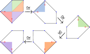
Figure 23: Mutations on degree 5 del Pezzo – 1 torus

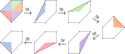
Figure 24: Mutations on degree 5 del Pezzo – 1 torus

Let us start looking at the example from Section 3.1 ((ghkk, , Example 8.40), (cpt, , Figure 1)), a compactification of the $A_{2}$ cluster variety to the degree 5 del Pezzo, by adding a chain of 5 divisors, whose union represents the anti-canonical class. This compactification and its mutations are illustrated in Figures 23, 24. Note that we get the same pattern as in Figures 6, 7, where we get back to the same picture after, respectively, 4 and 6 cycles, depending on the pattern of mutation. This is misleading, as ATFs, the mutations should not depend on which half-space is fixed, and which you decide to shear. In fact, in this example, all diagrams are ($SL(2;\mathbb{Z})$) equivalent, which in particular implies that the monotone tori in each pictures are mutually symplectomorphic. The 5-cycle pattern of the $A_{2}$ cluster appears by looking at the main charts, which we have already illustrated in Figure 22. In particular, this example does not give us a cycle of monotone Lagrangian tori, since we quotient out the graph associated to mutations by equivalence.

We want to extend a bit our notion of compactification. We will say that a (Weinstein) domain $X$ compactifies to $\overline{Y}$, if we have $X\subset Y\subset\overline{Y}$, with $X$ a sub-domain of $Y$ and $Y=\overline{Y}\setminus\bigcup_{i}D_{i}$, for symplectic divisors $D_{i}$. This will be used by us to identify our domains of interest, described in Figure 22, appearing as open pieces of ATFs in del Pezzo surfaces, where we do not include all the nodes. See for instance, Figures 26, 28, 32, 33. In these cases, our domain of interest $X$ is not the complement $Y$ of the symplectic divisors projecting over the boundary of the ATF, but rather a subdomain of $Y$. The nodes not contained in the ATF describing $X$ will be considered frozen (not used to mutate), and depicted as a blue $\times$.

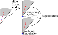
Figure 25: Moving frozen nodes to the boundary, is equivalent to have over the vertex a possibly singular Lagrangian representing a vanishing cycle of a degeneration to a toric orbifold singularity. This vanishing cycle is represented by a pentagon over the vertex, and the orbifold singularity by a star in the above diagrams. Up to equivalence, the shaded domain can be viewed either as a subdomain of the complement of the boundary divisors in the left-picture, or the complement of the singular divisors in the orbifold diagram.

An alternative way of thinking is to disregard the frozen nodes. The total manifold $\tilde{Y}$ becomes singular, and a non-smooth compactification of $X$, given by adding the boundary divisor. The singularities are orbifold $T$-singularities AkKa16 at each vertex, that were previously associated with the frozen nodes. Our original smooth manifold, that included the frozen nodes, is a smoothing of this orbifold. There is a continuous way of relating the Lagrangian fibrations on the orbifold with the ATF on the smoothing. We like to interpret it as a two step process, which is locally illustrated in Figure 25. The first, we keep the symplectic form on $\overline{Y}$, and consider almost-toric fibrations $ATF_{t}$, $t\in[0,1)$, so that in the limit $t\to 1$ the blue nodes slide all the way to a limit vertex at the boundary, and we are left with a singular Lagrangian fibration $SLF_{1}$, on $\overline{Y}$, such that over the limit vertices live a possibly singular Lagrangian. The Lagrangian over each limit vertex can be recognised in each $ATF_{t}$, $t<1$ living over the associated cut from the boundary of the ATF up to the farthest blue node and intersecting each fibre over the cut in a collapsing cycle for the corresponding nodes. This limit can be made rigorous but is beyond the scope of this article. The second step is to consider a degeneration from $\overline{Y}$ to $\tilde{Y}$, and a family of singular Lagrangian fibrations $SLF_{s}$, in the fibers corresponding to $s\in(0,1]$, where in the limit $s\to 0$ the singular Lagrangian over each vertex collapses to the corresponding orbifold singularity. The Lagrangian fibrations $SLF_{s}$ are identified under symplectic parallel transport, so the singular Lagrangian over each vertex degenerating to an orbifold singularity is precisely the vanishing cycle of that orbifold singularity. In the examples presented here, the singularities associated with the frozen nodes will always be of $A_{n}$ type, and hence the corresponding Lagrangian a chain of $n-1$ spheres.

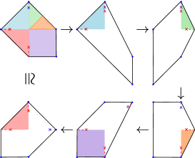
Figure 26: Mutations on degree 5 del Pezzo – 5 tori

Let’s turn our attention now to Figure 26, where we realize the degree 5 del Pezzo surface $\overline{Y}$ as a compactification of the $A_{2}$ cluster variety $X$, in a different way. We perform a nodal trade in a vertex at the bottom of the second diagram in Figure 23, and we freeze the top node. Now the boundary divisor represents 4 symplectic spheres, and $X$ is a subdomain of the complement of these divisors. In this case, the mutation cycle induced by the nodal singularities in $X$ does provides us with a 5-cycle of distinct monotone Lagrangian tori. Recall that monotone fibres of non-$SL(2,\mathbb{Z})$ related diagrams are distinct ShToVi18 .

Remark 10

Disregarding the frozen node creates a double point singularity. In contrast with (ghkk, , Example 8.40), this is the same as considering $X_{1}=0$ in their setting. Now, consider the cycle of 5 divisors given by $\vartheta_{0}=0$. We claim that if one smooths one node of this chain (represented by our nodal trade), and then delete the resulting chain of 4 divisors in this orbifold, one recovers $X$, the $A_{2}$ cluster variety.

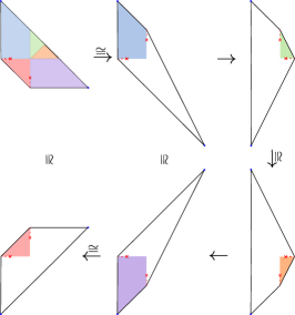
Figure 27: Mutations on degree 8 del Pezzo – 2 tori

We can see that there is a simpler compactification of the $A_{2}$ cluster variety $X$ by $\overline{Y}=\mathbb{C}P^{2}\#\overline{\mathbb{C}P^{2}}$, a degree 8 del Pezzo, as illustrated in Figure 27 [which is the same obtained in Figure 14]. Here, $X$ is the complement of two divisors in classes $H$ and $2H-E$, where $H$ is the class of the line, and $E$ is the exceptional class. Note that we do not get a cycle of monotone Lagrangian tori, though not all tori are equivalent, we only see 2 tori in the whole cycle, which gives us only an edge on the unoriented graph of mutations of monotone tori, modulo equivalence.

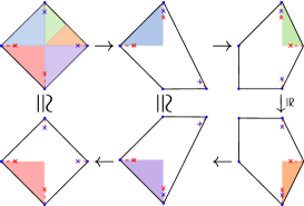
Figure 28: Mutations on degree 4 del Pezzo – 3 tori

Clearly, performing a blowup on one of the divisors of $\overline{Y}$ gives us another compactification of $X$. The top left diagram of Figure 28 corresponds to a toric blowup of monotone size [recall that in symplectic geometry, the blowups depend on the size of a symplectic ball one chooses to delete] in the top left diagram of either Figure 23 or Figure 26. Note in this case that the third and fourth, as well as the second and fifth, diagrams are equivalent, failing to deliver a cycle on the mutation graph of monotone Lagrangian tori in the degree 4 del Pezzo.

[scale= 0.35]dp6_mut_1_charts_gl.pdf

Figure 29: Mutations on degree 6 del Pezzo – 6 tori

Figure 30: This diagram differ from the sixth diagram in Figure 29, by one nodal trade and one inverse nodal trade. Mutations of the displayed nodes give equivalent polytopes.

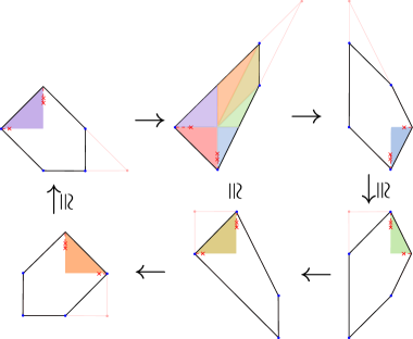
Figure 31: Mutations on degree 5 del Pezzo – 3 tori

Let us consider now $X$ the $B_{2}$ type cluster variety, with almost toric fibrations as in the series of diagrams in the middle of Figure 22. The first compactification $\overline{Y}$ we look at is the degree 6 del Pezzo, starting with the ATF depicted in the top-left diagram of Figure 29. [This diagram is $SL(2;\mathbb{Z})$ equivalent to (Vi16a, , Diagram $(A_{5})$, Figure 16) (up to nodal trades).] In this case $X$ is the complement of three divisors of $\overline{Y}=\mathbb{C}P^{2}\#3\overline{\mathbb{C}P^{2}}$, having symplectic areas 1, 2 and 3. We see that in this case we do get a cycle of size 6, with one torus corresponding to each cluster chart.

It is interesting to notice that the sixth diagram seems to have come from the scattering diagram Figure 16. But it is not quite the case, since that scattering diagram has a square function corresponding to the horizontal cut in the sixth diagram Figure 29, while a simple function corresponding to the vertical cut. This means that the natural compactification coming from that scattering diagram would be the same del Pezzo, but represented by the diagram of Figure 30 coming from applying a nodal trade to the corner associated to the horizontal cut in the sixth diagram Figure 29, and an inverse nodal trade on one node at the vertical cut. In particular, $X$ would be seen as the complement of 3 divisors in $\overline{Y}=\mathbb{C}P^{2}\#3\overline{\mathbb{C}P^{2}}$, each of symplectic area 2. The reader can check that in this case, the mutations associated to $X$ would give equivalent monotone Lagrangian tori, analogous to the previous case depicted in Figures 23, 24.

Clearly we can also compactify the $B_{2}$ type cluster variety $X$ to the degree 5 del Pezzo, as the complement of four divisors as depicted in Figure 31, by simply applying a nodal trade to a diagram in Figure 23. In Figure 31, we depicted segments outside the diagrams to indicate that they come from applying blowups to the diagrams in Figure 29. Curiously, it behaves similarly to the case in Figure 28, where we have only three non-equivalent Lagrangian tori, not providing a cycle.

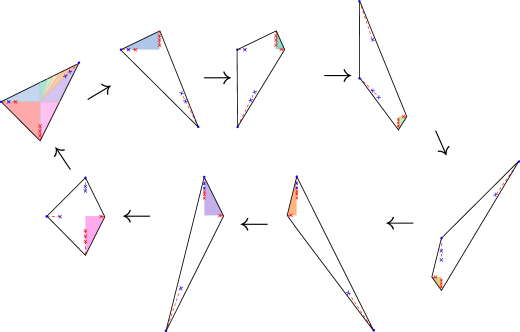
Figure 32: Mutations on degree 3 del Pezzo – 8 tori

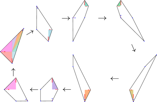
Figure 33: Mutations on degree 4 del Pezzo – 8 tori

We now finish by presenting two compactifications of the $G_{2}$ cluster variety. We name it $X$, and consider it as an almost toric variety corresponding to the bottom series of diagrams in Figure 22. We start noting that the compactifications described in cpt , see for instance (cpt, , Figure 18), seems to be giving partially, but not fully, smoothable orbifolds. Here we look to two compactifications to degree 3 and 4 del Pezzo surfaces. [Both contain frozen variables, so the reader may prefer the alternative idea of seeing $X$ compactifying to a degeneration of these surfaces.]

We start with the top left ATBD in Figure 32, which is equivalent to (Vi16a, , Diagram $(B_{2})$, Figure 19), representing an ATF of the cubic $\mathbb{C}P^{2}\#6\overline{\mathbb{C}P^{2}}$. In this case, $X$ is a subdomain of the complement of two symplectic divisors. Sliding the frozen nodes to the corresponding vertex gives one Lagrangian sphere, in the horizontal cut, and a chain of two Lagrangian spheres in $(1,1)$-cut. This indicates that disregarding the frozen nodes corresponds to considering an orbifold with one double-point singularity and one triple-point singularity. We do get one monotone Lagrangian torus for each of the 8 cluster charts in this case.

Another compactification of $X$ is given in Figure 33. The top left diagram of Figure 33 is equivalent (up to nodal trades) to (Vi16a, , Diagram $(B_{2})$, Figure 18). Here, $X$ is viewed as a subdomain of the complement of three symplectic divisors in $\overline{Y}=\mathbb{C}P^{2}\#5\overline{\mathbb{C}P^{2}}$. Sliding the frozen node to the vertex provides Lagrangian sphere, or equivalently, disregarding the node gives a double-point orbifold singularity at the vertex. As before, we get one monotone Lagrangian torus for each cluster chart.

References

- (1) Akhtar, M., Coates, T., Galkin, S., Kasprzyk, A.M.: Minkowski polynomials and mutations. SIGMA Symmetry Integrability Geom. Methods Appl. 8, Paper 094, 17 (2012)
- (2) Akhtar, M.E., Kasprzyk, A.M.: Mutations of fake weighted projective planes. Proc. Edinb. Math. Soc. (2) 59(2), 271–285 (2016)
- (3) Arnold́, V.I.: Mathematical methods of classical mechanics, Graduate Texts in Mathematics, vol. 60. Springer-Verlag, New York (1989). Translated from the 1974 Russian original by K. Vogtmann and A. Weinstein, Corrected reprint of the second (1989) edition
- (4) Auroux, D.: Mirror symmetry and T-duality in the complement of an anticanonical divisor. J. Gökova Geom. Topol. 1, 51–91 (2007)
- (5) Auroux, D.: Special Lagrangian fibrations, wall-crossing, and mirror symmetry. In: Surveys in differential geometry. Vol. XIII. Geometry, analysis, and algebraic geometry: forty years of the Journal of Differential Geometry, Surv. Differ. Geom., vol. 13, pp. 1–47. Int. Press, Somerville, MA (2009). DOI 10.4310/SDG.2008.v13.n1.a1
- (6) Cheung, M.W., Lin, Y.S.: Some examples of Family Floer mirror. arXiv preprint arXiv:2101.07079 (2021)
- (7) Cheung, M.W., Magee, T.: Towards Batyrev duality for finite-type cluster varieties. In preparation
- (8) Cheung, M.W., Magee, T., Nájera-Chávez, A.: Compactifications of cluster varieties and convexity. To appear in International Mathematics Research Notices
- (9) Collins, T., Jacob, A., Lin, Y.S.: Special lagrangian submanifolds of log calabi-yau manifolds
- (10) Eliashberg, Y., Polterovich, L.: Unknottedness of Lagrangian surfaces in symplectic -manifolds. Internat. Math. Res. Notices (11), 295–301 (1993). DOI 10.1155/S1073792893000339. URL http://dx.doi.org/10.1155/S1073792893000339
- (11) Fock, V., Goncharov, A.B.: Cluster ensembles, quantization and the dilogarithm. Annales scientifiques de l’École Normale Supérieure 42(6), 865–930 (2009)
- (12) Fomin, S., Zelevinsky, A.: Cluster algebras I: Foundations. J. Amer. Math. Soc. 15, 497––529 (2002)
- (13) Galkin, S., Usnich, A.: Laurent phenomenon for landau-ginzburg potential (2010). Available at http://research.ipmu.jp/ipmu/sysimg/ipmu/417.pdf
- (14) Gross, M.: Special Lagrangian fibrations. I: Topology. AMS/IP Stud. Adv. Math. 23, 65–93 (2001)
- (15) Gross, M., Hacking, P., Keel, S.: Mirror symmetry for log Calabi-Yau surfaces I. Publications mathématiques de l’IHÉS pp. 1–104 (2011)
- (16) Gross, M., Hacking, P., Keel, S.: Birational geometry of cluster algebras. Algebraic Geometry 2(2), 137–175 (2015)
- (17) Gross, M., Hacking, P., Keel, S., Kontsevich, M.: Canonical bases for cluster algebras. Journal of the American Mathematical Society 31(2), 497–608 (2018)
- (18) Gross, M., Hacking, P., Keel, S., Siebert, B.: The mirror of the cubic surface. arXiv preprint arXiv:1910.08427 (2019)
- (19) Gross, M., Siebert, B.: From real affine geometry to complex geometry. Annals of mathematics 174(3), 1301–1428 (2011)
- (20) Gross, M., Siebert, B.: Intrinsic mirror symmetry. arXiv preprint arXiv:1909.07649 (2019)
- (21) Kontsevich, M., Soibelman, Y.: Affine structures and non-Archimedean analytic spaces. In: The unity of mathematics, Progr. Math., vol. 244, pp. 321–385. Birkhäuser Boston (2006)
- (22) Leung, N.C., Symington, M.: Almost toric symplectic four-manifolds. J. Symplectic Geom. 8(2), 143–187 (2010)
- (23) Li, T.J., Liu, A.: Symplectic structure on ruled surfaces and a generalized adjunction formula. Math. Res. Lett. 2(4), 453–471 (1995). DOI 10.4310/MRL.1995.v2.n4.a6. URL https://doi.org/10.4310/MRL.1995.v2.n4.a6
- (24) Lin, Y.S.: Enumerative geometry of del pezzo surfaces. arXiv preprint arXiv:2005.08681 (2020)
- (25) Mandel, T.: Tropical theta functions and log calabi–yau surfaces. Selecta Mathematica 22(3), 1289–1335 (2016)
- (26) McDuff, D.: The structure of rational and ruled symplectic -manifolds. J. Amer. Math. Soc. 3(3), 679–712 (1990). DOI 10.2307/1990934. URL http://dx.doi.org/10.2307/1990934
- (27) Mikhalkin, G.: Amoebas of algebraic varieties and tropical geometry. In: Different faces of geometry, Int. Math. Ser. (N. Y.), vol. 3, pp. 257–300. Kluwer/Plenum, New York (2004)
- (28) Ohta, H., Ono, K.: Notes on symplectic -manifolds with . II. Internat. J. Math. 7(6), 755–770 (1996). DOI 10.1142/S0129167X96000402. URL http://dx.doi.org/10.1142/S0129167X96000402
- (29) Ohta, H., Ono, K.: Symplectic -manifolds with . In: Geometry and physics (Aarhus, 1995), Lecture Notes in Pure and Appl. Math., vol. 184, pp. 237–244. Dekker, New York (1997)
- (30) Shelukhin, E., Tonkonog, D., Vianna, R.: Geometry of symplectic flux and Lagrangian torus fibrations. arXiv:1804.02044 (2018)
- (31) Strominger, A., Yau, S.T., Zaslow, E.: Mirror symmetry is -duality. Nuclear Phys. B 479(1-2), 243–259 (1996). DOI 10.1016/0550-3213(96)00434-8. URL http://dx.doi.org/10.1016/0550-3213(96)00434-8
- (32) Symington, M.: Four dimensions from two in symplectic topology. In: Topology and geometry of manifolds (Athens, GA, 2001), Proc. Sympos. Pure Math., vol. 71, pp. 153–208. Amer. Math. Soc., Providence, RI (2003)
- (33) Vianna, R.: Infinitely many exotic monotone Lagrangian tori in . J. Topol. 9(2), 535–551 (2016)
- (34) Vianna, R.: Infinitely many monotone Lagrangian tori in del Pezzo surfaces. Selecta Math. (N.S.) 23(3), 1955–1996 (2017)