LCTP-20-18


Universal Logarithmic Behavior in Microstate Counting


and the Dual One-loop Entropy of AdS4 Black Holes


Leopoldo A. Pando Zayasa,b and Yu Xinc


a Leinweber Center for Theoretical Physics, Randall Laboratory of Physics

The University of Michigan, Ann Arbor, MI 48109-1120


b The Abdus Salam International Centre for Theoretical Physics

Strada Costiera 11, 34151 Trieste, Italy


c Department of Applied Mathematics and Theoretical Physics,

University of Cambridge, Cambridge, CB3 0WA, UK


We numerically study the topologically twisted index of several three-dimensional supersymmetric field theories on a genus g𝑔g Riemann surface times a circle, Σg×S1subscriptΣ𝑔superscript𝑆1\Sigma_{g}\times S^{1}. We show that for a large class of theories with leading term of the order N3/2superscript𝑁32N^{3/2}, where N𝑁N is generically the rank of the gauge group, there is a universal logarithmic correction of the form g12logN𝑔12𝑁\frac{g-1}{2}\log N. We explain how this logarithmic subleading correction can be obtained as a one-loop effect on the dual supergravity theory for magnetically charged, asymptotically AdS×4M7{}_{4}\times M^{7} black holes for a large class of Sasaki-Einstein manifolds, M7superscript𝑀7M^{7}. The matching of the logarithmic correction relies on a generic cohomological property of M7superscript𝑀7M^{7} and it is independent of the black hole charges. We argue that our supergravity results apply also to rotating, electrically charged asymptotically AdS×4M7{}_{4}\times M^{7} black holes. We present explicitly the quiver gauge theories and the gravity side corresponding to M7=N0,1,0,V5,2superscript𝑀7superscript𝑁010superscript𝑉52M^{7}=N^{0,1,0},V^{5,2} and Q1,1,1superscript𝑄111Q^{1,1,1}.


lpandoz@umich.edu, yx328@cam.ac.uk

1 Introduction

One remarkable recent result in the context of the AdS/CFT correspondence is the microscopic understanding of the Bekenstein-Hawking entropy of a class of asymptotically AdS4 black holes. Benini, Hristov and Zaffaroni demonstrated in [1] that the topologically twisted index of ABJM theory reproduces the entropy of the dual magnetically charged, asymptotically AdS×4S7{}_{4}\times S^{7} black holes.

Similar microscopic foundations via the topologically twisted index were provided for the corresponding macroscopic black hole entropy in different situations, including: dyonic black holes [2], black holes with hyperbolic horizons [3] and asymptotically AdS4 black holes in massive IIA supergravity [4, 5]. Some interesting progress has also been reported in the higher dimensional context [6, 7, 8, 9, 10] and for AdS4 black holes embeddable in certain universal sectors of M2 [11] and M5 backgrounds [12, 13] (see [14, 15] for reviews and a complete list of references for those developments). An analogous microscopic description, rooted in the superconformal index, has recently been presented for rotating, electrically charged AdS4 black holes [16, 17], including in a universal sector arising from wrapped M5 branes [18, 19].

The robust agreement at the leading order inspired attempts to understand the topologically twisted index beyond the large N𝑁N limit with focus on the logarithmic corrections to the entropy on both sides of the correspondence [20, 21]. The initial conclusion, however, was that more work was required and that Sen’s quantum entropy formalism in its current formulation needed to be amended to also account for hair degrees of freedom away from the near-horizon region. Ultimately, precise agreement was found in [22] whose computation focused on the asymptotically AdS4 region of the black hole solution. Further successful matches of the logarithmic contributions were provided in the case of universally embedded black holes [13, 19]. This subleading agreement motivates us to embark on a systematic exploration of a large class of models with the aim of demonstrating that the logarithmic correction is, indeed, quite universal. This is precisely one of the main results of this paper: an expression for the logarithmic corrections of the topologically twisted index for a large class of field theories on Σg×S1subscriptΣ𝑔superscript𝑆1\Sigma_{g}\times S^{1}, which we find to be g12logN𝑔12𝑁\frac{g-1}{2}\log N.

Let us describe two important previous results that make the journey to a universal logarithmic correction plausible. The first precedent pointing to the fact that the coefficient of logN𝑁\log N in the topologically twisted index could be universal comes from a subleading analysis of the free energy of a large class of 3d field theories. The exact partition function for a large class of Chern-Simons matter theories on S3superscript𝑆3S^{3} can be computed using field theory localization and certain matrix model techniques, the answer can be succinctly written in terms of an Airy function [23]. In some cases the supergravity dual is known to be a background of M-theory on AdS×4M7{}_{4}\times M^{7}, where M7superscript𝑀7M^{7} is a Sasaki-Einstein seven-dimensional manifold. The universality of the logarithmic term in the free energy on S3superscript𝑆3S^{3} established in [23] was beautifully elucidated from the dual supergravity point of view in [24] and shown to depend on some mild cohomological properties of the seven-dimensional manifold M7superscript𝑀7M^{7}. Some of our arguments in this manuscript mimic that analysis closely. The other important source of inspiration for us is a group of works that established a leading order in N𝑁N relationship between the free energy on S3superscript𝑆3S^{3} and the topologically twisted index on S2×S1superscript𝑆2superscript𝑆1S^{2}\times S^{1} presented and developed in [25, 26]. There is a formal background that arguably provides a rigorous basis for relations among the free energy on S3superscript𝑆3S^{3} and the topologically twisted index in Σg×S1subscriptΣ𝑔superscript𝑆1\Sigma_{g}\times S^{1} [27, 28, 12, 29] but we were particularly inspired by the two developments mentioned above. In this manuscript we effectively ask the questions of whether there is a relationship between the free energy on S3superscript𝑆3S^{3} and the topologically twisted index in Σg×S1subscriptΣ𝑔superscript𝑆1\Sigma_{g}\times S^{1} beyond the leading order in N𝑁N and, in particular, whether we can establish the universality of the logarithmic in N𝑁N correction. We are not able to answer the broader question of the relationship between the free energy on S3superscript𝑆3S^{3} and the topologically twisted index beyond the large N𝑁N limit but we present strong numerical evidence in favor of a universal logarithmic correction in the topologically twisted index very similar to the universality of the logarithmic term for the free energy.

The rest of the manuscript is organized as follows. We start in section 2 by briefly reviewing the topologically twisted index in general and its form for the ABJM theory. Sections 3, 4 and 5 are devoted to extensive numerical evaluations of the topologically twisted index for the 3d Chern-Simons matter theories dual to M-theory on AdS×4M7{}_{4}\times M^{7} for M7=N0,1,0,V5,2,Q1,1,1superscript𝑀7superscript𝑁010superscript𝑉52superscript𝑄111M^{7}=N^{0,1,0},V^{5,2},Q^{1,1,1}, respectively. We discuss the one-loop gravity computation dual to the universal result in section 6. We conclude in section 7 where we also point to a number of interesting, in our opinion, open problems.

2 The topologically twisted index for generic 𝒩=2𝒩2{\cal N}=2 theories

In this section we will briefly review the construction and structure of the topologically twisted index for 3d 𝒩=2𝒩2{\cal N}=2 supersymmetric theories. The topologically twisted index for three dimensional 𝒩=2𝒩2{\cal N}=2 field theories was defined in [30] (see other related works [31, 32, 25, 26, 33]) by evaluating the supersymmetric partition function on S1×S2superscript𝑆1superscript𝑆2S^{1}\times S^{2} with a topological twist on S2superscript𝑆2S^{2}. One considers a 3d theory, usually containing Yang-Mills, YMsubscript𝑌𝑀{\cal L}_{YM}, and Chern-Simons, CSsubscript𝐶𝑆{\cal L}_{CS}, interactions on S2×S1superscript𝑆2superscript𝑆1S^{2}\times S^{1} with metric and background field given as

ds2=R2(dθ2+sin2θdϕ2)+β2dt2,AR=12cosθdϕ.formulae-sequence𝑑superscript𝑠2superscript𝑅2𝑑superscript𝜃2superscript2𝜃𝑑superscriptitalic-ϕ2superscript𝛽2𝑑superscript𝑡2superscript𝐴𝑅12𝜃𝑑italic-ϕds^{2}=R^{2}(d\theta^{2}+\sin^{2}\theta d\phi^{2})+\beta^{2}dt^{2},\qquad A^{R}=\frac{1}{2}\cos\theta d\phi. (2.1)

There is typically a set of flavor symmetries characterized by Cartan-valued magnetic fluxes:

Jf=12πS2Ff=𝔫.superscript𝐽𝑓12𝜋subscriptsuperscript𝑆2superscript𝐹𝑓𝔫J^{f}=\frac{1}{2\pi}\int_{S^{2}}F^{f}=\mathfrak{n}. (2.2)

With these magnetic fluxes one associates flavor fugacities y=exp[i(Atf+iβσf)]𝑦𝑖superscriptsubscript𝐴𝑡𝑓𝑖𝛽superscript𝜎𝑓y=\exp\left[i\left(A_{t}^{f}+i\beta\sigma^{f}\right)\right], where the constant potential Atfsuperscriptsubscript𝐴𝑡𝑓A_{t}^{f} is a flat connection for the flavor symmetry and σfsuperscript𝜎𝑓\sigma^{f} is a real mass for the three-dimensional field theory. Similarly the fugacities for the dynamical fields are x=exp[i(At+iβσ)]𝑥𝑖subscript𝐴𝑡𝑖𝛽𝜎x=\exp\left[i\left(A_{t}+i\beta\sigma\right)\right], where Atsubscript𝐴𝑡A_{t} runs over the maximal torus of the gauge group and σ𝜎\sigma over the corresponding Cartan subalgebra.

The topologically twisted index generically takes the from

Z(𝔫,y)=1|W|𝔪Γ𝔥𝒞Zint(x,y;𝔪,𝔫).𝑍𝔫𝑦1𝑊subscript𝔪subscriptΓ𝔥subscriptcontour-integral𝒞subscript𝑍𝑖𝑛𝑡𝑥𝑦𝔪𝔫Z(\mathfrak{n},y)=\frac{1}{|W|}\sum\limits_{\mathfrak{m}\in\Gamma_{\mathfrak{h}}}\oint_{\cal C}Z_{int}(x,y;\mathfrak{m},\mathfrak{n}). (2.3)

There is an algorithmic way of constructing Zintsubscript𝑍𝑖𝑛𝑡Z_{int} depending on the field content of the theory. Let us define the building blocks that go into Zintsubscript𝑍𝑖𝑛𝑡Z_{int}. For a chiral multiplet

Z1loopchiral=ρ(xρ/2yρf/21xρyρf)ρ(𝔪)+ρf(𝔫)q+1,superscriptsubscript𝑍1𝑙𝑜𝑜𝑝𝑐𝑖𝑟𝑎𝑙subscriptproduct𝜌superscriptsuperscript𝑥𝜌2superscript𝑦subscript𝜌𝑓21superscript𝑥𝜌superscript𝑦subscript𝜌𝑓𝜌𝔪subscript𝜌𝑓𝔫𝑞1Z_{1-loop}^{chiral}=\prod\limits_{\rho\in{\mathfrak{R}}}\left(\frac{x^{\rho/2}y^{\rho_{f}/2}}{1-x^{\rho}y^{\rho_{f}}}\right)^{\rho(\mathfrak{m})+\rho_{f}(\mathfrak{n})-q+1}, (2.4)

where {\mathfrak{R}} is the representation of the gauge group G𝐺G, ρ𝜌\rho denote the corresponding weights, q𝑞q is the R-charge of the field and ρfsubscript𝜌𝑓\rho_{f} is the weight of the multiplet under the flavor symmetry group. For the gauge multiplet one has

Z1loopgauge=αG(1xα)(idu)r,superscriptsubscript𝑍1𝑙𝑜𝑜𝑝𝑔𝑎𝑢𝑔𝑒subscriptproduct𝛼𝐺1superscript𝑥𝛼superscript𝑖𝑑𝑢𝑟Z_{1-loop}^{gauge}=\prod\limits_{\alpha\in G}(1-x^{\alpha})\left(idu\right)^{r}, (2.5)

where r𝑟r is the rank of the gauge group and α𝛼\alpha donate the roots of G𝐺G. We also use u=At+iβσ𝑢subscript𝐴𝑡𝑖𝛽𝜎u=A_{t}+i\beta\sigma which lives on the complexified Cartan subalgebra, essentially, x=eiu𝑥superscript𝑒𝑖𝑢x=e^{iu}.

The only classical contribution to Zintsubscript𝑍𝑖𝑛𝑡Z_{int} comes from the Chern-Simons term and takes the form

ZclassCS=xk𝔪,superscriptsubscript𝑍𝑐𝑙𝑎𝑠𝑠𝐶𝑆superscript𝑥𝑘𝔪Z_{class}^{CS}=x^{k\mathfrak{m}}, (2.6)

where k𝑘k is the Chern-Simons level and 𝔪𝔪\mathfrak{m} is the magnetic flux taking values in the co-root latice Γ𝔥subscriptΓ𝔥\Gamma_{\mathfrak{h}} of the gauge group. There is also the contribution of a U(1)𝑈1U(1) topological symmetry with holonomy ξ=eiz𝜉superscript𝑒𝑖𝑧\xi=e^{iz} and flux 𝔱𝔱\mathfrak{t}:

Zclasstop=x𝔱ξ𝔪.subscriptsuperscript𝑍𝑡𝑜𝑝𝑐𝑙𝑎𝑠𝑠superscript𝑥𝔱superscript𝜉𝔪Z^{top}_{class}=x^{\mathfrak{t}}\xi^{\mathfrak{m}}. (2.7)

With these ingredients one has that the index takes the general form

Z(𝔫,y)=1|W|𝔪Γ𝔥𝒞Cartan(dx2πixxk𝔪)αG(1xα)IρII(xρI/2yI1/21xρIyI)ρI(𝔪)𝔫I+1,𝑍𝔫𝑦1𝑊subscript𝔪subscriptΓ𝔥subscriptcontour-integral𝒞subscriptproductCartan𝑑𝑥2𝜋𝑖𝑥superscript𝑥𝑘𝔪subscriptproduct𝛼𝐺1superscript𝑥𝛼subscriptproduct𝐼subscriptproductsubscript𝜌𝐼subscript𝐼superscriptsuperscript𝑥subscript𝜌𝐼2superscriptsubscript𝑦𝐼121superscript𝑥subscript𝜌𝐼subscript𝑦𝐼subscript𝜌𝐼𝔪subscript𝔫𝐼1Z(\mathfrak{n},y)=\frac{1}{|W|}\sum\limits_{\mathfrak{m}\in\Gamma_{\mathfrak{h}}}\oint_{\cal C}\prod\limits_{{\rm Cartan}}\left(\frac{dx}{2\pi ix}x^{k\mathfrak{m}}\right)\prod\limits_{\alpha\in G}(1-x^{\alpha})\prod\limits_{I}\prod\limits_{\rho_{I}\in\mathfrak{R}_{I}}\left(\frac{x^{\rho_{I}/2}y_{I}^{1/2}}{1-x^{\rho_{I}}y_{I}}\right)^{\rho_{I}(\mathfrak{m})-\mathfrak{n}_{I}+1}, (2.8)

where α𝛼\alpha are the roots of G𝐺G, ρIsubscript𝜌𝐼\rho_{I} are the weights of the representation Isubscript𝐼\mathfrak{R}_{I} and 𝔪𝔪\mathfrak{m} are gauge magnetic fluxes living in the co-root lattice Γ𝔥subscriptΓ𝔥\Gamma_{\mathfrak{h}}.

The index depends on a choice of fugacities yIsubscript𝑦𝐼y_{I} for the flavor group and a choice of integer magnetic charges 𝔫Isubscript𝔫𝐼\mathfrak{n}_{I} for the R-symmetry of the theory. Both yIsubscript𝑦𝐼y_{I} and 𝔫Isubscript𝔫𝐼\mathfrak{n}_{I} are parameterized by the global symmetries of the theory. Each monomial term W𝑊W in the superpotential imposes a constraint:

IWyI=1,IW𝔫I=2,formulae-sequencesubscriptproduct𝐼𝑊subscript𝑦𝐼1subscriptproduct𝐼𝑊subscript𝔫𝐼2\prod\limits_{I\in W}y_{I}=1,\qquad\prod\limits_{I\in W}\mathfrak{n}_{I}=2, (2.9)

where the product and sum are restricted to the fields entering in W𝑊W. These constraints are called the marginality conditions of the superpotential.

After summing over the magnetic fluxes, 𝔪𝔪\mathfrak{m}, in Eq. (2.8), one obtains an expression for the index whose poles are located at positions determined by the following Bethe-Ansatz like expression

exp(isign(ka)Bi(a))=1.𝑖signsubscript𝑘𝑎subscriptsuperscript𝐵𝑎𝑖1\exp\left(i\,{\rm sign}(k_{a})B^{(a)}_{i}\right)=1. (2.10)

For the class of theories we are interested in this manuscript it is convenient to consider some representations explicitly. The ingredients in the topologically twisted index that we will require are:

  • The Vandermonde determinant contributes to the logarithm of the index as

    logij(1xi(a)xj(a))subscriptproduct𝑖𝑗1superscriptsubscript𝑥𝑖𝑎superscriptsubscript𝑥𝑗𝑎\displaystyle\log\prod\limits_{i\neq j}\left(1-\frac{x_{i}^{(a)}}{x_{j}^{(a)}}\right) =\displaystyle= logi<j(1xj(a)xi(a))2(xi(a)xj(a))subscriptproduct𝑖𝑗superscript1superscriptsubscript𝑥𝑗𝑎superscriptsubscript𝑥𝑖𝑎2superscriptsubscript𝑥𝑖𝑎superscriptsubscript𝑥𝑗𝑎\displaystyle\log\prod\limits_{i<j}\left(1-\frac{x_{j}^{(a)}}{x_{i}^{(a)}}\right)^{2}\left(-\frac{x_{i}^{(a)}}{x_{j}^{(a)}}\right) (2.11)
    =\displaystyle= ii<jN(ui(a)uj(a)+π)2i<jNLi1(ei(uj(a)ui(a))).𝑖superscriptsubscript𝑖𝑗𝑁superscriptsubscript𝑢𝑖𝑎superscriptsubscript𝑢𝑗𝑎𝜋2superscriptsubscript𝑖𝑗𝑁subscriptLi1superscript𝑒𝑖superscriptsubscript𝑢𝑗𝑎superscriptsubscript𝑢𝑖𝑎\displaystyle i\sum\limits_{i<j}^{N}(u_{i}^{(a)}-u_{j}^{(a)}+\pi)-2\sum\limits_{i<j}^{N}{\rm Li}_{1}\left(e^{i(u_{j}^{(a)}-u_{i}^{(a)})}\right).
  • The topological symmetry contributes as

    ii=1Nui(a)𝔱a,𝑖superscriptsubscript𝑖1𝑁superscriptsubscript𝑢𝑖𝑎subscript𝔱𝑎i\sum\limits_{i=1}^{N}u_{i}^{(a)}\mathfrak{t}_{a}, (2.12)

    where 𝔱asubscript𝔱𝑎\mathfrak{t}_{a} is the flux of the U(1)a𝑈subscript1𝑎U(1)_{a} topological symmetry.

  • A bi-fundamental chiral multiplet transforming in (𝐍¯,𝐍)¯𝐍𝐍(\bar{\bf N},{\bf N}) of U(N)a×U(N)b𝑈subscript𝑁𝑎𝑈subscript𝑁𝑏U(N)_{a}\times U(N)_{b} with magnetic flux 𝔫(b,a)subscript𝔫𝑏𝑎\mathfrak{n}_{(b,a)} and chemical potential Δ(b,a)subscriptΔ𝑏𝑎\Delta_{(b,a)} contributes as

    i=1N(xi(a)xi(b))12(𝔫(b,a)1)(1y(b,a)xi(b)xi(a))𝔫(b,a)1superscriptsubscriptproduct𝑖1𝑁superscriptsuperscriptsubscript𝑥𝑖𝑎superscriptsubscript𝑥𝑖𝑏12subscript𝔫𝑏𝑎1superscript1subscript𝑦𝑏𝑎superscriptsubscript𝑥𝑖𝑏superscriptsubscript𝑥𝑖𝑎subscript𝔫𝑏𝑎1\displaystyle\prod\limits_{i=1}^{N}\left(\frac{x_{i}^{(a)}}{x_{i}^{(b)}}\right)^{\frac{1}{2}(\mathfrak{n}_{(b,a)}-1)}\left(1-y_{(b,a)}\frac{x_{i}^{(b)}}{x_{i}^{(a)}}\right)^{\mathfrak{n}_{(b,a)}-1}
    ×\displaystyle\times i<jN(1)𝔫(b,a)1(xi(a)xi(b)xj(a)xj(b))12(𝔫(b,a)1)(1y(b,a)xj(b)xi(a))𝔫(b,a)1(1y(b,a)1xj(a)xi(b))𝔫(b,a)1.superscriptsubscriptproduct𝑖𝑗𝑁superscript1subscript𝔫𝑏𝑎1superscriptsuperscriptsubscript𝑥𝑖𝑎superscriptsubscript𝑥𝑖𝑏superscriptsubscript𝑥𝑗𝑎superscriptsubscript𝑥𝑗𝑏12subscript𝔫𝑏𝑎1superscript1subscript𝑦𝑏𝑎superscriptsubscript𝑥𝑗𝑏superscriptsubscript𝑥𝑖𝑎subscript𝔫𝑏𝑎1superscript1superscriptsubscript𝑦𝑏𝑎1superscriptsubscript𝑥𝑗𝑎superscriptsubscript𝑥𝑖𝑏subscript𝔫𝑏𝑎1\displaystyle\prod\limits_{i<j}^{N}(-1)^{\mathfrak{n}_{(b,a)}-1}\left(\frac{x_{i}^{(a)}x_{i}^{(b)}}{x_{j}^{(a)}x_{j}^{(b)}}\right)^{\frac{1}{2}(\mathfrak{n}_{(b,a)}-1)}\left(1-y_{(b,a)}\frac{x_{j}^{(b)}}{x_{i}^{(a)}}\right)^{\mathfrak{n}_{(b,a)}-1}\left(1-y_{(b,a)}^{-1}\frac{x_{j}^{(a)}}{x_{i}^{(b)}}\right)^{\mathfrak{n}_{(b,a)}-1}.
  • Fundamental and anti-fundamental fields contribute as

    logi=1Nantifundamentala(xi(a))12(𝔫~a1)[1y~a(xi(a))1]𝔫~a1superscriptsubscriptproduct𝑖1𝑁subscriptproductantifundamental𝑎superscriptsuperscriptsubscript𝑥𝑖𝑎12subscript~𝔫𝑎1superscriptdelimited-[]1subscript~𝑦𝑎superscriptsuperscriptsubscript𝑥𝑖𝑎1subscript~𝔫𝑎1\displaystyle\log\prod\limits_{i=1}^{N}\prod_{\begin{subarray}{c}{\rm anti-fundamental}\\ a\end{subarray}}\left(x_{i}^{(a)}\right)^{\frac{1}{2}(\tilde{\mathfrak{n}}_{a}-1)}\big{[}1-\tilde{y}_{a}\left(x_{i}^{(a)}\right)^{-1}\big{]}^{\tilde{\mathfrak{n}}_{a}-1} (2.14)
    ×\displaystyle\times fundamentala(xi(a))12(𝔫a1)[1ya1(xi(a))1]𝔫a1.subscriptproductfundamental𝑎superscriptsuperscriptsubscript𝑥𝑖𝑎12subscript𝔫𝑎1superscriptdelimited-[]1superscriptsubscript𝑦𝑎1superscriptsuperscriptsubscript𝑥𝑖𝑎1subscript𝔫𝑎1\displaystyle\prod_{\begin{subarray}{c}{\rm fundamental}\\ a\end{subarray}}\left(x_{i}^{(a)}\right)^{\frac{1}{2}(\mathfrak{n}_{a}-1)}\big{[}1-y_{a}^{-1}\left(x_{i}^{(a)}\right)^{-1}\big{]}^{\mathfrak{n}_{a}-1}.
  • As anticipated above, the contour integration is best expressed in terms of the position of the poles, given by the BA equation in terms of Bisubscript𝐵𝑖B_{i}. In taking the residues from one set of variables xisubscript𝑥𝑖x_{i} to another Bisubscript𝐵𝑖B_{i}, we incur a Jacobian denoted by 𝔹𝔹\mathbb{B}:

    𝔹=(eiBj(a),eiBj(b))(logxl(a),logxl(b))=(xl(a)eiBj(a)xl(a)xl(b)eiBj(a)xl(b)xl(a)eiBj(b)xl(a)xl(b)eiBj(b)xl(b))2N×2N,𝔹superscript𝑒𝑖subscriptsuperscript𝐵𝑎𝑗superscript𝑒𝑖superscriptsubscript𝐵𝑗𝑏superscriptsubscript𝑥𝑙𝑎superscriptsubscript𝑥𝑙𝑏subscriptsuperscriptsubscript𝑥𝑙𝑎superscript𝑒𝑖superscriptsubscript𝐵𝑗𝑎superscriptsubscript𝑥𝑙𝑎superscriptsubscript𝑥𝑙𝑏superscript𝑒𝑖superscriptsubscript𝐵𝑗𝑎superscriptsubscript𝑥𝑙𝑏superscriptsubscript𝑥𝑙𝑎superscript𝑒𝑖superscriptsubscript𝐵𝑗𝑏superscriptsubscript𝑥𝑙𝑎superscriptsubscript𝑥𝑙𝑏superscript𝑒𝑖superscriptsubscript𝐵𝑗𝑏superscriptsubscript𝑥𝑙𝑏2𝑁2𝑁\mathbb{B}=\frac{\partial(e^{iB^{(a)}_{j}},e^{iB_{j}^{(b)}})}{\partial(\log x_{l}^{(a)},\log x_{l}^{(b)})}=\left(\begin{array}[]{cc}x_{l}^{(a)}\frac{e^{iB_{j}^{(a)}}}{\partial x_{l}^{(a)}}&x_{l}^{(b)}\frac{e^{iB_{j}^{(a)}}}{\partial x_{l}^{(b)}}\\ x_{l}^{(a)}\frac{e^{iB_{j}^{(b)}}}{\partial x_{l}^{(a)}}&x_{l}^{(b)}\frac{e^{iB_{j}^{(b)}}}{\partial x_{l}^{(b)}}\end{array}\right)_{2N\times 2N}, (2.15)

    where

    exp(isign(ka)Bi(a))𝑖signsubscript𝑘𝑎subscriptsuperscript𝐵𝑎𝑖\displaystyle\exp\left(i\,{\rm sign}(k_{a})B^{(a)}_{i}\right) =\displaystyle= (ξ(a))sign(ka)(xi(a))kabifundamentals(b,a)and(a,b)j=1Nxi(a)xj(b)y(a,b)1xi(a)xj(b)y(a,b)1xj(b)xi(a)y(b,a)xj(b)xi(a)y(b,a)superscriptsuperscript𝜉𝑎signsubscript𝑘𝑎superscriptsuperscriptsubscript𝑥𝑖𝑎subscript𝑘𝑎subscriptproductbifundamentals𝑏𝑎and𝑎𝑏superscriptsubscriptproduct𝑗1𝑁superscriptsubscript𝑥𝑖𝑎superscriptsubscript𝑥𝑗𝑏subscript𝑦𝑎𝑏1superscriptsubscript𝑥𝑖𝑎superscriptsubscript𝑥𝑗𝑏subscript𝑦𝑎𝑏1superscriptsubscript𝑥𝑗𝑏superscriptsubscript𝑥𝑖𝑎subscript𝑦𝑏𝑎superscriptsubscript𝑥𝑗𝑏superscriptsubscript𝑥𝑖𝑎subscript𝑦𝑏𝑎\displaystyle(\xi^{(a)})^{{\rm sign}(k_{a})}(x_{i}^{(a)})^{k_{a}}\prod\limits_{\begin{subarray}{c}{\rm bi-fundamentals}\\ (b,a)\,{\rm and}\,(a,b)\end{subarray}}\,\,\prod\limits_{j=1}^{N}\frac{\sqrt{\frac{x_{i}^{(a)}}{x_{j}^{(b)}}y_{(a,b)}}}{1-\frac{x_{i}^{(a)}}{x_{j}^{(b)}}y_{(a,b)}}\frac{1-\frac{x_{j}^{(b)}}{x_{i}^{(a)}}y_{(b,a)}}{\sqrt{\frac{x_{j}^{(b)}}{x_{i}^{(a)}}y_{(b,a)}}} (2.16)
    ×fundamentalsaxi(a)ya1xi(a)yaantifundamentalsa11xi(a)y~a1xi(a)y~a.\displaystyle\times\prod\limits_{\begin{subarray}{c}{\rm fundamentals}\\ a\end{subarray}}\frac{\sqrt{x_{i}^{(a)}y_{a}}}{1-x_{i}^{(a)}y_{a}}\prod\limits_{\begin{subarray}{c}{\rm anti-fundamentals}\\ a\end{subarray}}\frac{1-\frac{1}{x_{i}^{(a)}}\tilde{y}_{a}}{\sqrt{\frac{1}{x_{i}^{(a)}}\tilde{y}_{a}}}.

The Topologically Twisted Index

Explicitly, the general expression of the index is

Z𝑍\displaystyle Z =\displaystyle= 1(N!)|G|{𝔪;𝔪N}𝒞a=1|G|[i=1Ndxi(a)2πixi(a)(xi(a))ka𝔪i(a)+𝔱(a)(ξ(a))sign(ka)𝔪i(a)×ijN(1xi(a)xj(a))]1superscript𝑁𝐺subscript𝔪𝔪superscript𝑁subscript𝒞superscriptsubscriptproduct𝑎1𝐺delimited-[]superscriptsubscriptproduct𝑖1𝑁𝑑superscriptsubscript𝑥𝑖𝑎2𝜋𝑖superscriptsubscript𝑥𝑖𝑎superscriptsuperscriptsubscript𝑥𝑖𝑎subscript𝑘𝑎superscriptsubscript𝔪𝑖𝑎superscript𝔱𝑎superscriptsuperscript𝜉𝑎signsubscript𝑘𝑎superscriptsubscript𝔪𝑖𝑎superscriptsubscriptproduct𝑖𝑗𝑁1superscriptsubscript𝑥𝑖𝑎superscriptsubscript𝑥𝑗𝑎\displaystyle\frac{1}{(N!)^{|G|}}\sum\limits_{\left\{\mathfrak{m};\,\mathfrak{m}\in\mathbb{Z}^{N}\right\}}\int_{\cal C}\prod\limits_{a=1}^{|G|}\left[\prod\limits_{i=1}^{N}\frac{dx_{i}^{(a)}}{2\pi ix_{i}^{(a)}}\left(x_{i}^{(a)}\right)^{k_{a}\mathfrak{m}_{i}^{(a)}+\mathfrak{t}^{(a)}}\left(\xi^{(a)}\right)^{{\rm sign}(k_{a})\mathfrak{m}_{i}^{(a)}}\times\prod\limits_{i\neq j}^{N}\left(1-\frac{x_{i}^{(a)}}{x_{j}^{(a)}}\right)\right]
×i,j=1N[bifundamentals(b,a)and(a,b)(xi(a)xj(b)y(a,b)1xi(a)xj(b)y(a,b))𝔪i(a)𝔪j(b)𝔫(a,b)+1(xj(b)xi(a)y(b,a)1xj(b)xi(a)y(b,a))𝔪j(b)𝔪i(a)𝔫(b,a)+1\displaystyle\times\prod\limits_{i,j=1}^{N}\left[\prod\limits_{\begin{subarray}{c}{\rm bi-fundamentals}\\ (b,a)\,{\rm and}\,(a,b)\end{subarray}}\left(\frac{\sqrt{\frac{x_{i}^{(a)}}{x_{j}^{(b)}}y_{(a,b)}}}{1-\frac{x_{i}^{(a)}}{x_{j}^{(b)}}y_{(a,b)}}\right)^{\mathfrak{m}_{i}^{(a)}-\mathfrak{m}_{j}^{(b)}-\mathfrak{n}_{(a,b)}+1}\left(\frac{\sqrt{\frac{x_{j}^{(b)}}{x_{i}^{(a)}}y_{(b,a)}}}{1-\frac{x_{j}^{(b)}}{x_{i}^{(a)}}y_{(b,a)}}\right)^{\mathfrak{m}_{j}^{(b)}-\mathfrak{m}_{i}^{(a)}-\mathfrak{n}_{(b,a)}+1}\right.
×adjoints(a,a)(xi(a)xj(a)y(a,a)1xi(a)xj(a)y(a,a))𝔪i(a)12𝔫(a,a)+12(xj(a)xi(a)y(a,a)1xj(a)xi(a)y(a,a))𝔪i(a)12𝔫(a,a)+12]\displaystyle\times\left.\prod\limits_{\begin{subarray}{c}{\rm adjoints}\\ (a,a)\end{subarray}}\left(\frac{\sqrt{\frac{x_{i}^{(a)}}{x_{j}^{(a)}}y_{(a,a)}}}{1-\frac{x_{i}^{(a)}}{x_{j}^{(a)}}y_{(a,a)}}\right)^{\mathfrak{m}_{i}^{(a)}-\frac{1}{2}\mathfrak{n}_{(a,a)}+\frac{1}{2}}\left(\frac{\sqrt{\frac{x_{j}^{(a)}}{x_{i}^{(a)}}y_{(a,a)}}}{1-\frac{x_{j}^{(a)}}{x_{i}^{(a)}}y_{(a,a)}}\right)^{-\mathfrak{m}_{i}^{(a)}-\frac{1}{2}\mathfrak{n}_{(a,a)}+\frac{1}{2}}\right]
×i=1N[fundamentalsa(xi(a)ya1xi(a)ya)𝔪i(a)𝔫a+1antifundamentalsa(1xi(a)y~a11xi(a)y~a)𝔪i(a)𝔫~a+1].\displaystyle\times\prod\limits_{i=1}^{N}\left[\prod\limits_{\begin{subarray}{c}{\rm fundamentals}\\ a\end{subarray}}\Bigg{(}\frac{\sqrt{x_{i}^{(a)}y_{a}}}{1-x_{i}^{(a)}y_{a}}\Bigg{)}^{\mathfrak{m}_{i}^{(a)}-\mathfrak{n}_{a}+1}\prod\limits_{\begin{subarray}{c}{\rm anti-fundamentals}\\ a\end{subarray}}\Bigg{(}\frac{\sqrt{\frac{1}{x_{i}^{(a)}}\tilde{y}_{a}}}{1-\frac{1}{x_{i}^{(a)}}\tilde{y}_{a}}\Bigg{)}^{-\mathfrak{m}_{i}^{(a)}-\tilde{\mathfrak{n}}_{a}+1}\right].

The sum over magnetic fluxes is effectively a geometric sum introducing a large cut-off M𝑀M and the index takes the form

Z𝑍\displaystyle Z =\displaystyle= 1(N!)|G|𝒞a=1|G|[i=1Ndxi(a)2πixi(a)(xi(a))𝔱(a)×ijN(1xi(a)xj(a))×i=1N(eiBi(a))MeiBi(a)1]1superscript𝑁𝐺subscript𝒞superscriptsubscriptproduct𝑎1𝐺delimited-[]superscriptsubscriptproduct𝑖1𝑁𝑑superscriptsubscript𝑥𝑖𝑎2𝜋𝑖superscriptsubscript𝑥𝑖𝑎superscriptsuperscriptsubscript𝑥𝑖𝑎superscript𝔱𝑎superscriptsubscriptproduct𝑖𝑗𝑁1superscriptsubscript𝑥𝑖𝑎superscriptsubscript𝑥𝑗𝑎superscriptsubscriptproduct𝑖1𝑁superscriptsuperscript𝑒𝑖superscriptsubscript𝐵𝑖𝑎𝑀superscript𝑒𝑖superscriptsubscript𝐵𝑖𝑎1\displaystyle\frac{1}{(N!)^{|G|}}\int_{\cal C}\prod\limits_{a=1}^{|G|}\left[\prod\limits_{i=1}^{N}\frac{dx_{i}^{(a)}}{2\pi ix_{i}^{(a)}}\left(x_{i}^{(a)}\right)^{\mathfrak{t}^{(a)}}\times\prod\limits_{i\neq j}^{N}\left(1-\frac{x_{i}^{(a)}}{x_{j}^{(a)}}\right)\times\prod\limits_{i=1}^{N}\frac{\big{(}e^{iB_{i}^{(a)}}\big{)}^{M}}{e^{iB_{i}^{(a)}}-1}\right] (2.18)
×i,j=1N[bifundamentals(b,a)and(a,b)(xi(a)xj(b)y(a,b)1xi(a)xj(b)y(a,b))1𝔫(a,b)(xj(b)xi(a)y(b,a)1xj(b)xi(a)y(b,a))1𝔫(b,a)\displaystyle\times\prod\limits_{i,j=1}^{N}\left[\prod\limits_{\begin{subarray}{c}{\rm bi-fundamentals}\\ (b,a)\,{\rm and}\,(a,b)\end{subarray}}\left(\frac{\sqrt{\frac{x_{i}^{(a)}}{x_{j}^{(b)}}y_{(a,b)}}}{1-\frac{x_{i}^{(a)}}{x_{j}^{(b)}}y_{(a,b)}}\right)^{1-\mathfrak{n}_{(a,b)}}\left(\frac{\sqrt{\frac{x_{j}^{(b)}}{x_{i}^{(a)}}y_{(b,a)}}}{1-\frac{x_{j}^{(b)}}{x_{i}^{(a)}}y_{(b,a)}}\right)^{1-\mathfrak{n}_{(b,a)}}\right.
×adjoints(a,a)(y(a,a)1xj(a)xi(a)y(a,a))1𝔫(a,a)]\displaystyle\times\left.\prod\limits_{\begin{subarray}{c}{\rm adjoints}\\ (a,a)\end{subarray}}\left(\frac{\sqrt{y_{(a,a)}}}{1-\frac{x_{j}^{(a)}}{x_{i}^{(a)}}y_{(a,a)}}\right)^{1-\mathfrak{n}_{(a,a)}}\right]
×i=1N[fundamentalsa(xi(a)ya1xi(a)ya)(1𝔫a)antifundamentalsa(1xi(a)y~a11xi(a)y~a)(1𝔫~a)].\displaystyle\times\prod\limits_{i=1}^{N}\left[\prod\limits_{\begin{subarray}{c}{\rm fundamentals}\\ a\end{subarray}}\Bigg{(}\frac{\sqrt{x_{i}^{(a)}y_{a}}}{1-x_{i}^{(a)}y_{a}}\Bigg{)}^{(1-\mathfrak{n}_{a})}\prod\limits_{\begin{subarray}{c}{\rm anti-fundamentals}\\ a\end{subarray}}\Bigg{(}\frac{\sqrt{\frac{1}{x_{i}^{(a)}}\tilde{y}_{a}}}{1-\frac{1}{x_{i}^{(a)}}\tilde{y}_{a}}\Bigg{)}^{(1-\tilde{\mathfrak{n}}_{a})}\right].

This is precisely the main expression we will consider.

The Bethe Ansatz Potential

An alternative way to package the information in the index is to consider the so-called Bethe-Ansatz potential, 𝒱𝒱{\cal V}. The Bethe-Ansatz potential succinctly summarizes the Bethe-Ansatz equations. For the representations we will consider in this manuscript it is possible to write

𝒱=𝒱CS+𝒱bifund+𝒱adjoint+𝒱(anti)fund.𝒱superscript𝒱𝐶𝑆superscript𝒱bifundsuperscript𝒱adjointsuperscript𝒱limit-fromantifund{\cal V}={\cal V}^{CS}+{\cal V}^{\rm bi-fund}+{\cal V}^{\rm adjoint}+{\cal V}^{\rm(anti-)fund}. (2.19)

Introducing chemical potentials:

yI=eiΔI,ξ(a)=eiΔm(a),formulae-sequencesubscript𝑦𝐼superscript𝑒𝑖subscriptΔ𝐼superscript𝜉𝑎superscript𝑒𝑖superscriptsubscriptΔ𝑚𝑎y_{I}=e^{i\Delta_{I}},\qquad\xi^{(a)}=e^{i\Delta_{m}^{(a)}}, (2.20)

the Bethe potential is given by

𝒱CSsuperscript𝒱𝐶𝑆\displaystyle{\cal V}^{CS} =\displaystyle= i=1N[ka2(ui(a))2sign(ka)Δm(a)ui(a)],superscriptsubscript𝑖1𝑁delimited-[]subscript𝑘𝑎2superscriptsuperscriptsubscript𝑢𝑖𝑎2signsubscript𝑘𝑎superscriptsubscriptΔ𝑚𝑎superscriptsubscript𝑢𝑖𝑎\displaystyle\sum\limits_{i=1}^{N}\bigg{[}-\frac{k_{a}}{2}(u_{i}^{(a)})^{2}-{\rm sign}(k_{a})\Delta_{m}^{(a)}u_{i}^{(a)}\bigg{]}, (2.21)
𝒱bifundsuperscript𝒱bifund\displaystyle{\cal V}^{\rm bi-fund} =\displaystyle= bifundamentals(b,a)and(a,b)i,j=1N[Li2(ei(uj(b)ui(a)+Δ(b,a)))Li2(ei(uj(b)ui(a)Δ(a,b)))]subscriptbifundamentals𝑏𝑎and𝑎𝑏superscriptsubscript𝑖𝑗1𝑁delimited-[]subscriptLi2superscript𝑒𝑖superscriptsubscript𝑢𝑗𝑏superscriptsubscript𝑢𝑖𝑎subscriptΔ𝑏𝑎subscriptLi2superscript𝑒𝑖superscriptsubscript𝑢𝑗𝑏superscriptsubscript𝑢𝑖𝑎subscriptΔ𝑎𝑏\displaystyle\sum\limits_{\begin{subarray}{c}{\rm bi-fundamentals}\\ (b,a)\,{\rm and}\,(a,b)\end{subarray}}\,\,\sum\limits_{i,j=1}^{N}\bigg{[}{\rm Li}_{2}\left(e^{i(u_{j}^{(b)}-u_{i}^{(a)}+\Delta_{(b,a)})}\right)-{\rm Li}_{2}\left(e^{i(u_{j}^{(b)}-u_{i}^{(a)}-\Delta_{(a,b)})}\right)\bigg{]} (2.22)
+Arg[exp(i(12Arg[exp(ibifundamentals(b,a)and(a,b)(Δ(b,a)+Δ(a,b)))]\displaystyle+{\rm Arg}\Bigg{[}{\rm exp}\Bigg{(}i\bigg{(}-\frac{1}{2}{\rm Arg}\bigg{[}{\rm exp}\Big{(}i\sum\limits_{\begin{subarray}{c}{\rm bi-fundamentals}\\ (b,a)\,{\rm and}\,(a,b)\end{subarray}}\,\,\left(\Delta_{(b,a)}+\Delta_{(a,b)}\right)\Big{)}\bigg{]}
+bifundamentals(b,a)and(a,b)π))]i,j=1N(uj(b)ui(a)),\displaystyle+\sum\limits_{\begin{subarray}{c}{\rm bi-fundamentals}\\ (b,a)\,{\rm and}\,(a,b)\end{subarray}}\,\,\pi\bigg{)}\Bigg{)}\Bigg{]}\sum\limits_{i,j=1}^{N}\left(u_{j}^{(b)}-u_{i}^{(a)}\right),

and

𝒱(anti)fundsuperscript𝒱limit-fromantifund\displaystyle{\cal V}^{\rm(anti-)fund} =\displaystyle= i=1N[antifundamentalaLi2(ei(ui(a)+Δ~a))fundamentalaLi2(ei(ui(a)Δa))]superscriptsubscript𝑖1𝑁delimited-[]subscriptantifundamental𝑎subscriptLi2superscript𝑒𝑖superscriptsubscript𝑢𝑖𝑎subscript~Δ𝑎subscriptfundamental𝑎subscriptLi2superscript𝑒𝑖superscriptsubscript𝑢𝑖𝑎subscriptΔ𝑎\displaystyle\sum\limits_{i=1}^{N}\bigg{[}\sum\limits_{\begin{subarray}{c}{\rm anti-fundamental}\\ a\end{subarray}}{\rm Li}_{2}\left(e^{i(-u_{i}^{(a)}+\tilde{\Delta}_{a})}\right)-\sum\limits_{\begin{subarray}{c}{\rm fundamental}\\ a\end{subarray}}{\rm Li}_{2}\left(e^{i(-u_{i}^{(a)}-\Delta_{a})}\right)\bigg{]} (2.23)
+12i=1N[antifundamentala(Δ~aπ)ui(a)+fundamentala(Δaπ)ui(a)]12superscriptsubscript𝑖1𝑁delimited-[]subscriptantifundamental𝑎subscript~Δ𝑎𝜋superscriptsubscript𝑢𝑖𝑎subscriptfundamental𝑎subscriptΔ𝑎𝜋superscriptsubscript𝑢𝑖𝑎\displaystyle+\frac{1}{2}\sum\limits_{i=1}^{N}\bigg{[}\sum\limits_{\begin{subarray}{c}{\rm anti-fundamental}\\ a\end{subarray}}\left(\tilde{\Delta}_{a}-\pi\right)u_{i}^{(a)}+\sum\limits_{\begin{subarray}{c}{\rm fundamental}\\ a\end{subarray}}\left(\Delta_{a}-\pi\right)u_{i}^{(a)}\bigg{]}
14i=1N[antifundamentala(ui(a))2fundamentala(ui(a))2].14superscriptsubscript𝑖1𝑁delimited-[]subscriptantifundamental𝑎superscriptsuperscriptsubscript𝑢𝑖𝑎2subscriptfundamental𝑎superscriptsuperscriptsubscript𝑢𝑖𝑎2\displaystyle-\frac{1}{4}\sum\limits_{i=1}^{N}\bigg{[}\sum\limits_{\begin{subarray}{c}{\rm anti-fundamental}\\ a\end{subarray}}\left(u_{i}^{(a)}\right)^{2}-\sum\limits_{\begin{subarray}{c}{\rm fundamental}\\ a\end{subarray}}\left(u_{i}^{(a)}\right)^{2}\bigg{]}.

Adjoint fields are treated as a special case of bi-fundamentals with Δ(b,a)=Δ(a,b)=Δ(a,a)subscriptΔ𝑏𝑎subscriptΔ𝑎𝑏subscriptΔ𝑎𝑎\Delta_{(b,a)}=\Delta_{(a,b)}=\Delta_{(a,a)} and an explicit factor of 1/2121/2. The second term in the bi-fundamental potential Eq. (2.22) is a little different from (A.10) in [25] for consistency with the potential in the ABJM theory in [1]. This difference will only translate all of the eigenvalues along the real axis by a constant depending on N𝑁N, which has no effect on the final result of RelogZRe𝑍{\rm Re}\log Z. Under the choice of the second term in Eq. (2.22), the eigenvalues for different values of N𝑁N will be concentrated without any translation along the real axis.

2.1 The topologically twisted index of ABJM beyond the large N𝑁N limit

As a way of giving the above general description of the topologically twisted index some concrete context, let us consider the ABJM theory [34] which is a three-dimensional supersymmetric Chern-Simons-matter theory with gauge group U(N)k×U(N)k𝑈subscript𝑁𝑘𝑈subscript𝑁𝑘U(N)_{k}\times U(N)_{-k} (the subscripts denote the Chern-Simons levels) and matter in bifundamental representations. A simple representation of the theory is via standard 𝒩=2𝒩2{\cal N}=2 notation in terms of the quiver diagram below:

(2.24)

The superpotential of the theory is

W=Tr[A1B1A2B2A1B2A2B1].𝑊Trdelimited-[]subscript𝐴1subscript𝐵1subscript𝐴2subscript𝐵2subscript𝐴1subscript𝐵2subscript𝐴2subscript𝐵1W={\rm Tr}\left[A_{1}B_{1}A_{2}B_{2}-A_{1}B_{2}A_{2}B_{1}\right]\,. (2.25)

There are a total of four U(1)𝑈1U(1) gauge fields from the Cartan of the SO(8)𝑆𝑂8SO(8) R-symmetry, with corresponding charges 𝔫asubscript𝔫𝑎\mathfrak{n}_{a} satisfying the supersymmetry constraint 𝔫a=2subscript𝔫𝑎2\sum\mathfrak{n}_{a}=2. The expression for the topologically twisted index, before summing over the magnetic fluxes 𝔪𝔪\mathfrak{m} takes the form

Z𝑍\displaystyle Z =\displaystyle= 1(N!)2𝔪,𝔪~N𝒞i=1Ndxi2πixidx~i2πix~ixik𝔪i+𝔱x~ik𝔪~i+𝔱~ξ𝔪iξ~𝔪~i×ijN(1xixj)(1x~ix~j)1superscript𝑁2subscript𝔪~𝔪superscript𝑁subscript𝒞superscriptsubscriptproduct𝑖1𝑁𝑑subscript𝑥𝑖2𝜋𝑖subscript𝑥𝑖𝑑subscript~𝑥𝑖2𝜋𝑖subscript~𝑥𝑖superscriptsubscript𝑥𝑖𝑘subscript𝔪𝑖𝔱superscriptsubscript~𝑥𝑖𝑘subscript~𝔪𝑖~𝔱superscript𝜉subscript𝔪𝑖superscript~𝜉subscript~𝔪𝑖superscriptsubscriptproduct𝑖𝑗𝑁1subscript𝑥𝑖subscript𝑥𝑗1subscript~𝑥𝑖subscript~𝑥𝑗\displaystyle\frac{1}{(N!)^{2}}\sum\limits_{\mathfrak{m},\tilde{\mathfrak{m}}\in\mathbb{Z}^{N}}\int_{\cal C}\prod\limits_{i=1}^{N}\frac{dx_{i}}{2\pi ix_{i}}\frac{d\tilde{x}_{i}}{2\pi i\tilde{x}_{i}}x_{i}^{k\mathfrak{m}_{i}+\mathfrak{t}}\tilde{x}_{i}^{-k\tilde{\mathfrak{m}}_{i}+\tilde{\mathfrak{t}}}\xi^{\mathfrak{m}_{i}}\tilde{\xi}^{-\tilde{\mathfrak{m}}_{i}}\times\prod\limits_{i\neq j}^{N}(1-\frac{x_{i}}{x_{j}})(1-\frac{\tilde{x}_{i}}{\tilde{x}_{j}}) (2.26)
×i,j=1Na=1,2(xix~jya1xix~jya)𝔪i𝔪~j𝔫a+1b=3,4(x~jxiyb1x~jxiyb)𝔪~j𝔪i𝔫b+1.\displaystyle\times\prod\limits_{i,j=1}^{N}\prod\limits_{a=1,2}\left(\frac{\sqrt{\frac{x_{i}}{\tilde{x}_{j}}y_{a}}}{1-\frac{x_{i}}{\tilde{x}_{j}}y_{a}}\right)^{\mathfrak{m}_{i}-\tilde{\mathfrak{m}}_{j}-\mathfrak{n}_{a}+1}\prod\limits_{b=3,4}\left(\frac{\sqrt{\frac{\tilde{x}_{j}}{x_{i}}y_{b}}}{1-\frac{\tilde{x}_{j}}{x_{i}}y_{b}}\right)^{\tilde{\mathfrak{m}}_{j}-\mathfrak{m}_{i}-\mathfrak{n}_{b}+1}.

Performing the summation over magnetic fluxes introducing a large cut-off M𝑀M we get

Z𝑍\displaystyle Z =\displaystyle= 1(N!)2𝒞i=1Ndxi2πixidx~i2πix~iijN(1xixj)(1x~ix~j)1superscript𝑁2subscript𝒞superscriptsubscriptproduct𝑖1𝑁𝑑subscript𝑥𝑖2𝜋𝑖subscript𝑥𝑖𝑑subscript~𝑥𝑖2𝜋𝑖subscript~𝑥𝑖superscriptsubscriptproduct𝑖𝑗𝑁1subscript𝑥𝑖subscript𝑥𝑗1subscript~𝑥𝑖subscript~𝑥𝑗\displaystyle\frac{1}{(N!)^{2}}\int_{\cal C}\prod\limits_{i=1}^{N}\frac{dx_{i}}{2\pi ix_{i}}\frac{d\tilde{x}_{i}}{2\pi i\tilde{x}_{i}}\prod\limits_{i\neq j}^{N}(1-\frac{x_{i}}{x_{j}})(1-\frac{\tilde{x}_{i}}{\tilde{x}_{j}}) (2.27)
×i,j=1Na=1,2(xix~jya1xix~jya)1𝔫ab=3,4(x~jxiyb1x~jxiyb)1𝔫b\displaystyle\times\prod\limits_{i,j=1}^{N}\prod\limits_{a=1,2}\left(\frac{\sqrt{\frac{x_{i}}{\tilde{x}_{j}}y_{a}}}{1-\frac{x_{i}}{\tilde{x}_{j}}y_{a}}\right)^{1-\mathfrak{n}_{a}}\prod\limits_{b=3,4}\left(\frac{\sqrt{\frac{\tilde{x}_{j}}{x_{i}}y_{b}}}{1-\frac{\tilde{x}_{j}}{x_{i}}y_{b}}\right)^{1-\mathfrak{n}_{b}}
×i=1N(eiBi)MeiBi1j=1N(eiB~j)MeiB~j1.\displaystyle\times\prod\limits_{i=1}^{N}\frac{\big{(}e^{iB_{i}}\big{)}^{M}}{e^{iB_{i}}-1}\prod\limits_{j=1}^{N}\frac{\big{(}e^{i\tilde{B}_{j}}\big{)}^{M}}{e^{i\tilde{B}_{j}}-1}.

The topologically twisted index for ABJM theory was worked out in [1], and reduces to the evaluation of the partition function

Z(ya,𝔫a)=a=14ya12N2𝔫aIBAE1det𝔹i=1NxiNx~iNij(1xixj)(1x~ix~j)i,j=1Na=1,2(x~jyaxi)1𝔫aa=3,4(xiyax~j)1𝔫a,𝑍subscript𝑦𝑎subscript𝔫𝑎superscriptsubscriptproduct𝑎14superscriptsubscript𝑦𝑎12superscript𝑁2subscript𝔫𝑎subscript𝐼𝐵𝐴𝐸1𝔹superscriptsubscriptproduct𝑖1𝑁superscriptsubscript𝑥𝑖𝑁superscriptsubscript~𝑥𝑖𝑁subscriptproduct𝑖𝑗1subscript𝑥𝑖subscript𝑥𝑗1subscript~𝑥𝑖subscript~𝑥𝑗superscriptsubscriptproduct𝑖𝑗1𝑁subscriptproduct𝑎12superscriptsubscript~𝑥𝑗subscript𝑦𝑎subscript𝑥𝑖1subscript𝔫𝑎subscriptproduct𝑎34superscriptsubscript𝑥𝑖subscript𝑦𝑎subscript~𝑥𝑗1subscript𝔫𝑎Z(y_{a},\mathfrak{n}_{a})=\prod_{a=1}^{4}y_{a}^{-\frac{1}{2}N^{2}\mathfrak{n}_{a}}\sum_{I\in BAE}\frac{1}{\det\mathbb{B}}\frac{\prod_{i=1}^{N}x_{i}^{N}\tilde{x}_{i}^{N}\prod_{i\neq j}\left(1-\frac{x_{i}}{x_{j}}\right)\left(1-\frac{\tilde{x}_{i}}{\tilde{x}_{j}}\right)}{\prod_{i,j=1}^{N}\prod_{a=1,2}(\tilde{x}_{j}-y_{a}x_{i})^{1-\mathfrak{n}_{a}}\prod_{a=3,4}(x_{i}-y_{a}\tilde{x}_{j})^{1-\mathfrak{n}_{a}}}, (2.28)

where yasubscript𝑦𝑎y_{a} are the corresponding fugacities. The summation is over all solutions I𝐼I of the “Bethe Ansatz Equations” (BAE) eiBi=eiB~i=1superscript𝑒𝑖subscript𝐵𝑖superscript𝑒𝑖subscript~𝐵𝑖1e^{iB_{i}}=e^{i\tilde{B}_{i}}=1 modulo permutations, where

eiBisuperscript𝑒𝑖subscript𝐵𝑖\displaystyle e^{iB_{i}} =xikj=1N(1y3x~jxi)(1y4x~jxi)(1y11x~jxi)(1y21x~jxi),absentsuperscriptsubscript𝑥𝑖𝑘superscriptsubscriptproduct𝑗1𝑁1subscript𝑦3subscript~𝑥𝑗subscript𝑥𝑖1subscript𝑦4subscript~𝑥𝑗subscript𝑥𝑖1superscriptsubscript𝑦11subscript~𝑥𝑗subscript𝑥𝑖1superscriptsubscript𝑦21subscript~𝑥𝑗subscript𝑥𝑖\displaystyle=x_{i}^{k}\prod_{j=1}^{N}\frac{(1-y_{3}\frac{\tilde{x}_{j}}{x_{i}})(1-y_{4}\frac{\tilde{x}_{j}}{x_{i}})}{(1-y_{1}^{-1}\frac{\tilde{x}_{j}}{x_{i}})(1-y_{2}^{-1}\frac{\tilde{x}_{j}}{x_{i}})},
eiB~jsuperscript𝑒𝑖subscript~𝐵𝑗\displaystyle e^{i\tilde{B}_{j}} =x~jki=1N(1y3x~jxi)(1y4x~jxi)(1y11x~jxi)(1y21x~jxi).absentsuperscriptsubscript~𝑥𝑗𝑘superscriptsubscriptproduct𝑖1𝑁1subscript𝑦3subscript~𝑥𝑗subscript𝑥𝑖1subscript𝑦4subscript~𝑥𝑗subscript𝑥𝑖1superscriptsubscript𝑦11subscript~𝑥𝑗subscript𝑥𝑖1superscriptsubscript𝑦21subscript~𝑥𝑗subscript𝑥𝑖\displaystyle=\tilde{x}_{j}^{k}\prod_{i=1}^{N}\frac{(1-y_{3}\frac{\tilde{x}_{j}}{x_{i}})(1-y_{4}\frac{\tilde{x}_{j}}{x_{i}})}{(1-y_{1}^{-1}\frac{\tilde{x}_{j}}{x_{i}})(1-y_{2}^{-1}\frac{\tilde{x}_{j}}{x_{i}})}. (2.29)

Here k𝑘k is the Chern-Simons level, and the two sets of variables {xi}subscript𝑥𝑖\{x_{i}\} and {x~j}subscript~𝑥𝑗\{\tilde{x}_{j}\} arise from the U(N)k×U(N)k𝑈subscript𝑁𝑘𝑈subscript𝑁𝑘U(N)_{k}\times U(N)_{-k} structure of ABJM theory. Finally, the 2N×2N2𝑁2𝑁2N\times 2N matrix 𝔹𝔹\mathbb{B} is the Jacobian relating the {xi,x~j}subscript𝑥𝑖subscript~𝑥𝑗\{x_{i},\tilde{x}_{j}\} variables to the {eiBi,eiB~j}superscript𝑒𝑖subscript𝐵𝑖superscript𝑒𝑖subscript~𝐵𝑗\{e^{iB_{i}},e^{i\tilde{B}_{j}}\} variables

𝔹=(xleiBjxlx~leiBjx~lxleiB~jxlx~leiB~jx~l).𝔹matrixsubscript𝑥𝑙superscript𝑒𝑖subscript𝐵𝑗subscript𝑥𝑙subscript~𝑥𝑙superscript𝑒𝑖subscript𝐵𝑗subscript~𝑥𝑙subscript𝑥𝑙superscript𝑒𝑖subscript~𝐵𝑗subscript𝑥𝑙subscript~𝑥𝑙superscript𝑒𝑖subscript~𝐵𝑗subscript~𝑥𝑙\mathbb{B}=\begin{pmatrix}x_{l}\frac{\partial e^{iB_{j}}}{\partial x_{l}}&\tilde{x}_{l}\frac{\partial e^{iB_{j}}}{\partial\tilde{x}_{l}}\\[4.0pt] x_{l}\frac{\partial e^{i\tilde{B}_{j}}}{\partial x_{l}}&\tilde{x}_{l}\frac{\partial e^{i\tilde{B}_{j}}}{\partial\tilde{x}_{l}}\end{pmatrix}. (2.30)

It is convenient to introduce the chemical potentials ΔasubscriptΔ𝑎\Delta_{a} according to ya=eiΔasubscript𝑦𝑎superscript𝑒𝑖subscriptΔ𝑎y_{a}=e^{i\Delta_{a}} and furthermore perform a change of variables xi=eiuisubscript𝑥𝑖superscript𝑒𝑖subscript𝑢𝑖x_{i}=e^{iu_{i}}, x~j=eiu~jsubscript~𝑥𝑗superscript𝑒𝑖subscript~𝑢𝑗\tilde{x}_{j}=e^{i\tilde{u}_{j}}. In this case, the BAE become

00\displaystyle 0 =kuiij=1N[a=3,4log(1ei(u~jui+Δa))a=1,2log(1ei(u~juiΔa))]2πni,absent𝑘subscript𝑢𝑖𝑖superscriptsubscript𝑗1𝑁delimited-[]subscript𝑎341superscript𝑒𝑖subscript~𝑢𝑗subscript𝑢𝑖subscriptΔ𝑎subscript𝑎121superscript𝑒𝑖subscript~𝑢𝑗subscript𝑢𝑖subscriptΔ𝑎2𝜋subscript𝑛𝑖\displaystyle=ku_{i}-i\sum_{j=1}^{N}\left[\sum_{a=3,4}\log\left(1-e^{i(\tilde{u}_{j}-u_{i}+\Delta_{a})}\right)-\sum_{a=1,2}\log\left(1-e^{i(\tilde{u}_{j}-u_{i}-\Delta_{a})}\right)\right]-2\pi n_{i},
00\displaystyle 0 =ku~jii=1N[a=3,4log(1ei(u~jui+Δa))a=1,2log(1ei(u~juiΔa))]2πn~j.absent𝑘subscript~𝑢𝑗𝑖superscriptsubscript𝑖1𝑁delimited-[]subscript𝑎341superscript𝑒𝑖subscript~𝑢𝑗subscript𝑢𝑖subscriptΔ𝑎subscript𝑎121superscript𝑒𝑖subscript~𝑢𝑗subscript𝑢𝑖subscriptΔ𝑎2𝜋subscript~𝑛𝑗\displaystyle=k\tilde{u}_{j}-i\sum_{i=1}^{N}\left[\sum\limits_{a=3,4}\log\left(1-e^{i(\tilde{u}_{j}-u_{i}+\Delta_{a})}\right)-\sum_{a=1,2}\log\left(1-e^{i(\tilde{u}_{j}-u_{i}-\Delta_{a})}\right)\right]-2\pi\tilde{n}_{j}. (2.31)

The topologically twisted index is evaluated by first solving these equations for {ui,u~j}subscript𝑢𝑖subscript~𝑢𝑗\{u_{i},\tilde{u}_{j}\}, and then inserting the resulting solution into the partition function Eq. (2.28). This procedure was carried out in [1] in the large N𝑁N limit with k=1𝑘1k=1 by introducing the parametrization:

ui=iN1/2ti+π12δv(ti),u~i=iN1/2ti+π+12δv(ti),formulae-sequencesubscript𝑢𝑖𝑖superscript𝑁12subscript𝑡𝑖𝜋12𝛿𝑣subscript𝑡𝑖subscript~𝑢𝑖𝑖superscript𝑁12subscript𝑡𝑖𝜋12𝛿𝑣subscript𝑡𝑖u_{i}=iN^{1/2}\,t_{i}+\pi-{\textstyle\frac{1}{2}}\delta v(t_{i}),\qquad\tilde{u}_{i}=iN^{1/2}\,t_{i}+\pi+{\textstyle\frac{1}{2}}\delta v(t_{i}), (2.32)

where we have further made use of reflection symmetry about π𝜋\pi along the real axis. In the large N𝑁N limit, the eigenvalue distribution becomes continuous, and the set {ti}subscript𝑡𝑖\{t_{i}\} may be described by an eigenvalue density ρ(t)𝜌𝑡\rho(t).

The leading order solution for ρ(t)𝜌𝑡\rho(t) and δv(t)𝛿𝑣𝑡\delta v(t) was worked out in [1], and the resulting partition function exhibits the expected N3/2superscript𝑁32N^{3/2} scaling of ABJM theory:

RelogZ0=N3/232Δ1Δ2Δ3Δ4a𝔫aΔa.Resubscript𝑍0superscript𝑁3232subscriptΔ1subscriptΔ2subscriptΔ3subscriptΔ4subscript𝑎subscript𝔫𝑎subscriptΔ𝑎{\rm Re}\log Z_{0}=-\frac{N^{3/2}}{3}\sqrt{2\Delta_{1}\Delta_{2}\Delta_{3}\Delta_{4}}\sum\limits_{a}\frac{\mathfrak{n}_{a}}{\Delta_{a}}. (2.33)

Evaluation of the index beyond the leading order in N𝑁N

Given that the BA approach provides the exact answer in N𝑁N a numerical study of this topologically twisted index was performed in [20] and established that presence of a logarithmic correction of the form 12logN12𝑁-\frac{1}{2}\log N. In this manuscript we take [20] as a blueprint and extend that analysis to a number of models with the goal of determining whether this logarithmic contribution is universal; we find that, indeed, it is. Let us thus briefly review the main result and some of the techniques of [20].

In the ABJM context, one expects the subleading behavior of the index to have the form

RelogZ=RelogZ0+f1(Δa,𝔫a)N1/2+f2(Δa,𝔫a)logN+f3(Δa,𝔫a)+𝒪(N1/2),Re𝑍Resubscript𝑍0subscript𝑓1subscriptΔ𝑎subscript𝔫𝑎superscript𝑁12subscript𝑓2subscriptΔ𝑎subscript𝔫𝑎𝑁subscript𝑓3subscriptΔ𝑎subscript𝔫𝑎𝒪superscript𝑁12{\rm Re}\log Z={\rm Re}\log Z_{0}+f_{1}(\Delta_{a},\mathfrak{n}_{a})N^{1/2}+f_{2}(\Delta_{a},\mathfrak{n}_{a})\log N+f_{3}(\Delta_{a},\mathfrak{n}_{a})+\mathcal{O}(N^{-1/2}), (2.34)

where the functions f1subscript𝑓1f_{1}, f2subscript𝑓2f_{2} and f3subscript𝑓3f_{3} are linear in the magnetic fluxes nasubscript𝑛𝑎n_{a}.

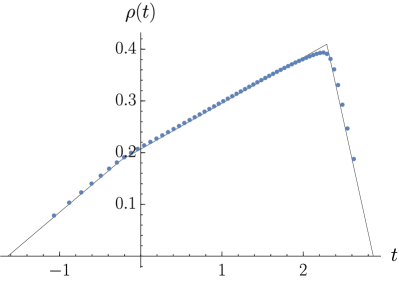
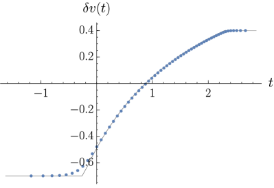
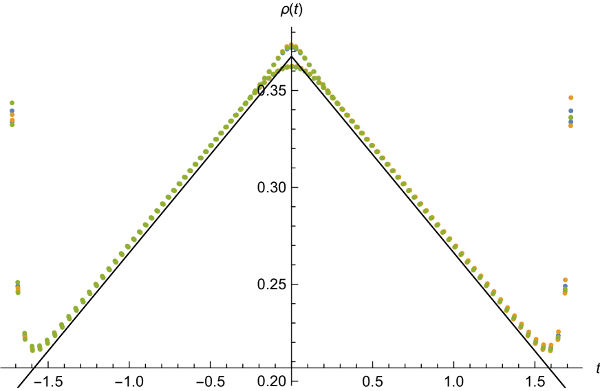
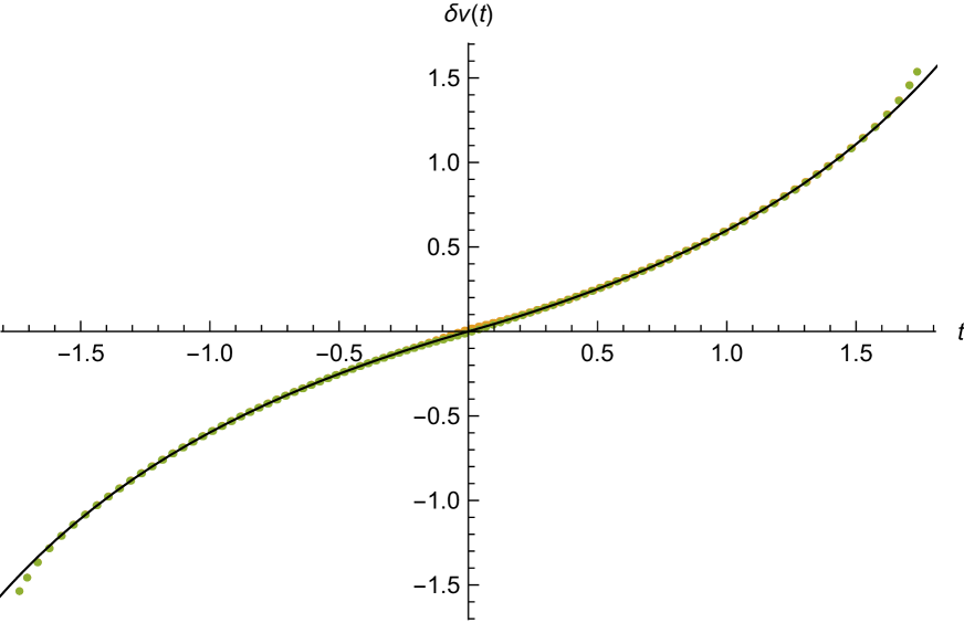
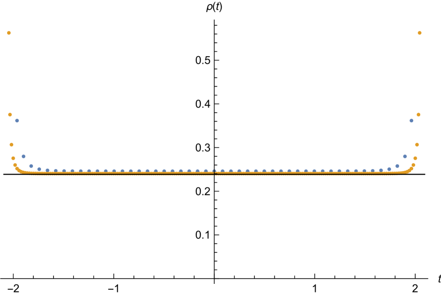
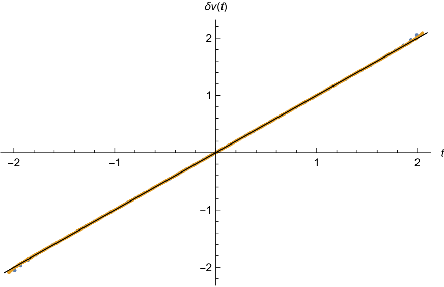
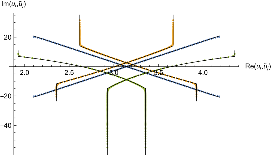
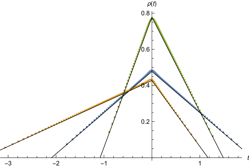
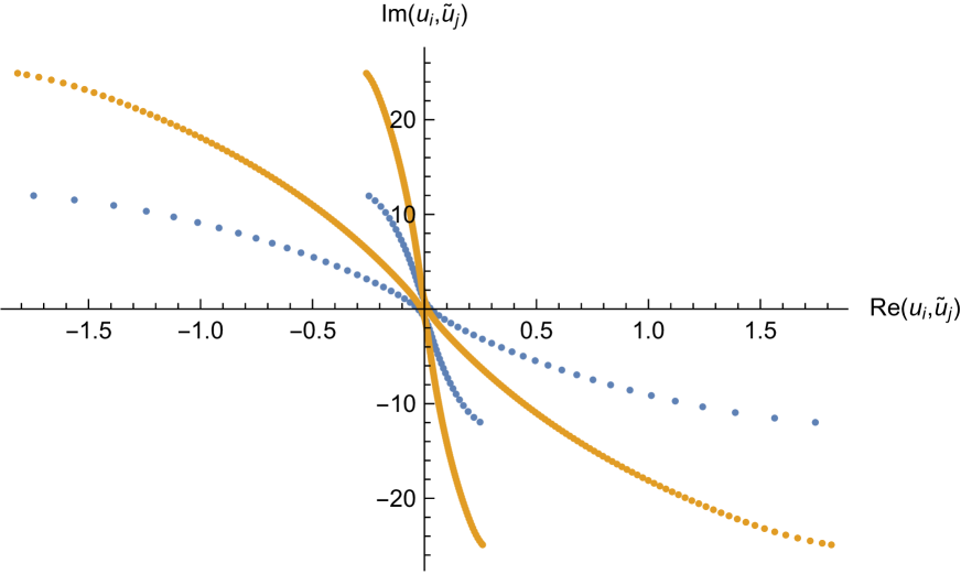
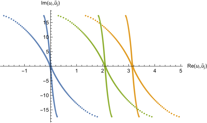
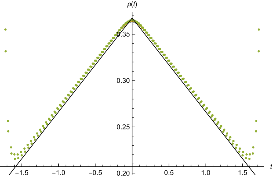
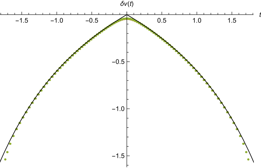
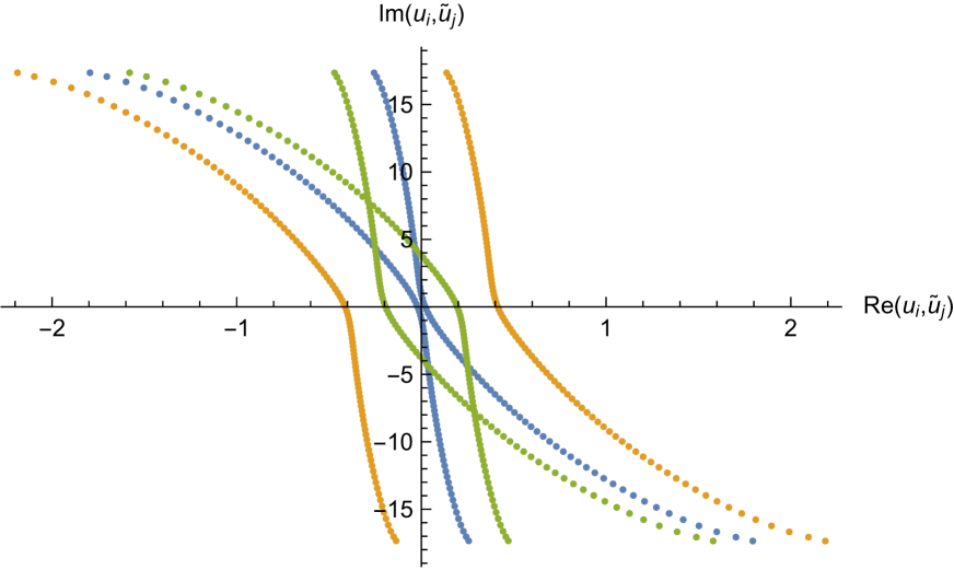
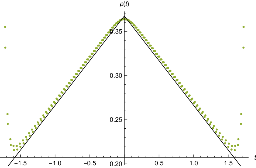
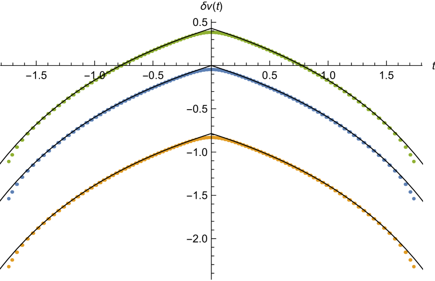
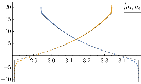
Let us quote some results from [20] where the numerical solution for the eigenvalues uisubscript𝑢𝑖u_{i} and u~isubscript~𝑢𝑖\tilde{u}_{i} for Δa={0.4,0.5,0.7,2π1.6}subscriptΔ𝑎0.40.50.72𝜋1.6\Delta_{a}=\{0.4,0.5,0.7,2\pi-1.6\} and N=60𝑁60N=60 is shown in Figure 1 quoted from [20]. The corresponding eigenvalue density ρ(t)𝜌𝑡\rho(t) and function δv(t)𝛿𝑣𝑡\delta v(t) are shown in Figure 2 quoted from [20].
Refer to caption
Figure 1: The solution to the BAE for Δa={0.4,0.5,0.7,2π1.6}subscriptΔ𝑎0.40.50.72𝜋1.6\Delta_{a}=\{0.4,0.5,0.7,2\pi-1.6\} and N=60𝑁60N=60. The solid lines correspond to the leading order expression obtained in [1].

Refer to captionRefer to caption

Figure 2: The eigenvalue density ρ(t)𝜌𝑡\rho(t) and the function δv(t)𝛿𝑣𝑡\delta v(t) for Δa={0.4,0.5,0.7,2π1.6}subscriptΔ𝑎0.40.50.72𝜋1.6\Delta_{a}=\{0.4,0.5,0.7,2\pi-1.6\} and N=60𝑁60N=60, compared with the leading order expression.

Once the eigenvalues are obtained, it is then simply a matter of numerically evaluating the index Eq. (2.28) on the solution to the BAE. For a given set of chemical potentials ΔasubscriptΔ𝑎\Delta_{a}, we compute logZ𝑍\log Z for a range of N𝑁N. We then subtract out the leading behavior Eq. (2.33) and decompose the residuals into a sum of four independent terms:

RelogZ=RelogZ0+A+B1𝔫1+B2𝔫2+B3𝔫3,Re𝑍Resubscript𝑍0𝐴subscript𝐵1subscript𝔫1subscript𝐵2subscript𝔫2subscript𝐵3subscript𝔫3{\rm Re}\log Z={\rm Re}\log Z_{0}+A+B_{1}\mathfrak{n}_{1}+B_{2}\mathfrak{n}_{2}+B_{3}\mathfrak{n}_{3}, (2.35)

where we have used the condition a𝔫a=2subscript𝑎subscript𝔫𝑎2\sum_{a}\mathfrak{n}_{a}=2. At this stage, we then perform a linear least-squares fit of A𝐴A and Basubscript𝐵𝑎B_{a} to the function

f(N)=f1N1/2+f2logN+f3+f4N1/2+f5N1+f6N3/2.𝑓𝑁subscript𝑓1superscript𝑁12subscript𝑓2𝑁subscript𝑓3subscript𝑓4superscript𝑁12subscript𝑓5superscript𝑁1subscript𝑓6superscript𝑁32f(N)=f_{1}N^{1/2}+f_{2}\log N+f_{3}+f_{4}N^{-1/2}+f_{5}N^{-1}+f_{6}N^{-3/2}. (2.36)

The results of the numerical fit are presented in Table 1 quoted from [20] whose main result is that the numerical evidence points to the coefficient of the logN𝑁\log N term being exactly 1/212-1/2. We thus have

RelogZ=N3/232Δ1Δ2Δ3Δ4a𝔫aΔa+N1/2f1(Δa,𝔫a)12logN+f3(Δa,𝔫a)+𝒪(N1/2),Re𝑍superscript𝑁3232subscriptΔ1subscriptΔ2subscriptΔ3subscriptΔ4subscript𝑎subscript𝔫𝑎subscriptΔ𝑎superscript𝑁12subscript𝑓1subscriptΔ𝑎subscript𝔫𝑎12𝑁subscript𝑓3subscriptΔ𝑎subscript𝔫𝑎𝒪superscript𝑁12{\rm Re}\log Z=-\frac{N^{3/2}}{3}\sqrt{2\Delta_{1}\Delta_{2}\Delta_{3}\Delta_{4}}\sum\limits_{a}\frac{\mathfrak{n}_{a}}{\Delta_{a}}+N^{1/2}f_{1}(\Delta_{a},\mathfrak{n}_{a})-\frac{1}{2}\log N+f_{3}(\Delta_{a},\mathfrak{n}_{a})+\mathcal{O}(N^{-1/2}), (2.37)

where f1subscript𝑓1f_{1} and f3subscript𝑓3f_{3} remain to be determined.

Δ1subscriptΔ1\Delta_{1} Δ2subscriptΔ2\Delta_{2} Δ3subscriptΔ3\Delta_{3} f1subscript𝑓1f_{1} f2subscript𝑓2f_{2} f3subscript𝑓3f_{3}
π/2𝜋2\pi/2 π/2𝜋2\pi/2 π/2𝜋2\pi/2 +3.05453.0545+3.0545 0.49990.4999-0.4999 3.04663.0466-3.0466
π/4𝜋4\pi/4 π/2𝜋2\pi/2 π/4𝜋4\pi/4
+4.22150.0491𝔫14.22150.0491subscript𝔫1+4.2215-0.0491\mathfrak{n}_{1}
0.1473𝔫20.0491𝔫30.1473subscript𝔫20.0491subscript𝔫3-0.1473\mathfrak{n}_{2}-0.0491\mathfrak{n}_{3}
0.4996+0.0000𝔫10.49960.0000subscript𝔫1-0.4996+0.0000\mathfrak{n}_{1}
+0.0000𝔫2+0.0000𝔫30.0000subscript𝔫20.0000subscript𝔫3+0.0000\mathfrak{n}_{2}+0.0000\mathfrak{n}_{3}
4.17100.2943𝔫14.17100.2943subscript𝔫1-4.1710-0.2943\mathfrak{n}_{1}
+0.0645𝔫20.2943𝔫30.0645subscript𝔫20.2943subscript𝔫3+0.0645\mathfrak{n}_{2}-0.2943\mathfrak{n}_{3}
0.30.30.3 0.40.40.4 0.50.50.5
+7.98550.2597𝔫17.98550.2597subscript𝔫1+7.9855-0.2597\mathfrak{n}_{1}
0.5833𝔫20.6411𝔫30.5833subscript𝔫20.6411subscript𝔫3-0.5833\mathfrak{n}_{2}-0.6411\mathfrak{n}_{3}
0.49940.0061𝔫10.49940.0061subscript𝔫1-0.4994-0.0061\mathfrak{n}_{1}
0.0020𝔫20.0007𝔫30.0020subscript𝔫20.0007subscript𝔫3-0.0020\mathfrak{n}_{2}-0.0007\mathfrak{n}_{3}
9.84040.9312𝔫19.84040.9312subscript𝔫1-9.8404-0.9312\mathfrak{n}_{1}
0.0293𝔫2+0.3739𝔫30.0293subscript𝔫20.3739subscript𝔫3-0.0293\mathfrak{n}_{2}+0.3739\mathfrak{n}_{3}
0.40.40.4 0.50.50.5 0.70.70.7
+6.66960.1904𝔫16.66960.1904subscript𝔫1+6.6696-0.1904\mathfrak{n}_{1}
0.4166𝔫20.4915𝔫30.4166subscript𝔫20.4915subscript𝔫3-0.4166\mathfrak{n}_{2}-0.4915\mathfrak{n}_{3}
0.49860.0016𝔫10.49860.0016subscript𝔫1-0.4986-0.0016\mathfrak{n}_{1}
0.0008𝔫20.0001𝔫30.0008subscript𝔫20.0001subscript𝔫3-0.0008\mathfrak{n}_{2}-0.0001\mathfrak{n}_{3}
7.53130.6893𝔫17.53130.6893subscript𝔫1-7.5313-0.6893\mathfrak{n}_{1}
0.1581𝔫2+0.2767𝔫30.1581subscript𝔫20.2767subscript𝔫3-0.1581\mathfrak{n}_{2}+0.2767\mathfrak{n}_{3}
Table 1: (ABJM) Numerical fit for RelogZ=RelogZ0+f1N1/2+f2logN+f3+Re𝑍Resubscript𝑍0subscript𝑓1superscript𝑁12subscript𝑓2𝑁subscript𝑓3{\rm Re}\log Z={\rm Re}\log Z_{0}+f_{1}N^{1/2}+f_{2}\log N+f_{3}+\cdots. The values of N𝑁N used in the fit range from 505050 to Nmaxsubscript𝑁maxN_{\rm max} in steps of 101010 where Nmax=290,150,190,120subscript𝑁max290150190120N_{\rm max}=290,150,190,120 for the four cases, respectively. We made use of the fact that the index is independent of the magnetic fluxes when performing the fit for the special case (Δa={π/2,π/2,π/2,π/2}subscriptΔ𝑎𝜋2𝜋2𝜋2𝜋2\Delta_{a}=\{\pi/2,\pi/2,\pi/2,\pi/2\}).

3 The topologically twisted index of N0,1,0superscript𝑁010N^{0,1,0}

In this section we study the Chern-Simons matter theory whose holographic dual is described by M-theory on AdS4×N0,1,0/ksubscriptAdS4superscript𝑁010subscript𝑘{\rm AdS}_{4}\times N^{0,1,0}/\mathbb{Z}_{k} [35, 36, 37]. The space N0,1,0superscript𝑁010N^{0,1,0} is a homogeneous Sasaki-Einstein manifold of dimension seven and defined as the coset SU(3)/U(1)𝑆𝑈3𝑈1SU(3)/U(1). The manifold has the isometry SU(3)×SU(2)𝑆𝑈3𝑆𝑈2SU(3)\times SU(2); the latter SU(2)𝑆𝑈2SU(2) is identified with the R-symmetry.

The field theory was discussed in [38, 39, 40] and shown to be described by the following quiver diagram:

(3.1)

The superpotential is

W=Tr(A1ϕ2B2B2ϕ1A1A2ϕ2B1+B1ϕ1A2+k2ϕ12k2ϕ22+q~ϕ1q).𝑊Trsubscript𝐴1subscriptitalic-ϕ2subscript𝐵2subscript𝐵2subscriptitalic-ϕ1subscript𝐴1subscript𝐴2subscriptitalic-ϕ2subscript𝐵1subscript𝐵1subscriptitalic-ϕ1subscript𝐴2𝑘2superscriptsubscriptitalic-ϕ12𝑘2superscriptsubscriptitalic-ϕ22~𝑞subscriptitalic-ϕ1𝑞\displaystyle W={\rm Tr}\left(A_{1}\phi_{2}B_{2}-B_{2}\phi_{1}A_{1}-A_{2}\phi_{2}B_{1}+B_{1}\phi_{1}A_{2}+\frac{k}{2}\phi_{1}^{2}-\frac{k}{2}\phi_{2}^{2}+\tilde{q}\phi_{1}q\right)\,. (3.2)

The free energy on S3superscript𝑆3S^{3} has been shown to match the gravity computation [38]; a discussion of the superconformal index was presented in [39, 40]. In the context of the topologically twisted index, this theory was recently considered by Hosseini and Mekareeya in [26] from which we borrow much, including the notation and the leading order analysis.

3.1 Numerical solutions to the system of BAEs

The topologically twisted index can be algorithmically assembled from the field theory content and the result is

Z𝑍\displaystyle Z =\displaystyle= 1(N!)2𝔪,𝔪~N𝒞i=1Ndxi2πixidx~i2πix~ixik𝔪ix~ik𝔪~i×ijN(1xixj)(1x~ix~j)1superscript𝑁2subscript𝔪~𝔪superscript𝑁subscript𝒞superscriptsubscriptproduct𝑖1𝑁𝑑subscript𝑥𝑖2𝜋𝑖subscript𝑥𝑖𝑑subscript~𝑥𝑖2𝜋𝑖subscript~𝑥𝑖superscriptsubscript𝑥𝑖𝑘subscript𝔪𝑖superscriptsubscript~𝑥𝑖𝑘subscript~𝔪𝑖superscriptsubscriptproduct𝑖𝑗𝑁1subscript𝑥𝑖subscript𝑥𝑗1subscript~𝑥𝑖subscript~𝑥𝑗\displaystyle\frac{1}{(N!)^{2}}\sum\limits_{\mathfrak{m},\tilde{\mathfrak{m}}\in\mathbb{Z}^{N}}\int_{\cal C}\prod\limits_{i=1}^{N}\frac{dx_{i}}{2\pi ix_{i}}\frac{d\tilde{x}_{i}}{2\pi i\tilde{x}_{i}}x_{i}^{k\mathfrak{m}_{i}}\tilde{x}_{i}^{-k\tilde{\mathfrak{m}}_{i}}\times\prod\limits_{i\neq j}^{N}\left(1-\frac{x_{i}}{x_{j}}\right)\left(1-\frac{\tilde{x}_{i}}{\tilde{x}_{j}}\right) (3.3)
×i,j=1Na=1,2(xix~jya1xix~jya)𝔪i𝔪~j𝔫a+1b=3,4(x~jxiyb1x~jxiyb)𝔪~j𝔪i𝔫b+1\displaystyle\times\prod\limits_{i,j=1}^{N}\prod\limits_{a=1,2}\left(\frac{\sqrt{\frac{x_{i}}{\tilde{x}_{j}}y_{a}}}{1-\frac{x_{i}}{\tilde{x}_{j}}y_{a}}\right)^{\mathfrak{m}_{i}-\tilde{\mathfrak{m}}_{j}-\mathfrak{n}_{a}+1}\prod\limits_{b=3,4}\left(\frac{\sqrt{\frac{\tilde{x}_{j}}{x_{i}}y_{b}}}{1-\frac{\tilde{x}_{j}}{x_{i}}y_{b}}\right)^{\tilde{\mathfrak{m}}_{j}-\mathfrak{m}_{i}-\mathfrak{n}_{b}+1}
×i=1N(xiyq1xiyq)r(𝔪i𝔫q+1)(1xiyq~11xiyq~)r(𝔪i𝔫q~+1).\displaystyle\times\prod\limits_{i=1}^{N}\Bigg{(}\frac{\sqrt{x_{i}y_{q}}}{1-x_{i}y_{q}}\Bigg{)}^{r(\mathfrak{m}_{i}-\mathfrak{n}_{q}+1)}\Bigg{(}\frac{\sqrt{\frac{1}{x_{i}}y_{\tilde{q}}}}{1-\frac{1}{x_{i}}y_{\tilde{q}}}\Bigg{)}^{r(-\mathfrak{m}_{i}-\mathfrak{n}_{\tilde{q}}+1)}.

Performing the summation over magnetic fluxes by introducing a large cut-off M𝑀M we get

Z𝑍\displaystyle Z =\displaystyle= 1(N!)2𝒞i=1Ndxi2πixidx~i2πix~iijN(1xixj)(1x~ix~j)1superscript𝑁2subscript𝒞superscriptsubscriptproduct𝑖1𝑁𝑑subscript𝑥𝑖2𝜋𝑖subscript𝑥𝑖𝑑subscript~𝑥𝑖2𝜋𝑖subscript~𝑥𝑖superscriptsubscriptproduct𝑖𝑗𝑁1subscript𝑥𝑖subscript𝑥𝑗1subscript~𝑥𝑖subscript~𝑥𝑗\displaystyle\frac{1}{(N!)^{2}}\int_{\cal C}\prod\limits_{i=1}^{N}\frac{dx_{i}}{2\pi ix_{i}}\frac{d\tilde{x}_{i}}{2\pi i\tilde{x}_{i}}\prod\limits_{i\neq j}^{N}\left(1-\frac{x_{i}}{x_{j}}\right)\left(1-\frac{\tilde{x}_{i}}{\tilde{x}_{j}}\right) (3.4)
×i,j=1Na=1,2(xix~jya1xix~jya)1𝔫ab=3,4(x~jxiyb1x~jxiyb)1𝔫b\displaystyle\times\prod\limits_{i,j=1}^{N}\prod\limits_{a=1,2}\left(\frac{\sqrt{\frac{x_{i}}{\tilde{x}_{j}}y_{a}}}{1-\frac{x_{i}}{\tilde{x}_{j}}y_{a}}\right)^{1-\mathfrak{n}_{a}}\prod\limits_{b=3,4}\left(\frac{\sqrt{\frac{\tilde{x}_{j}}{x_{i}}y_{b}}}{1-\frac{\tilde{x}_{j}}{x_{i}}y_{b}}\right)^{1-\mathfrak{n}_{b}}
×i=1N(xiyq1xiyq)r(1𝔫q)(1xiyq~11xiyq~)r(1𝔫q~)×i=1N(eiBi)MeiBi1j=1N(eiB~j)MeiB~j1,\displaystyle\times\prod\limits_{i=1}^{N}\Bigg{(}\frac{\sqrt{x_{i}y_{q}}}{1-x_{i}y_{q}}\Bigg{)}^{r(1-\mathfrak{n}_{q})}\Bigg{(}\frac{\sqrt{\frac{1}{x_{i}}y_{\tilde{q}}}}{1-\frac{1}{x_{i}}y_{\tilde{q}}}\Bigg{)}^{r(1-\mathfrak{n}_{\tilde{q}})}\times\prod\limits_{i=1}^{N}\frac{\big{(}e^{iB_{i}}\big{)}^{M}}{e^{iB_{i}}-1}\prod\limits_{j=1}^{N}\frac{\big{(}e^{i\tilde{B}_{j}}\big{)}^{M}}{e^{i\tilde{B}_{j}}-1},

where the Bethe Ansatz equations are

11\displaystyle 1 =\displaystyle= eiBi=xikj=1N(1y3x~jxi)(1y4x~jxi)(1y11x~jxi)(1y21x~jxi)×(xiyq1xiyq)r(1xiyq~11xiyq~)r,superscript𝑒𝑖subscript𝐵𝑖superscriptsubscript𝑥𝑖𝑘superscriptsubscriptproduct𝑗1𝑁1subscript𝑦3subscript~𝑥𝑗subscript𝑥𝑖1subscript𝑦4subscript~𝑥𝑗subscript𝑥𝑖1superscriptsubscript𝑦11subscript~𝑥𝑗subscript𝑥𝑖1superscriptsubscript𝑦21subscript~𝑥𝑗subscript𝑥𝑖superscriptsubscript𝑥𝑖subscript𝑦𝑞1subscript𝑥𝑖subscript𝑦𝑞𝑟superscript1subscript𝑥𝑖subscript𝑦~𝑞11subscript𝑥𝑖subscript𝑦~𝑞𝑟\displaystyle e^{iB_{i}}=x_{i}^{k}\prod\limits_{j=1}^{N}\frac{\left(1-y_{3}\frac{\tilde{x}_{j}}{x_{i}}\right)\left(1-y_{4}\frac{\tilde{x}_{j}}{x_{i}}\right)}{\left(1-y_{1}^{-1}\frac{\tilde{x}_{j}}{x_{i}}\right)\left(1-y_{2}^{-1}\frac{\tilde{x}_{j}}{x_{i}}\right)}\times\Bigg{(}\frac{\sqrt{x_{i}y_{q}}}{1-x_{i}y_{q}}\Bigg{)}^{r}\Bigg{(}\frac{\sqrt{\frac{1}{x_{i}}y_{\tilde{q}}}}{1-\frac{1}{x_{i}}y_{\tilde{q}}}\Bigg{)}^{-r},
11\displaystyle 1 =\displaystyle= eiB~j=x~jki=1N(1y3x~jxi)(1y4x~jxi)(1y11x~jxi)(1y21x~jxi).superscript𝑒𝑖subscript~𝐵𝑗superscriptsubscript~𝑥𝑗𝑘superscriptsubscriptproduct𝑖1𝑁1subscript𝑦3subscript~𝑥𝑗subscript𝑥𝑖1subscript𝑦4subscript~𝑥𝑗subscript𝑥𝑖1superscriptsubscript𝑦11subscript~𝑥𝑗subscript𝑥𝑖1superscriptsubscript𝑦21subscript~𝑥𝑗subscript𝑥𝑖\displaystyle e^{i\tilde{B}_{j}}=\tilde{x}_{j}^{k}\prod\limits_{i=1}^{N}\frac{\left(1-y_{3}\frac{\tilde{x}_{j}}{x_{i}}\right)\left(1-y_{4}\frac{\tilde{x}_{j}}{x_{i}}\right)}{\left(1-y_{1}^{-1}\frac{\tilde{x}_{j}}{x_{i}}\right)\left(1-y_{2}^{-1}\frac{\tilde{x}_{j}}{x_{i}}\right)}. (3.5)

The compact expression for the index in terms of solutions to the Bethe-Ansatz equations Eq. (3.1) takes the form

Z(ya,𝔫a)𝑍subscript𝑦𝑎subscript𝔫𝑎\displaystyle Z\left(y_{a},\mathfrak{n}_{a}\right) =\displaystyle= (1)Nr2yq12Nr𝔫qyq~12Nr𝔫q~a=14ya12N2𝔫asuperscript1𝑁𝑟2superscriptsubscript𝑦𝑞12𝑁𝑟subscript𝔫𝑞superscriptsubscript𝑦~𝑞12𝑁𝑟subscript𝔫~𝑞superscriptsubscriptproduct𝑎14superscriptsubscript𝑦𝑎12superscript𝑁2subscript𝔫𝑎\displaystyle\left(-1\right)^{\frac{Nr}{2}}y_{q}^{-\frac{1}{2}Nr\mathfrak{n}_{q}}y_{\tilde{q}}^{-\frac{1}{2}Nr\mathfrak{n}_{\tilde{q}}}\prod_{a=1}^{4}y_{a}^{-\frac{1}{2}N^{2}\mathfrak{n}_{a}} (3.6)
×IBAE[1det𝔹i=1NxiNx~iNij(1xixj)(1x~ix~j)i,j=1Na=1,2(x~jyaxi)1𝔫aa=3,4(xiyax~j)1𝔫a\displaystyle\times\sum_{I\in BAE}\left[\frac{1}{\det\mathbb{B}}\frac{\prod_{i=1}^{N}x_{i}^{N}\tilde{x}_{i}^{N}\prod_{i\neq j}\left(1-\frac{x_{i}}{x_{j}}\right)\left(1-\frac{\tilde{x}_{i}}{\tilde{x}_{j}}\right)}{\prod_{i,j=1}^{N}\prod_{a=1,2}\left(\tilde{x}_{j}-y_{a}x_{i}\right)^{1-\mathfrak{n}_{a}}\prod_{a=3,4}\left(x_{i}-y_{a}\tilde{x}_{j}\right)^{1-\mathfrak{n}_{a}}}\right.
×i=1Nxi12r(1xiyq)r(1𝔫q)(xiyq~)r(1𝔫q~)].\displaystyle\left.\times\prod_{i=1}^{N}\frac{x_{i}^{\frac{1}{2}r}}{\left(1-x_{i}y_{q}\right)^{r\left(1-\mathfrak{n}_{q}\right)}\left(x_{i}-y_{\tilde{q}}\right)^{r\left(1-\mathfrak{n}_{\tilde{q}}\right)}}\right].

The transformation matrix 𝔹𝔹\mathbb{B} describing the change in integration variables from xisubscript𝑥𝑖x_{i} to Bisubscript𝐵𝑖B_{i} is

𝔹|BAEs=(δjl[km=1NGjm+rxj(1xjyq~1xjyq1)]GjlGljδjl[k+m=1NGmj]),evaluated-at𝔹BAEssubscript𝛿𝑗𝑙delimited-[]𝑘superscriptsubscript𝑚1𝑁subscript𝐺𝑗𝑚𝑟subscript𝑥𝑗1subscript𝑥𝑗subscript𝑦~𝑞1subscript𝑥𝑗superscriptsubscript𝑦𝑞1subscript𝐺𝑗𝑙subscript𝐺𝑙𝑗subscript𝛿𝑗𝑙delimited-[]𝑘superscriptsubscript𝑚1𝑁subscript𝐺𝑚𝑗\mathbb{B}\Big{|}_{\rm BAEs}=\left(\begin{array}[]{cc}\delta_{jl}\left[k-\sum_{m=1}^{N}G_{jm}+rx_{j}\left(\frac{1}{x_{j}-y_{\tilde{q}}}-\frac{1}{x_{j}-y_{q}^{-1}}\right)\right]&G_{jl}\\ -G_{lj}&\delta_{jl}\left[k+\sum_{m=1}^{N}G_{mj}\right]\end{array}\right), (3.7)

where

D(z)=(1zy3)(1zy4)(1zy11)(1zy21),Gij=logD(z)logz|z=x~j/xi.formulae-sequence𝐷𝑧1𝑧subscript𝑦31𝑧subscript𝑦41𝑧superscriptsubscript𝑦111𝑧superscriptsubscript𝑦21subscript𝐺𝑖𝑗evaluated-at𝐷𝑧𝑧𝑧subscript~𝑥𝑗subscript𝑥𝑖D(z)=\frac{(1-zy_{3})(1-zy_{4})}{(1-zy_{1}^{-1})(1-zy_{2}^{-1})},\qquad G_{ij}=\frac{\partial\log D(z)}{\partial\log z}\Big{|}_{z=\tilde{x}_{j}/x_{i}}. (3.8)

The Bethe-Ansatz equations Eq. (3.1) can be obtained from the potential which takes the form

𝒱𝒱\displaystyle\mathcal{V} =\displaystyle= i=1N[k2(u~i2ui2)2π(n~iu~iniui)]superscriptsubscript𝑖1𝑁delimited-[]𝑘2superscriptsubscript~𝑢𝑖2superscriptsubscript𝑢𝑖22𝜋subscript~𝑛𝑖subscript~𝑢𝑖subscript𝑛𝑖subscript𝑢𝑖\displaystyle\sum\limits_{i=1}^{N}\left[\frac{k}{2}\left(\tilde{u}_{i}^{2}-u_{i}^{2}\right)-2\pi\left(\tilde{n}_{i}\tilde{u}_{i}-n_{i}u_{i}\right)\right] (3.9)
+i,j=1N[a=3,4Li2(ei(u~jui+Δa))a=1,2Li2(ei(u~juiΔa))]superscriptsubscript𝑖𝑗1𝑁delimited-[]subscript𝑎34subscriptLi2superscript𝑒𝑖subscript~𝑢𝑗subscript𝑢𝑖subscriptΔ𝑎subscript𝑎12subscriptLi2superscript𝑒𝑖subscript~𝑢𝑗subscript𝑢𝑖subscriptΔ𝑎\displaystyle+\sum\limits_{i,j=1}^{N}\left[\sum\limits_{a=3,4}{\rm Li}_{2}\left(e^{i\left(\tilde{u}_{j}-u_{i}+\Delta_{a}\right)}\right)-\sum\limits_{a=1,2}{\rm Li}_{2}\left(e^{i\left(\tilde{u}_{j}-u_{i}-\Delta_{a}\right)}\right)\right]
+ri=1N[Li2(ei(ui+Δq~))Li2(ei(uiΔq))]+r2i=1N[(Δq~+Δq2π)ui],𝑟superscriptsubscript𝑖1𝑁delimited-[]subscriptLi2superscript𝑒𝑖subscript𝑢𝑖subscriptΔ~𝑞subscriptLi2superscript𝑒𝑖subscript𝑢𝑖subscriptΔ𝑞𝑟2superscriptsubscript𝑖1𝑁delimited-[]subscriptΔ~𝑞subscriptΔ𝑞2𝜋subscript𝑢𝑖\displaystyle+r\sum\limits_{i=1}^{N}\left[{\rm Li}_{2}\left(e^{i\left(-u_{i}+\Delta_{\tilde{q}}\right)}\right)-{\rm Li}_{2}\left(e^{i\left(-u_{i}-\Delta_{q}\right)}\right)\right]+\frac{r}{2}\sum\limits_{i=1}^{N}\left[\left(\Delta_{\tilde{q}}+\Delta_{q}-2\pi\right)u_{i}\right],

where

i=1N[2π(n~iu~iniui)]=(4πa=14Δa)i>jN(u~jui)=2πi>jN(u~jui).superscriptsubscript𝑖1𝑁delimited-[]2𝜋subscript~𝑛𝑖subscript~𝑢𝑖subscript𝑛𝑖subscript𝑢𝑖4𝜋superscriptsubscript𝑎14subscriptΔ𝑎superscriptsubscript𝑖𝑗𝑁subscript~𝑢𝑗subscript𝑢𝑖2𝜋superscriptsubscript𝑖𝑗𝑁subscript~𝑢𝑗subscript𝑢𝑖\sum\limits_{i=1}^{N}\left[-2\pi\left(\tilde{n}_{i}\tilde{u}_{i}-n_{i}u_{i}\right)\right]=\left(4\pi-\sum\limits_{a=1}^{4}\Delta_{a}\right)\sum\limits_{i>j}^{N}\left(\tilde{u}_{j}-u_{i}\right)=2\pi\sum\limits_{i>j}^{N}\left(\tilde{u}_{j}-u_{i}\right). (3.10)

We use the leading order solution to the system of BAEs in [26] as a seed for the exact numerical solution to the BAE’s in Eq. (3.1). We will assume, as in [25], that 0<v(t)+Δq<2π0𝑣𝑡subscriptΔ𝑞2𝜋0<v(t)+\Delta_{q}<2\pi and 0<v(t)+Δq~<2π0𝑣𝑡subscriptΔ~𝑞2𝜋0<-v(t)+\Delta_{\tilde{q}}<2\pi, then we have

Δq<v(t)<Δq~,subscriptΔ𝑞𝑣𝑡subscriptΔ~𝑞-\Delta_{q}<v(t)<\Delta_{\tilde{q}}, (3.11)

thus we set the initial real part axis to be

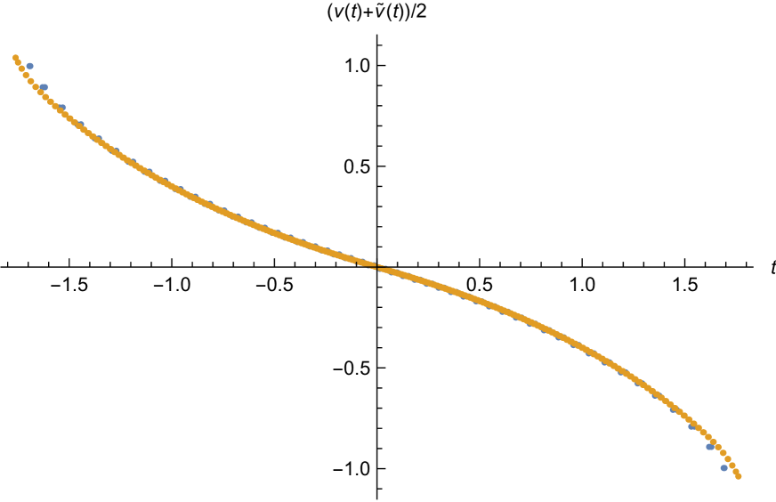
v(t)+v~(t)2=Δq~Δq2.𝑣𝑡~𝑣𝑡2subscriptΔ~𝑞subscriptΔ𝑞2\frac{v(t)+\tilde{v}(t)}{2}=\frac{\Delta_{\tilde{q}}-\Delta_{q}}{2}. (3.12)

The marginality condition on the superpotential requires that Δq+Δq~=πsubscriptΔ𝑞subscriptΔ~𝑞𝜋\Delta_{q}+\Delta_{\tilde{q}}=\pi. For comparison, recall that in the ABJM theory, the real part axis defined above is π𝜋\pi when k=1𝑘1k=1, thus we assume the range of the real part axis here should be near to π𝜋\pi to match with the ABJM theory when r=0𝑟0r=0. If we set (Δq~Δq)/2=πsubscriptΔ~𝑞subscriptΔ𝑞2𝜋\left(\Delta_{\tilde{q}}-\Delta_{q}\right)/2=\pi we will get {Δq,Δq~}={π/2,3π/2}subscriptΔ𝑞subscriptΔ~𝑞𝜋23𝜋2\{\Delta_{q},\Delta_{\tilde{q}}\}=\{-\pi/2,3\pi/2\}. We will see the effects of the values of {Δq,Δq~}subscriptΔ𝑞subscriptΔ~𝑞\{\Delta_{q},\Delta_{\tilde{q}}\} in the numerical solutions.

Before entering the details of the numerical analysis, let us remark that, as compared to ABJM, the system has three new parameters which are r𝑟r – the number of flavors of fundamental hypermultiplets, and the fugacities {Δq,Δq~}subscriptΔ𝑞subscriptΔ~𝑞\{\Delta_{q},\Delta_{\tilde{q}}\} discussed above. Our goal is to explore the space of new parameters as well as those parameters already present in ABJM, namely N𝑁N – the rank of the gauge group and Δa={Δ1,Δ2,Δ3,Δ4}subscriptΔ𝑎subscriptΔ1subscriptΔ2subscriptΔ3subscriptΔ4\Delta_{a}=\{\Delta_{1},\Delta_{2},\Delta_{3},\Delta_{4}\} – the fugacities of the bi-fundamental matter.

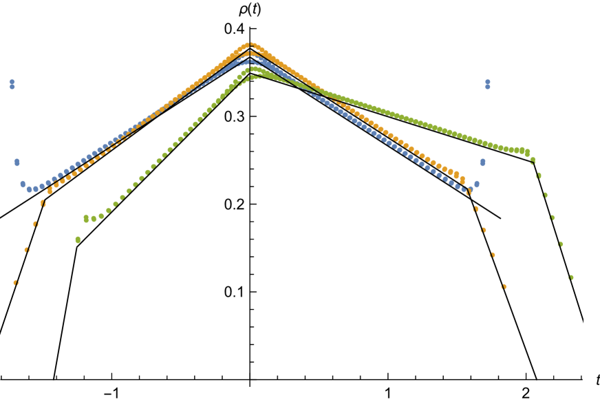
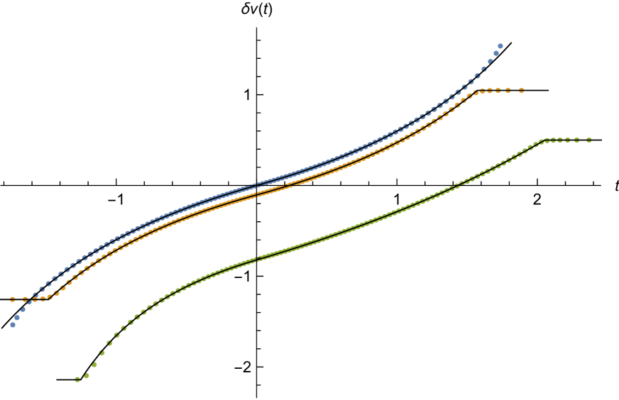
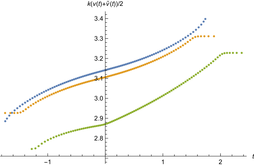
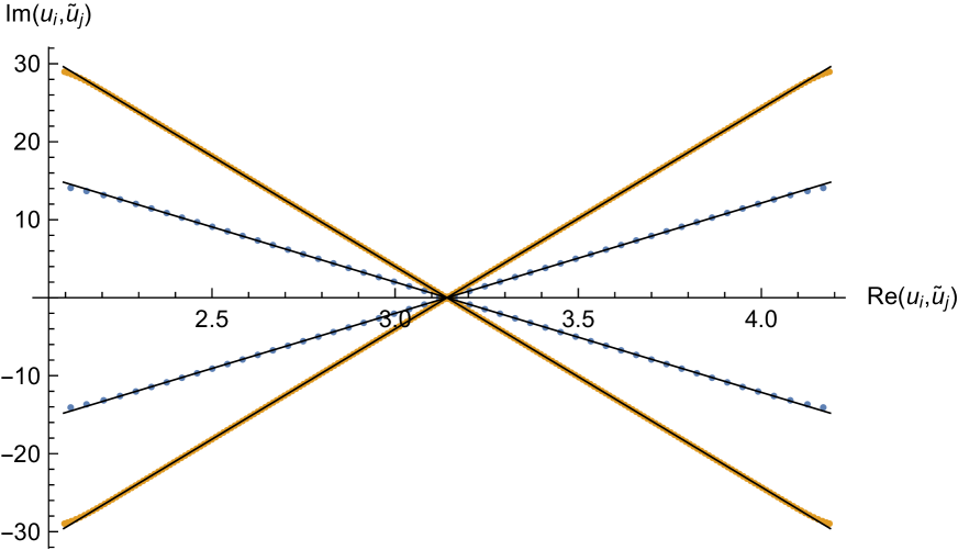
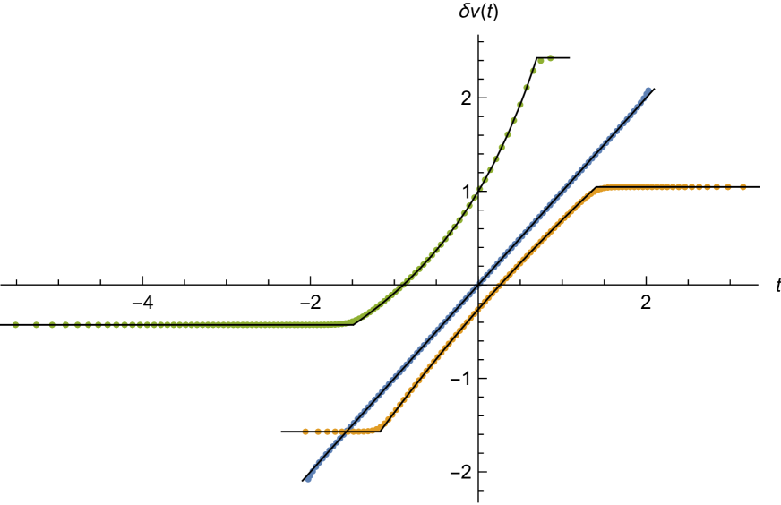
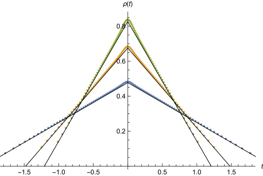
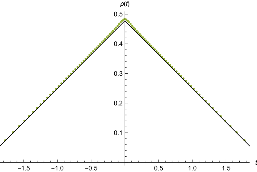
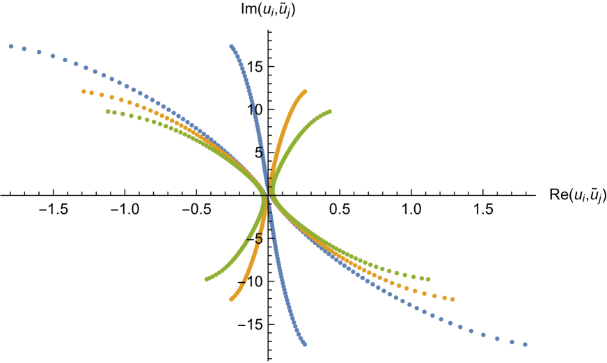
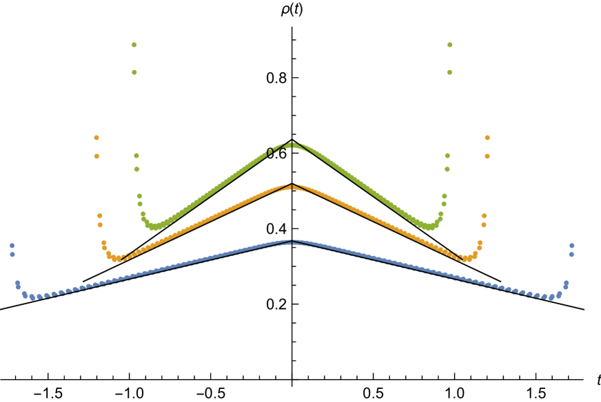
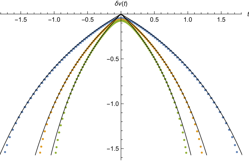
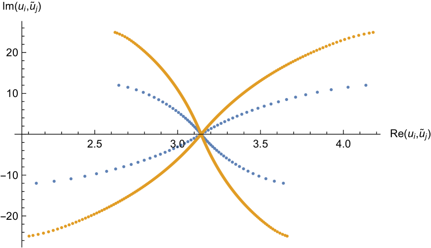
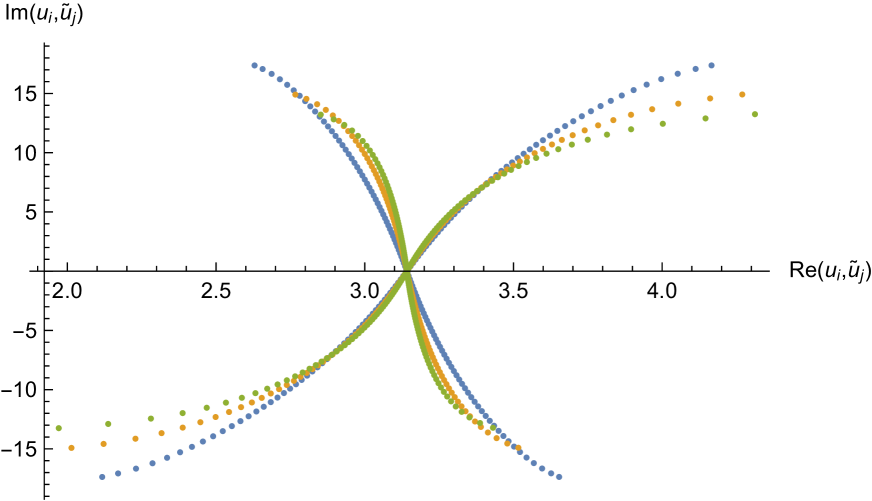
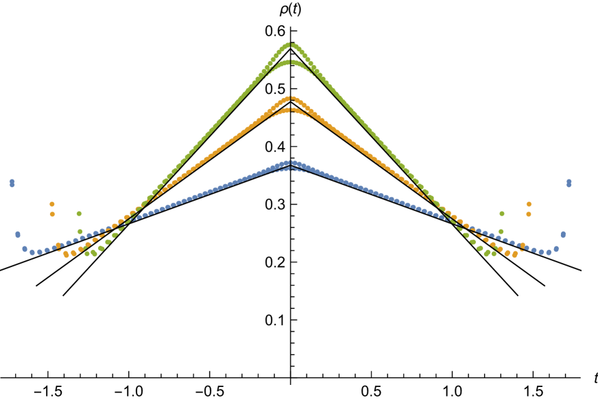
The numerical solutions to the BAEs can be obtained using FindRoot in Mathematica as implemented in[20, 41]. In the following we focus on the case k=1𝑘1k=1. The numerical solutions for different values of N𝑁N, r𝑟r, {Δq,Δq~}subscriptΔ𝑞subscriptΔ~𝑞\{\Delta_{q},\Delta_{\tilde{q}}\} and ΔasubscriptΔ𝑎\Delta_{a} are shown in Figures 4 - 10. The black lines are the analytical results in [26].

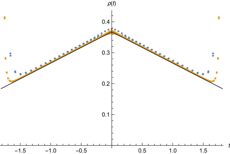
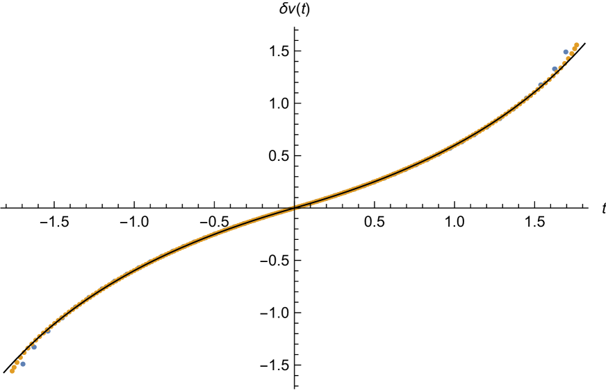
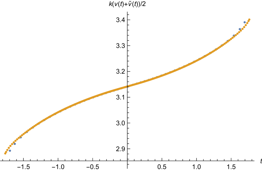
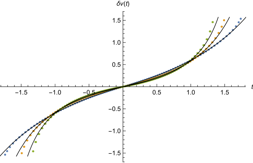
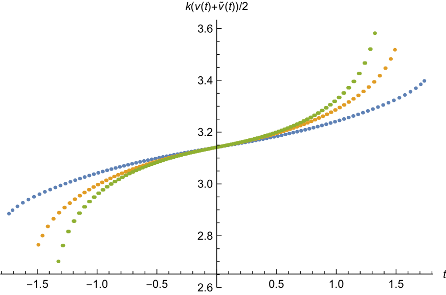
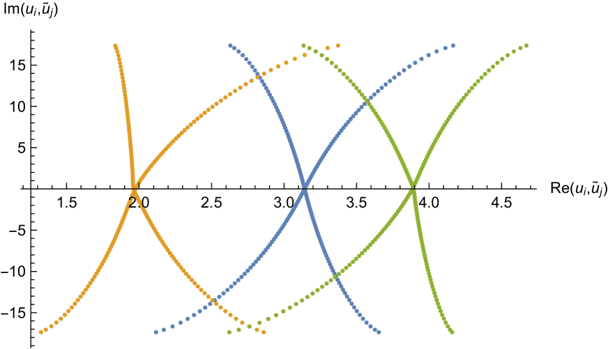
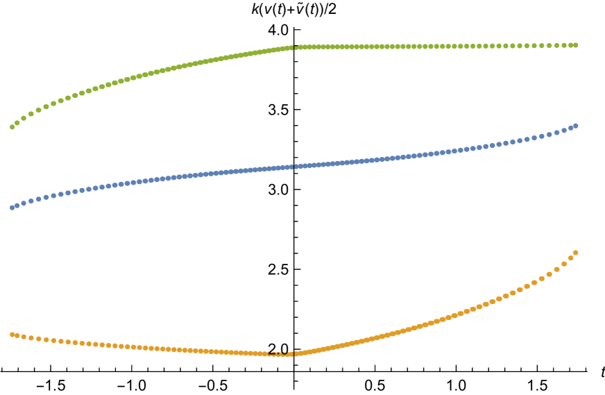
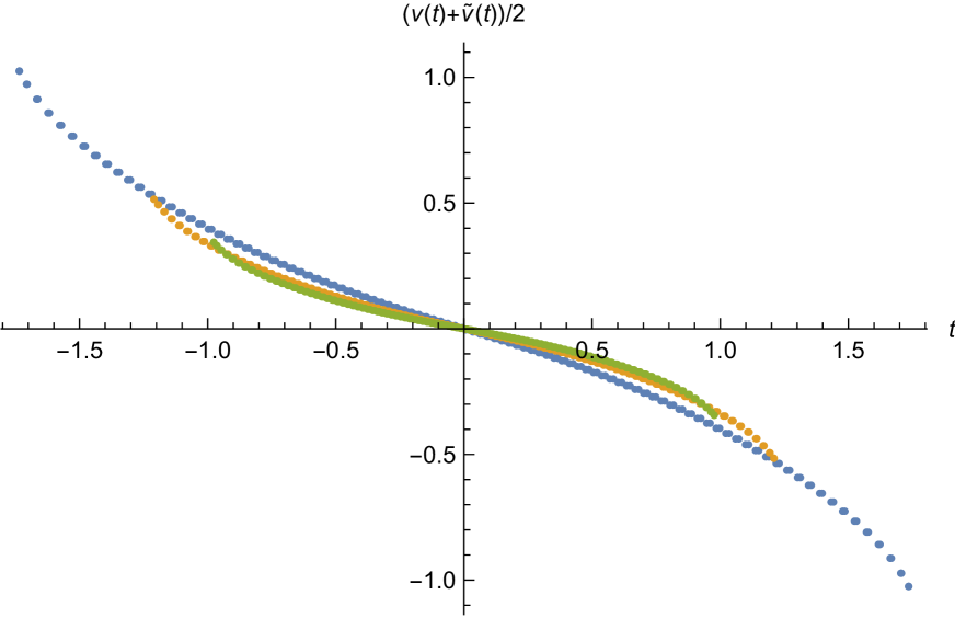
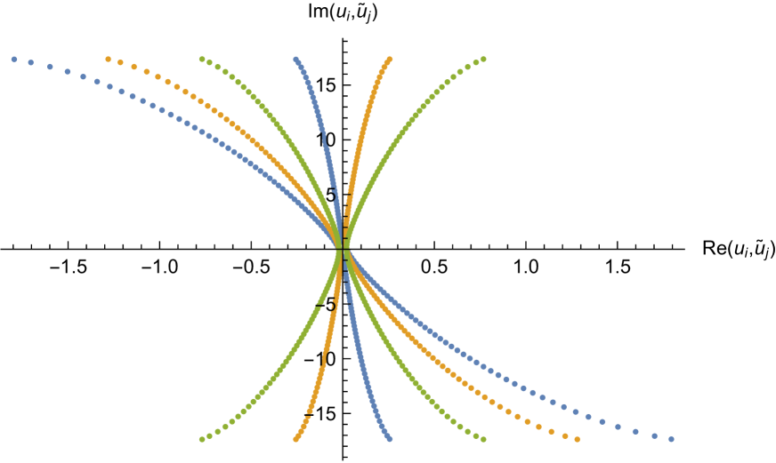
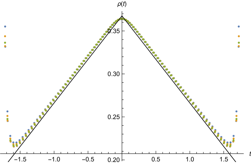
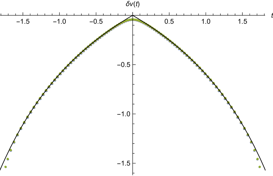
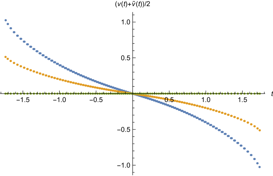
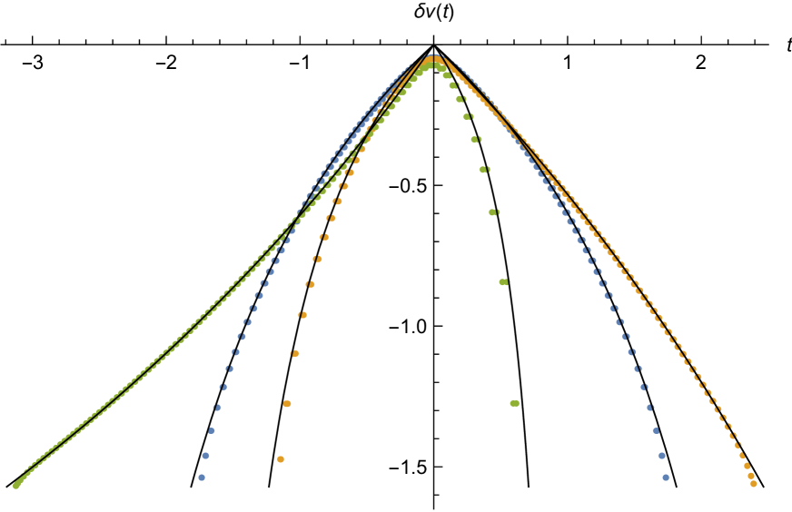
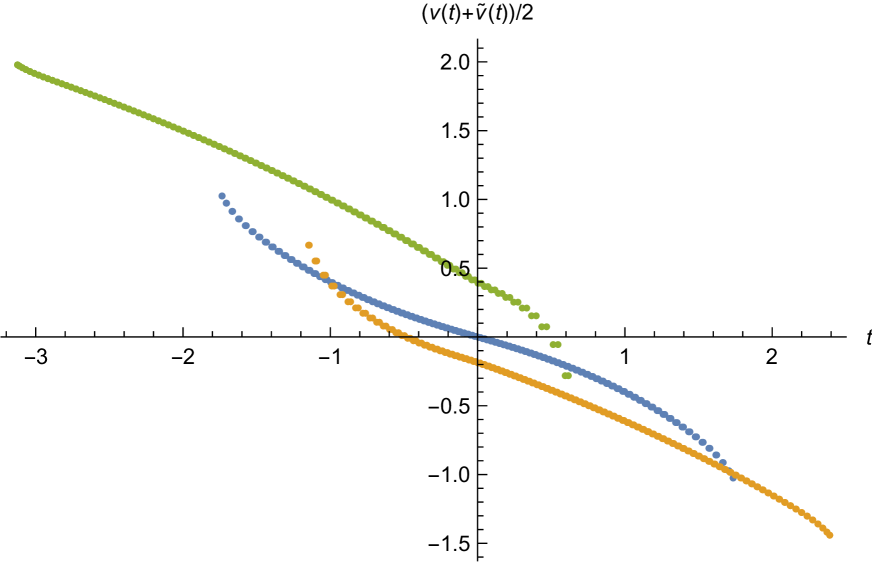
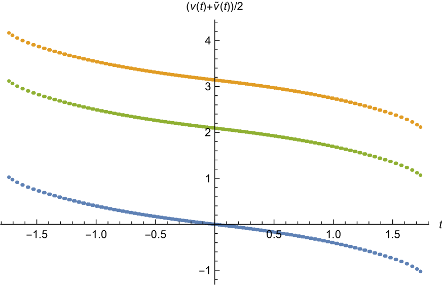
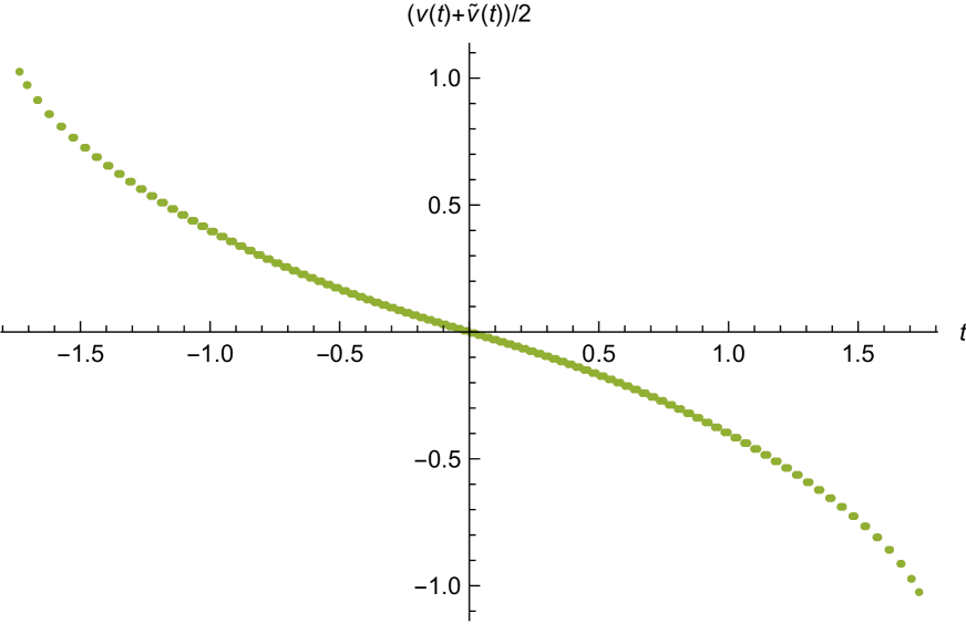
The numerical solutions show that the eigenvalues are not reflectively symmetric about π𝜋\pi alone the real axis as the ABJM theory. Furthermore, the imaginary part of uisubscript𝑢𝑖u_{i} is not exactly the same as u~isubscript~𝑢𝑖\tilde{u}_{i} so that there are two numerical results of the eigenvalue density ρ(t)𝜌𝑡\rho(t), the real part difference δv(t)𝛿𝑣𝑡\delta v(t) and the real part axis (v(t)+v~(t))/2𝑣𝑡~𝑣𝑡2\left(v(t)+\tilde{v}(t)\right)/2, though it is not obvious in the last two because of overlapping.
Refer to caption
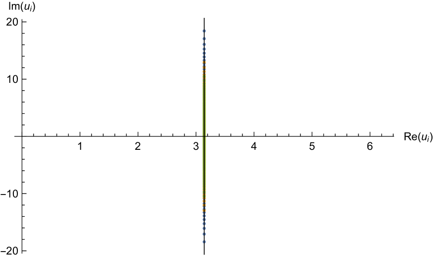
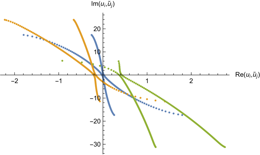
(a) Eigenvalue distribution
Refer to caption
(b) Eigenvalue density ρ(t)𝜌𝑡\rho(t)
Refer to caption
(c) Real part difference δv(t)𝛿𝑣𝑡\delta v(t)
Refer to caption
(d) Real part axis k(v(t)+v~(t))/2𝑘𝑣𝑡~𝑣𝑡2k(v(t)+\tilde{v}(t))/2
Refer to caption
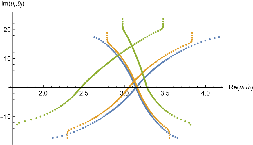
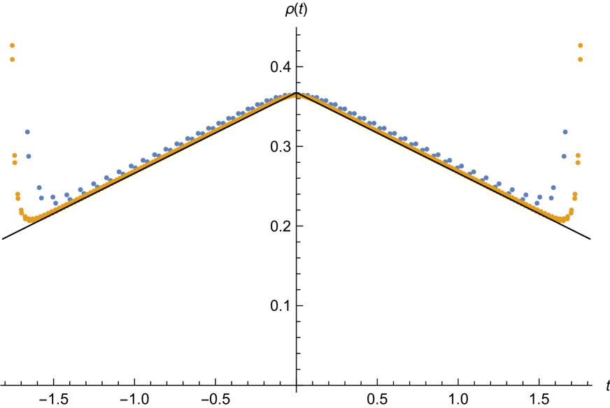
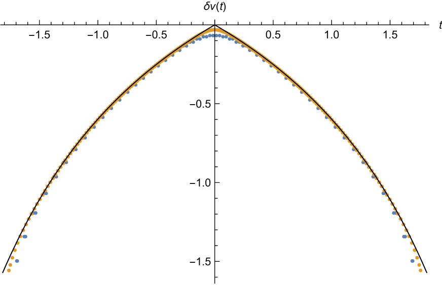
Figure 4: Eigenvalues for the special case Δa={π2,π2,π2,π2}subscriptΔ𝑎𝜋2𝜋2𝜋2𝜋2\Delta_{a}=\{\frac{\pi}{2},\frac{\pi}{2},\frac{\pi}{2},\frac{\pi}{2}\} for N=50𝑁50N=50 (blue) and 200200200 (orange) with the same other parameters.

In Figure 4 we describe the eigenvalues as exact numerical solutions of the BAE Eq. (3.1). The plots show that the imaginary part of the eigenvalues scales as N1/2superscript𝑁12N^{1/2}. The eigenvalue densities are very well described by the leading analytical result of [26] except for some deviations at the edges of the intervals.
Refer to caption
(a) Eigenvalue distribution
Refer to caption
(b) Eigenvalue density ρ(t)𝜌𝑡\rho(t)
Refer to caption
(c) Real part difference δv(t)𝛿𝑣𝑡\delta v(t)
Refer to caption
(d) Real part axis k(v(t)+v~(t))/2𝑘𝑣𝑡~𝑣𝑡2k(v(t)+\tilde{v}(t))/2
Refer to caption
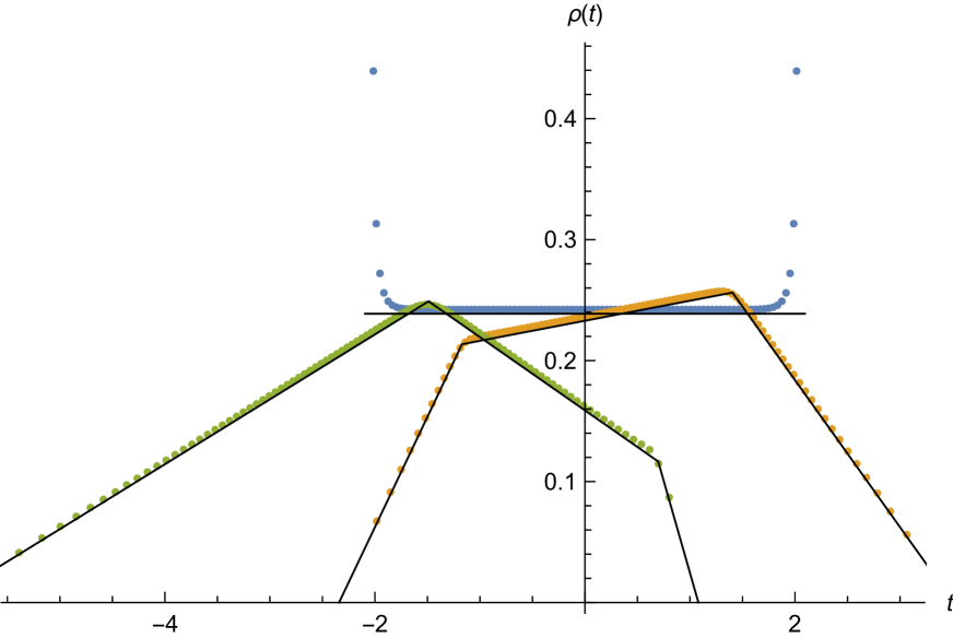
Figure 6: Eigenvalues for the special case Δa={π2,π2,π2,π2}subscriptΔ𝑎𝜋2𝜋2𝜋2𝜋2\Delta_{a}=\{\frac{\pi}{2},\frac{\pi}{2},\frac{\pi}{2},\frac{\pi}{2}\} for r=1𝑟1r=1 (blue), 222 (orange) and 333 (green) with other parameters kept the same.
Refer to caption
(a) Eigenvalue distribution
Refer to caption
(b) Eigenvalue density ρ(t)𝜌𝑡\rho(t)
Refer to caption
(c) Real part difference δv(t)𝛿𝑣𝑡\delta v(t)
Refer to caption
(d) Real part axis k(v(t)+v~(t))/2𝑘𝑣𝑡~𝑣𝑡2k(v(t)+\tilde{v}(t))/2
Refer to caption
Figure 8: Eigenvalues for the special case Δa={π2,π2,π2,π2}subscriptΔ𝑎𝜋2𝜋2𝜋2𝜋2\Delta_{a}=\{\frac{\pi}{2},\frac{\pi}{2},\frac{\pi}{2},\frac{\pi}{2}\} for {Δq,Δq~}={π2,3π2}subscriptΔ𝑞subscriptΔ~𝑞𝜋23𝜋2\{\Delta_{q},\Delta_{\tilde{q}}\}=\{-\frac{\pi}{2},\frac{3\pi}{2}\} (blue), {0,π}0𝜋\{0,\pi\} (orange) and {1π2,1+3π2}1𝜋213𝜋2\{-1-\frac{\pi}{2},1+\frac{3\pi}{2}\} (green) with the same other parameters.

Figure 6 explores the nature of the eigenvalues as one changes the number of fundamental flavors r𝑟r, the most prominent change is accurately captured by the slope in the eigenvalue density. In Figure 8 we explore the effects of changing the fugacities {Δq,Δq~}subscriptΔ𝑞subscriptΔ~𝑞\{\Delta_{q},\Delta_{\tilde{q}}\}. The main effect is in the real part axis (v(t)+v~(t))/2𝑣𝑡~𝑣𝑡2\left(v(t)+\tilde{v}(t)\right)/2.

Refer to caption
(a) Eigenvalue distribution
Refer to caption
(b) Eigenvalue density ρ(t)𝜌𝑡\rho(t)
Refer to caption
(c) Real part difference δv(t)𝛿𝑣𝑡\delta v(t)
Refer to caption
(d) Real part axis k(v(t)+v~(t))/2𝑘𝑣𝑡~𝑣𝑡2k(v(t)+\tilde{v}(t))/2
Refer to caption
Figure 10: Eigenvalues for the special case Δa={π2,π2,π2,π2}subscriptΔ𝑎𝜋2𝜋2𝜋2𝜋2\Delta_{a}=\{\frac{\pi}{2},\frac{\pi}{2},\frac{\pi}{2},\frac{\pi}{2}\} (blue), and the general cases Δa={π3,3π5,2π5,2π3}subscriptΔ𝑎𝜋33𝜋52𝜋52𝜋3\Delta_{a}=\{\frac{\pi}{3},\frac{3\pi}{5},\frac{2\pi}{5},\frac{2\pi}{3}\} (orange) and Δa={12,1,1+π,12+π}subscriptΔ𝑎1211𝜋12𝜋\Delta_{a}=\{\frac{1}{2},1,-1+\pi,-\frac{1}{2}+\pi\} (green) with the same other parameters.

Finally, in Figure 10 we explore the eigenvalues away from the symmetric point of the bi-fundamental fugacities. As in the ABJM case [20], this is numerically challenging as one needs confront numerically, various numerical singularities due to branch points in the polylogarithmic functions.

3.2 The subleading term of the index at large N𝑁N

Having achieved control of the eigenvalues we can proceed to analyze the index. As the ABJM theory, we expand the index beyond the leading order in N𝑁N and we expect the subleading behavior of the index to have the form

RelogZ=f1(k,r,Δ,𝔫)N3/2+f2(k,r,Δ,𝔫)N1/2+f3(k,r,Δ,𝔫)logN+f4(k,r,Δ,𝔫)+𝒪(N1/2),Re𝑍subscript𝑓1𝑘𝑟Δ𝔫superscript𝑁32subscript𝑓2𝑘𝑟Δ𝔫superscript𝑁12subscript𝑓3𝑘𝑟Δ𝔫𝑁subscript𝑓4𝑘𝑟Δ𝔫𝒪superscript𝑁12{\rm Re}\log Z=f_{1}(k,r,\Delta,\mathfrak{n})N^{3/2}+f_{2}(k,r,\Delta,\mathfrak{n})N^{1/2}+f_{3}(k,r,\Delta,\mathfrak{n})\log{N}+f_{4}(k,r,\Delta,\mathfrak{n})+\mathcal{O}(N^{-1/2}), (3.13)

where the functions f1subscript𝑓1f_{1}, f2subscript𝑓2f_{2}, f3subscript𝑓3f_{3} and f4subscript𝑓4f_{4} are linear in the magnetic fluxes 𝔫𝔫\mathfrak{n}.

For k=1𝑘1k=1 and a given set of ΔasubscriptΔ𝑎\Delta_{a}, r𝑟r and {Δq,Δq~}subscriptΔ𝑞subscriptΔ~𝑞\{\Delta_{q},\Delta_{\tilde{q}}\}, we can compute the index Eq. (3.6) and RelogZRe𝑍{\rm Re}\log Z for a range of N𝑁N using the numerical solutions obtained in section 3.1. Then we decompose RelogZRe𝑍{\rm Re}\log Z into a sum of four independent terms

RelogZ=A+B1𝔫3+B2𝔫4+B3𝔫q,Re𝑍𝐴subscript𝐵1subscript𝔫3subscript𝐵2subscript𝔫4subscript𝐵3subscript𝔫𝑞{\rm Re}\log Z=A+B_{1}\mathfrak{n}_{3}+B_{2}\mathfrak{n}_{4}+B_{3}\mathfrak{n}_{q}, (3.14)

where we have used the marginality condition on the superpotential 𝔫1+𝔫4=1subscript𝔫1subscript𝔫41\mathfrak{n}_{1}+\mathfrak{n}_{4}=1, 𝔫2+𝔫3=1subscript𝔫2subscript𝔫31\mathfrak{n}_{2}+\mathfrak{n}_{3}=1 and 𝔫q+𝔫q~=1subscript𝔫𝑞subscript𝔫~𝑞1\mathfrak{n}_{q}+\mathfrak{n}_{\tilde{q}}=1. Then we perform a linear least-squares fit for A𝐴A and Basubscript𝐵𝑎B_{a} to the function

f(N)=f1N3/2+f2N1/2+f3logN+f4+p=1pcfp+4N(12p)/2,𝑓𝑁subscript𝑓1superscript𝑁32subscript𝑓2superscript𝑁12subscript𝑓3𝑁subscript𝑓4superscriptsubscript𝑝1subscript𝑝𝑐subscript𝑓𝑝4superscript𝑁12𝑝2f(N)=f_{1}N^{3/2}+f_{2}N^{1/2}+f_{3}\log{N}+f_{4}+\sum_{p=1}^{p_{c}}f_{p+4}\,\,N^{\left(1-2p\right)/2}, (3.15)

where pcsubscript𝑝𝑐p_{c} is the cutoff needed for the numerical fitting. Notice that the inverse powers of N𝑁N should be N(12p)/2superscript𝑁12𝑝2N^{(1-2p)/2}, instead of Np/2superscript𝑁𝑝2N^{p/2}, for a integer p𝑝p as before, because of the stability which has been checked numerically.

(a) k=1𝑘1k=1;{Δ1,Δ2,Δ3,Δ4}={π2,π2,π2,π2}subscriptΔ1subscriptΔ2subscriptΔ3subscriptΔ4𝜋2𝜋2𝜋2𝜋2\,\{\Delta_{1},\Delta_{2},\Delta_{3},\Delta_{4}\}=\{\frac{\pi}{2},\frac{\pi}{2},\frac{\pi}{2},\frac{\pi}{2}\}.
r𝑟r ΔqsubscriptΔ𝑞\Delta_{q} Δq~subscriptΔ~𝑞\Delta_{\tilde{q}} N(s)𝑁𝑠N(s) f1subscript𝑓1f_{1} f2subscript𝑓2f_{2} f3subscript𝑓3f_{3} f4subscript𝑓4f_{4}
111 π2𝜋2-\frac{\pi}{2} 3π23𝜋2\frac{3\pi}{2} 100300(10)similar-to10030010100\sim 300(10) 2.418402.41840-2.41840 +2.116122.11612+2.11612 0.500660.50066-0.50066 2.294952.29495-2.29495
00 π𝜋\pi 100300(10)similar-to10030010100\sim 300(10) 2.418402.41840-2.41840
+1.738251.73825+1.73825
+0.15115𝔫30.15115subscript𝔫3+0.15115\mathfrak{n}_{3}
+0.15115𝔫40.15115subscript𝔫4+0.15115\mathfrak{n}_{4}
+0.45345𝔫q0.45345subscript𝔫𝑞+0.45345\mathfrak{n}_{q}
0.500560.50056-0.50056 2.295652.29565-2.29565
π21𝜋21-\frac{\pi}{2}-1 3π2+13𝜋21\frac{3\pi}{2}+1 100300(10)similar-to10030010100\sim 300(10) 2.418402.41840-2.41840
+2.356692.35669+2.35669
0.09623𝔫30.09623subscript𝔫3-0.09623\mathfrak{n}_{3}
0.09623𝔫40.09623subscript𝔫4-0.09623\mathfrak{n}_{4}
0.28868𝔫q0.28868subscript𝔫𝑞-0.28868\mathfrak{n}_{q}
0.500800.50080-0.50080 2.294122.29412-2.29412
222 π2𝜋2-\frac{\pi}{2} 3π23𝜋2\frac{3\pi}{2} 100300(10)similar-to10030010100\sim 300(10) 3.141593.14159-3.14159 +2.083512.08351+2.08351 0.500650.50065-0.50065 2.493772.49377-2.49377
333 π2𝜋2-\frac{\pi}{2} 3π23𝜋2\frac{3\pi}{2} 100300(10)similar-to10030010100\sim 300(10) 3.746573.74657-3.74657 +2.388462.38846+2.38846 0.500680.50068-0.50068 3.109913.10991-3.10991
(b) k=1𝑘1k=1;{Δ1,Δ2,Δ3,Δ4}={π3,3π5,2π5,2π3}subscriptΔ1subscriptΔ2subscriptΔ3subscriptΔ4𝜋33𝜋52𝜋52𝜋3\,\{\Delta_{1},\Delta_{2},\Delta_{3},\Delta_{4}\}=\{\frac{\pi}{3},\frac{3\pi}{5},\frac{2\pi}{5},\frac{2\pi}{3}\}.
r𝑟r ΔqsubscriptΔ𝑞\Delta_{q} Δq~subscriptΔ~𝑞\Delta_{\tilde{q}} N(s)𝑁𝑠N(s) f1subscript𝑓1f_{1} f2subscript𝑓2f_{2} f3subscript𝑓3f_{3} f4subscript𝑓4f_{4}
111 π2𝜋2-\frac{\pi}{2} 3π23𝜋2\frac{3\pi}{2} 100200(5)similar-to1002005100\sim 200(5)
2.453472.45347-2.45347
0.37599𝔫30.37599subscript𝔫3-0.37599\mathfrak{n}_{3}
+0.44419𝔫40.44419subscript𝔫4+0.44419\mathfrak{n}_{4}
+2.169512.16951+2.16951
0.00208𝔫30.00208subscript𝔫3-0.00208\mathfrak{n}_{3}
+0.01685𝔫40.01685subscript𝔫4+0.01685\mathfrak{n}_{4}
+0.01959𝔫q0.01959subscript𝔫𝑞+0.01959\mathfrak{n}_{q}
0.500860.50086-0.50086
0.00002𝔫30.00002subscript𝔫3-0.00002\mathfrak{n}_{3}
+0.00002𝔫40.00002subscript𝔫4+0.00002\mathfrak{n}_{4}
2.370032.37003-2.37003
0.00489𝔫30.00489subscript𝔫3-0.00489\mathfrak{n}_{3}
+0.00569𝔫40.00569subscript𝔫4+0.00569\mathfrak{n}_{4}
00 π𝜋\pi 85105(1)similar-to85105185\sim 105(1)
2.453472.45347-2.45347
0.37599𝔫30.37599subscript𝔫3-0.37599\mathfrak{n}_{3}
+0.44419𝔫40.44419subscript𝔫4+0.44419\mathfrak{n}_{4}
+1.811641.81164+1.81164
+0.16898𝔫30.16898subscript𝔫3+0.16898\mathfrak{n}_{3}
+0.13521𝔫40.13521subscript𝔫4+0.13521\mathfrak{n}_{4}
+0.46029𝔫q0.46029subscript𝔫𝑞+0.46029\mathfrak{n}_{q}
0.501070.50107-0.50107
0.00007𝔫30.00007subscript𝔫3-0.00007\mathfrak{n}_{3}
+0.00008𝔫40.00008subscript𝔫4+0.00008\mathfrak{n}_{4}
0.00002𝔫q0.00002subscript𝔫𝑞-0.00002\mathfrak{n}_{q}
2.368982.36898-2.36898
0.00460𝔫30.00460subscript𝔫3-0.00460\mathfrak{n}_{3}
+0.00537𝔫40.00537subscript𝔫4+0.00537\mathfrak{n}_{4}
+0.00012𝔫q0.00012subscript𝔫𝑞+0.00012\mathfrak{n}_{q}
π21𝜋21-\frac{\pi}{2}-1 3π2+13𝜋21\frac{3\pi}{2}+1 100200(5)similar-to1002005100\sim 200(5)
2.453472.45347-2.45347
0.37599𝔫30.37599subscript𝔫3-0.37599\mathfrak{n}_{3}
+0.44419𝔫40.44419subscript𝔫4+0.44419\mathfrak{n}_{4}
+2.406312.40631+2.40631
0.08786𝔫30.08786subscript𝔫3-0.08786\mathfrak{n}_{3}
0.08581𝔫40.08581subscript𝔫4-0.08581\mathfrak{n}_{4}
0.26097𝔫q0.26097subscript𝔫𝑞-0.26097\mathfrak{n}_{q}
0.500820.50082-0.50082
0.00001𝔫30.00001subscript𝔫3-0.00001\mathfrak{n}_{3}
+0.00003𝔫40.00003subscript𝔫4+0.00003\mathfrak{n}_{4}
2.370282.37028-2.37028
0.00493𝔫30.00493subscript𝔫3-0.00493\mathfrak{n}_{3}
+0.00566𝔫40.00566subscript𝔫4+0.00566\mathfrak{n}_{4}
222 π2𝜋2-\frac{\pi}{2} 3π23𝜋2\frac{3\pi}{2} 90110(1)similar-to90110190\sim 110(1)
3.160533.16053-3.16053
0.46062𝔫30.46062subscript𝔫3-0.46062\mathfrak{n}_{3}
+0.49512𝔫40.49512subscript𝔫4+0.49512\mathfrak{n}_{4}
+2.137442.13744+2.13744
+0.19592𝔫30.19592subscript𝔫3+0.19592\mathfrak{n}_{3}
0.16992𝔫40.16992subscript𝔫4-0.16992\mathfrak{n}_{4}
+0.02533𝔫q0.02533subscript𝔫𝑞+0.02533\mathfrak{n}_{q}
0.500980.50098-0.50098
+0.00024𝔫30.00024subscript𝔫3+0.00024\mathfrak{n}_{3}
0.00043𝔫40.00043subscript𝔫4-0.00043\mathfrak{n}_{4}
0.00007𝔫q0.00007subscript𝔫𝑞-0.00007\mathfrak{n}_{q}
2.595512.59551-2.59551
0.12623𝔫30.12623subscript𝔫3-0.12623\mathfrak{n}_{3}
+0.12251𝔫40.12251subscript𝔫4+0.12251\mathfrak{n}_{4}
+0.00039𝔫q0.00039subscript𝔫𝑞+0.00039\mathfrak{n}_{q}
333 π2𝜋2-\frac{\pi}{2} 3π23𝜋2\frac{3\pi}{2} 80100(1)similar-to80100180\sim 100(1)
3.759493.75949-3.75949
0.53656𝔫30.53656subscript𝔫3-0.53656\mathfrak{n}_{3}
+0.55794𝔫40.55794subscript𝔫4+0.55794\mathfrak{n}_{4}
+2.479492.47949+2.47949
+0.46309𝔫30.46309subscript𝔫3+0.46309\mathfrak{n}_{3}
0.43345𝔫40.43345subscript𝔫4-0.43345\mathfrak{n}_{4}
+0.02703𝔫q0.02703subscript𝔫𝑞+0.02703\mathfrak{n}_{q}
0.501190.50119-0.50119
+0.00691𝔫30.00691subscript𝔫3+0.00691\mathfrak{n}_{3}
0.00646𝔫40.00646subscript𝔫4-0.00646\mathfrak{n}_{4}
+0.00146𝔫q0.00146subscript𝔫𝑞+0.00146\mathfrak{n}_{q}
3.292703.29270-3.29270
0.37592𝔫30.37592subscript𝔫3-0.37592\mathfrak{n}_{3}
+0.36784𝔫40.36784subscript𝔫4+0.36784\mathfrak{n}_{4}
0.00802𝔫q0.00802subscript𝔫𝑞-0.00802\mathfrak{n}_{q}
(a) k=1𝑘1k=1;{Δ1,Δ2,Δ3,Δ4}={12,1,π1,π12}subscriptΔ1subscriptΔ2subscriptΔ3subscriptΔ4121𝜋1𝜋12\,\{\Delta_{1},\Delta_{2},\Delta_{3},\Delta_{4}\}=\{\frac{1}{2},1,\pi-1,\pi-\frac{1}{2}\}.
r𝑟r ΔqsubscriptΔ𝑞\Delta_{q} Δq~subscriptΔ~𝑞\Delta_{\tilde{q}} N(s)𝑁𝑠N(s) f1subscript𝑓1f_{1} f2subscript𝑓2f_{2} f3subscript𝑓3f_{3} f4subscript𝑓4f_{4}
111 π2𝜋2-\frac{\pi}{2} 3π23𝜋2\frac{3\pi}{2} 100140(2)similar-to1001402100\sim 140(2)
2.692042.69204-2.69204
+0.02322𝔫30.02322subscript𝔫3+0.02322\mathfrak{n}_{3}
+0.51870𝔫40.51870subscript𝔫4+0.51870\mathfrak{n}_{4}
+2.106452.10645+2.10645
+0.05070𝔫30.05070subscript𝔫3+0.05070\mathfrak{n}_{3}
+0.05726𝔫40.05726subscript𝔫4+0.05726\mathfrak{n}_{4}
+0.15070𝔫q0.15070subscript𝔫𝑞+0.15070\mathfrak{n}_{q}
0.501010.50101-0.50101
0.00001𝔫30.00001subscript𝔫3-0.00001\mathfrak{n}_{3}
2.427302.42730-2.42730
+0.00051𝔫30.00051subscript𝔫3+0.00051\mathfrak{n}_{3}
+0.01181𝔫40.01181subscript𝔫4+0.01181\mathfrak{n}_{4}
+0.00005𝔫q0.00005subscript𝔫𝑞+0.00005\mathfrak{n}_{q}
00 π𝜋\pi 100120(1)similar-to1001201100\sim 120(1)
2.692042.69204-2.69204
+0.02322𝔫30.02322subscript𝔫3+0.02322\mathfrak{n}_{3}
+0.51870𝔫40.51870subscript𝔫4+0.51870\mathfrak{n}_{4}
+1.792541.79254+1.79254
+0.19251𝔫30.19251subscript𝔫3+0.19251\mathfrak{n}_{3}
+0.14797𝔫40.14797subscript𝔫4+0.14797\mathfrak{n}_{4}
+0.58329𝔫q0.58329subscript𝔫𝑞+0.58329\mathfrak{n}_{q}
0.500790.50079-0.50079
0.00008𝔫30.00008subscript𝔫3-0.00008\mathfrak{n}_{3}
0.00002𝔫q0.00002subscript𝔫𝑞-0.00002\mathfrak{n}_{q}
2.428862.42886-2.42886
+0.00089𝔫30.00089subscript𝔫3+0.00089\mathfrak{n}_{3}
+0.01185𝔫40.01185subscript𝔫4+0.01185\mathfrak{n}_{4}
+0.00010𝔫q0.00010subscript𝔫𝑞+0.00010\mathfrak{n}_{q}
π21𝜋21-\frac{\pi}{2}-1 3π2+13𝜋21\frac{3\pi}{2}+1 100120(1)similar-to1001201100\sim 120(1)
2.692042.69204-2.69204
+0.02322𝔫30.02322subscript𝔫3+0.02322\mathfrak{n}_{3}
+0.51870𝔫40.51870subscript𝔫4+0.51870\mathfrak{n}_{4}
+2.334902.33490+2.33490
0.04105𝔫30.04105subscript𝔫3-0.04105\mathfrak{n}_{3}
0.03333𝔫40.03333subscript𝔫4-0.03333\mathfrak{n}_{4}
0.12470𝔫q0.12470subscript𝔫𝑞-0.12470\mathfrak{n}_{q}
0.501080.50108-0.50108
+0.00002𝔫30.00002subscript𝔫3+0.00002\mathfrak{n}_{3}
0.00005𝔫40.00005subscript𝔫4-0.00005\mathfrak{n}_{4}
2.426912.42691-2.42691
+0.00031𝔫30.00031subscript𝔫3+0.00031\mathfrak{n}_{3}
+0.01213𝔫40.01213subscript𝔫4+0.01213\mathfrak{n}_{4}
0.00003𝔫q0.00003subscript𝔫𝑞-0.00003\mathfrak{n}_{q}
222 π2𝜋2-\frac{\pi}{2} 3π23𝜋2\frac{3\pi}{2} 80180(5)similar-to80180580\sim 180(5)
3.280093.28009-3.28009
0.14052𝔫30.14052subscript𝔫3-0.14052\mathfrak{n}_{3}
+0.41670𝔫40.41670subscript𝔫4+0.41670\mathfrak{n}_{4}
+1.914651.91465+1.91465
+0.19945𝔫30.19945subscript𝔫3+0.19945\mathfrak{n}_{3}
0.00011𝔫40.00011subscript𝔫4-0.00011\mathfrak{n}_{4}
+0.20126𝔫q0.20126subscript𝔫𝑞+0.20126\mathfrak{n}_{q}
0.500310.50031-0.50031
0.00026𝔫30.00026subscript𝔫3-0.00026\mathfrak{n}_{3}
0.00042𝔫40.00042subscript𝔫4-0.00042\mathfrak{n}_{4}
0.00040𝔫q0.00040subscript𝔫𝑞-0.00040\mathfrak{n}_{q}
2.528372.52837-2.52837
0.07857𝔫30.07857subscript𝔫3-0.07857\mathfrak{n}_{3}
+0.04734𝔫40.04734subscript𝔫4+0.04734\mathfrak{n}_{4}
+0.00239𝔫q0.00239subscript𝔫𝑞+0.00239\mathfrak{n}_{q}
333 π2𝜋2-\frac{\pi}{2} 3π23𝜋2\frac{3\pi}{2} 100140(2)similar-to1001402100\sim 140(2)
3.832403.83240-3.83240
0.23232𝔫30.23232subscript𝔫3-0.23232\mathfrak{n}_{3}
+0.40375𝔫40.40375subscript𝔫4+0.40375\mathfrak{n}_{4}
+2.189102.18910+2.18910
+0.36535𝔫30.36535subscript𝔫3+0.36535\mathfrak{n}_{3}
0.13462𝔫40.13462subscript𝔫4-0.13462\mathfrak{n}_{4}
+0.21699𝔫q0.21699subscript𝔫𝑞+0.21699\mathfrak{n}_{q}
0.505650.50565-0.50565
+0.00191𝔫30.00191subscript𝔫3+0.00191\mathfrak{n}_{3}
+0.00215𝔫40.00215subscript𝔫4+0.00215\mathfrak{n}_{4}
+0.00343𝔫q0.00343subscript𝔫𝑞+0.00343\mathfrak{n}_{q}
3.117663.11766-3.11766
0.20891𝔫30.20891subscript𝔫3-0.20891\mathfrak{n}_{3}
+0.14117𝔫40.14117subscript𝔫4+0.14117\mathfrak{n}_{4}
0.01975𝔫q0.01975subscript𝔫𝑞-0.01975\mathfrak{n}_{q}
Table 3: (N0,1,0superscript𝑁010N^{0,1,0}) Numerical fit for RelogZ=f1N3/2+f2N1/2+f3logN+f4+p=1pc=5N(12p)/2Re𝑍subscript𝑓1superscript𝑁32subscript𝑓2superscript𝑁12subscript𝑓3𝑁subscript𝑓4superscriptsubscript𝑝1subscript𝑝𝑐5superscript𝑁12𝑝2{\rm Re}\log Z=f_{1}N^{3/2}+f_{2}N^{1/2}+f_{3}\log{N}+f_{4}+\sum_{p=1}^{p_{c}=5}N^{\left(1-2p\right)/2}. The s𝑠s in the bracket of N𝑁N is the step of N𝑁N.

The results of the numerical fit for RelogZRe𝑍{\rm Re}\log Z with N𝑁N are presented in Table 3. The error between the analytical leading term computed by the index theorem in [26] and the numerical leading term f1N3/2subscript𝑓1superscript𝑁32f_{1}N^{3/2} is negligible. More precisely, the analytic leading order and the numerical result match to number of significant digits present in the table. The leading term is, indeed, independent of {Δq,Δq~}subscriptΔ𝑞subscriptΔ~𝑞\{\Delta_{q},\Delta_{\tilde{q}}\}. The numerical results indicate that the coefficient f3subscript𝑓3f_{3} of the logN𝑁\log N term is precisely 1/212-1/2.

The main result of this section is the numerical evidence pointing to the presence of a correction of the form 12logN12𝑁-\frac{1}{2}\log N in the topologically twisted index.

4 The topologically twisted index of V5,2superscript𝑉52V^{5,2}

One particularly interesting model is the field theory dual to AdS×4V5,2/k{}_{4}\times V^{5,2}/\mathbb{Z}_{k} becuase the manifold V5,2superscript𝑉52V^{5,2} is non-toric. A simple way to visualize this seven-dimensional manifold is as a homogeneous space V5,2=SO(5)/SO(3)superscript𝑉52𝑆𝑂5𝑆𝑂3V^{5,2}=SO(5)/SO(3). There are two models for the dual field theory. Following the literature, we call model I, the proposal of Martelli and Sparks [42] and model II the proposal of Jafferis [43]. The free energy on S3superscript𝑆3S^{3} of the field theories was discussed in [44, 45, 46] and perfect agreement at leading order was found with the dual supergravity solutions. The topologically twisted index for both models was studied at leading large N𝑁N order in [26] where the authors established the equivalence of both models. Here we go beyond the leading order in N𝑁N and demonstrate the equivalence of both models at the level of the topologically twisted index up to, and including, logarithmic in N𝑁N terms.

4.1 Model I

Model I was originally proposed in [42] with the following quiver diagram:

(4.1)

The superpotential accompanying the quiver diagram is

W=Tr[ϕ13+ϕ23+ϕ1(A1B2+A2B1)+ϕ2(B2A1+B1A2)].𝑊Trdelimited-[]superscriptsubscriptitalic-ϕ13superscriptsubscriptitalic-ϕ23subscriptitalic-ϕ1subscript𝐴1subscript𝐵2subscript𝐴2subscript𝐵1subscriptitalic-ϕ2subscript𝐵2subscript𝐴1subscript𝐵1subscript𝐴2W={\rm Tr}\left[\phi_{1}^{3}+\phi_{2}^{3}+\phi_{1}(A_{1}B_{2}+A_{2}B_{1})+\phi_{2}(B_{2}A_{1}+B_{1}A_{2})\right]\,. (4.2)

4.1.1 Numerical solutions to the system of BAEs

Collecting all the relevant building blocks following from the quiver diagram we have

Z𝑍\displaystyle Z =\displaystyle= 1(N!)2𝔪,𝔪~N𝒞i=1Ndxi2πixidx~i2πix~ixik𝔪ix~ik𝔪~i×ijN(1xixj)(1x~ix~j)1superscript𝑁2subscript𝔪~𝔪superscript𝑁subscript𝒞superscriptsubscriptproduct𝑖1𝑁𝑑subscript𝑥𝑖2𝜋𝑖subscript𝑥𝑖𝑑subscript~𝑥𝑖2𝜋𝑖subscript~𝑥𝑖superscriptsubscript𝑥𝑖𝑘subscript𝔪𝑖superscriptsubscript~𝑥𝑖𝑘subscript~𝔪𝑖superscriptsubscriptproduct𝑖𝑗𝑁1subscript𝑥𝑖subscript𝑥𝑗1subscript~𝑥𝑖subscript~𝑥𝑗\displaystyle\frac{1}{(N!)^{2}}\sum\limits_{\mathfrak{m},\tilde{\mathfrak{m}}\in\mathbb{Z}^{N}}\int_{\cal C}\prod\limits_{i=1}^{N}\frac{dx_{i}}{2\pi ix_{i}}\frac{d\tilde{x}_{i}}{2\pi i\tilde{x}_{i}}x_{i}^{k\mathfrak{m}_{i}}\tilde{x}_{i}^{-k\tilde{\mathfrak{m}}_{i}}\times\prod\limits_{i\neq j}^{N}\left(1-\frac{x_{i}}{x_{j}}\right)\left(1-\frac{\tilde{x}_{i}}{\tilde{x}_{j}}\right) (4.3)
×i,j=1N[a=1,2(xix~jya1xix~jya)𝔪i𝔪~j𝔫a+1b=3,4(x~jxiyb1x~jxiyb)𝔪~j𝔪i𝔫b+1\displaystyle\times\prod\limits_{i,j=1}^{N}\left[\prod\limits_{a=1,2}\left(\frac{\sqrt{\frac{x_{i}}{\tilde{x}_{j}}y_{a}}}{1-\frac{x_{i}}{\tilde{x}_{j}}y_{a}}\right)^{\mathfrak{m}_{i}-\tilde{\mathfrak{m}}_{j}-\mathfrak{n}_{a}+1}\prod\limits_{b=3,4}\left(\frac{\sqrt{\frac{\tilde{x}_{j}}{x_{i}}y_{b}}}{1-\frac{\tilde{x}_{j}}{x_{i}}y_{b}}\right)^{\tilde{\mathfrak{m}}_{j}-\mathfrak{m}_{i}-\mathfrak{n}_{b}+1}\right.
×(xixjyϕ11xixjyϕ1)𝔪i12𝔫ϕ1+12(xjxiyϕ11xjxiyϕ1)𝔪i12𝔫ϕ1+12absentsuperscriptsubscript𝑥𝑖subscript𝑥𝑗subscript𝑦subscriptitalic-ϕ11subscript𝑥𝑖subscript𝑥𝑗subscript𝑦subscriptitalic-ϕ1subscript𝔪𝑖12subscript𝔫subscriptitalic-ϕ112superscriptsubscript𝑥𝑗subscript𝑥𝑖subscript𝑦subscriptitalic-ϕ11subscript𝑥𝑗subscript𝑥𝑖subscript𝑦subscriptitalic-ϕ1subscript𝔪𝑖12subscript𝔫subscriptitalic-ϕ112\displaystyle\left.\times\left(\frac{\sqrt{\frac{x_{i}}{x_{j}}y_{\phi_{1}}}}{1-\frac{x_{i}}{x_{j}}y_{\phi_{1}}}\right)^{\mathfrak{m}_{i}-\frac{1}{2}\mathfrak{n}_{\phi_{1}}+\frac{1}{2}}\left(\frac{\sqrt{\frac{x_{j}}{x_{i}}y_{\phi_{1}}}}{1-\frac{x_{j}}{x_{i}}y_{\phi_{1}}}\right)^{-\mathfrak{m}_{i}-\frac{1}{2}\mathfrak{n}_{\phi_{1}}+\frac{1}{2}}\right.
×(x~ix~jyϕ21x~ix~jyϕ2)𝔪~j12𝔫ϕ2+12(x~jx~iyϕ21x~jx~iyϕ2)𝔪~j12𝔫ϕ2+12].\displaystyle\left.\times\left(\frac{\sqrt{\frac{\tilde{x}_{i}}{\tilde{x}_{j}}y_{\phi_{2}}}}{1-\frac{\tilde{x}_{i}}{\tilde{x}_{j}}y_{\phi_{2}}}\right)^{-\tilde{\mathfrak{m}}_{j}-\frac{1}{2}\mathfrak{n}_{\phi_{2}}+\frac{1}{2}}\left(\frac{\sqrt{\frac{\tilde{x}_{j}}{\tilde{x}_{i}}y_{\phi_{2}}}}{1-\frac{\tilde{x}_{j}}{\tilde{x}_{i}}y_{\phi_{2}}}\right)^{\tilde{\mathfrak{m}}_{j}-\frac{1}{2}\mathfrak{n}_{\phi_{2}}+\frac{1}{2}}\right].

Performing the summation over magnetic fluxes, as in previous cases, by introducing a large cut-off M𝑀M we get

Z𝑍\displaystyle Z =\displaystyle= 1(N!)2𝒞i=1Ndxi2πixidx~i2πix~iijN(1xixj)(1x~ix~j)1superscript𝑁2subscript𝒞superscriptsubscriptproduct𝑖1𝑁𝑑subscript𝑥𝑖2𝜋𝑖subscript𝑥𝑖𝑑subscript~𝑥𝑖2𝜋𝑖subscript~𝑥𝑖superscriptsubscriptproduct𝑖𝑗𝑁1subscript𝑥𝑖subscript𝑥𝑗1subscript~𝑥𝑖subscript~𝑥𝑗\displaystyle\frac{1}{(N!)^{2}}\int_{\cal C}\prod\limits_{i=1}^{N}\frac{dx_{i}}{2\pi ix_{i}}\frac{d\tilde{x}_{i}}{2\pi i\tilde{x}_{i}}\prod\limits_{i\neq j}^{N}\left(1-\frac{x_{i}}{x_{j}}\right)\left(1-\frac{\tilde{x}_{i}}{\tilde{x}_{j}}\right) (4.4)
×i,j=1N[a=1,2(xix~jya1xix~jya)1𝔫ab=3,4(x~jxiyb1x~jxiyb)1𝔫b\displaystyle\times\prod\limits_{i,j=1}^{N}\left[\prod\limits_{a=1,2}\left(\frac{\sqrt{\frac{x_{i}}{\tilde{x}_{j}}y_{a}}}{1-\frac{x_{i}}{\tilde{x}_{j}}y_{a}}\right)^{1-\mathfrak{n}_{a}}\prod\limits_{b=3,4}\left(\frac{\sqrt{\frac{\tilde{x}_{j}}{x_{i}}y_{b}}}{1-\frac{\tilde{x}_{j}}{x_{i}}y_{b}}\right)^{1-\mathfrak{n}_{b}}\right.
×(yϕ11xjxiyϕ1)1𝔫ϕ1(yϕ21x~ix~jyϕ2)1𝔫ϕ2]×i=1N(eiBi)MeiBi1j=1N(eiB~j)MeiB~j1,\displaystyle\left.\times\left(\frac{\sqrt{y_{\phi_{1}}}}{1-\frac{x_{j}}{x_{i}}y_{\phi_{1}}}\right)^{1-\mathfrak{n}_{\phi_{1}}}\left(\frac{\sqrt{y_{\phi_{2}}}}{1-\frac{\tilde{x}_{i}}{\tilde{x}_{j}}y_{\phi_{2}}}\right)^{1-\mathfrak{n}_{\phi_{2}}}\right]\times\prod\limits_{i=1}^{N}\frac{\big{(}e^{iB_{i}}\big{)}^{M}}{e^{iB_{i}}-1}\prod\limits_{j=1}^{N}\frac{\big{(}e^{i\tilde{B}_{j}}\big{)}^{M}}{e^{i\tilde{B}_{j}}-1},

where the Bethe Ansatz equations are

11\displaystyle 1 =\displaystyle= eiBi=xikj=1N(1y3x~jxi)(1y4x~jxi)(1y11x~jxi)(1y21x~jxi)(1y1y2y3y4)(xixjyϕ1xjxiyϕ1),superscript𝑒𝑖subscript𝐵𝑖superscriptsubscript𝑥𝑖𝑘superscriptsubscriptproduct𝑗1𝑁1subscript𝑦3subscript~𝑥𝑗subscript𝑥𝑖1subscript𝑦4subscript~𝑥𝑗subscript𝑥𝑖1superscriptsubscript𝑦11subscript~𝑥𝑗subscript𝑥𝑖1superscriptsubscript𝑦21subscript~𝑥𝑗subscript𝑥𝑖1subscript𝑦1subscript𝑦2subscript𝑦3subscript𝑦4subscript𝑥𝑖subscript𝑥𝑗subscript𝑦subscriptitalic-ϕ1subscript𝑥𝑗subscript𝑥𝑖subscript𝑦subscriptitalic-ϕ1\displaystyle e^{iB_{i}}=x_{i}^{k}\prod\limits_{j=1}^{N}\frac{\left(1-y_{3}\frac{\tilde{x}_{j}}{x_{i}}\right)\left(1-y_{4}\frac{\tilde{x}_{j}}{x_{i}}\right)}{\left(1-y_{1}^{-1}\frac{\tilde{x}_{j}}{x_{i}}\right)\left(1-y_{2}^{-1}\frac{\tilde{x}_{j}}{x_{i}}\right)}\left(\frac{1}{\sqrt{y_{1}y_{2}y_{3}y_{4}}}\right)\left(\frac{x_{i}-x_{j}y_{\phi_{1}}}{x_{j}-x_{i}y_{\phi_{1}}}\right),
11\displaystyle 1 =\displaystyle= eiB~j=x~jki=1N(1y3x~jxi)(1y4x~jxi)(1y11x~jxi)(1y21x~jxi)(1y1y2y3y4)(x~ix~jyϕ2x~jx~iyϕ2).superscript𝑒𝑖subscript~𝐵𝑗superscriptsubscript~𝑥𝑗𝑘superscriptsubscriptproduct𝑖1𝑁1subscript𝑦3subscript~𝑥𝑗subscript𝑥𝑖1subscript𝑦4subscript~𝑥𝑗subscript𝑥𝑖1superscriptsubscript𝑦11subscript~𝑥𝑗subscript𝑥𝑖1superscriptsubscript𝑦21subscript~𝑥𝑗subscript𝑥𝑖1subscript𝑦1subscript𝑦2subscript𝑦3subscript𝑦4subscript~𝑥𝑖subscript~𝑥𝑗subscript𝑦subscriptitalic-ϕ2subscript~𝑥𝑗subscript~𝑥𝑖subscript𝑦subscriptitalic-ϕ2\displaystyle e^{i\tilde{B}_{j}}=\tilde{x}_{j}^{k}\prod\limits_{i=1}^{N}\frac{\left(1-y_{3}\frac{\tilde{x}_{j}}{x_{i}}\right)\left(1-y_{4}\frac{\tilde{x}_{j}}{x_{i}}\right)}{\left(1-y_{1}^{-1}\frac{\tilde{x}_{j}}{x_{i}}\right)\left(1-y_{2}^{-1}\frac{\tilde{x}_{j}}{x_{i}}\right)}\left(\frac{1}{\sqrt{y_{1}y_{2}y_{3}y_{4}}}\right)\left(\frac{\tilde{x}_{i}-\tilde{x}_{j}y_{\phi_{2}}}{\tilde{x}_{j}-\tilde{x}_{i}y_{\phi_{2}}}\right). (4.5)

We highlight the ambiguity of selecting a branch as discussed around Eq. (2.22) by explicitly keeping the product y1y2y3y4subscript𝑦1subscript𝑦2subscript𝑦3subscript𝑦4\sqrt{y_{1}y_{2}y_{3}y_{4}} in the above expression.

The compact expression for the index, once the solutions to the BAE are known, is

Z(ya,𝔫a)𝑍subscript𝑦𝑎subscript𝔫𝑎\displaystyle Z\left(y_{a},\mathfrak{n}_{a}\right) =\displaystyle= (a=14ya12N2𝔫a)yϕ112N2𝔫ϕ1yϕ212N2𝔫ϕ2superscriptsubscriptproduct𝑎14superscriptsubscript𝑦𝑎12superscript𝑁2subscript𝔫𝑎superscriptsubscript𝑦subscriptitalic-ϕ112superscript𝑁2subscript𝔫subscriptitalic-ϕ1superscriptsubscript𝑦subscriptitalic-ϕ212superscript𝑁2subscript𝔫subscriptitalic-ϕ2\displaystyle\left(\prod_{a=1}^{4}y_{a}^{-\frac{1}{2}N^{2}\mathfrak{n}_{a}}\right)y_{\phi_{1}}^{-\frac{1}{2}N^{2}\mathfrak{n}_{\phi_{1}}}y_{\phi_{2}}^{-\frac{1}{2}N^{2}\mathfrak{n}_{\phi_{2}}} (4.6)
×IBAE[1det𝔹i=1Nxi12N(6a=14𝔫a2𝔫ϕ1)x~i12N(6a=14𝔫a2𝔫ϕ2)i,j=1Na=1,2(x~jyaxi)1𝔫aa=3,4(xiyax~j)1𝔫a\displaystyle\times\sum_{I\in BAE}\left[\frac{1}{\det\mathbb{B}}\frac{\prod_{i=1}^{N}x_{i}^{\frac{1}{2}N\left(6-\sum_{a=1}^{4}\mathfrak{n}_{a}-2\mathfrak{n}_{\phi_{1}}\right)}\tilde{x}_{i}^{\frac{1}{2}N\left(6-\sum_{a=1}^{4}\mathfrak{n}_{a}-2\mathfrak{n}_{\phi_{2}}\right)}}{\prod_{i,j=1}^{N}\prod_{a=1,2}\left(\tilde{x}_{j}-y_{a}x_{i}\right)^{1-\mathfrak{n}_{a}}\prod_{a=3,4}\left(x_{i}-y_{a}\tilde{x}_{j}\right)^{1-\mathfrak{n}_{a}}}\right.
×ij(1xixj)(1x~ix~j)i,j=1N(xixjyϕ1)1𝔫ϕ1(x~jx~iyϕ2)1𝔫ϕ2].\displaystyle\left.\times\frac{\prod_{i\neq j}\left(1-\frac{x_{i}}{x_{j}}\right)\left(1-\frac{\tilde{x}_{i}}{\tilde{x}_{j}}\right)}{\prod_{i,j=1}^{N}\left(x_{i}-x_{j}y_{\phi_{1}}\right)^{1-\mathfrak{n}_{\phi_{1}}}\left(\tilde{x}_{j}-\tilde{x}_{i}y_{\phi_{2}}\right)^{1-\mathfrak{n}_{\phi_{2}}}}\right].

The transformation matrix 𝔹𝔹\mathbb{B} is given by

𝔹|BAEs=(𝔹jlGjlGlj𝔹~jl),evaluated-at𝔹BAEssubscript𝔹𝑗𝑙subscript𝐺𝑗𝑙subscript𝐺𝑙𝑗subscript~𝔹𝑗𝑙\mathbb{B}\Big{|}_{\rm BAEs}=\left(\begin{array}[]{cc}\mathbb{B}_{jl}&G_{jl}\\ -G_{lj}&\tilde{\mathbb{B}}_{jl}\end{array}\right), (4.7)

where

𝔹jlsubscript𝔹𝑗𝑙\displaystyle\mathbb{B}_{jl} =\displaystyle= δjl[km=1NGjm+xjm=1N(1δjmyϕ1xjxmyϕ1δjmyϕ1xmxjyϕ1)]subscript𝛿𝑗𝑙delimited-[]𝑘superscriptsubscript𝑚1𝑁subscript𝐺𝑗𝑚subscript𝑥𝑗superscriptsubscript𝑚1𝑁1subscript𝛿𝑗𝑚subscript𝑦subscriptitalic-ϕ1subscript𝑥𝑗subscript𝑥𝑚subscript𝑦subscriptitalic-ϕ1subscript𝛿𝑗𝑚subscript𝑦subscriptitalic-ϕ1subscript𝑥𝑚subscript𝑥𝑗subscript𝑦subscriptitalic-ϕ1\displaystyle\delta_{jl}\left[k-\sum\limits_{m=1}^{N}G_{jm}+x_{j}\sum\limits_{m=1}^{N}\left(\frac{1-\delta_{jm}y_{\phi_{1}}}{x_{j}-x_{m}y_{\phi_{1}}}-\frac{\delta_{jm}-y_{\phi_{1}}}{x_{m}-x_{j}y_{\phi_{1}}}\right)\right] (4.8)
δjl[yϕ1+1yϕ11]+xl[1xlxjyϕ111xlxjyϕ1],subscript𝛿𝑗𝑙delimited-[]subscript𝑦subscriptitalic-ϕ11subscript𝑦subscriptitalic-ϕ11subscript𝑥𝑙delimited-[]1subscript𝑥𝑙subscript𝑥𝑗superscriptsubscript𝑦subscriptitalic-ϕ111subscript𝑥𝑙subscript𝑥𝑗subscript𝑦subscriptitalic-ϕ1\displaystyle-\delta_{jl}\left[\frac{y_{\phi_{1}}+1}{y_{\phi_{1}}-1}\right]+x_{l}\left[\frac{1}{x_{l}-x_{j}y_{\phi_{1}}^{-1}}-\frac{1}{x_{l}-x_{j}y_{\phi_{1}}}\right],
𝔹~jlsubscript~𝔹𝑗𝑙\displaystyle\tilde{\mathbb{B}}_{jl} =\displaystyle= δjl[k+m=1NGmj+x~jm=1N(δjmyϕ2x~mx~jyϕ21δjmyϕ2x~jx~myϕ2)]subscript𝛿𝑗𝑙delimited-[]𝑘superscriptsubscript𝑚1𝑁subscript𝐺𝑚𝑗subscript~𝑥𝑗superscriptsubscript𝑚1𝑁subscript𝛿𝑗𝑚subscript𝑦subscriptitalic-ϕ2subscript~𝑥𝑚subscript~𝑥𝑗subscript𝑦subscriptitalic-ϕ21subscript𝛿𝑗𝑚subscript𝑦subscriptitalic-ϕ2subscript~𝑥𝑗subscript~𝑥𝑚subscript𝑦subscriptitalic-ϕ2\displaystyle\delta_{jl}\left[k+\sum\limits_{m=1}^{N}G_{mj}+\tilde{x}_{j}\sum\limits_{m=1}^{N}\left(\frac{\delta_{jm}-y_{\phi_{2}}}{\tilde{x}_{m}-\tilde{x}_{j}y_{\phi_{2}}}-\frac{1-\delta_{jm}y_{\phi_{2}}}{\tilde{x}_{j}-\tilde{x}_{m}y_{\phi_{2}}}\right)\right] (4.9)
δjl[1+yϕ21yϕ2]+x~l[1x~lx~jyϕ21x~lx~jyϕ21].subscript𝛿𝑗𝑙delimited-[]1subscript𝑦subscriptitalic-ϕ21subscript𝑦subscriptitalic-ϕ2subscript~𝑥𝑙delimited-[]1subscript~𝑥𝑙subscript~𝑥𝑗subscript𝑦subscriptitalic-ϕ21subscript~𝑥𝑙subscript~𝑥𝑗superscriptsubscript𝑦subscriptitalic-ϕ21\displaystyle-\delta_{jl}\left[\frac{1+y_{\phi_{2}}}{1-y_{\phi_{2}}}\right]+\tilde{x}_{l}\left[\frac{1}{\tilde{x}_{l}-\tilde{x}_{j}y_{\phi_{2}}}-\frac{1}{\tilde{x}_{l}-\tilde{x}_{j}y_{\phi_{2}}^{-1}}\right].

The Bethe potential is

𝒱𝒱\displaystyle\mathcal{V} =\displaystyle= i=1N[k2(u~i2ui2)2π(n~iu~iniui)]superscriptsubscript𝑖1𝑁delimited-[]𝑘2superscriptsubscript~𝑢𝑖2superscriptsubscript𝑢𝑖22𝜋subscript~𝑛𝑖subscript~𝑢𝑖subscript𝑛𝑖subscript𝑢𝑖\displaystyle\sum\limits_{i=1}^{N}\left[\frac{k}{2}\left(\tilde{u}_{i}^{2}-u_{i}^{2}\right)-2\pi\left(\tilde{n}_{i}\tilde{u}_{i}-n_{i}u_{i}\right)\right] (4.10)
+i,j=1N[a=3,4Li2(ei(u~jui+Δa))a=1,2Li2(ei(u~juiΔa))12(a=14Δa2π)(u~jui)]superscriptsubscript𝑖𝑗1𝑁delimited-[]subscript𝑎34subscriptLi2superscript𝑒𝑖subscript~𝑢𝑗subscript𝑢𝑖subscriptΔ𝑎subscript𝑎12subscriptLi2superscript𝑒𝑖subscript~𝑢𝑗subscript𝑢𝑖subscriptΔ𝑎12superscriptsubscript𝑎14subscriptΔ𝑎2𝜋subscript~𝑢𝑗subscript𝑢𝑖\displaystyle+\sum\limits_{i,j=1}^{N}\left[\sum\limits_{a=3,4}{\rm Li}_{2}\left(e^{i\left(\tilde{u}_{j}-u_{i}+\Delta_{a}\right)}\right)-\sum\limits_{a=1,2}{\rm Li}_{2}\left(e^{i\left(\tilde{u}_{j}-u_{i}-\Delta_{a}\right)}\right)-\frac{1}{2}\left(\sum\limits_{a=1}^{4}\Delta_{a}-2\pi\right)\left(\tilde{u}_{j}-u_{i}\right)\right]
+i,j=1N12[Li2(ei(ujui+Δϕ1))Li2(ei(ujuiΔϕ1))]superscriptsubscript𝑖𝑗1𝑁12delimited-[]subscriptLi2superscript𝑒𝑖subscript𝑢𝑗subscript𝑢𝑖subscriptΔsubscriptitalic-ϕ1subscriptLi2superscript𝑒𝑖subscript𝑢𝑗subscript𝑢𝑖subscriptΔsubscriptitalic-ϕ1\displaystyle+\sum\limits_{i,j=1}^{N}\frac{1}{2}\left[{\rm Li}_{2}\left(e^{i\left(u_{j}-u_{i}+\Delta_{\phi_{1}}\right)}\right)-{\rm Li}_{2}\left(e^{i\left(u_{j}-u_{i}-\Delta_{\phi_{1}}\right)}\right)\right]
+i,j=1N12[Li2(ei(u~ju~i+Δϕ2))Li2(ei(u~ju~iΔϕ2))],superscriptsubscript𝑖𝑗1𝑁12delimited-[]subscriptLi2superscript𝑒𝑖subscript~𝑢𝑗subscript~𝑢𝑖subscriptΔsubscriptitalic-ϕ2subscriptLi2superscript𝑒𝑖subscript~𝑢𝑗subscript~𝑢𝑖subscriptΔsubscriptitalic-ϕ2\displaystyle+\sum\limits_{i,j=1}^{N}\frac{1}{2}\left[{\rm Li}_{2}\left(e^{i\left(\tilde{u}_{j}-\tilde{u}_{i}+\Delta_{\phi_{2}}\right)}\right)-{\rm Li}_{2}\left(e^{i\left(\tilde{u}_{j}-\tilde{u}_{i}-\Delta_{\phi_{2}}\right)}\right)\right],

where

i=1N[2π(n~iu~iniui)]superscriptsubscript𝑖1𝑁delimited-[]2𝜋subscript~𝑛𝑖subscript~𝑢𝑖subscript𝑛𝑖subscript𝑢𝑖\displaystyle\sum\limits_{i=1}^{N}\left[-2\pi\left(\tilde{n}_{i}\tilde{u}_{i}-n_{i}u_{i}\right)\right] =\displaystyle= (6πa=14Δa2Δϕ2)i>jNu~j(6πa=14Δa2Δϕ1)i>jNui6𝜋superscriptsubscript𝑎14subscriptΔ𝑎2subscriptΔsubscriptitalic-ϕ2superscriptsubscript𝑖𝑗𝑁subscript~𝑢𝑗6𝜋superscriptsubscript𝑎14subscriptΔ𝑎2subscriptΔsubscriptitalic-ϕ1superscriptsubscript𝑖𝑗𝑁subscript𝑢𝑖\displaystyle\left(6\pi-\sum\limits_{a=1}^{4}\Delta_{a}-2\Delta_{\phi_{2}}\right)\sum\limits_{i>j}^{N}\tilde{u}_{j}-\left(6\pi-\sum\limits_{a=1}^{4}\Delta_{a}-2\Delta_{\phi_{1}}\right)\sum\limits_{i>j}^{N}u_{i} (4.11)
=\displaystyle= 2πi>jN(u~jui).2𝜋superscriptsubscript𝑖𝑗𝑁subscript~𝑢𝑗subscript𝑢𝑖\displaystyle 2\pi\sum\limits_{i>j}^{N}\left(\tilde{u}_{j}-u_{i}\right).

We focus on the case k=1𝑘1k=1 and set the initial real part axis to be π𝜋\pi. The numerical solutions for different values of N𝑁N and Δa={Δ1,Δ2,Δ3,Δ4}subscriptΔ𝑎subscriptΔ1subscriptΔ2subscriptΔ3subscriptΔ4\Delta_{a}=\{\Delta_{1},\Delta_{2},\Delta_{3},\Delta_{4}\} are shown in Figures 12 and 14. The main new ingredients, as compared to the ABJM case, are the fugacities {Δϕ1,Δϕ2}={2π3,2π3}subscriptΔsubscriptitalic-ϕ1subscriptΔsubscriptitalic-ϕ22𝜋32𝜋3\{\Delta_{\phi_{1}},\Delta_{\phi_{2}}\}=\{\frac{2\pi}{3},\frac{2\pi}{3}\}.

Refer to caption
(a) Eigenvalue distribution
Refer to caption
(b) Eigenvalue density ρ(t)𝜌𝑡\rho(t)
Refer to caption
(c) Real part difference δv(t)𝛿𝑣𝑡\delta v(t)
Refer to caption
(d) Real part axis k(v(t)+v~(t))/2𝑘𝑣𝑡~𝑣𝑡2k(v(t)+\tilde{v}(t))/2
Refer to caption
Figure 12: Eigenvalues for the special case Δa={2π3,2π3,2π3,2π3}subscriptΔ𝑎2𝜋32𝜋32𝜋32𝜋3\Delta_{a}=\{\frac{2\pi}{3},\frac{2\pi}{3},\frac{2\pi}{3},\frac{2\pi}{3}\} for N=50𝑁50N=50 (blue) and 200200200 (orange) with the same other parameters.

Figure 12 displays the eigenvalues and their imaginary and real part densities as a function of N𝑁N. The choice of N=50𝑁50N=50 and N=200𝑁200N=200 is meant to indicate clearly that the imaginary part of the eigenvalues scales as N1/2superscript𝑁12N^{1/2} in the large N𝑁N limit; this can be easily noted by glancing at the axes in panel (a)𝑎(a) of Figure 12.

Refer to caption
(a) Eigenvalue distribution
Refer to caption
(b) Eigenvalue density ρ(t)𝜌𝑡\rho(t)
Refer to caption
(c) Real part difference δv(t)𝛿𝑣𝑡\delta v(t)
Refer to caption
(d) Real part axis k(v(t)+v~(t))/2𝑘𝑣𝑡~𝑣𝑡2k(v(t)+\tilde{v}(t))/2
Refer to caption
Figure 14: Eigenvalues for the special case Δa={2π3,2π3,2π3,2π3}subscriptΔ𝑎2𝜋32𝜋32𝜋32𝜋3\Delta_{a}=\{\frac{2\pi}{3},\frac{2\pi}{3},\frac{2\pi}{3},\frac{2\pi}{3}\} (blue), and the general case Δa={π3,5π6,π2,π}subscriptΔ𝑎𝜋35𝜋6𝜋2𝜋\Delta_{a}=\{\frac{\pi}{3},\frac{5\pi}{6},\frac{\pi}{2},\pi\} (orange) and Δa={13+2π3,53+2π3,53+2π3,13+2π3}subscriptΔ𝑎132𝜋3532𝜋3532𝜋3132𝜋3\Delta_{a}=\{\frac{1}{3}+\frac{2\pi}{3},\frac{5}{3}+\frac{2\pi}{3},-\frac{5}{3}+\frac{2\pi}{3},-\frac{1}{3}+\frac{2\pi}{3}\} (green) with the same other parameters.

Figure 14 explores the dependence of the eigenvalues on the choice of fugacities {Δa}subscriptΔ𝑎\{\Delta_{a}\}. As expected from the ABJM construction, and more general configuration of tails in the distribution of the eigenvalues emerges. The agreement with the leading order large N𝑁N distribution is maintained with deviations registered mostly along the piece-wise discontinuous slopes.

4.1.2 The subleading term of the index at large N𝑁N

The index should take the form

RelogZ=f1(k,Δ,𝔫)N3/2+f2(k,Δ,𝔫)N1/2+f3(k,Δ,𝔫)logN+f4(k,Δ,𝔫)+𝒪(N1/2),Re𝑍subscript𝑓1𝑘Δ𝔫superscript𝑁32subscript𝑓2𝑘Δ𝔫superscript𝑁12subscript𝑓3𝑘Δ𝔫𝑁subscript𝑓4𝑘Δ𝔫𝒪superscript𝑁12{\rm Re}\log Z=f_{1}(k,\Delta,\mathfrak{n})N^{3/2}+f_{2}(k,\Delta,\mathfrak{n})N^{1/2}+f_{3}(k,\Delta,\mathfrak{n})\log{N}+f_{4}(k,\Delta,\mathfrak{n})+\mathcal{O}(N^{-1/2}), (4.12)

where the functions f1subscript𝑓1f_{1}, f2subscript𝑓2f_{2}, f3subscript𝑓3f_{3} and f4subscript𝑓4f_{4} are linear in the magnetic fluxes 𝔫𝔫\mathfrak{n}.

The index Eq. (4.6) and RelogZRe𝑍{\rm Re}\log Z can be computed using the numerical solutions. Under the similar decomposition

RelogZ=A+B1𝔫3+B2𝔫4,Re𝑍𝐴subscript𝐵1subscript𝔫3subscript𝐵2subscript𝔫4{\rm Re}\log Z=A+B_{1}\mathfrak{n}_{3}+B_{2}\mathfrak{n}_{4}, (4.13)

where we have used the marginality condition on the superpotential 𝔫1+𝔫4=4/3subscript𝔫1subscript𝔫443\mathfrak{n}_{1}+\mathfrak{n}_{4}=4/3, 𝔫2+𝔫3=4/3subscript𝔫2subscript𝔫343\mathfrak{n}_{2}+\mathfrak{n}_{3}=4/3 and 𝔫ϕ1=𝔫ϕ2=2/3subscript𝔫subscriptitalic-ϕ1subscript𝔫subscriptitalic-ϕ223\mathfrak{n}_{\phi_{1}}=\mathfrak{n}_{\phi_{2}}=2/3. Then we perform a linear least-square fit for A𝐴A and Basubscript𝐵𝑎B_{a} to the function

f(N)=f1N3/2+f2N1/2+f3logN+f4+p=1pcfp+4N(12p)/2.𝑓𝑁subscript𝑓1superscript𝑁32subscript𝑓2superscript𝑁12subscript𝑓3𝑁subscript𝑓4superscriptsubscript𝑝1subscript𝑝𝑐subscript𝑓𝑝4superscript𝑁12𝑝2f(N)=f_{1}N^{3/2}+f_{2}N^{1/2}+f_{3}\log{N}+f_{4}+\sum_{p=1}^{p_{c}}f_{p+4}\,\,N^{\left(1-2p\right)/2}. (4.14)

The results of the numerical fit for RelogZRe𝑍{\rm Re}\log Z with N𝑁N are presented in Table 4. The analytical leading term computed by the index theorem in [26] and the numerical leading term f1N3/2subscript𝑓1superscript𝑁32f_{1}N^{3/2} match to number of significant digits present in the table. The numerical results indicate that the coefficient f3subscript𝑓3f_{3} of the logN𝑁\log N term is precisely 1/212-1/2.

(a) k=1𝑘1k=1;{Δ1,Δ2,Δ3,Δ4}={2π3,2π3,2π3,2π3}subscriptΔ1subscriptΔ2subscriptΔ3subscriptΔ42𝜋32𝜋32𝜋32𝜋3\,\{\Delta_{1},\Delta_{2},\Delta_{3},\Delta_{4}\}=\{\frac{2\pi}{3},\frac{2\pi}{3},\frac{2\pi}{3},\frac{2\pi}{3}\};{Δϕ1,Δϕ2}={2π3,2π3}subscriptΔsubscriptitalic-ϕ1subscriptΔsubscriptitalic-ϕ22𝜋32𝜋3\,\{\Delta_{\phi_{1}},\Delta_{\phi_{2}}\}=\{\frac{2\pi}{3},\frac{2\pi}{3}\}.
N(s)𝑁𝑠N(s) f1subscript𝑓1f_{1} f2subscript𝑓2f_{2} f3subscript𝑓3f_{3} f4subscript𝑓4f_{4}
100300(10)similar-to10030010100\sim 300(10) 1.861681.86168-1.86168 +3.025263.02526+3.02526 0.500660.50066-0.50066 2.757402.75740-2.75740
(b) k=1𝑘1k=1;{Δ1,Δ2,Δ3,Δ4}={π3,5π6,π2,π}subscriptΔ1subscriptΔ2subscriptΔ3subscriptΔ4𝜋35𝜋6𝜋2𝜋\,\{\Delta_{1},\Delta_{2},\Delta_{3},\Delta_{4}\}=\{\frac{\pi}{3},\frac{5\pi}{6},\frac{\pi}{2},\pi\};{Δϕ1,Δϕ2}={2π3,2π3}subscriptΔsubscriptitalic-ϕ1subscriptΔsubscriptitalic-ϕ22𝜋32𝜋3\,\{\Delta_{\phi_{1}},\Delta_{\phi_{2}}\}=\{\frac{2\pi}{3},\frac{2\pi}{3}\}.
N(s)𝑁𝑠N(s) f1subscript𝑓1f_{1} f2subscript𝑓2f_{2} f3subscript𝑓3f_{3} f4subscript𝑓4f_{4}
100300(10)similar-to10030010100\sim 300(10)
2.185502.18550-2.18550
0.31221𝔫30.31221subscript𝔫3-0.31221\mathfrak{n}_{3}
+0.78053𝔫40.78053subscript𝔫4+0.78053\mathfrak{n}_{4}
+3.567083.56708+3.56708
+0.00781𝔫30.00781subscript𝔫3+0.00781\mathfrak{n}_{3}
0.17562𝔫40.17562subscript𝔫4-0.17562\mathfrak{n}_{4}
0.500820.50082-0.50082
3.395323.39532-3.39532
0.02821𝔫30.02821subscript𝔫3-0.02821\mathfrak{n}_{3}
+0.19180𝔫40.19180subscript𝔫4+0.19180\mathfrak{n}_{4}
(c) k=1𝑘1k=1;{Δ1,Δ2,Δ3,Δ4}={2π3+13,2π3+53,2π353,2π313}subscriptΔ1subscriptΔ2subscriptΔ3subscriptΔ42𝜋3132𝜋3532𝜋3532𝜋313\,\{\Delta_{1},\Delta_{2},\Delta_{3},\Delta_{4}\}=\{\frac{2\pi}{3}+\frac{1}{3},\frac{2\pi}{3}+\frac{5}{3},\frac{2\pi}{3}-\frac{5}{3},\frac{2\pi}{3}-\frac{1}{3}\};{Δϕ1,Δϕ2}={2π3,2π3}subscriptΔsubscriptitalic-ϕ1subscriptΔsubscriptitalic-ϕ22𝜋32𝜋3\,\{\Delta_{\phi_{1}},\Delta_{\phi_{2}}\}=\{\frac{2\pi}{3},\frac{2\pi}{3}\}.
N(s)𝑁𝑠N(s) f1subscript𝑓1f_{1} f2subscript𝑓2f_{2} f3subscript𝑓3f_{3} f4subscript𝑓4f_{4}
100200(5)similar-to1002005100\sim 200(5)
0.790020.79002-0.79002
1.81136𝔫31.81136subscript𝔫3-1.81136\mathfrak{n}_{3}
0.13631𝔫40.13631subscript𝔫4-0.13631\mathfrak{n}_{4}
+4.276524.27652+4.27652
+1.38166𝔫31.38166subscript𝔫3+1.38166\mathfrak{n}_{3}
0.06990𝔫40.06990subscript𝔫4-0.06990\mathfrak{n}_{4}
0.501670.50167-0.50167
0.00005𝔫30.00005subscript𝔫3-0.00005\mathfrak{n}_{3}
0.00001𝔫40.00001subscript𝔫4-0.00001\mathfrak{n}_{4}
4.510094.51009-4.51009
1.91182𝔫31.91182subscript𝔫3-1.91182\mathfrak{n}_{3}
+0.01935𝔫40.01935subscript𝔫4+0.01935\mathfrak{n}_{4}
Table 4: (V5,2superscript𝑉52V^{5,2} Model I) Numerical fit for RelogZ=f1N3/2+f2N1/2+f3logN+f4+p=1pc=5fp+4N(12p)/2Re𝑍subscript𝑓1superscript𝑁32subscript𝑓2superscript𝑁12subscript𝑓3𝑁subscript𝑓4superscriptsubscript𝑝1subscript𝑝𝑐5subscript𝑓𝑝4superscript𝑁12𝑝2{\rm Re}\log Z=f_{1}N^{3/2}+f_{2}N^{1/2}+f_{3}\log{N}+f_{4}+\sum_{p=1}^{p_{c}=5}f_{p+4}\,N^{\left(1-2p\right)/2}.

4.2 Model II

Model II was originally proposed in [43] with the following quiver diagram:

(4.15)

The superpotential is taken to be

W=Tr{φ3[φ1,φ2]+j=1kqj(φ12+φ22+φ32)q~j}.𝑊Trsubscript𝜑3subscript𝜑1subscript𝜑2superscriptsubscript𝑗1𝑘subscript𝑞𝑗superscriptsubscript𝜑12superscriptsubscript𝜑22superscriptsubscript𝜑32superscript~𝑞𝑗W={\rm Tr}\left\{\varphi_{3}\left[\varphi_{1},\varphi_{2}\right]+\sum_{j=1}^{k}q_{j}\left(\varphi_{1}^{2}+\varphi_{2}^{2}+\varphi_{3}^{2}\right)\tilde{q}^{j}\right\}\,. (4.16)

The SO(5)𝑆𝑂5SO(5) symmetry of V5,2superscript𝑉52V^{5,2} can be made manifest by using the variables

X1=12(φ1+iφ2),X2=12(φ1iφ2),X3=iφ3.formulae-sequencesubscript𝑋112subscript𝜑1𝑖subscript𝜑2formulae-sequencesubscript𝑋212subscript𝜑1𝑖subscript𝜑2subscript𝑋3𝑖subscript𝜑3X_{1}=\frac{1}{\sqrt{2}}\left(\varphi_{1}+i\varphi_{2}\right),\qquad X_{2}=\frac{1}{\sqrt{2}}\left(\varphi_{1}-i\varphi_{2}\right),\qquad X_{3}=i\varphi_{3}. (4.17)

In terms of these new variables, the superpotential can be rewritten as

W=Tr{X3[X1,X2]+j=1kqj(X1X2+X2X1X32)q~j}.𝑊Trsubscript𝑋3subscript𝑋1subscript𝑋2superscriptsubscript𝑗1𝑘subscript𝑞𝑗subscript𝑋1subscript𝑋2subscript𝑋2subscript𝑋1superscriptsubscript𝑋32superscript~𝑞𝑗W={\rm Tr}\left\{X_{3}\left[X_{1},X_{2}\right]+\sum_{j=1}^{k}q_{j}\left(X_{1}X_{2}+X_{2}X_{1}-X_{3}^{2}\right)\tilde{q}^{j}\right\}\,. (4.18)

4.2.1 Numerical solutions to the system of BAEs

The above matter content implies that the topologically twisted index takes the general form

Z𝑍\displaystyle Z =\displaystyle= 1N!𝔪N𝒞i=1Ndxi2πixixi𝔱ξ𝔪i×ijN(1xixj)1𝑁subscript𝔪superscript𝑁subscript𝒞superscriptsubscriptproduct𝑖1𝑁𝑑subscript𝑥𝑖2𝜋𝑖subscript𝑥𝑖superscriptsubscript𝑥𝑖𝔱superscript𝜉subscript𝔪𝑖superscriptsubscriptproduct𝑖𝑗𝑁1subscript𝑥𝑖subscript𝑥𝑗\displaystyle\frac{1}{N!}\sum\limits_{\mathfrak{m}\in\mathbb{Z}^{N}}\int_{\cal C}\prod\limits_{i=1}^{N}\frac{dx_{i}}{2\pi ix_{i}}x_{i}^{\mathfrak{t}}\xi^{\mathfrak{m}_{i}}\times\prod\limits_{i\neq j}^{N}\left(1-\frac{x_{i}}{x_{j}}\right) (4.19)
×i,j=1Na=13(xixjyXa1xixjyXa)𝔪i12𝔫Xa+12(xjxiyXa1xjxiyXa)𝔪i12𝔫Xa+12\displaystyle\times\prod\limits_{i,j=1}^{N}\prod\limits_{a=1}^{3}\left(\frac{\sqrt{\frac{x_{i}}{x_{j}}y_{X_{a}}}}{1-\frac{x_{i}}{x_{j}}y_{X_{a}}}\right)^{\mathfrak{m}_{i}-\frac{1}{2}\mathfrak{n}_{X_{a}}+\frac{1}{2}}\left(\frac{\sqrt{\frac{x_{j}}{x_{i}}y_{X_{a}}}}{1-\frac{x_{j}}{x_{i}}y_{X_{a}}}\right)^{-\mathfrak{m}_{i}-\frac{1}{2}\mathfrak{n}_{X_{a}}+\frac{1}{2}}
×i=1Nj=1k(xiyqj1xiyqj)𝔪i𝔫qj+1(1xiy~qj11xiy~qj)𝔪i𝔫~qj+1.\displaystyle\times\prod\limits_{i=1}^{N}\prod\limits_{j=1}^{k}\Bigg{(}\frac{\sqrt{x_{i}y_{q_{j}}}}{1-x_{i}y_{q_{j}}}\Bigg{)}^{\mathfrak{m}_{i}-\mathfrak{n}_{q_{j}}+1}\Bigg{(}\frac{\sqrt{\frac{1}{x_{i}}\tilde{y}_{q_{j}}}}{1-\frac{1}{x_{i}}\tilde{y}_{q_{j}}}\Bigg{)}^{-\mathfrak{m}_{i}-\tilde{\mathfrak{n}}_{q_{j}}+1}.

Performing the summation over magnetic fluxes by introducing a large cut-off M𝑀M we get

Z𝑍\displaystyle Z =\displaystyle= 1N!𝔪N𝒞i=1Ndxi2πixixi𝔱×ijN(1xixj)×i,j=1Na=13(yXa1xjxiyXa)1𝔫Xa1𝑁subscript𝔪superscript𝑁subscript𝒞superscriptsubscriptproduct𝑖1𝑁𝑑subscript𝑥𝑖2𝜋𝑖subscript𝑥𝑖superscriptsubscript𝑥𝑖𝔱superscriptsubscriptproduct𝑖𝑗𝑁1subscript𝑥𝑖subscript𝑥𝑗superscriptsubscriptproduct𝑖𝑗1𝑁superscriptsubscriptproduct𝑎13superscriptsubscript𝑦subscript𝑋𝑎1subscript𝑥𝑗subscript𝑥𝑖subscript𝑦subscript𝑋𝑎1subscript𝔫subscript𝑋𝑎\displaystyle\frac{1}{N!}\sum\limits_{\mathfrak{m}\in\mathbb{Z}^{N}}\int_{\cal C}\prod\limits_{i=1}^{N}\frac{dx_{i}}{2\pi ix_{i}}x_{i}^{\mathfrak{t}}\times\prod\limits_{i\neq j}^{N}\left(1-\frac{x_{i}}{x_{j}}\right)\times\prod\limits_{i,j=1}^{N}\prod\limits_{a=1}^{3}\left(\frac{\sqrt{y_{X_{a}}}}{1-\frac{x_{j}}{x_{i}}y_{X_{a}}}\right)^{1-\mathfrak{n}_{X_{a}}} (4.20)
×i=1Nj=1k(xiyqj1xiyqj)1𝔫qj(1xiy~qj11xiy~qj)1𝔫~qj×i=1N(eiBi)MeiBi1,\displaystyle\times\prod\limits_{i=1}^{N}\prod\limits_{j=1}^{k}\Bigg{(}\frac{\sqrt{x_{i}y_{q_{j}}}}{1-x_{i}y_{q_{j}}}\Bigg{)}^{1-\mathfrak{n}_{q_{j}}}\Bigg{(}\frac{\sqrt{\frac{1}{x_{i}}\tilde{y}_{q_{j}}}}{1-\frac{1}{x_{i}}\tilde{y}_{q_{j}}}\Bigg{)}^{1-\tilde{\mathfrak{n}}_{q_{j}}}\times\prod\limits_{i=1}^{N}\frac{\big{(}e^{iB_{i}}\big{)}^{M}}{e^{iB_{i}}-1},

where the Bethe Ansatz equations are

11\displaystyle 1 =\displaystyle= eiBi=ξa=13j=1N(xixjyXaxjxiyXa)×j=1k(xiyqj1xiyqj)(1xiy~qj11xiy~qj)1.superscript𝑒𝑖subscript𝐵𝑖𝜉superscriptsubscriptproduct𝑎13superscriptsubscriptproduct𝑗1𝑁subscript𝑥𝑖subscript𝑥𝑗subscript𝑦subscript𝑋𝑎subscript𝑥𝑗subscript𝑥𝑖subscript𝑦subscript𝑋𝑎superscriptsubscriptproduct𝑗1𝑘subscript𝑥𝑖subscript𝑦subscript𝑞𝑗1subscript𝑥𝑖subscript𝑦subscript𝑞𝑗superscript1subscript𝑥𝑖subscript~𝑦subscript𝑞𝑗11subscript𝑥𝑖subscript~𝑦subscript𝑞𝑗1\displaystyle e^{iB_{i}}=\xi\prod\limits_{a=1}^{3}\prod\limits_{j=1}^{N}\left(\frac{x_{i}-x_{j}y_{X_{a}}}{x_{j}-x_{i}y_{X_{a}}}\right)\times\prod\limits_{j=1}^{k}\Bigg{(}\frac{\sqrt{x_{i}y_{q_{j}}}}{1-x_{i}y_{q_{j}}}\Bigg{)}\Bigg{(}\frac{\sqrt{\frac{1}{x_{i}}\tilde{y}_{q_{j}}}}{1-\frac{1}{x_{i}}\tilde{y}_{q_{j}}}\Bigg{)}^{-1}. (4.21)

The compact expression for the index once the BA solutions are known is

Z(ya,𝔫a)𝑍subscript𝑦𝑎subscript𝔫𝑎\displaystyle Z\left(y_{a},\mathfrak{n}_{a}\right) =\displaystyle= eiπ3Nka=13yXa12N2𝔫Xaj=1kyqj12N𝔫qjy~qj12N𝔫~qjsuperscript𝑒𝑖𝜋3𝑁𝑘superscriptsubscriptproduct𝑎13superscriptsubscript𝑦subscript𝑋𝑎12superscript𝑁2subscript𝔫subscript𝑋𝑎superscriptsubscriptproduct𝑗1𝑘superscriptsubscript𝑦subscript𝑞𝑗12𝑁subscript𝔫subscript𝑞𝑗superscriptsubscript~𝑦subscript𝑞𝑗12𝑁subscript~𝔫subscript𝑞𝑗\displaystyle e^{i\frac{\pi}{3}Nk}\prod_{a=1}^{3}y_{X_{a}}^{-\frac{1}{2}N^{2}\mathfrak{n}_{X_{a}}}\prod\limits_{j=1}^{k}y_{q_{j}}^{-\frac{1}{2}N\mathfrak{n}_{q_{j}}}\tilde{y}_{q_{j}}^{-\frac{1}{2}N\tilde{\mathfrak{n}}_{q_{j}}} (4.22)
×IBAE[1det𝔹i=1NxiN+𝔱ij(1xixj)i,j=1Na=13(xixjyXa)1𝔫Xa\displaystyle\times\sum_{I\in BAE}\left[\frac{1}{\det\mathbb{B}}\frac{\prod_{i=1}^{N}x_{i}^{N+\mathfrak{t}}\prod_{i\neq j}\left(1-\frac{x_{i}}{x_{j}}\right)}{\prod_{i,j=1}^{N}\prod_{a=1}^{3}\left(x_{i}-x_{j}y_{X_{a}}\right)^{1-\mathfrak{n}_{X_{a}}}}\right.
×i=1Nxi23kj=1k(1xiyqj)(1𝔫qj)(xiy~qj)(1𝔫~qj)].\displaystyle\left.\times\prod_{i=1}^{N}\frac{x_{i}^{\frac{2}{3}k}}{\prod_{j=1}^{k}\left(1-x_{i}y_{q_{j}}\right)^{\left(1-\mathfrak{n}_{q_{j}}\right)}\left(x_{i}-\tilde{y}_{q_{j}}\right)^{\left(1-\tilde{\mathfrak{n}}_{q_{j}}\right)}}\right].

The matrix 𝔹𝔹\mathbb{B} is

𝔹|BAEs=(𝔹jl),evaluated-at𝔹BAEssubscript𝔹𝑗𝑙missing-subexpression\mathbb{B}\Big{|}_{\rm BAEs}=\left(\begin{array}[]{cc}\mathbb{B}_{jl}\end{array}\right), (4.23)

where

𝔹jlsubscript𝔹𝑗𝑙\displaystyle\mathbb{B}_{jl} =\displaystyle= δjl[xja=13m=1N(1δjmyXaxjxmyXaδjmyXaxmxjyXa)+xji=1k(1xjy~qi1xjyqi1)]subscript𝛿𝑗𝑙delimited-[]subscript𝑥𝑗superscriptsubscript𝑎13superscriptsubscript𝑚1𝑁1subscript𝛿𝑗𝑚subscript𝑦subscript𝑋𝑎subscript𝑥𝑗subscript𝑥𝑚subscript𝑦subscript𝑋𝑎subscript𝛿𝑗𝑚subscript𝑦subscript𝑋𝑎subscript𝑥𝑚subscript𝑥𝑗subscript𝑦subscript𝑋𝑎subscript𝑥𝑗superscriptsubscript𝑖1𝑘1subscript𝑥𝑗subscript~𝑦subscript𝑞𝑖1subscript𝑥𝑗superscriptsubscript𝑦subscript𝑞𝑖1\displaystyle\delta_{jl}\left[x_{j}\sum\limits_{a=1}^{3}\sum\limits_{m=1}^{N}\left(\frac{1-\delta_{jm}y_{X_{a}}}{x_{j}-x_{m}y_{X_{a}}}-\frac{\delta_{jm}-y_{X_{a}}}{x_{m}-x_{j}y_{X_{a}}}\right)+x_{j}\sum\limits_{i=1}^{k}\left(\frac{1}{x_{j}-\tilde{y}_{q_{i}}}-\frac{1}{x_{j}-y_{q_{i}}^{-1}}\right)\right] (4.24)
δjl[a=13yXa+1yXa1]+xla=13[1xlxjyXa11xlxjyXa].subscript𝛿𝑗𝑙delimited-[]superscriptsubscript𝑎13subscript𝑦subscript𝑋𝑎1subscript𝑦subscript𝑋𝑎1subscript𝑥𝑙superscriptsubscript𝑎13delimited-[]1subscript𝑥𝑙subscript𝑥𝑗superscriptsubscript𝑦subscript𝑋𝑎11subscript𝑥𝑙subscript𝑥𝑗subscript𝑦subscript𝑋𝑎\displaystyle-\delta_{jl}\left[\sum\limits_{a=1}^{3}\frac{y_{X_{a}}+1}{y_{X_{a}}-1}\right]+x_{l}\sum\limits_{a=1}^{3}\left[\frac{1}{x_{l}-x_{j}y_{X_{a}}^{-1}}-\frac{1}{x_{l}-x_{j}y_{X_{a}}}\right].

The Bethe potential is

𝒱𝒱\displaystyle\mathcal{V} =\displaystyle= i=1N[Δmui+2πniui]+12a=13i,j=1N[Li2(ei(ujui+ΔXa))Li2(ei(ujuiΔXa))]superscriptsubscript𝑖1𝑁delimited-[]subscriptΔ𝑚subscript𝑢𝑖2𝜋subscript𝑛𝑖subscript𝑢𝑖12superscriptsubscript𝑎13superscriptsubscript𝑖𝑗1𝑁delimited-[]subscriptLi2superscript𝑒𝑖subscript𝑢𝑗subscript𝑢𝑖subscriptΔsubscript𝑋𝑎subscriptLi2superscript𝑒𝑖subscript𝑢𝑗subscript𝑢𝑖subscriptΔsubscript𝑋𝑎\displaystyle\sum\limits_{i=1}^{N}\left[-\Delta_{m}u_{i}+2\pi n_{i}u_{i}\right]+\frac{1}{2}\sum\limits_{a=1}^{3}\sum\limits_{i,j=1}^{N}\left[{\rm Li}_{2}\left(e^{i\left(u_{j}-u_{i}+\Delta_{X_{a}}\right)}\right)-{\rm Li}_{2}\left(e^{i\left(u_{j}-u_{i}-\Delta_{X_{a}}\right)}\right)\right] (4.25)
+i=1Nj=1k[Li2(ei(ui+Δ~qj))Li2(ei(uiΔqj))]superscriptsubscript𝑖1𝑁superscriptsubscript𝑗1𝑘delimited-[]subscriptLi2superscript𝑒𝑖subscript𝑢𝑖subscript~Δsubscript𝑞𝑗subscriptLi2superscript𝑒𝑖subscript𝑢𝑖subscriptΔsubscript𝑞𝑗\displaystyle+\sum\limits_{i=1}^{N}\sum\limits_{j=1}^{k}\left[{\rm Li}_{2}\left(e^{i\left(-u_{i}+\tilde{\Delta}_{q_{j}}\right)}\right)-{\rm Li}_{2}\left(e^{i\left(-u_{i}-\Delta_{q_{j}}\right)}\right)\right]
+12i=1Nj=1k[(Δ~qj+Δqj2π)ui],12superscriptsubscript𝑖1𝑁superscriptsubscript𝑗1𝑘delimited-[]subscript~Δsubscript𝑞𝑗subscriptΔsubscript𝑞𝑗2𝜋subscript𝑢𝑖\displaystyle+\frac{1}{2}\sum\limits_{i=1}^{N}\sum\limits_{j=1}^{k}\left[\left(\tilde{\Delta}_{q_{j}}+\Delta_{q_{j}}-2\pi\right)u_{i}\right],

where

i=1N2πniui=(3πa=13ΔXa)i>jN(ujui)=πi>jN(ujui).superscriptsubscript𝑖1𝑁2𝜋subscript𝑛𝑖subscript𝑢𝑖3𝜋superscriptsubscript𝑎13subscriptΔsubscript𝑋𝑎superscriptsubscript𝑖𝑗𝑁subscript𝑢𝑗subscript𝑢𝑖𝜋superscriptsubscript𝑖𝑗𝑁subscript𝑢𝑗subscript𝑢𝑖\sum\limits_{i=1}^{N}2\pi n_{i}u_{i}=\left(3\pi-\sum\limits_{a=1}^{3}\Delta_{X_{a}}\right)\sum\limits_{i>j}^{N}\left(u_{j}-u_{i}\right)=\pi\sum\limits_{i>j}^{N}\left(u_{j}-u_{i}\right). (4.26)

Notice that for even N𝑁N we are left with a common factor πi=1Nui𝜋superscriptsubscript𝑖1𝑁subscript𝑢𝑖\pi\sum_{i=1}^{N}u_{i} which can be reabsorbed in the definition of the topological fugacity ξ𝜉\xi [25].

For simplicity we set Δqj=ΔqsubscriptΔsubscript𝑞𝑗subscriptΔ𝑞\Delta_{q_{j}}=\Delta_{q} and Δ~qj=Δ~qsubscript~Δsubscript𝑞𝑗subscript~Δ𝑞\tilde{\Delta}_{q_{j}}=\tilde{\Delta}_{q} for all j𝑗j. Since there is only one gauge group we directly set the initial real part to be

v(t)=Δ~qΔq2.𝑣𝑡subscript~Δ𝑞subscriptΔ𝑞2v(t)=\frac{\tilde{\Delta}_{q}-\Delta_{q}}{2}. (4.27)

The quiver described in quiver diagram 4.15 is quite different from the ABJM quiver, in particular, it has only one node. We have only one set of eigenvalues to consider. The set of fugacities involved yXasubscript𝑦subscript𝑋𝑎y_{X_{a}}, yqjsubscript𝑦subscript𝑞𝑗y_{q_{j}} and y~qjsubscript~𝑦subscript𝑞𝑗\tilde{y}_{q_{j}} are quite different as well, in the sense that there is no particular subset that one would naturally identify with the yasubscript𝑦𝑎y_{a} of the ABJM model.

The numerical solutions for different values of N𝑁N, k𝑘k, {Δq,Δ~q}subscriptΔ𝑞subscript~Δ𝑞\{\Delta_{q},\tilde{\Delta}_{q}\} and Δm,ΔX={ΔX1,ΔX2,ΔX3}subscriptΔ𝑚subscriptΔ𝑋subscriptΔsubscript𝑋1subscriptΔsubscript𝑋2subscriptΔsubscript𝑋3\Delta_{m},\,\Delta_{X}=\{\Delta_{X_{1}},\Delta_{X_{2}},\Delta_{X_{3}}\} are shown in Figures 16 - 22. We find the value of the real parts of the exact eigenvalues is the same as our initial value.
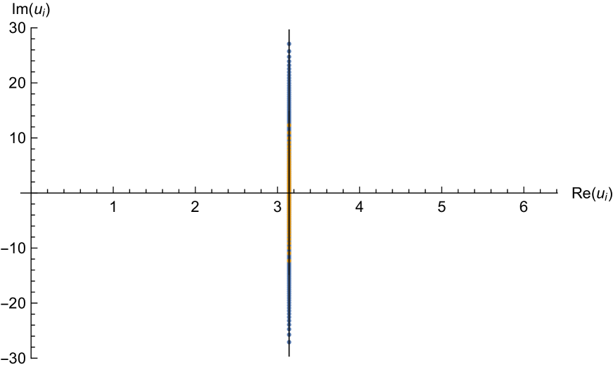
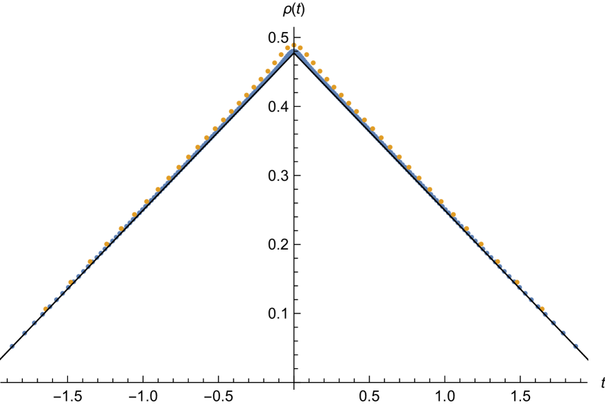
Refer to caption
(a) Eigenvalue distribution
Refer to caption
(b) Eigenvalue density ρ(t)𝜌𝑡\rho(t)
Refer to caption
Figure 16: Eigenvalues for the special case ΔX={2π3,2π3,2π3}subscriptΔ𝑋2𝜋32𝜋32𝜋3\Delta_{X}=\{\frac{2\pi}{3},\frac{2\pi}{3},\frac{2\pi}{3}\} for N=50𝑁50N=50 (orange) and 200200200 (blue) with the same other parameters.

Figure 16 shows that the real part of the eigenvalues is a constant. It is harder to spot the scaling from panel (a) but it is still N1/2superscript𝑁12N^{1/2}.

In Figure 18 we consider the effect of changing the number of flavors k𝑘k. As expected from the leading order solution [26], changing k𝑘k mostly affects the slope in the eigenvalue distribution ρ(t)𝜌𝑡\rho(t) which increases proportional to k𝑘k.

Refer to caption
(a) Eigenvalue distribution
Refer to caption
(b) Eigenvalue density ρ(t)𝜌𝑡\rho(t)
Refer to caption
Figure 18: Eigenvalues for the special case ΔX={2π3,2π3,2π3}subscriptΔ𝑋2𝜋32𝜋32𝜋3\Delta_{X}=\{\frac{2\pi}{3},\frac{2\pi}{3},\frac{2\pi}{3}\} for k=1𝑘1k=1 (blue), 222 (orange) and 333 (green) with the same other parameters.
Refer to caption
(a) Eigenvalue distribution
Refer to caption
(b) Eigenvalue density ρ(t)𝜌𝑡\rho(t)
Refer to caption
Figure 20: Eigenvalues for the special case ΔX={2π3,2π3,2π3}subscriptΔ𝑋2𝜋32𝜋32𝜋3\Delta_{X}=\{\frac{2\pi}{3},\frac{2\pi}{3},\frac{2\pi}{3}\} for {Δq,Δ~q}={2π3,4π3}subscriptΔ𝑞subscript~Δ𝑞2𝜋34𝜋3\{\Delta_{q},\tilde{\Delta}_{q}\}=\{-\frac{2\pi}{3},\frac{4\pi}{3}\} (blue), {π3,π3}𝜋3𝜋3\{\frac{\pi}{3},\frac{\pi}{3}\} (orange) and {2π3,0}2𝜋30\{\frac{2\pi}{3},0\} (green) with the same other parameters.

Figure 20 demonstrates that the role of the chemical potentials {Δq,Δ~q}subscriptΔ𝑞subscript~Δ𝑞\{\Delta_{q},\tilde{\Delta}_{q}\} display the real part of the eigenvalues uisubscript𝑢𝑖u_{i} and have, otherwise no effect on the imaginary eigenvalue density ρ(t)𝜌𝑡\rho(t).

Refer to caption
(a) Eigenvalue distribution
Refer to caption
(b) Eigenvalue density ρ(t)𝜌𝑡\rho(t)
Refer to caption
Figure 22: Eigenvalues for the special case Δm=0,ΔX={2π3,2π3,2π3}formulae-sequencesubscriptΔ𝑚0subscriptΔ𝑋2𝜋32𝜋32𝜋3\Delta_{m}=0,\Delta_{X}=\{\frac{2\pi}{3},\frac{2\pi}{3},\frac{2\pi}{3}\} (blue), and for the general cases Δm=π3,ΔX={π2,5π6,2π3}formulae-sequencesubscriptΔ𝑚𝜋3subscriptΔ𝑋𝜋25𝜋62𝜋3\Delta_{m}=-\frac{\pi}{3},\Delta_{X}=\{\frac{\pi}{2},\frac{5\pi}{6},\frac{2\pi}{3}\} (orange) and Δm=13,ΔX={53+2π3,53+2π3,2π3}formulae-sequencesubscriptΔ𝑚13subscriptΔ𝑋532𝜋3532𝜋32𝜋3\Delta_{m}=\frac{1}{3},\Delta_{X}=\{-\frac{5}{3}+\frac{2\pi}{3},\frac{5}{3}+\frac{2\pi}{3},\frac{2\pi}{3}\} (green) with the same other parameters.

Finally, we display the dependence of the eigenvalues uisubscript𝑢𝑖u_{i} on the choice of the chemical potential ΔXsubscriptΔ𝑋\Delta_{X} in Figure 22 keeping the same real parts.

4.2.2 The subleading term of the index at large N𝑁N

The index should take the form

RelogZ=f1(k,Δ,𝔫,𝔱)N3/2+f2(k,Δ,𝔫,𝔱)N1/2+f3(k,Δ,𝔫,𝔱)logN+f4(k,Δ,𝔫,𝔱)+𝒪(N1/2),Re𝑍subscript𝑓1𝑘Δ𝔫𝔱superscript𝑁32subscript𝑓2𝑘Δ𝔫𝔱superscript𝑁12subscript𝑓3𝑘Δ𝔫𝔱𝑁subscript𝑓4𝑘Δ𝔫𝔱𝒪superscript𝑁12{\rm Re}\log Z=f_{1}(k,\Delta,\mathfrak{n},\mathfrak{t})N^{3/2}+f_{2}(k,\Delta,\mathfrak{n},\mathfrak{t})N^{1/2}+f_{3}(k,\Delta,\mathfrak{n},\mathfrak{t})\log{N}+f_{4}(k,\Delta,\mathfrak{n},\mathfrak{t})+\mathcal{O}(N^{-1/2}), (4.28)

where the functions f1subscript𝑓1f_{1}, f2subscript𝑓2f_{2}, f3subscript𝑓3f_{3} and f4subscript𝑓4f_{4} are linear in the magnetic fluxes 𝔫𝔫\mathfrak{n} and 𝔱𝔱\mathfrak{t}.

The index Eq. (4.22) and RelogZRe𝑍{\rm Re}\log Z can be computed using the numerical solutions. For simplicity we set 𝔫qj=𝔫qsubscript𝔫subscript𝑞𝑗subscript𝔫𝑞\mathfrak{n}_{q_{j}}=\mathfrak{n}_{q} and 𝔫~qj=𝔫~qsubscript~𝔫subscript𝑞𝑗subscript~𝔫𝑞\tilde{\mathfrak{n}}_{q_{j}}=\tilde{\mathfrak{n}}_{q} for all j𝑗j. Under the similar decomposition

RelogZ=A+B1𝔫X1+B2𝔫q+B3𝔱,Re𝑍𝐴subscript𝐵1subscript𝔫subscript𝑋1subscript𝐵2subscript𝔫𝑞subscript𝐵3𝔱{\rm Re}\log Z=A+B_{1}\mathfrak{n}_{X_{1}}+B_{2}\mathfrak{n}_{q}+B_{3}\mathfrak{t}, (4.29)

where we have used the marginality condition on the superpotential 𝔫X1+𝔫X2=4/3subscript𝔫subscript𝑋1subscript𝔫subscript𝑋243\mathfrak{n}_{X_{1}}+\mathfrak{n}_{X_{2}}=4/3, 𝔫X3=2/3subscript𝔫subscript𝑋323\mathfrak{n}_{X_{3}}=2/3 and 𝔫q+𝔫~q=2/3subscript𝔫𝑞subscript~𝔫𝑞23\mathfrak{n}_{q}+\tilde{\mathfrak{n}}_{q}=2/3. Then we perform a linear least-squares fit for A𝐴A and Basubscript𝐵𝑎B_{a} to the function

f(N)=f1N3/2+f2N1/2+f3logN+f4+p=1pcfp+4N(12p)/2.𝑓𝑁subscript𝑓1superscript𝑁32subscript𝑓2superscript𝑁12subscript𝑓3𝑁subscript𝑓4superscriptsubscript𝑝1subscript𝑝𝑐subscript𝑓𝑝4superscript𝑁12𝑝2f(N)=f_{1}N^{3/2}+f_{2}N^{1/2}+f_{3}\log{N}+f_{4}+\sum_{p=1}^{p_{c}}f_{p+4}\,\,N^{\left(1-2p\right)/2}. (4.30)

The results of the numerical fit for RelogZRe𝑍{\rm Re}\log Z with N𝑁N are presented in Table 5. The analytical leading term computed by the index theorem in [26] and the numerical leading term f1N3/2subscript𝑓1superscript𝑁32f_{1}N^{3/2} match to number of significant digits present in the table. And the numerical results are also independent of {Δq,Δ~q}subscriptΔ𝑞subscript~Δ𝑞\{\Delta_{q},\tilde{\Delta}_{q}\}. The numerical results indicate that the coefficient f3subscript𝑓3f_{3} of the logN𝑁\log N term is precisely 1/212-1/2.

Furthermore, from the numerical results it is shown that by taking

ΔX1=Δ3,Δm=k(2π3Δ4),𝔫X1=𝔫3,𝔱=k[23(1g)𝔫4],formulae-sequencesubscriptΔsubscript𝑋1subscriptΔ3formulae-sequencesubscriptΔ𝑚𝑘2𝜋3subscriptΔ4formulae-sequencesubscript𝔫subscript𝑋1subscript𝔫3𝔱𝑘delimited-[]231𝑔subscript𝔫4\Delta_{X_{1}}=\Delta_{3},\quad\Delta_{m}=k\left(\frac{2\pi}{3}-\Delta_{4}\right),\quad\mathfrak{n}_{X_{1}}=\mathfrak{n}_{3},\quad\mathfrak{t}=-k\left[\frac{2}{3}\left(1-g\right)-\mathfrak{n}_{4}\right], (4.31)

where g𝑔g is the genus and g=0𝑔0g=0 for this case, Model I matches exactly with Model II for every term, including to logarithmic terms which are equal as they are independent of the chemical potentials of the magnetic charges.

(a) Δm=0subscriptΔ𝑚0\Delta_{m}=0;{ΔX1,ΔX2,ΔX3}={2π3,2π3,2π3}subscriptΔsubscript𝑋1subscriptΔsubscript𝑋2subscriptΔsubscript𝑋32𝜋32𝜋32𝜋3\,\{\Delta_{X_{1}},\Delta_{X_{2}},\Delta_{X_{3}}\}=\{\frac{2\pi}{3},\frac{2\pi}{3},\frac{2\pi}{3}\}.
k𝑘k ΔqsubscriptΔ𝑞\Delta_{q} Δ~qsubscript~Δ𝑞\tilde{\Delta}_{q} N(s)𝑁𝑠N(s) f1subscript𝑓1f_{1} f2subscript𝑓2f_{2} f3subscript𝑓3f_{3} f4subscript𝑓4f_{4}
111 2π32𝜋3-\frac{2\pi}{3} 4π34𝜋3\frac{4\pi}{3} 100300(10)similar-to10030010100\sim 300(10) 1.861681.86168-1.86168 +3.025263.02526+3.02526 0.500660.50066-0.50066 2.757402.75740-2.75740
π3𝜋3\frac{\pi}{3} π3𝜋3\frac{\pi}{3} 100300(10)similar-to10030010100\sim 300(10) 1.861681.86168-1.86168 +3.025263.02526+3.02526 0.500660.50066-0.50066 2.757402.75740-2.75740
2π32𝜋3\frac{2\pi}{3} 00 100300(10)similar-to10030010100\sim 300(10) 1.861681.86168-1.86168 +3.025263.02526+3.02526 0.500660.50066-0.50066 2.757402.75740-2.75740
222 2π32𝜋3-\frac{2\pi}{3} 4π34𝜋3\frac{4\pi}{3} 100200(5)similar-to1002005100\sim 200(5) 2.632822.63282-2.63282 +3.373343.37334+3.37334 0.500900.50090-0.50090 3.260963.26096-3.26096
333 2π32𝜋3-\frac{2\pi}{3} 4π34𝜋3\frac{4\pi}{3} 100200(5)similar-to1002005100\sim 200(5) 3.224533.22453-3.22453 +4.433784.43378+4.43378 0.501150.50115-0.50115 4.754534.75453-4.75453
(b) Δm=π3subscriptΔ𝑚𝜋3\Delta_{m}=-\frac{\pi}{3};{ΔX1,ΔX2,ΔX3}={π2,5π6,2π3}subscriptΔsubscript𝑋1subscriptΔsubscript𝑋2subscriptΔsubscript𝑋3𝜋25𝜋62𝜋3\,\{\Delta_{X_{1}},\Delta_{X_{2}},\Delta_{X_{3}}\}=\{\frac{\pi}{2},\frac{5\pi}{6},\frac{2\pi}{3}\}.
k𝑘k ΔqsubscriptΔ𝑞\Delta_{q} Δ~qsubscript~Δ𝑞\tilde{\Delta}_{q} N(s)𝑁𝑠N(s) f1subscript𝑓1f_{1} f2subscript𝑓2f_{2} f3subscript𝑓3f_{3} f4subscript𝑓4f_{4}
111 2π32𝜋3-\frac{2\pi}{3} 4π34𝜋3\frac{4\pi}{3} 100300(10)similar-to10030010100\sim 300(10)
1.665141.66514-1.66514
0.31221𝔫X10.31221subscript𝔫subscript𝑋1-0.31221\mathfrak{n}_{X_{1}}
+0.78053𝔱0.78053𝔱+0.78053\mathfrak{t}
+3.449993.44999+3.44999
+0.00781𝔫X10.00781subscript𝔫subscript𝑋1+0.00781\mathfrak{n}_{X_{1}}
0.17562𝔱0.17562𝔱-0.17562\mathfrak{t}
0.500820.50082-0.50082
3.267463.26746-3.26746
0.02821𝔫X10.02821subscript𝔫subscript𝑋1-0.02821\mathfrak{n}_{X_{1}}
+0.19180𝔱0.19180𝔱+0.19180\mathfrak{t}
π3𝜋3\frac{\pi}{3} π3𝜋3\frac{\pi}{3} 100300(10)similar-to10030010100\sim 300(10)
1.665141.66514-1.66514
0.31221𝔫X10.31221subscript𝔫subscript𝑋1-0.31221\mathfrak{n}_{X_{1}}
+0.78053𝔱0.78053𝔱+0.78053\mathfrak{t}
+3.449993.44999+3.44999
+0.00781𝔫X10.00781subscript𝔫subscript𝑋1+0.00781\mathfrak{n}_{X_{1}}
0.17562𝔱0.17562𝔱-0.17562\mathfrak{t}
0.500820.50082-0.50082
3.267463.26746-3.26746
0.02821𝔫X10.02821subscript𝔫subscript𝑋1-0.02821\mathfrak{n}_{X_{1}}
+0.19180𝔱0.19180𝔱+0.19180\mathfrak{t}
2π32𝜋3\frac{2\pi}{3} 00 100300(10)similar-to10030010100\sim 300(10)
1.665141.66514-1.66514
0.31221𝔫X10.31221subscript𝔫subscript𝑋1-0.31221\mathfrak{n}_{X_{1}}
+0.78053𝔱0.78053𝔱+0.78053\mathfrak{t}
+3.449993.44999+3.44999
+0.00781𝔫X10.00781subscript𝔫subscript𝑋1+0.00781\mathfrak{n}_{X_{1}}
0.17562𝔱0.17562𝔱-0.17562\mathfrak{t}
0.500820.50082-0.50082
3.267463.26746-3.26746
0.02821𝔫X10.02821subscript𝔫subscript𝑋1-0.02821\mathfrak{n}_{X_{1}}
+0.19180𝔱0.19180𝔱+0.19180\mathfrak{t}
222 2π32𝜋3-\frac{2\pi}{3} 4π34𝜋3\frac{4\pi}{3} 100200(5)similar-to1002005100\sim 200(5)
2.303722.30372-2.30372
0.49365𝔫X10.49365subscript𝔫subscript𝑋1-0.49365\mathfrak{n}_{X_{1}}
+0.24683𝔱0.24683𝔱+0.24683\mathfrak{t}
+3.192333.19233+3.19233
+0.41961𝔫X10.41961subscript𝔫subscript𝑋1+0.41961\mathfrak{n}_{X_{1}}
+0.08639𝔱0.08639𝔱+0.08639\mathfrak{t}
0.500980.50098-0.50098
3.220953.22095-3.22095
0.34133𝔫X10.34133subscript𝔫subscript𝑋1-0.34133\mathfrak{n}_{X_{1}}
0.06902𝔱0.06902𝔱-0.06902\mathfrak{t}
333 2π32𝜋3-\frac{2\pi}{3} 4π34𝜋3\frac{4\pi}{3} 100200(5)similar-to1002005100\sim 200(5)
2.814602.81460-2.81460
0.61569𝔫X10.61569subscript𝔫subscript𝑋1-0.61569\mathfrak{n}_{X_{1}}
+0.13193𝔱0.13193𝔱+0.13193\mathfrak{t}
+3.990133.99013+3.99013
+0.89056𝔫X10.89056subscript𝔫subscript𝑋1+0.89056\mathfrak{n}_{X_{1}}
+0.09188𝔱0.09188𝔱+0.09188\mathfrak{t}
0.501230.50123-0.50123
0.00006𝔫X10.00006subscript𝔫subscript𝑋1-0.00006\mathfrak{n}_{X_{1}}
+0.00003𝔱0.00003𝔱+0.00003\mathfrak{t}
4.526404.52640-4.52640
0.83862𝔫X10.83862subscript𝔫subscript𝑋1-0.83862\mathfrak{n}_{X_{1}}
0.08196𝔱0.08196𝔱-0.08196\mathfrak{t}
(c) Δm=13subscriptΔ𝑚13\Delta_{m}=\frac{1}{3};{ΔX1,ΔX2,ΔX3}={2π353,2π3+53,2π3}subscriptΔsubscript𝑋1subscriptΔsubscript𝑋2subscriptΔsubscript𝑋32𝜋3532𝜋3532𝜋3\,\{\Delta_{X_{1}},\Delta_{X_{2}},\Delta_{X_{3}}\}=\{\frac{2\pi}{3}-\frac{5}{3},\frac{2\pi}{3}+\frac{5}{3},\frac{2\pi}{3}\}.
k𝑘k ΔqsubscriptΔ𝑞\Delta_{q} Δ~qsubscript~Δ𝑞\tilde{\Delta}_{q} N(s)𝑁𝑠N(s) f1subscript𝑓1f_{1} f2subscript𝑓2f_{2} f3subscript𝑓3f_{3} f4subscript𝑓4f_{4}
111 2π32𝜋3-\frac{2\pi}{3} 4π34𝜋3\frac{4\pi}{3} 100200(5)similar-to1002005100\sim 200(5)
0.880900.88090-0.88090
1.81136𝔫X11.81136subscript𝔫subscript𝑋1-1.81136\mathfrak{n}_{X_{1}}
0.13631𝔱0.13631𝔱-0.13631\mathfrak{t}
+4.229924.22992+4.22992
+1.38166𝔫X11.38166subscript𝔫subscript𝑋1+1.38166\mathfrak{n}_{X_{1}}
0.06990𝔱0.06990𝔱-0.06990\mathfrak{t}
0.501680.50168-0.50168
0.00005𝔫X10.00005subscript𝔫subscript𝑋1-0.00005\mathfrak{n}_{X_{1}}
0.00001𝔱0.00001𝔱-0.00001\mathfrak{t}
4.497204.49720-4.49720
1.91182𝔫X11.91182subscript𝔫subscript𝑋1-1.91182\mathfrak{n}_{X_{1}}
+0.01935𝔱0.01935𝔱+0.01935\mathfrak{t}
222 2π32𝜋3-\frac{2\pi}{3} 4π34𝜋3\frac{4\pi}{3} 100200(5)similar-to1002005100\sim 200(5)
1.242271.24227-1.24227
2.58650𝔫X12.58650subscript𝔫subscript𝑋1-2.58650\mathfrak{n}_{X_{1}}
0.04773𝔱0.04773𝔱-0.04773\mathfrak{t}
+3.875993.87599+3.87599
+5.44770𝔫X15.44770subscript𝔫subscript𝑋1+5.44770\mathfrak{n}_{X_{1}}
0.07670𝔱0.07670𝔱-0.07670\mathfrak{t}
0.504090.50409-0.50409
+0.00620𝔫X10.00620subscript𝔫subscript𝑋1+0.00620\mathfrak{n}_{X_{1}}
+0.00063𝔱0.00063𝔱+0.00063\mathfrak{t}
5.286165.28616-5.28616
8.41742𝔫X18.41742subscript𝔫subscript𝑋1-8.41742\mathfrak{n}_{X_{1}}
+0.05162𝔱0.05162𝔱+0.05162\mathfrak{t}
333 2π32𝜋3-\frac{2\pi}{3} 4π34𝜋3\frac{4\pi}{3} 100200(5)similar-to1002005100\sim 200(5)
1.520701.52070-1.52070
3.17340𝔫X13.17340subscript𝔫subscript𝑋1-3.17340\mathfrak{n}_{X_{1}}
0.02594𝔱0.02594𝔱-0.02594\mathfrak{t}
+4.403374.40337+4.40337
+10.53032𝔫X110.53032subscript𝔫subscript𝑋1+10.53032\mathfrak{n}_{X_{1}}
0.06618𝔱0.06618𝔱-0.06618\mathfrak{t}
0.498270.49827-0.49827
0.05617𝔫X10.05617subscript𝔫subscript𝑋1-0.05617\mathfrak{n}_{X_{1}}
0.00672𝔱0.00672𝔱-0.00672\mathfrak{t}
7.734477.73447-7.73447
18.79411𝔫X118.79411subscript𝔫subscript𝑋1-18.79411\mathfrak{n}_{X_{1}}
+0.09834𝔱0.09834𝔱+0.09834\mathfrak{t}
Table 5: (V5,2superscript𝑉52V^{5,2} Model II) Numerical fit for RelogZ=f1N3/2+f2N1/2+f3logN+f4+g=1gc=5N(12g)/2Re𝑍subscript𝑓1superscript𝑁32subscript𝑓2superscript𝑁12subscript𝑓3𝑁subscript𝑓4superscriptsubscript𝑔1subscript𝑔𝑐5superscript𝑁12𝑔2{\rm Re}\log Z=f_{1}N^{3/2}+f_{2}N^{1/2}+f_{3}\log{N}+f_{4}+\sum_{g=1}^{g_{c}=5}N^{\left(1-2g\right)/2}.

5 The topologically twisted index of Q1,1,1superscript𝑄111Q^{1,1,1}

The field theory dual to M-theory of AdS×4Q1,1,1/k{}_{4}\times Q^{1,1,1}/\mathbb{Z}_{k} was originally discussed in [47, 43], see also [48]. The quiver diagram is a particular flavored type of the ABJM quiver:

(5.1)

with the superpotential

W𝑊\displaystyle W =\displaystyle= Tr(A1B1A2B2A1B2A2B1)Trsubscript𝐴1subscript𝐵1subscript𝐴2subscript𝐵2subscript𝐴1subscript𝐵2subscript𝐴2subscript𝐵1\displaystyle{\rm Tr}\left(A_{1}B_{1}A_{2}B_{2}-A_{1}B_{2}A_{2}B_{1}\right) (5.2)
+Tr[j=1na1qj(1)A1q~j(1)+j=1na2qj(2)A2q~j(2)+j=1nb1Qj(1)B1Q~j(1)+j=1nb2Qj(2)B2Q~j(2)].Trdelimited-[]superscriptsubscript𝑗1subscript𝑛𝑎1superscriptsubscript𝑞𝑗1subscript𝐴1superscriptsubscript~𝑞𝑗1superscriptsubscript𝑗1subscript𝑛𝑎2superscriptsubscript𝑞𝑗2subscript𝐴2superscriptsubscript~𝑞𝑗2superscriptsubscript𝑗1subscript𝑛𝑏1superscriptsubscript𝑄𝑗1subscript𝐵1superscriptsubscript~𝑄𝑗1superscriptsubscript𝑗1subscript𝑛𝑏2superscriptsubscript𝑄𝑗2subscript𝐵2superscriptsubscript~𝑄𝑗2\displaystyle+{\rm Tr}\left[\sum_{j=1}^{n_{a1}}q_{j}^{(1)}A_{1}\tilde{q}_{j}^{(1)}+\sum_{j=1}^{n_{a2}}q_{j}^{(2)}A_{2}\tilde{q}_{j}^{(2)}+\sum_{j=1}^{n_{b1}}Q_{j}^{(1)}B_{1}\tilde{Q}_{j}^{(1)}+\sum_{j=1}^{n_{b2}}Q_{j}^{(2)}B_{2}\tilde{Q}_{j}^{(2)}\right].

The free energy of the field theory on S3superscript𝑆3S^{3} was shown to match the gravity side in [44, 46]. Aspects of the superconformal index have been discussed in [39, 40]. The large N𝑁N analysis of the topologically twisted index was presented in [26] whose notation and leading order analysis we follow very closely.

5.1 Numerical solutions to the system of BAEs

From the ingredients of the quiver diagram 5.1 one constructs the topologically twisted index as

Z𝑍\displaystyle Z =\displaystyle= 1(N!)2𝔪,𝔪~N𝒞i=1Ndxi2πixidx~i2πix~ixi𝔱x~i𝔱~ξ𝔪iξ~𝔪~i×ijN(1xixj)(1x~ix~j)1superscript𝑁2subscript𝔪~𝔪superscript𝑁subscript𝒞superscriptsubscriptproduct𝑖1𝑁𝑑subscript𝑥𝑖2𝜋𝑖subscript𝑥𝑖𝑑subscript~𝑥𝑖2𝜋𝑖subscript~𝑥𝑖superscriptsubscript𝑥𝑖𝔱superscriptsubscript~𝑥𝑖~𝔱superscript𝜉subscript𝔪𝑖superscript~𝜉subscript~𝔪𝑖superscriptsubscriptproduct𝑖𝑗𝑁1subscript𝑥𝑖subscript𝑥𝑗1subscript~𝑥𝑖subscript~𝑥𝑗\displaystyle\frac{1}{(N!)^{2}}\sum\limits_{\mathfrak{m},\tilde{\mathfrak{m}}\in\mathbb{Z}^{N}}\int_{\cal C}\prod\limits_{i=1}^{N}\frac{dx_{i}}{2\pi ix_{i}}\frac{d\tilde{x}_{i}}{2\pi i\tilde{x}_{i}}x_{i}^{\mathfrak{t}}\tilde{x}_{i}^{\tilde{\mathfrak{t}}}\xi^{\mathfrak{m}_{i}}\tilde{\xi}^{-\tilde{\mathfrak{m}}_{i}}\times\prod\limits_{i\neq j}^{N}\left(1-\frac{x_{i}}{x_{j}}\right)\left(1-\frac{\tilde{x}_{i}}{\tilde{x}_{j}}\right) (5.3)
×i,j=1Na=1,2(xix~jya1xix~jya)𝔪i𝔪~j𝔫a+1b=3,4(x~jxiyb1x~jxiyb)𝔪~j𝔪i𝔫b+1\displaystyle\times\prod\limits_{i,j=1}^{N}\prod\limits_{a=1,2}\left(\frac{\sqrt{\frac{x_{i}}{\tilde{x}_{j}}y_{a}}}{1-\frac{x_{i}}{\tilde{x}_{j}}y_{a}}\right)^{\mathfrak{m}_{i}-\tilde{\mathfrak{m}}_{j}-\mathfrak{n}_{a}+1}\prod\limits_{b=3,4}\left(\frac{\sqrt{\frac{\tilde{x}_{j}}{x_{i}}y_{b}}}{1-\frac{\tilde{x}_{j}}{x_{i}}y_{b}}\right)^{\tilde{\mathfrak{m}}_{j}-\mathfrak{m}_{i}-\mathfrak{n}_{b}+1}
×i=1Nk=1,2(1xiy~ak11xiy~ak)n(𝔪i𝔫~ak+1)×j=1Nk=1,2(x~jyak1x~jyak)n(𝔪~j𝔫ak+1).\displaystyle\times\prod\limits_{i=1}^{N}\prod\limits_{k=1,2}\Bigg{(}\frac{\sqrt{\frac{1}{x_{i}}\tilde{y}_{ak}}}{1-\frac{1}{x_{i}}\tilde{y}_{ak}}\Bigg{)}^{n(-\mathfrak{m}_{i}-\tilde{\mathfrak{n}}_{ak}+1)}\times\prod\limits_{j=1}^{N}\prod\limits_{k=1,2}\Bigg{(}\frac{\sqrt{\tilde{x}_{j}y_{ak}}}{1-\tilde{x}_{j}y_{ak}}\Bigg{)}^{n(\tilde{\mathfrak{m}}_{j}-\mathfrak{n}_{ak}+1)}.

Permorming the summation over magnetic fluxes introducing a large cut-off M𝑀M.

Z𝑍\displaystyle Z =\displaystyle= 1(N!)2𝔪,𝔪~N𝒞i=1Ndxi2πixidx~i2πix~ixi𝔱x~i𝔱~×ijN(1xixj)(1x~ix~j)1superscript𝑁2subscript𝔪~𝔪superscript𝑁subscript𝒞superscriptsubscriptproduct𝑖1𝑁𝑑subscript𝑥𝑖2𝜋𝑖subscript𝑥𝑖𝑑subscript~𝑥𝑖2𝜋𝑖subscript~𝑥𝑖superscriptsubscript𝑥𝑖𝔱superscriptsubscript~𝑥𝑖~𝔱superscriptsubscriptproduct𝑖𝑗𝑁1subscript𝑥𝑖subscript𝑥𝑗1subscript~𝑥𝑖subscript~𝑥𝑗\displaystyle\frac{1}{(N!)^{2}}\sum\limits_{\mathfrak{m},\tilde{\mathfrak{m}}\in\mathbb{Z}^{N}}\int_{\cal C}\prod\limits_{i=1}^{N}\frac{dx_{i}}{2\pi ix_{i}}\frac{d\tilde{x}_{i}}{2\pi i\tilde{x}_{i}}x_{i}^{\mathfrak{t}}\tilde{x}_{i}^{\tilde{\mathfrak{t}}}\times\prod\limits_{i\neq j}^{N}\left(1-\frac{x_{i}}{x_{j}}\right)\left(1-\frac{\tilde{x}_{i}}{\tilde{x}_{j}}\right) (5.4)
×i,j=1Na=1,2(xix~jya1xix~jya)1𝔫ab=3,4(x~jxiyb1x~jxiyb)1𝔫b\displaystyle\times\prod\limits_{i,j=1}^{N}\prod\limits_{a=1,2}\left(\frac{\sqrt{\frac{x_{i}}{\tilde{x}_{j}}y_{a}}}{1-\frac{x_{i}}{\tilde{x}_{j}}y_{a}}\right)^{1-\mathfrak{n}_{a}}\prod\limits_{b=3,4}\left(\frac{\sqrt{\frac{\tilde{x}_{j}}{x_{i}}y_{b}}}{1-\frac{\tilde{x}_{j}}{x_{i}}y_{b}}\right)^{1-\mathfrak{n}_{b}}
×i=1Nk=1,2(1xiy~ak11xiy~ak)n(1𝔫~ak)×j=1Nk=1,2(x~jyak1x~jyak)n(1𝔫ak)\displaystyle\times\prod\limits_{i=1}^{N}\prod\limits_{k=1,2}\Bigg{(}\frac{\sqrt{\frac{1}{x_{i}}\tilde{y}_{ak}}}{1-\frac{1}{x_{i}}\tilde{y}_{ak}}\Bigg{)}^{n(1-\tilde{\mathfrak{n}}_{ak})}\times\prod\limits_{j=1}^{N}\prod\limits_{k=1,2}\Bigg{(}\frac{\sqrt{\tilde{x}_{j}y_{ak}}}{1-\tilde{x}_{j}y_{ak}}\Bigg{)}^{n(1-\mathfrak{n}_{ak})}
×i=1N(eiBi)MeiBi1j=1N(eiB~j)MeiB~j1,\displaystyle\times\prod\limits_{i=1}^{N}\frac{\big{(}e^{iB_{i}}\big{)}^{M}}{e^{iB_{i}}-1}\prod\limits_{j=1}^{N}\frac{\big{(}e^{i\tilde{B}_{j}}\big{)}^{M}}{e^{i\tilde{B}_{j}}-1},

where the Bethe Ansatz equations are

11\displaystyle 1 =\displaystyle= eiBi=ξj=1N(1y3x~jxi)(1y4x~jxi)(1y11x~jxi)(1y21x~jxi)×k=1,2(1xiy~ak11xiy~ak)n,superscript𝑒𝑖subscript𝐵𝑖𝜉superscriptsubscriptproduct𝑗1𝑁1subscript𝑦3subscript~𝑥𝑗subscript𝑥𝑖1subscript𝑦4subscript~𝑥𝑗subscript𝑥𝑖1superscriptsubscript𝑦11subscript~𝑥𝑗subscript𝑥𝑖1superscriptsubscript𝑦21subscript~𝑥𝑗subscript𝑥𝑖subscriptproduct𝑘12superscript1subscript𝑥𝑖subscript~𝑦𝑎𝑘11subscript𝑥𝑖subscript~𝑦𝑎𝑘𝑛\displaystyle e^{iB_{i}}=\xi\prod\limits_{j=1}^{N}\frac{\left(1-y_{3}\frac{\tilde{x}_{j}}{x_{i}}\right)\left(1-y_{4}\frac{\tilde{x}_{j}}{x_{i}}\right)}{\left(1-y_{1}^{-1}\frac{\tilde{x}_{j}}{x_{i}}\right)\left(1-y_{2}^{-1}\frac{\tilde{x}_{j}}{x_{i}}\right)}\times\prod\limits_{k=1,2}\Bigg{(}\frac{\sqrt{\frac{1}{x_{i}}\tilde{y}_{ak}}}{1-\frac{1}{x_{i}}\tilde{y}_{ak}}\Bigg{)}^{-n},
11\displaystyle 1 =\displaystyle= eiB~j=ξ~i=1N(1y3x~jxi)(1y4x~jxi)(1y11x~jxi)(1y21x~jxi)×k=1,2(x~jyak1x~jyak)n.superscript𝑒𝑖subscript~𝐵𝑗~𝜉superscriptsubscriptproduct𝑖1𝑁1subscript𝑦3subscript~𝑥𝑗subscript𝑥𝑖1subscript𝑦4subscript~𝑥𝑗subscript𝑥𝑖1superscriptsubscript𝑦11subscript~𝑥𝑗subscript𝑥𝑖1superscriptsubscript𝑦21subscript~𝑥𝑗subscript𝑥𝑖subscriptproduct𝑘12superscriptsubscript~𝑥𝑗subscript𝑦𝑎𝑘1subscript~𝑥𝑗subscript𝑦𝑎𝑘𝑛\displaystyle e^{i\tilde{B}_{j}}=\tilde{\xi}\prod\limits_{i=1}^{N}\frac{\left(1-y_{3}\frac{\tilde{x}_{j}}{x_{i}}\right)\left(1-y_{4}\frac{\tilde{x}_{j}}{x_{i}}\right)}{\left(1-y_{1}^{-1}\frac{\tilde{x}_{j}}{x_{i}}\right)\left(1-y_{2}^{-1}\frac{\tilde{x}_{j}}{x_{i}}\right)}\times\prod\limits_{k=1,2}\Bigg{(}\frac{\sqrt{\tilde{x}_{j}y_{ak}}}{1-\tilde{x}_{j}y_{ak}}\Bigg{)}^{-n}. (5.5)

The compact expression is

Z(ya,𝔫a)𝑍subscript𝑦𝑎subscript𝔫𝑎\displaystyle Z\left(y_{a},\mathfrak{n}_{a}\right) =\displaystyle= k=1,2[y~ak12Nn(1𝔫~ak)yak12Nn(1𝔫ak)]×a=14ya12N2𝔫asubscriptproduct𝑘12delimited-[]superscriptsubscript~𝑦𝑎𝑘12𝑁𝑛1subscript~𝔫𝑎𝑘superscriptsubscript𝑦𝑎𝑘12𝑁𝑛1subscript𝔫𝑎𝑘superscriptsubscriptproduct𝑎14superscriptsubscript𝑦𝑎12superscript𝑁2subscript𝔫𝑎\displaystyle\prod\limits_{k=1,2}\left[{\tilde{y}_{ak}}^{\frac{1}{2}Nn\left(1-\tilde{\mathfrak{n}}_{ak}\right)}y_{ak}^{\frac{1}{2}Nn\left(1-\mathfrak{n}_{ak}\right)}\right]\times\prod_{a=1}^{4}y_{a}^{-\frac{1}{2}N^{2}\mathfrak{n}_{a}} (5.6)
×IBAE[1det𝔹i=1NxiN+𝔱x~iN+𝔱~ij(1xixj)(1x~ix~j)i,j=1Na=1,2(x~jyaxi)1𝔫aa=3,4(xiyax~j)1𝔫a\displaystyle\times\sum_{I\in BAE}\left[\frac{1}{\det\mathbb{B}}\frac{\prod_{i=1}^{N}x_{i}^{N+\mathfrak{t}}\tilde{x}_{i}^{N+\tilde{\mathfrak{t}}}\prod_{i\neq j}\left(1-\frac{x_{i}}{x_{j}}\right)\left(1-\frac{\tilde{x}_{i}}{\tilde{x}_{j}}\right)}{\prod_{i,j=1}^{N}\prod_{a=1,2}\left(\tilde{x}_{j}-y_{a}x_{i}\right)^{1-\mathfrak{n}_{a}}\prod_{a=3,4}\left(x_{i}-y_{a}\tilde{x}_{j}\right)^{1-\mathfrak{n}_{a}}}\right.
×i=1Nk=1,2xi12n(1𝔫~ak)x~i12n(1𝔫ak)(xiy~ak)n(1𝔫~ak)(1x~iyak)n(1𝔫ak)].\displaystyle\left.\times\prod_{i=1}^{N}\prod\limits_{k=1,2}\frac{x_{i}^{\frac{1}{2}n(1-\tilde{\mathfrak{n}}_{ak})}\tilde{x}_{i}^{\frac{1}{2}n(1-\mathfrak{n}_{ak})}}{\left(x_{i}-\tilde{y}_{ak}\right)^{n(1-\tilde{\mathfrak{n}}_{ak})}\left(1-\tilde{x}_{i}y_{ak}\right)^{n(1-\mathfrak{n}_{ak})}}\right].

The matrix 𝔹𝔹\mathbb{B} is

𝔹|BAEs=(δjl[m=1NGjm+k=1,2nxjxjy~akn]GjlGljδjl[m=1NGmj+k=1,2nx~jx~jyak1n]).evaluated-at𝔹BAEssubscript𝛿𝑗𝑙delimited-[]superscriptsubscript𝑚1𝑁subscript𝐺𝑗𝑚subscript𝑘12𝑛subscript𝑥𝑗subscript𝑥𝑗subscript~𝑦𝑎𝑘𝑛subscript𝐺𝑗𝑙subscript𝐺𝑙𝑗subscript𝛿𝑗𝑙delimited-[]superscriptsubscript𝑚1𝑁subscript𝐺𝑚𝑗subscript𝑘12𝑛subscript~𝑥𝑗subscript~𝑥𝑗superscriptsubscript𝑦𝑎𝑘1𝑛\mathbb{B}\Big{|}_{\rm BAEs}=\left(\begin{array}[]{cc}\delta_{jl}\left[-\sum\limits_{m=1}^{N}G_{jm}+\sum\limits_{k=1,2}\frac{nx_{j}}{x_{j}-\tilde{y}_{ak}}-n\right]&G_{jl}\\ -G_{lj}&\delta_{jl}\left[\sum\limits_{m=1}^{N}G_{mj}+\sum\limits_{k=1,2}\frac{n\tilde{x}_{j}}{\tilde{x}_{j}-y_{ak}^{-1}}-n\right]\end{array}\right). (5.7)

The Bethe potential is

𝒱𝒱\displaystyle\mathcal{V} =\displaystyle= i=1N[Δm(1)ui+Δm(2)u~i2π(n~iu~iniui)]superscriptsubscript𝑖1𝑁delimited-[]superscriptsubscriptΔ𝑚1subscript𝑢𝑖superscriptsubscriptΔ𝑚2subscript~𝑢𝑖2𝜋subscript~𝑛𝑖subscript~𝑢𝑖subscript𝑛𝑖subscript𝑢𝑖\displaystyle\sum\limits_{i=1}^{N}\left[-\Delta_{m}^{(1)}u_{i}+\Delta_{m}^{(2)}\tilde{u}_{i}-2\pi\left(\tilde{n}_{i}\tilde{u}_{i}-n_{i}u_{i}\right)\right] (5.8)
+i,j=1N[a=3,4Li2(ei(u~jui+Δa))a=1,2Li2(ei(u~juiΔa))]superscriptsubscript𝑖𝑗1𝑁delimited-[]subscript𝑎34subscriptLi2superscript𝑒𝑖subscript~𝑢𝑗subscript𝑢𝑖subscriptΔ𝑎subscript𝑎12subscriptLi2superscript𝑒𝑖subscript~𝑢𝑗subscript𝑢𝑖subscriptΔ𝑎\displaystyle+\sum\limits_{i,j=1}^{N}\left[\sum\limits_{a=3,4}{\rm Li}_{2}\left(e^{i\left(\tilde{u}_{j}-u_{i}+\Delta_{a}\right)}\right)-\sum\limits_{a=1,2}{\rm Li}_{2}\left(e^{i\left(\tilde{u}_{j}-u_{i}-\Delta_{a}\right)}\right)\right]
+ni=1Nk=1,2[Li2(ei(ui+Δ~ak))Li2(ei(u~iΔak))]𝑛superscriptsubscript𝑖1𝑁subscript𝑘12delimited-[]subscriptLi2superscript𝑒𝑖subscript𝑢𝑖subscript~Δ𝑎𝑘subscriptLi2superscript𝑒𝑖subscript~𝑢𝑖subscriptΔ𝑎𝑘\displaystyle+n\sum\limits_{i=1}^{N}\sum\limits_{k=1,2}\left[{\rm Li}_{2}\left(e^{i\left(-u_{i}+\tilde{\Delta}_{ak}\right)}\right)-{\rm Li}_{2}\left(e^{i\left(-\tilde{u}_{i}-\Delta_{ak}\right)}\right)\right]
+n2i=1Nk=1,2[(Δ~akπ)ui+(Δakπ)u~i]n2i=1N[ui2u~i2],𝑛2superscriptsubscript𝑖1𝑁subscript𝑘12delimited-[]subscript~Δ𝑎𝑘𝜋subscript𝑢𝑖subscriptΔ𝑎𝑘𝜋subscript~𝑢𝑖𝑛2superscriptsubscript𝑖1𝑁delimited-[]superscriptsubscript𝑢𝑖2superscriptsubscript~𝑢𝑖2\displaystyle+\frac{n}{2}\sum\limits_{i=1}^{N}\sum\limits_{k=1,2}\left[\left(\tilde{\Delta}_{ak}-\pi\right)u_{i}+\left(\Delta_{ak}-\pi\right)\tilde{u}_{i}\right]-\frac{n}{2}\sum\limits_{i=1}^{N}\left[u_{i}^{2}-\tilde{u}_{i}^{2}\right],

where

i=1N[2π(n~iu~iniui)]=(4πa=14Δa)i>jN(u~jui)=2πi>jN(u~jui).superscriptsubscript𝑖1𝑁delimited-[]2𝜋subscript~𝑛𝑖subscript~𝑢𝑖subscript𝑛𝑖subscript𝑢𝑖4𝜋superscriptsubscript𝑎14subscriptΔ𝑎superscriptsubscript𝑖𝑗𝑁subscript~𝑢𝑗subscript𝑢𝑖2𝜋superscriptsubscript𝑖𝑗𝑁subscript~𝑢𝑗subscript𝑢𝑖\sum\limits_{i=1}^{N}\left[-2\pi\left(\tilde{n}_{i}\tilde{u}_{i}-n_{i}u_{i}\right)\right]=\left(4\pi-\sum\limits_{a=1}^{4}\Delta_{a}\right)\sum\limits_{i>j}^{N}\left(\tilde{u}_{j}-u_{i}\right)=2\pi\sum\limits_{i>j}^{N}\left(\tilde{u}_{j}-u_{i}\right). (5.9)

It is assumed that 0<v(t)+Δ~a1<2π0𝑣𝑡subscript~Δ𝑎12𝜋0<-v(t)+\tilde{\Delta}_{a1}<2\pi, 0<v(t)+Δ~a2<2π0𝑣𝑡subscript~Δ𝑎22𝜋0<-v(t)+\tilde{\Delta}_{a2}<2\pi, 0<v~(t)+Δa1<2π0~𝑣𝑡subscriptΔ𝑎12𝜋0<\tilde{v}(t)+\Delta_{a1}<2\pi and 0<v~(t)+Δa2<2π0~𝑣𝑡subscriptΔ𝑎22𝜋0<\tilde{v}(t)+\Delta_{a2}<2\pi. Using Δ1=Δ2=πΔ3=πΔ4=ΔsubscriptΔ1subscriptΔ2𝜋subscriptΔ3𝜋subscriptΔ4Δ\Delta_{1}=\Delta_{2}=\pi-\Delta_{3}=\pi-\Delta_{4}=\Delta and the marginality condition from the superpotential Δ1+Δa1+Δ~a1=2πsubscriptΔ1subscriptΔ𝑎1subscript~Δ𝑎12𝜋\Delta_{1}+\Delta_{a1}+\tilde{\Delta}_{a1}=2\pi, Δ2+Δa2+Δ~a2=2πsubscriptΔ2subscriptΔ𝑎2subscript~Δ𝑎22𝜋\Delta_{2}+\Delta_{a2}+\tilde{\Delta}_{a2}=2\pi we get

v(t)+v~(t)2{(Δ2Δa12,+Δ+2Δ~a22),Δa1<Δa2(Δ2Δa22,+Δ+2Δ~a12),Δa1Δa2\frac{v(t)+\tilde{v}(t)}{2}\in\left\{\begin{aligned} \left(\frac{-\Delta-2\Delta_{a1}}{2},\frac{+\Delta+2\tilde{\Delta}_{a2}}{2}\right),\quad\Delta_{a1}<\Delta_{a2}\\ \left(\frac{-\Delta-2\Delta_{a2}}{2},\frac{+\Delta+2\tilde{\Delta}_{a1}}{2}\right),\quad\Delta_{a1}\geq\Delta_{a2}\end{aligned}\right. (5.10)

Thus we set the initial real part axis to be

v(t)+v~(t)2=2πΔΔa1Δa22.𝑣𝑡~𝑣𝑡22𝜋ΔsubscriptΔ𝑎1subscriptΔ𝑎22\frac{v(t)+\tilde{v}(t)}{2}=\frac{2\pi-\Delta-\Delta_{a1}-\Delta_{a2}}{2}. (5.11)

Note that we have specialized from the general flavored ABJM quiver 5.1 to the particular case corresponding to the dual of AdS×4Q1,1,1/n{}_{4}\times Q^{1,1,1}/\mathbb{Z}_{n} which in the notation we have introduced implies: k=0,na1=na2=n,nb1=nb2=0formulae-sequenceformulae-sequence𝑘0subscript𝑛𝑎1subscript𝑛𝑎2𝑛subscript𝑛𝑏1subscript𝑛𝑏20k=0,n_{a1}=n_{a2}=n,n_{b1}=n_{b2}=0 where the subindex bi𝑏𝑖bi corresponds to the fields Q𝑄Q and Q~~𝑄\tilde{Q}. Our goal is thus, to explore the numerical behavior of the index as a function of N𝑁N and ΔasubscriptΔ𝑎\Delta_{a} just as in the ABJM case but also as functions of {Δm(1),Δm(2)}superscriptsubscriptΔ𝑚1superscriptsubscriptΔ𝑚2\{\Delta_{m}^{(1)},\Delta_{m}^{(2)}\}, n𝑛n and {Δa1,Δa2,Δ~a1,Δ~a2}subscriptΔ𝑎1subscriptΔ𝑎2subscript~Δ𝑎1subscript~Δ𝑎2\{\Delta_{a1},\Delta_{a2},\tilde{\Delta}_{a1},\tilde{\Delta}_{a2}\}.

We set Δm=Δm(2)Δm(1)subscriptΔ𝑚superscriptsubscriptΔ𝑚2superscriptsubscriptΔ𝑚1\Delta_{m}=\Delta_{m}^{(2)}-\Delta_{m}^{(1)}. The numerical solutions for different values of N𝑁N, n𝑛n, {Δm(1),Δm(2)}superscriptsubscriptΔ𝑚1superscriptsubscriptΔ𝑚2\{\Delta_{m}^{(1)},\Delta_{m}^{(2)}\}, ΔmsubscriptΔ𝑚\Delta_{m}, {Δa1,Δa2,Δ~a1,Δ~a2}subscriptΔ𝑎1subscriptΔ𝑎2subscript~Δ𝑎1subscript~Δ𝑎2\{\Delta_{a1},\Delta_{a2},\tilde{\Delta}_{a1},\tilde{\Delta}_{a2}\} and Δa={Δ1,Δ2,Δ3,Δ4}(Δ)subscriptΔ𝑎subscriptΔ1subscriptΔ2subscriptΔ3subscriptΔ4Δ\Delta_{a}=\{\Delta_{1},\Delta_{2},\Delta_{3},\Delta_{4}\}(\Delta) are shown in Figures 24 - 34.

Let us briefly summarize the salient features of the exact eigenvalues that we find. Similar to the index of N0,1,0superscript𝑁010N^{0,1,0} in section 3.1, the eigenvalues are not reflectively symmetric about a particular real axis, except for the case that (Δm(1)+Δm(2))/2=πsuperscriptsubscriptΔ𝑚1superscriptsubscriptΔ𝑚22𝜋(\Delta_{m}^{(1)}+\Delta_{m}^{(2)})/2=\pi. Furthermore, the imaginary part of uisubscript𝑢𝑖u_{i} is not exactly the same as u~isubscript~𝑢𝑖\tilde{u}_{i} so that there are two numerical results of the eigenvalue density ρ(t)𝜌𝑡\rho(t), the real part difference δv(t)𝛿𝑣𝑡\delta v(t) and the real part axis (v(t)+v~(t))/2𝑣𝑡~𝑣𝑡2\left(v(t)+\tilde{v}(t)\right)/2. In addition, Figure 28 and Figure 32 show that the values of {Δm(1),Δm(2)}superscriptsubscriptΔ𝑚1superscriptsubscriptΔ𝑚2\{\Delta_{m}^{(1)},\Delta_{m}^{(2)}\} keeping the same ΔmsubscriptΔ𝑚\Delta_{m} and the values of {Δa1,Δa2,Δ~a1,Δ~a2}subscriptΔ𝑎1subscriptΔ𝑎2subscript~Δ𝑎1subscript~Δ𝑎2\{\Delta_{a1},\Delta_{a2},\tilde{\Delta}_{a1},\tilde{\Delta}_{a2}\} have effects only on the real part axis (v(t)+v~(t))/2𝑣𝑡~𝑣𝑡2\left(v(t)+\tilde{v}(t)\right)/2.

5.2 The subleading term of the index at large N𝑁N

The index should take the form

RelogZ=f1(n,Δ,𝔫,𝔱)N3/2+f2(n,Δ,𝔫,𝔱)N1/2+f3(n,Δ,𝔫,𝔱)logN+f4(n,Δ,𝔫,𝔱)+𝒪(N1/2),Re𝑍subscript𝑓1𝑛Δ𝔫𝔱superscript𝑁32subscript𝑓2𝑛Δ𝔫𝔱superscript𝑁12subscript𝑓3𝑛Δ𝔫𝔱𝑁subscript𝑓4𝑛Δ𝔫𝔱𝒪superscript𝑁12{\rm Re}\log Z=f_{1}(n,\Delta,\mathfrak{n},\mathfrak{t})N^{3/2}+f_{2}(n,\Delta,\mathfrak{n},\mathfrak{t})N^{1/2}+f_{3}(n,\Delta,\mathfrak{n},\mathfrak{t})\log{N}+f_{4}(n,\Delta,\mathfrak{n},\mathfrak{t})+\mathcal{O}(N^{-1/2}), (5.12)

where here ΔΔ\Delta represents all of the chemical potentials as above and the functions f1subscript𝑓1f_{1}, f2subscript𝑓2f_{2}, f3subscript𝑓3f_{3} and f4subscript𝑓4f_{4} are linear in the magnetic fluxes 𝔫𝔫\mathfrak{n} and 𝔱𝔱\mathfrak{t}.

The index Eq. (5.6) and RelogZRe𝑍{\rm Re}\log Z can be computed using the numerical solutions. Under the similar decomposition

RelogZ=A+B1𝔫1+B2𝔫2+B3𝔫3+B4𝔫a1+B5𝔫a2+B6𝔱+B7𝔱~,Re𝑍𝐴subscript𝐵1subscript𝔫1subscript𝐵2subscript𝔫2subscript𝐵3subscript𝔫3subscript𝐵4subscript𝔫𝑎1subscript𝐵5subscript𝔫𝑎2subscript𝐵6𝔱subscript𝐵7~𝔱{\rm Re}\log Z=A+B_{1}\mathfrak{n}_{1}+B_{2}\mathfrak{n}_{2}+B_{3}\mathfrak{n}_{3}+B_{4}\mathfrak{n}_{a1}+B_{5}\mathfrak{n}_{a2}+B_{6}\mathfrak{t}+B_{7}\tilde{\mathfrak{t}}, (5.13)

where we have used the marginality condition on the superpotential a=14𝔫a=2superscriptsubscript𝑎14subscript𝔫𝑎2\sum_{a=1}^{4}\mathfrak{n}_{a}=2, 𝔫1+𝔫a1+𝔫~a1=2subscript𝔫1subscript𝔫𝑎1subscript~𝔫𝑎12\mathfrak{n}_{1}+\mathfrak{n}_{a1}+\tilde{\mathfrak{n}}_{a1}=2 and 𝔫2+𝔫a2+𝔫~a2=2subscript𝔫2subscript𝔫𝑎2subscript~𝔫𝑎22\mathfrak{n}_{2}+\mathfrak{n}_{a2}+\tilde{\mathfrak{n}}_{a2}=2. Then we perform a linear least-squares fit for A𝐴A and Basubscript𝐵𝑎B_{a} to the function

f(N)=f1N3/2+f2N1/2+f3logN+f4+p=1pcfp+4N(12p)/2.𝑓𝑁subscript𝑓1superscript𝑁32subscript𝑓2superscript𝑁12subscript𝑓3𝑁subscript𝑓4superscriptsubscript𝑝1subscript𝑝𝑐subscript𝑓𝑝4superscript𝑁12𝑝2f(N)=f_{1}N^{3/2}+f_{2}N^{1/2}+f_{3}\log{N}+f_{4}+\sum_{p=1}^{p_{c}}f_{p+4}\,\,N^{\left(1-2p\right)/2}. (5.14)

The results of the numerical fit for RelogZRe𝑍{\rm Re}\log Z with N𝑁N are presented in Table 7. The analytical leading term computed by the index theorem in [26] and the numerical leading term f1N3/2subscript𝑓1superscript𝑁32f_{1}N^{3/2} match to number of significant digits present in the table. And the leading term is indeed independent of {Δm(1),Δm(2)}superscriptsubscriptΔ𝑚1superscriptsubscriptΔ𝑚2\{\Delta_{m}^{(1)},\Delta_{m}^{(2)}\} keeping the same ΔmsubscriptΔ𝑚\Delta_{m}, and {Δa1,Δa2,Δ~a1,Δ~a2}subscriptΔ𝑎1subscriptΔ𝑎2subscript~Δ𝑎1subscript~Δ𝑎2\{\Delta_{a1},\Delta_{a2},\tilde{\Delta}_{a1},\tilde{\Delta}_{a2}\}. The numerical results indicate that the coefficient f3subscript𝑓3f_{3} of the logN𝑁\log N term is precisely 1/212-1/2.

Refer to caption
(a) Eigenvalue distribution
Refer to caption
(b) Eigenvalue density ρ(t)𝜌𝑡\rho(t)
Refer to caption
(c) Real part difference δv(t)𝛿𝑣𝑡\delta v(t)
Refer to caption
(d) Real part axis (v(t)+v~(t))/2𝑣𝑡~𝑣𝑡2(v(t)+\tilde{v}(t))/2
Refer to caption
Figure 24: Eigenvalues for Δa={π2,π2,π2,π2}subscriptΔ𝑎𝜋2𝜋2𝜋2𝜋2\Delta_{a}=\{\frac{\pi}{2},\frac{\pi}{2},\frac{\pi}{2},\frac{\pi}{2}\} for N=50𝑁50N=50 (blue) and 200200200 (orange) with the same other parameters.
Refer to caption
(a) Eigenvalue distribution
Refer to caption
(b) Eigenvalue density ρ(t)𝜌𝑡\rho(t)
Refer to caption
(c) Real part difference δv(t)𝛿𝑣𝑡\delta v(t)
Refer to caption
(d) Real part axis (v(t)+v~(t))/2𝑣𝑡~𝑣𝑡2(v(t)+\tilde{v}(t))/2
Refer to caption
Figure 26: Eigenvalues for Δa={π2,π2,π2,π2}subscriptΔ𝑎𝜋2𝜋2𝜋2𝜋2\Delta_{a}=\{\frac{\pi}{2},\frac{\pi}{2},\frac{\pi}{2},\frac{\pi}{2}\} for n=1𝑛1n=1 (blue), 222 (orange) and 333 (green) with the same other parameters.
Refer to caption
(a) Eigenvalue distribution
Refer to caption
(b) Eigenvalue density ρ(t)𝜌𝑡\rho(t)
Refer to caption
(c) Real part difference δv(t)𝛿𝑣𝑡\delta v(t)
Refer to caption
(d) Real part axis (v(t)+v~(t))/2𝑣𝑡~𝑣𝑡2(v(t)+\tilde{v}(t))/2
Refer to caption
Figure 28: Eigenvalues for Δa={π2,π2,π2,π2}subscriptΔ𝑎𝜋2𝜋2𝜋2𝜋2\Delta_{a}=\{\frac{\pi}{2},\frac{\pi}{2},\frac{\pi}{2},\frac{\pi}{2}\} for {Δm(1),Δm(2)}={0,0}superscriptsubscriptΔ𝑚1superscriptsubscriptΔ𝑚200\{\Delta_{m}^{(1)},\Delta_{m}^{(2)}\}=\{0,0\} (blue), {π2,π2}𝜋2𝜋2\{\frac{\pi}{2},\frac{\pi}{2}\} (orange) and {π,π}𝜋𝜋\{\pi,\pi\} (green) keeping the same Δm=0subscriptΔ𝑚0\Delta_{m}=0 with the same other parameters.
Refer to caption
(a) Eigenvalue distribution
Refer to caption
(b) Eigenvalue density ρ(t)𝜌𝑡\rho(t)
Refer to caption
(c) Real part difference δv(t)𝛿𝑣𝑡\delta v(t)
Refer to caption
(d) Real part axis (v(t)+v~(t))/2𝑣𝑡~𝑣𝑡2(v(t)+\tilde{v}(t))/2
Refer to caption
Figure 30: Eigenvalues for Δa={π2,π2,π2,π2}subscriptΔ𝑎𝜋2𝜋2𝜋2𝜋2\Delta_{a}=\{\frac{\pi}{2},\frac{\pi}{2},\frac{\pi}{2},\frac{\pi}{2}\} for Δm=0,{Δm(1),Δm(2)}={0,0}formulae-sequencesubscriptΔ𝑚0superscriptsubscriptΔ𝑚1superscriptsubscriptΔ𝑚200\Delta_{m}=0,\{\Delta_{m}^{(1)},\Delta_{m}^{(2)}\}=\{0,0\} (blue), Δm=π3,{Δm(1),Δm(2)}={π6,π6}formulae-sequencesubscriptΔ𝑚𝜋3superscriptsubscriptΔ𝑚1superscriptsubscriptΔ𝑚2𝜋6𝜋6\Delta_{m}=-\frac{\pi}{3},\{\Delta_{m}^{(1)},\Delta_{m}^{(2)}\}=\{-\frac{\pi}{6},\frac{\pi}{6}\} (orange) and Δm=2,{Δm(1),Δm(2)}={1,1}formulae-sequencesubscriptΔ𝑚2superscriptsubscriptΔ𝑚1superscriptsubscriptΔ𝑚211\Delta_{m}=2,\{\Delta_{m}^{(1)},\Delta_{m}^{(2)}\}=\{1,-1\} (green) with the same other parameters.
Refer to caption
(a) Eigenvalue distribution
Refer to caption
(b) Eigenvalue density ρ(t)𝜌𝑡\rho(t)
Refer to caption
(c) Real part difference δv(t)𝛿𝑣𝑡\delta v(t)
Refer to caption
(d) Real part axis (v(t)+v~(t))/2𝑣𝑡~𝑣𝑡2(v(t)+\tilde{v}(t))/2
Refer to caption
Figure 32: Eigenvalues for Δa={π2,π2,π2,π2}subscriptΔ𝑎𝜋2𝜋2𝜋2𝜋2\Delta_{a}=\{\frac{\pi}{2},\frac{\pi}{2},\frac{\pi}{2},\frac{\pi}{2}\} for {Δa1,Δa2,Δ~a1,Δ~a2}={3π4,3π4,3π4,3π4}subscriptΔ𝑎1subscriptΔ𝑎2subscript~Δ𝑎1subscript~Δ𝑎23𝜋43𝜋43𝜋43𝜋4\{\Delta_{a1},\Delta_{a2},\tilde{\Delta}_{a1},\tilde{\Delta}_{a2}\}=\{\frac{3\pi}{4},\frac{3\pi}{4},\frac{3\pi}{4},\frac{3\pi}{4}\} (blue), {π3,π6,11π6,5π3}𝜋3𝜋611𝜋65𝜋3\{-\frac{\pi}{3},-\frac{\pi}{6},\frac{11\pi}{6},\frac{5\pi}{3}\} (orange) and {π4,π12,5π4,19π12}𝜋4𝜋125𝜋419𝜋12\{\frac{\pi}{4},-\frac{\pi}{12},\frac{5\pi}{4},\frac{19\pi}{12}\} (green) with the same other parameters.
Refer to caption
(a) Eigenvalue distribution
Refer to caption
(b) Eigenvalue density ρ(t)𝜌𝑡\rho(t)
Refer to caption
(c) Real part difference δv(t)𝛿𝑣𝑡\delta v(t)
Refer to caption
(d) Real part axis (v(t)+v~(t))/2𝑣𝑡~𝑣𝑡2(v(t)+\tilde{v}(t))/2
Refer to caption
Figure 34: Eigenvalues for Δa={π2,π2,π2,π2},{Δa1,Δa2,Δ~a1,Δ~a2}={3π4,3π4,3π4,3π4}formulae-sequencesubscriptΔ𝑎𝜋2𝜋2𝜋2𝜋2subscriptΔ𝑎1subscriptΔ𝑎2subscript~Δ𝑎1subscript~Δ𝑎23𝜋43𝜋43𝜋43𝜋4\Delta_{a}=\{\frac{\pi}{2},\frac{\pi}{2},\frac{\pi}{2},\frac{\pi}{2}\},\,\{\Delta_{a1},\Delta_{a2},\tilde{\Delta}_{a1},\tilde{\Delta}_{a2}\}=\{\frac{3\pi}{4},\frac{3\pi}{4},\frac{3\pi}{4},\frac{3\pi}{4}\} (blue), Δa={π4,π4,3π4,3π4},{Δa1,Δa2,Δ~a1,Δ~a2}={7π8,7π8,7π8,7π8}formulae-sequencesubscriptΔ𝑎𝜋4𝜋43𝜋43𝜋4subscriptΔ𝑎1subscriptΔ𝑎2subscript~Δ𝑎1subscript~Δ𝑎27𝜋87𝜋87𝜋87𝜋8\Delta_{a}=\{\frac{\pi}{4},\frac{\pi}{4},\frac{3\pi}{4},\frac{3\pi}{4}\},\,\{\Delta_{a1},\Delta_{a2},\tilde{\Delta}_{a1},\tilde{\Delta}_{a2}\}=\{\frac{7\pi}{8},\frac{7\pi}{8},\frac{7\pi}{8},\frac{7\pi}{8}\} (orange) and Δa={2,2,π2,π2},{Δa1,Δa2,Δ~a1,Δ~a2}={π1,π1,π1,π1}formulae-sequencesubscriptΔ𝑎22𝜋2𝜋2subscriptΔ𝑎1subscriptΔ𝑎2subscript~Δ𝑎1subscript~Δ𝑎2𝜋1𝜋1𝜋1𝜋1\Delta_{a}=\{2,2,\pi-2,\pi-2\},\,\{\Delta_{a1},\Delta_{a2},\tilde{\Delta}_{a1},\tilde{\Delta}_{a2}\}=\{\pi-1,\pi-1,\pi-1,\pi-1\} (green) with the same other parameters.
(a) k=0𝑘0k=0;Δa={π2,π2,π2,π2}(Δ=π2)subscriptΔ𝑎𝜋2𝜋2𝜋2𝜋2Δ𝜋2\,\Delta_{a}=\{\frac{\pi}{2},\frac{\pi}{2},\frac{\pi}{2},\frac{\pi}{2}\}(\Delta=\frac{\pi}{2}).
Δm(1)superscriptsubscriptΔ𝑚1\Delta_{m}^{(1)} Δm(2)superscriptsubscriptΔ𝑚2\Delta_{m}^{(2)} ΔmsubscriptΔ𝑚\Delta_{m} n𝑛n Δa1subscriptΔ𝑎1\Delta_{a1} Δa2subscriptΔ𝑎2\Delta_{a2} f1subscript𝑓1f_{1} f2subscript𝑓2f_{2} f3subscript𝑓3f_{3} f4subscript𝑓4f_{4}
00 00 00 111 3π43𝜋4\frac{3\pi}{4} 3π43𝜋4\frac{3\pi}{4} 2.418402.41840-2.41840
+1.813811.81381+1.81381
+0.60460𝔱0.60460𝔱+0.60460\mathfrak{t}
0.60460𝔱~0.60460~𝔱-0.60460\tilde{\mathfrak{t}}
0.500330.50033-0.50033 2.139332.13933-2.13933
00 00 00 222 3π43𝜋4\frac{3\pi}{4} 3π43𝜋4\frac{3\pi}{4} 3.420133.42013-3.42013
+1.282581.28258+1.28258
+0.42752𝔱0.42752𝔱+0.42752\mathfrak{t}
0.42752𝔱~0.42752~𝔱-0.42752\tilde{\mathfrak{t}}
0.500640.50064-0.50064
2.034202.03420-2.03420
+0.00004𝔱0.00004𝔱+0.00004\mathfrak{t}
0.00004𝔱~0.00004~𝔱-0.00004\tilde{\mathfrak{t}}
00 00 00 333 3π43𝜋4\frac{3\pi}{4} 3π43𝜋4\frac{3\pi}{4} 4.188794.18879-4.18879
+1.047231.04723+1.04723
+0.34907𝔱0.34907𝔱+0.34907\mathfrak{t}
0.34907𝔱~0.34907~𝔱-0.34907\tilde{\mathfrak{t}}
0.500870.50087-0.50087
0.00005𝔱0.00005𝔱-0.00005\mathfrak{t}
+0.00005𝔱~0.00005~𝔱+0.00005\tilde{\mathfrak{t}}
2.230752.23075-2.23075
+0.00030𝔱0.00030𝔱+0.00030\mathfrak{t}
0.00030𝔱~0.00030~𝔱-0.00030\tilde{\mathfrak{t}}
π𝜋\pi π𝜋\pi 00 111 3π43𝜋4\frac{3\pi}{4} 3π43𝜋4\frac{3\pi}{4} 2.418402.41840-2.41840 +1.813841.81384+1.81384 0.500980.50098-0.50098 2.134832.13483-2.13483
π𝜋\pi π𝜋\pi 00 222 3π43𝜋4\frac{3\pi}{4} 3π43𝜋4\frac{3\pi}{4} 3.420133.42013-3.42013 +1.282591.28259+1.28259 0.500970.50097-0.50097 2.031922.03192-2.03192
π𝜋\pi π𝜋\pi 00 333 3π43𝜋4\frac{3\pi}{4} 3π43𝜋4\frac{3\pi}{4} 4.188794.18879-4.18879 +1.047251.04725+1.04725 0.501170.50117-0.50117 2.228722.22872-2.22872
π2𝜋2\frac{\pi}{2} π2𝜋2\frac{\pi}{2} 00 111 3π43𝜋4\frac{3\pi}{4} 3π43𝜋4\frac{3\pi}{4} 2.418402.41840-2.41840
+1.813831.81383+1.81383
+0.30230𝔱0.30230𝔱+0.30230\mathfrak{t}
0.30230𝔱~0.30230~𝔱-0.30230\tilde{\mathfrak{t}}
0.500820.50082-0.50082 2.135962.13596-2.13596
π6𝜋6\frac{\pi}{6} π6𝜋6-\frac{\pi}{6} π3𝜋3-\frac{\pi}{3} 111 3π43𝜋4\frac{3\pi}{4} 3π43𝜋4\frac{3\pi}{4}
2.422342.42234-2.42234
0.69511𝔱0.69511𝔱-0.69511\mathfrak{t}
0.69511𝔱~0.69511~𝔱-0.69511\tilde{\mathfrak{t}}
+2.044732.04473+2.04473
+0.69572𝔱0.69572𝔱+0.69572\mathfrak{t}
0.44172𝔱~0.44172~𝔱-0.44172\tilde{\mathfrak{t}}
0.500440.50044-0.50044
0.00015𝔱0.00015𝔱-0.00015\mathfrak{t}
0.00014𝔱~0.00014~𝔱-0.00014\tilde{\mathfrak{t}}
2.307772.30777-2.30777
0.01877𝔱0.01877𝔱-0.01877\mathfrak{t}
0.01878𝔱~0.01878~𝔱-0.01878\tilde{\mathfrak{t}}
7π67𝜋6\frac{7\pi}{6} 5π65𝜋6\frac{5\pi}{6} π3𝜋3-\frac{\pi}{3} 111 3π43𝜋4\frac{3\pi}{4} 3π43𝜋4\frac{3\pi}{4}
2.422342.42234-2.42234
0.69511𝔱0.69511𝔱-0.69511\mathfrak{t}
0.69511𝔱~0.69511~𝔱-0.69511\tilde{\mathfrak{t}}
+1.968191.96819+1.96819
0.10269𝔱0.10269𝔱-0.10269\mathfrak{t}
0.10269𝔱~0.10269~𝔱-0.10269\tilde{\mathfrak{t}}
0.501010.50101-0.50101
+0.00008𝔱0.00008𝔱+0.00008\mathfrak{t}
+0.00008𝔱~0.00008~𝔱+0.00008\tilde{\mathfrak{t}}
2.303742.30374-2.30374
0.02007𝔱0.02007𝔱-0.02007\mathfrak{t}
0.02007𝔱~0.02007~𝔱-0.02007\tilde{\mathfrak{t}}
11-1 +11+1 222 111 3π43𝜋4\frac{3\pi}{4} 3π43𝜋4\frac{3\pi}{4}
2.479642.47964-2.47964
+1.46576𝔱1.46576𝔱+1.46576\mathfrak{t}
+1.46576𝔱~1.46576~𝔱+1.46576\tilde{\mathfrak{t}}
+3.104423.10442+3.10442
+0.02602𝔱0.02602𝔱+0.02602\mathfrak{t}
0.86801𝔱~0.86801~𝔱-0.86801\tilde{\mathfrak{t}}
0.498930.49893-0.49893
0.00314𝔱0.00314𝔱-0.00314\mathfrak{t}
0.00336𝔱~0.00336~𝔱-0.00336\tilde{\mathfrak{t}}
3.268333.26833-3.26833
+0.29060𝔱0.29060𝔱+0.29060\mathfrak{t}
+0.29211𝔱~0.29211~𝔱+0.29211\tilde{\mathfrak{t}}
π1𝜋1\pi-1 π+1𝜋1\pi+1 222 111 3π43𝜋4\frac{3\pi}{4} 3π43𝜋4\frac{3\pi}{4}
2.479642.47964-2.47964
+1.46576𝔱1.46576𝔱+1.46576\mathfrak{t}
+1.46576𝔱~1.46576~𝔱+1.46576\tilde{\mathfrak{t}}
+2.704552.70455+2.70455
+0.20706𝔱0.20706𝔱+0.20706\mathfrak{t}
+0.20706𝔱~0.20706~𝔱+0.20706\tilde{\mathfrak{t}}
0.498390.49839-0.49839
0.00226𝔱0.00226𝔱-0.00226\mathfrak{t}
0.00226𝔱~0.00226~𝔱-0.00226\tilde{\mathfrak{t}}
3.268543.26854-3.26854
+0.27889𝔱0.27889𝔱+0.27889\mathfrak{t}
+0.27889𝔱~0.27889~𝔱+0.27889\tilde{\mathfrak{t}}
00 00 00 111 π3𝜋3-\frac{\pi}{3} π6𝜋6-\frac{\pi}{6} 2.418402.41840-2.41840
+1.813811.81381+1.81381
0.07557𝔫10.07557subscript𝔫1-0.07557\mathfrak{n}_{1}
+0.07557𝔫20.07557subscript𝔫2+0.07557\mathfrak{n}_{2}
0.15115𝔫a10.15115subscript𝔫𝑎1-0.15115\mathfrak{n}_{a1}
+0.15115𝔫a20.15115subscript𝔫𝑎2+0.15115\mathfrak{n}_{a2}
+0.60460𝔱0.60460𝔱+0.60460\mathfrak{t}
0.60460𝔱~0.60460~𝔱-0.60460\tilde{\mathfrak{t}}
0.500310.50031-0.50031 2.139422.13942-2.13942
00 00 00 111 π4𝜋4\frac{\pi}{4} π12𝜋12-\frac{\pi}{12} 2.418402.41840-2.41840
+1.813811.81381+1.81381
+0.15115𝔫10.15115subscript𝔫1+0.15115\mathfrak{n}_{1}
0.15115𝔫20.15115subscript𝔫2-0.15115\mathfrak{n}_{2}
+0.30230𝔫a10.30230subscript𝔫𝑎1+0.30230\mathfrak{n}_{a1}
0.30230𝔫a20.30230subscript𝔫𝑎2-0.30230\mathfrak{n}_{a2}
+0.60460𝔱0.60460𝔱+0.60460\mathfrak{t}
0.60460𝔱~0.60460~𝔱-0.60460\tilde{\mathfrak{t}}
0.500270.50027-0.50027 2.139702.13970-2.13970
(a) k=0𝑘0k=0;Δa={π4,π4,3π4,3π4}(Δ=π4)subscriptΔ𝑎𝜋4𝜋43𝜋43𝜋4Δ𝜋4\,\Delta_{a}=\{\frac{\pi}{4},\frac{\pi}{4},\frac{3\pi}{4},\frac{3\pi}{4}\}(\Delta=\frac{\pi}{4}).
Δm(1)superscriptsubscriptΔ𝑚1\Delta_{m}^{(1)} Δm(2)superscriptsubscriptΔ𝑚2\Delta_{m}^{(2)} ΔmsubscriptΔ𝑚\Delta_{m} n𝑛n Δa1subscriptΔ𝑎1\Delta_{a1} Δa2subscriptΔ𝑎2\Delta_{a2} f1subscript𝑓1f_{1} f2subscript𝑓2f_{2} f3subscript𝑓3f_{3} f4subscript𝑓4f_{4}
00 00 00 111 7π87𝜋8\frac{7\pi}{8} 7π87𝜋8\frac{7\pi}{8} 2.418402.41840-2.41840
+1.813811.81381+1.81381
+0.60460𝔱0.60460𝔱+0.60460\mathfrak{t}
0.60460𝔱~0.60460~𝔱-0.60460\tilde{\mathfrak{t}}
0.500330.50033-0.50033 2.139332.13933-2.13933
π𝜋-\pi π4𝜋4-\frac{\pi}{4} 3π43𝜋4\frac{3\pi}{4} 222 π4𝜋4-\frac{\pi}{4} 00
3.429193.42919-3.42919
+0.55815𝔱0.55815𝔱+0.55815\mathfrak{t}
+0.55815𝔱~0.55815~𝔱+0.55815\tilde{\mathfrak{t}}
+1.476081.47608+1.47608
0.34209𝔫10.34209subscript𝔫1-0.34209\mathfrak{n}_{1}
+0.34209𝔫20.34209subscript𝔫2+0.34209\mathfrak{n}_{2}
0.56442𝔫a10.56442subscript𝔫𝑎1-0.56442\mathfrak{n}_{a1}
+0.56442𝔫a20.56442subscript𝔫𝑎2+0.56442\mathfrak{n}_{a2}
+0.61625𝔱0.61625𝔱+0.61625\mathfrak{t}
0.66691𝔱~0.66691~𝔱-0.66691\tilde{\mathfrak{t}}
0.496930.49693-0.49693
0.00524𝔫10.00524subscript𝔫1-0.00524\mathfrak{n}_{1}
+0.00524𝔫20.00524subscript𝔫2+0.00524\mathfrak{n}_{2}
0.00103𝔫a10.00103subscript𝔫𝑎1-0.00103\mathfrak{n}_{a1}
+0.00103𝔫a20.00103subscript𝔫𝑎2+0.00103\mathfrak{n}_{a2}
0.00517𝔱0.00517𝔱-0.00517\mathfrak{t}
0.00581𝔱~0.00581~𝔱-0.00581\tilde{\mathfrak{t}}
2.080162.08016-2.08016
+0.03162𝔫10.03162subscript𝔫1+0.03162\mathfrak{n}_{1}
0.03162𝔫20.03162subscript𝔫2-0.03162\mathfrak{n}_{2}
+0.00615𝔫a10.00615subscript𝔫𝑎1+0.00615\mathfrak{n}_{a1}
0.00615𝔫a20.00615subscript𝔫𝑎2-0.00615\mathfrak{n}_{a2}
0.08824𝔱0.08824𝔱-0.08824\mathfrak{t}
0.08445𝔱~0.08445~𝔱-0.08445\tilde{\mathfrak{t}}
3π23𝜋2\frac{3\pi}{2} 00 3π23𝜋2-\frac{3\pi}{2} 333 3π23𝜋2\frac{3\pi}{2} 3π43𝜋4\frac{3\pi}{4}
4.225904.22590-4.22590
0.62974𝔱0.62974𝔱-0.62974\mathfrak{t}
0.62974𝔱~0.62974~𝔱-0.62974\tilde{\mathfrak{t}}
+1.266601.26660+1.26660
+1.34234𝔫11.34234subscript𝔫1+1.34234\mathfrak{n}_{1}
1.34234𝔫21.34234subscript𝔫2-1.34234\mathfrak{n}_{2}
+2.76857𝔫a12.76857subscript𝔫𝑎1+2.76857\mathfrak{n}_{a1}
2.76857𝔫a22.76857subscript𝔫𝑎2-2.76857\mathfrak{n}_{a2}
+0.02775𝔱0.02775𝔱+0.02775\mathfrak{t}
0.12140𝔱~0.12140~𝔱-0.12140\tilde{\mathfrak{t}}
0.499500.49950-0.49950
+0.00018𝔫10.00018subscript𝔫1+0.00018\mathfrak{n}_{1}
0.00018𝔫20.00018subscript𝔫2-0.00018\mathfrak{n}_{2}
+0.00056𝔫a10.00056subscript𝔫𝑎1+0.00056\mathfrak{n}_{a1}
0.00056𝔫a20.00056subscript𝔫𝑎2-0.00056\mathfrak{n}_{a2}
+0.00088𝔱0.00088𝔱+0.00088\mathfrak{t}
+0.00085𝔱~0.00085~𝔱+0.00085\tilde{\mathfrak{t}}
1.959751.95975-1.95975
0.00141𝔫10.00141subscript𝔫1-0.00141\mathfrak{n}_{1}
+0.00141𝔫20.00141subscript𝔫2+0.00141\mathfrak{n}_{2}
0.00445𝔫a10.00445subscript𝔫𝑎1-0.00445\mathfrak{n}_{a1}
+0.00445𝔫a20.00445subscript𝔫𝑎2+0.00445\mathfrak{n}_{a2}
+0.25498𝔱0.25498𝔱+0.25498\mathfrak{t}
+0.25520𝔱~0.25520~𝔱+0.25520\tilde{\mathfrak{t}}
(b) k=0𝑘0k=0;Δa={2,2,π2,π2}(Δ=2)subscriptΔ𝑎22𝜋2𝜋2Δ2\,\Delta_{a}=\{2,2,\pi-2,\pi-2\}(\Delta=2).
Δm(1)superscriptsubscriptΔ𝑚1\Delta_{m}^{(1)} Δm(2)superscriptsubscriptΔ𝑚2\Delta_{m}^{(2)} ΔmsubscriptΔ𝑚\Delta_{m} n𝑛n Δa1subscriptΔ𝑎1\Delta_{a1} Δa2subscriptΔ𝑎2\Delta_{a2} f1subscript𝑓1f_{1} f2subscript𝑓2f_{2} f3subscript𝑓3f_{3} f4subscript𝑓4f_{4}
00 00 00 111 π1𝜋1\pi-1 π1𝜋1\pi-1 2.418402.41840-2.41840
+1.813811.81381+1.81381
+0.60460𝔱0.60460𝔱+0.60460\mathfrak{t}
0.60460𝔱~0.60460~𝔱-0.60460\tilde{\mathfrak{t}}
0.500330.50033-0.50033 2.139332.13933-2.13933
π3𝜋3\frac{\pi}{3} 5π35𝜋3\frac{5\pi}{3} 4π34𝜋3\frac{4\pi}{3} 222 1212-\frac{1}{2} 3232-\frac{3}{2}
3.526613.52661-3.52661
+1.10095𝔱1.10095𝔱+1.10095\mathfrak{t}
+1.10095𝔱~1.10095~𝔱+1.10095\tilde{\mathfrak{t}}
+1.588801.58880+1.58880
+0.24574𝔫10.24574subscript𝔫1+0.24574\mathfrak{n}_{1}
0.24574𝔫20.24574subscript𝔫2-0.24574\mathfrak{n}_{2}
+0.49147𝔫a10.49147subscript𝔫𝑎1+0.49147\mathfrak{n}_{a1}
0.49147𝔫a20.49147subscript𝔫𝑎2-0.49147\mathfrak{n}_{a2}
+0.40646𝔱0.40646𝔱+0.40646\mathfrak{t}
+0.40646𝔱~0.40646~𝔱+0.40646\tilde{\mathfrak{t}}
0.495330.49533-0.49533
+0.00005𝔫10.00005subscript𝔫1+0.00005\mathfrak{n}_{1}
0.00005𝔫20.00005subscript𝔫2-0.00005\mathfrak{n}_{2}
+0.00009𝔫a10.00009subscript𝔫𝑎1+0.00009\mathfrak{n}_{a1}
0.00009𝔫a20.00009subscript𝔫𝑎2-0.00009\mathfrak{n}_{a2}
0.00387𝔱0.00387𝔱-0.00387\mathfrak{t}
0.00387𝔱~0.00387~𝔱-0.00387\tilde{\mathfrak{t}}
2.484772.48477-2.48477
0.00038𝔫10.00038subscript𝔫1-0.00038\mathfrak{n}_{1}
+0.00038𝔫20.00038subscript𝔫2+0.00038\mathfrak{n}_{2}
0.00075𝔫a10.00075subscript𝔫𝑎1-0.00075\mathfrak{n}_{a1}
+0.00075𝔫a20.00075subscript𝔫𝑎2+0.00075\mathfrak{n}_{a2}
0.11412𝔱0.11412𝔱-0.11412\mathfrak{t}
0.11412𝔱~0.11412~𝔱-0.11412\tilde{\mathfrak{t}}
222 11-1 33-3 333 4π124𝜋124\pi-12 62π62𝜋6-2\pi
4.194444.19444-4.19444
0.38206𝔱0.38206𝔱-0.38206\mathfrak{t}
0.38206𝔱~0.38206~𝔱-0.38206\tilde{\mathfrak{t}}
+0.942520.94252+0.94252
+0.54645𝔫10.54645subscript𝔫1+0.54645\mathfrak{n}_{1}
0.54645𝔫20.54645subscript𝔫2-0.54645\mathfrak{n}_{2}
+1.16441𝔫a11.16441subscript𝔫𝑎1+1.16441\mathfrak{n}_{a1}
1.16441𝔫a21.16441subscript𝔫𝑎2-1.16441\mathfrak{n}_{a2}
+0.06507𝔱0.06507𝔱+0.06507\mathfrak{t}
0.49034𝔱~0.49034~𝔱-0.49034\tilde{\mathfrak{t}}
0.501280.50128-0.50128
+0.00333𝔫10.00333subscript𝔫1+0.00333\mathfrak{n}_{1}
0.00333𝔫20.00333subscript𝔫2-0.00333\mathfrak{n}_{2}
+0.01182𝔫a10.01182subscript𝔫𝑎1+0.01182\mathfrak{n}_{a1}
0.01182𝔫a20.01182subscript𝔫𝑎2-0.01182\mathfrak{n}_{a2}
+0.00218𝔱0.00218𝔱+0.00218\mathfrak{t}
+0.00163𝔱~0.00163~𝔱+0.00163\tilde{\mathfrak{t}}
2.100322.10032-2.10032
0.01903𝔫10.01903subscript𝔫1-0.01903\mathfrak{n}_{1}
+0.01903𝔫20.01903subscript𝔫2+0.01903\mathfrak{n}_{2}
0.07214𝔫a10.07214subscript𝔫𝑎1-0.07214\mathfrak{n}_{a1}
+0.07214𝔫a20.07214subscript𝔫𝑎2+0.07214\mathfrak{n}_{a2}
+0.15335𝔱0.15335𝔱+0.15335\mathfrak{t}
+0.15687𝔱~0.15687~𝔱+0.15687\tilde{\mathfrak{t}}
Table 7: (Q1,1,1superscript𝑄111Q^{1,1,1}) Numerical fit for RelogZ=f1N3/2+f2N1/2+f3logN+f4+p=1pc=5fp+4N(12p)/2Re𝑍subscript𝑓1superscript𝑁32subscript𝑓2superscript𝑁12subscript𝑓3𝑁subscript𝑓4superscriptsubscript𝑝1subscript𝑝𝑐5subscript𝑓𝑝4superscript𝑁12𝑝2{\rm Re}\log Z=f_{1}N^{3/2}+f_{2}N^{1/2}+f_{3}\log{N}+f_{4}+\sum_{p=1}^{p_{c}=5}f_{p+4}\,N^{\left(1-2p\right)/2} and N𝑁N ranges from 100100100 to 200200200 in steps of 555 except for four cases. For numerical stability and accuracy, in the cases Δ=π2,Δm=2,{Δm(1),Δm(2)}={1,+1}formulae-sequenceΔ𝜋2formulae-sequencesubscriptΔ𝑚2superscriptsubscriptΔ𝑚1superscriptsubscriptΔ𝑚211\Delta=\frac{\pi}{2},\Delta_{m}=2,\{\Delta_{m}^{(1)},\Delta_{m}^{(2)}\}=\{-1,+1\} and {Δm(1),Δm(2)}={π1,π+1}superscriptsubscriptΔ𝑚1superscriptsubscriptΔ𝑚2𝜋1𝜋1\{\Delta_{m}^{(1)},\Delta_{m}^{(2)}\}=\{\pi-1,\pi+1\}, N𝑁N ranges from 100100100 to 200200200 in steps of 555 but pc=15subscript𝑝𝑐15p_{c}=15. In the case Δ=π4,Δm=3π2,{Δm(1),Δm(2)}={3π2,0},n=3formulae-sequenceΔ𝜋4formulae-sequencesubscriptΔ𝑚3𝜋2formulae-sequencesuperscriptsubscriptΔ𝑚1superscriptsubscriptΔ𝑚23𝜋20𝑛3\Delta=\frac{\pi}{4},\Delta_{m}=-\frac{3\pi}{2},\{\Delta_{m}^{(1)},\Delta_{m}^{(2)}\}=\{\frac{3\pi}{2},0\},n=3, N𝑁N ranges from 100100100 to 300300300 in steps of 555 and pc=30subscript𝑝𝑐30p_{c}=30. And in the case Δ=2,Δm=4π3,{Δm(1),Δm(2)}={π3,5π3},n=2formulae-sequenceΔ2formulae-sequencesubscriptΔ𝑚4𝜋3formulae-sequencesuperscriptsubscriptΔ𝑚1superscriptsubscriptΔ𝑚2𝜋35𝜋3𝑛2\Delta=2,\Delta_{m}=\frac{4\pi}{3},\{\Delta_{m}^{(1)},\Delta_{m}^{(2)}\}=\{\frac{\pi}{3},\frac{5\pi}{3}\},n=2, N𝑁N ranges from 200200200 to 400400400 in steps of 555 and pc=30subscript𝑝𝑐30p_{c}=30.

6 One-loop entropy in eleven dimensional supergravity

Inspired by the seminal work of ABJM [34] who established the now prototypical dual pair of (AdS×4S7/k{}_{4}\times S^{7}/\mathbb{Z}_{k})/CFT3 where CFT3 stands for the particular Chern-Simons matter theory discussed in section 2, a plethora of similar examples was constructed. A natural way to establish new dual pairs is to consider, on the gravity side, appropriate manifolds that could replace the seven-sphere, S7superscript𝑆7S^{7}. The starting point are Freund-Rubin type solutions of the form AdS×4M7{}_{4}\times\,M^{7} for a certain list of seven-dimensional Sasaki-Einstein spaces, M7superscript𝑀7M^{7} [49]. A fairly complete description of solutions of seven dimensional manifolds, providing Freund-Ruben solutions to 11d supegravity, was cataloged by Duff, Nilsson and Pope in [50] (see a previous discussion in [51]). The list includes further specification about those which are supersymmetric and states what fraction of the supersymmetry is preserved. An exhaustive list of Sasaki-Einstein seven-dimensional manifolds is presented in [52]. Some prominent cases in the list include M7={S7,Q1,1,1,M1,1,1,V5,2,N0,1,0}superscript𝑀7superscript𝑆7superscript𝑄111superscript𝑀111superscript𝑉52superscript𝑁010M^{7}=\{S^{7},Q^{1,1,1},M^{1,1,1},V^{5,2},N^{0,1,0}\} and their quotients by ksubscript𝑘\mathbb{Z}_{k}. The typical structure of those manifolds is that of toric Sasaki-Einstein manifolds and can be written as a U(1)𝑈1U(1) bundled over a Kaehler-Einstein base. For example, M1,1,1superscript𝑀111M^{1,1,1} is geometrically a U(1)𝑈1U(1) bundle over 2×S2superscript2superscript𝑆2\mathbb{CP}^{2}\times S^{2} , the dual quiver Chern-Simons matter theory was discussed in [53, 54]; Q1,1,1superscript𝑄111Q^{1,1,1} is geometrically a U(1)𝑈1U(1) bundle over S2×S2×S2superscript𝑆2superscript𝑆2superscript𝑆2S^{2}\times S^{2}\times S^{2}, the dual theory is an 𝒩=2𝒩2{\cal N}=2 supersymmetric Chern-Simons matter quiver gauge theory [47, 44, 47, 43, 48, 55]. The one non-toric case in the list AdS×4V5,2{}_{4}\times V^{5,2} was addressed in [42, 44]. For all these dual pairs the free energy of the field theory on S3superscript𝑆3S^{3} was shown to agree with the regularized on-shell action on the gravity side largely using techniques presented in [56] (see also [57] for recent applications). More recently, the topologically twisted index of a number of these field theories has been computed [25, 26, 58, 59].

Our goal in this section is to to compute the logarithmic correction to the entropy of the magnetically charged black holes dual to the field theory computations presented in the previous sections and establish that it coincides with the result of the field theory side. To compute such logarithmic corrections one requires only low energy data, that is, only the spectrum of massless fields which in this case would be eleven-dimensional supergravity with background asymptoting to the Freund-Rubin spaces mentioned above plus magnetic flux components. These IR corrections provide a litmus test for the would-be UV complete description of gravity which in our case are simply the Chern-Simons matter field theories discussed in the previous sections. Such powerful IR window into UV physics was studied by Ashoke Sen and collaborators in the case of asymptotically flat string theory black holes [60, 61]; in this case string theory provides the UV complete result and the IR results are, again, furnished by supergravity theories. In the context of the AdS/CFT correspondence, there have been some developments in matching the gravity computation to the coefficient of logN𝑁\log N term on the field theory side [20, 21, 22, 62, 63, 13, 41, 64, 65]. For the cases of AdS/CFT pairs arising from M5 branes wrapping hyperbolic three-manifolds, the field theory results were obtained analytically and shown to match the gravity result in [13, 19]. We are, nevertheless, quite confident in the numerical results presented here and in previous works [20, 63, 41].

In this section we compute the one-loop logarithmic correction from the gravity side and confront them with the field-theoretic (UV) results. Let us start by recalling a number of important facts regarding the one-loop effective actions of supergravity backgrounds. Our setup is 11d supergravity where we assume there is an embedding of the solutions describing magnetically charged asymptotically AdS×4M7{}_{4}\times M^{7} black holes.

We make the assumption that the whole contribution to the one-loop effective action comes from the asymptotic AdS4 region as was the case in [24] for the AdS4 solution and in [22], for the magnetically charged asymptotically AdS4 black hole case and for black holes described by M5 branes wrapping hyperbolic 3-manifolds in [13, 19].

On very general grounds of diffeomorphism invariance, it can be argued that in odd-dimensional spacetimes, the top Seeley-De Witt coefficient ad/2subscript𝑎𝑑2a_{d/2} vanishes [66]. Therefore, the only contribution to the heat kernel comes from the zero modes. Applied to our case, the one-loop contribution due to 11d supergravity comes from the analysis of zero modes. As in previous cases [24, 22, 13, 19], the gravity computation performed in 11d sugra is essentially reduced to the contribution of a two-form zero mode in the asymptotically AdS×4M7{}_{4}\times M^{7} region.

More explicitly, given that there is a two-form zero mode in AdS4 we need to make sure that there are possible zero modes in M7superscript𝑀7M^{7} that could contribute. In the spectrum of quantum eleven-dimensional supergravity we can have contribution coming from one-form zero modes (ghost), two-form zero modes (ghost) and thre-form zero modes (C3subscript𝐶3C_{3}). Other than the two-form zero modes discussed already in [22], there is another potential source of zero modes which could arise if M7superscript𝑀7M^{7} admits a harmonic one-form. This one-form zero mode could contribute to the ghost one-form or it could contribute to the harmonic three-form on AdS×4M7{}_{4}\times M^{7} by taking the wedge product of a harmonic two-form on AdS4 times a harmonic one-form on M7superscript𝑀7M^{7}. It is worth pointing that, given the magnetic charges, the space is not really a direct product but there is a fibering of M7superscript𝑀7M^{7} over AdS4. This fibering was studied in detail in [20] and shown to not affect the counting of two-form zero modes relevant in this section.

We will not reproduce all the details of the computation here, the interested reader is referred to [22, 13, 19] for details. We briefly sketch the derivation of the one-loop effective action. Given that the only zero mode in AdS4 is a 2-form and assuming that the solution is asymptotically of the form AdS×4M7{}_{4}\times M^{7} we need to decompose the kinetic operator along these two subspaces. For the 2-form zero mode of AdS4 to survive we need to have the corresponding part of the kinetic Laplace-like operator also vanishing.

When integrating over zero modes there is a factor of L±βAsuperscript𝐿plus-or-minussubscript𝛽𝐴L^{\pm\beta_{A}} for each zero mode in the path integral. The total contribution to the partition function from the zero modes is

L±βAnA0,superscript𝐿plus-or-minussubscript𝛽𝐴superscriptsubscript𝑛𝐴0\displaystyle L^{\pm\beta_{A}\>n_{A}^{0}}, (6.1)

where nA0superscriptsubscript𝑛𝐴0n_{A}^{0} is the number of zero modes of the kinetic operator A𝐴A and the sign depends on whether the operator is fermionic or bosonic. Typically, zero modes are associated with certain asymptotic symmetries. For example, with gauge transformations that do not vanish at infinity. The key idea in determining βAsubscript𝛽𝐴\beta_{A} is to find the right variables of integrations and to count the powers of L𝐿L that such integration measure contributes. The scaling exponent for p𝑝p-forms is easily computed [24], yielding βp=(d2p)/2subscript𝛽𝑝𝑑2𝑝2\beta_{p}=(d-2p)/2 in terms of the total dimension d𝑑d of spacetime. For the case at hand of a 2-form in eleven dimensions, we have β2=(114)/2=7/2subscript𝛽2114272\beta_{2}=(11-4)/2=7/2.

Having determined β2subscript𝛽2\beta_{2}, the computation of the one-loop effective action reduces to counting the number of 2-form zero modes, n20superscriptsubscript𝑛20n_{2}^{0}. A simple way to determine the number of 2-form zero modes is by computing the Euler characteristic of the black hole. In [22, 13] it was argued that n20=2(1g)superscriptsubscript𝑛2021𝑔n_{2}^{0}=2(1-g) for a black hole of horizon given by a genus g𝑔g Riemann surface. Note that this number is computed using the non-extremal branch of the solution and that it is independent of the charges of the black holes. Therefore, be it for the magnetically charged or the electrically charged black holes we obtain the same result.

The full contribution to the logarithmic terms of the one-loop effective action is thus given only by the 2-form zero modes and we have:

logZ1loop=(2β2)n20logL=(27/2)2(1g)logL=12(g1)logN,\boxed{\log Z_{1-loop}=(2-\beta_{2})n_{2}^{0}\log L=(2-7/2)2(1-g)\log L=\frac{1}{2}(g-1)\log N,} (6.2)

where according to the AdS/CFT dictionary we have used that for M2 branes backgrounds we have L6Nsimilar-tosuperscript𝐿6𝑁L^{6}\sim N. When restricting to spherically symmetric horizons (g=0)𝑔0(g=0) we find perfect agreement with the numerical field theory results in previous sections. The topologically twisted index result in the previous sections assume g=0𝑔0g=0 but it is easily generalized to arbitrary g𝑔g and the agreement with Eq. (6.2) remains robust.

There is a generalization of the above result, obtained in [13] and [19], for the case where M7superscript𝑀7M^{7} has non-vanishing first Betti number, b1subscript𝑏1b_{1}. The generalization takes the form

logZ1loop=12(g1)(1b1)logN,subscript𝑍1𝑙𝑜𝑜𝑝12𝑔11subscript𝑏1𝑁\log Z_{1-loop}=\frac{1}{2}(g-1)(1-b_{1})\log N, (6.3)

and was shown to match the field theory result for certain M7superscript𝑀7M^{7} constructed as 4-sphere fibration over a hyperbolic 3-manifold [19]. The extra contribution proportional to b1subscript𝑏1b_{1} arises from the supergravity 3-form potential as one can construct a zero mode by combining the 2-form zero mode in AdS4 and a 1-form zero mode in the hyperbolic 3-manifold.

For complete agreement between gravity and field theory, we need to show the vanishing of the first Betti number for the M7superscript𝑀7M^{7} we considered in this manuscript. This can be shown as follows. Every seven-dimensional, compact Einstein manifold of positive curvature has vanishing first Betti number (see, for example, [50]). This can be seen from the Hodge-de Rham operator acting on one-forms:

Δ1Ym=Ym+RmYnn.subscriptΔ1subscript𝑌𝑚subscript𝑌𝑚subscript𝑅𝑚superscriptsubscript𝑌𝑛𝑛\Delta_{1}Y_{m}=\square Y_{m}+R_{m}{}^{n}Y_{n}. (6.4)

Recall that the Hodge-de Rham operator is defined as

Δ=dδ+δd,Δ𝑑𝛿𝛿𝑑\Delta=d\delta+\delta d, (6.5)

where d𝑑d is the exterior differentiation mapping p𝑝p-forms to (p+1)𝑝1(p+1)-forms and δ=(1)pd\delta=(-1)^{p}\ast d\ast is its adjoint where \ast is the Hodge dual operation. Let us assume that the Einstein manifold M7superscript𝑀7M^{7} has natural normalization, Rmn=6m2gmnsubscript𝑅𝑚𝑛6superscript𝑚2subscript𝑔𝑚𝑛R_{mn}=6m^{2}g_{mn}. Considering the eigenvalues

Δ1Vm=λVm,subscriptΔ1subscript𝑉𝑚𝜆subscript𝑉𝑚\Delta_{1}V_{m}=\lambda V_{m}, (6.6)

it follows immediately that Δ16m2subscriptΔ16superscript𝑚2\Delta_{1}\geq 6m^{2}. For one-forms that are co-coclosed mVm=0superscript𝑚subscript𝑉𝑚0\nabla^{m}V_{m}=0 one can prove an even stronger bound. Therefore, for the class of Sasaki-Einstein seven-manifolds relevant for our analysis we have vanishing first Betti number and, subsequently perfect agreement of the logarithmic term in Eq. (6.2) with the field theory results in the previous sections.

Let us finish this section with one important remark. The analysis performed in this section relied only on the asymptotic form of the black hole background. The explicit construction of such black hole backgrounds is, however, a highly nontrivial problem. In the case of S7superscript𝑆7S^{7} many results exists in the literature for very general black holes. The case of Q1,1,1superscript𝑄111Q^{1,1,1} has been widely discussed with relatively modest results about the near-horizon region presented in [67, 68, 11, 69].

7 Conclusions

In this manuscript we have numerically studied the topologically twisted index of various Chern-Simons matter quiver gauge theories on the product of a genus g𝑔g Riemann surface and the circle, Σg×S1subscriptΣ𝑔superscript𝑆1\Sigma_{g}\times S^{1} and determined that, in all cases, there is a logarithmic contribution of the from g12logN𝑔12𝑁\frac{g-1}{2}\log N. We are able to explicitly track the contributions to the logarithmic terms coming from different elements of the index including the precise cancellation of NlogN𝑁𝑁N\log N contributions between the vector multiplet and the Jacobian contribution to the topologically twisted index. We have also provided the dual computation of one-loop quantum supergravity which perfectly matches the field theory result. This gravity computation is quite universal and requires a mild cohomological property (vanishing of first Betti number, b1=0subscript𝑏10b_{1}=0) on the dual seven-dimensional manifold M7superscript𝑀7M^{7} which is satisfied for most of the examples discussed in this manuscript.

The universality of our result for the topologically twisted index of 3d theories was inspired by the universality of the free energy on S3superscript𝑆3S^{3} discussed in [23, 24]. This universality also interestingly resonates with a recent analogous study in four dimensions which analytically showed that there is a universal logarithmic contribution to the superconformal index of a large class of 4d 𝒩=1𝒩1{\cal N}=1 supersymmetric field theories [70]. Perhaps similar universal results exist in other dimensions.

We expect that our supergravity analysis extends to rotating electrically charged asymptotically AdS×4M7{}_{4}\times M^{7} black holes beause the result is independent of the black hole charges and depends only on the dictionary entry relating Newton’s contanst, GNsubscript𝐺𝑁G_{N}, to the rank of the gauge group, N𝑁N, and the horizon topology. For the case of theories obtained from M5 branes wrapping three-dimensional hyperbolic manifolds, the logarithmic counting for magnetically charged black holes was presented in [13]; the case of rotating, electrically charged black holes was analyzed in [19]. In both cases the logarithmic term in the field theory side was known analytically and the supergravity analysis was essentially the same and the result was independent of the black hole charges. Indeed, it is clear that the logarithmic computation as presented here and in previous works is independent of the charges. Thus, we claim that our analysis here is also valid for all asymptotically AdS×4M7{}_{4}\times M^{7} black holes whether magnetically charged or rotating, electrically charged ones. It would be interesting to directly verify this claim by analyzing the logarithmic term in the superconformal index of these theories.

It would be interesting to understand our results from a more analytic point of view. A natural starting point could be by pursuing the relation between the Bethe Potential 𝒱𝒱{\mathcal{V}} and the expectation value of the free energy on S3superscript𝑆3S^{3} as pointed out in [25] but beyond the leading order. There are other more formal arguments establishing a relation between the topologically twisted index in S2×S1superscript𝑆2superscript𝑆1S^{2}\times S^{1} and the free energy on S3superscript𝑆3S^{3} pointed out in [27]. Namely, the leading in N𝑁N relations between the free energy on S3superscript𝑆3S^{3} and the topologically twisted index has been well documented [25, 26] by explicit computations. Quite remarkably, certain universality of the logarithmic terms in the free energy on S3superscript𝑆3S^{3} of a large class of Chern-Simons matter theories was established in [23], that is, a universal contribution of the form 14logN14𝑁-\frac{1}{4}\log N; the dual supergravity side was elucidated in [24] and found to be in perfect agreement. Our result in this manuscript – the universality of 12logN12𝑁-\frac{1}{2}\log N, is mostly numerical. It would be interesting to develop a matrix model intuition into some of the crucial subleading in N𝑁N relations between the free energy on S3superscript𝑆3S^{3} and the topologically twisted index on Σg×S1subscriptΣ𝑔superscript𝑆1\Sigma_{g}\times S^{1} for this large class of field theories. It will also be quite natural to include aspects of the superconformal index as presented in [16, 17, 71] in this universality analysis. We hope to report on these efforts.

We have studied various theories that have M-theory duals. It would be interesting to extend our result to field theories admitting massive IIA duals where the growth of the microstates goes as N5/3superscript𝑁53N^{5/3}. On the field theory side one focuses on the topologically twisted index of SU(N)𝑆𝑈𝑁SU(N) Chern-Simons matter theory at level k𝑘k whose leading term, of order N5/3superscript𝑁53N^{5/3}, coincides with the entropy of magnetically charged, asymptotically AdS×4S6{}_{4}\times S^{6} black holes in massive type IIA theory [4, 5]. The black holes in question were presented in [72] as a payoff of the arduous work of obtaining AdS4 gauged supergravity from the reduction of massive type IIA theory [73, 74, 75, 76]. The log term in this Chern-Simons matter theory was computed in [63] using a combination of analytical and numerical techniques, it would be interesting to extend those results to a larger class of theories where a similar universality might be established. The gravity computation of the logarithmic contribution, it merits to say, is quite more complicated due to the dual theory living in an even-dimensional space leading to a more general type of contributions to the logarithmic term.

Another potentially fruitful avenue would be to explore the ’t Hooft limit where N𝑁N\to\infty with λ=N/k𝜆𝑁𝑘\lambda=N/k kept fixed. To the best of our knowledge, there are no results about this limit for the topologically twisted index other than the analysis of [41]. Even for the free energy on S3superscript𝑆3S^{3} we are not aware of systematic numerical explorations beyond the large N𝑁N leading term. It is worth noticing that in this limit one expects a re-arrangement of the degrees of freedoms as guided by the scaling of the free energy. On the gravity side, subleading corrections are also quite different as the one-loop quantum supergravity computations now depend on more dynamical aspects of the background given that the dual gravity leaves in ten-dimensional type IIA supergravity.

We have not addressed in any detail the subleading N1/2superscript𝑁12N^{1/2} behavior which corresponds to higher curvature corrections on the gravity side. For the case of the ABJM theory, the N1/2superscript𝑁12N^{1/2} was determine in a combination of numerical and analytical approaches in [20]. A number of interesting bottom-up observations regarding the structure of higher curvature corrections in similar classes of theories were made recently in [77] and it would be interesting to pursue this entry in the AdS/CFT dictionary more precisely in this context. We hope to report on some explorations along these lines.

Finally, there is a glaring open challenge to the supergravity community - the problem of missing black holes. There are some approaches that allow one to determine the entropy of the supergravity dual black holes to certain quiver Chern-Simons matter theory (see, for example, [78, 79, 80]). Some progress has also been reported in [11, 81, 82]. Our discussion in section 6 assumes the existence of such black holes and demonstrate that the logarithmic corrections to the entropy precisely matches the field theory results using general aspects of the would-be black hole solution. All these impressive tests are performed in the backdrop where the explicit construction of the black holes is lacking. It remains a very interesting question to explicitly find those black holes and compute their Bekenstein-Hawking entropy and demonstrate that it agrees with the microscopic prediction of the topologically twisted index.

Acknowledgments

We are thankful to Francesco Benini, Chandramouli Chowdhury, Marina David, Dongmin Gang, Jewel Ghosh, Alfredo González Lezcano, Junho Hong, Sayed M. Hosseini, Albrecht Klemm, James T. Liu, Jun Nian, Vimal Rathee, Ashoke Sen, Wenli Zhao and Shan Zhou. This work was supported in part by the U.S. Department of Energy under grant DE-SC0007859.

References

  • [1] F. Benini, K. Hristov and A. Zaffaroni, Black hole microstates in AdS4 from supersymmetric localization, JHEP 05 (2016) 054, [1511.04085].
  • [2] F. Benini, K. Hristov and A. Zaffaroni, Exact microstate counting for dyonic black holes in AdS4, Phys. Lett. B771 (2017) 462–466, [1608.07294].
  • [3] A. Cabo-Bizet, V. I. Giraldo-Rivera and L. A. Pando Zayas, Microstate counting of AdS4 hyperbolic black hole entropy via the topologically twisted index, JHEP 08 (2017) 023, [1701.07893].
  • [4] F. Benini, H. Khachatryan and P. Milan, Black hole entropy in massive Type IIA, Class. Quant. Grav. 35 (2018) 035004, [1707.06886].
  • [5] S. M. Hosseini, K. Hristov and A. Passias, Holographic microstate counting for AdS4 black holes in massive IIA supergravity, JHEP 10 (2017) 190, [1707.06884].
  • [6] S. M. Hosseini, I. Yaakov and A. Zaffaroni, Topologically twisted indices in five dimensions and holography, 1808.06626.
  • [7] P. M. Crichigno, D. Jain and B. Willett, 5d Partition Functions with A Twist, 1808.06744.
  • [8] M. Suh, Supersymmetric AdS6 black holes from F(4) gauged supergravity, JHEP 01 (2019) 035, [1809.03517].
  • [9] S. M. Hosseini, K. Hristov, A. Passias and A. Zaffaroni, 6D attractors and black hole microstates, JHEP 12 (2018) 001, [1809.10685].
  • [10] M. Suh, Supersymmetric AdS6𝐴𝑑subscript𝑆6AdS_{6} black holes from matter coupled F(4)𝐹4F(4) gauged supergravity, JHEP 02 (2019) 108, [1810.00675].
  • [11] F. Azzurli, N. Bobev, P. M. Crichigno, V. S. Min and A. Zaffaroni, A universal counting of black hole microstates in AdS4, JHEP 02 (2018) 054, [1707.04257].
  • [12] D. Gang and N. Kim, Large N𝑁N twisted partition functions in 3d-3d correspondence and Holography, Phys. Rev. D99 (2019) 021901, [1808.02797].
  • [13] D. Gang, N. Kim and L. A. Pando Zayas, Precision Microstate Counting for the Entropy of Wrapped M5-branes, JHEP 03 (2020) 164, [1905.01559].
  • [14] S. M. Hosseini, Black hole microstates and supersymmetric localization, Ph.D. thesis, Milan Bicocca U., 2018-02. 1803.01863.
  • [15] A. Zaffaroni, Lectures on AdS Black Holes, Holography and Localization, 2019, 1902.07176.
  • [16] S. Choi, C. Hwang and S. Kim, Quantum vortices, M2-branes and black holes, 1908.02470.
  • [17] J. Nian and L. A. Pando Zayas, Microscopic entropy of rotating electrically charged AdS4 black holes from field theory localization, JHEP 03 (2020) 081, [1909.07943].
  • [18] N. Bobev and P. M. Crichigno, Universal spinning black holes and theories of class \mathcal{R}, JHEP 12 (2019) 054, [1909.05873].
  • [19] F. Benini, D. Gang and L. A. Pando Zayas, Rotating Black Hole Entropy from M5 Branes, JHEP 03 (2020) 057, [1909.11612].
  • [20] J. T. Liu, L. A. Pando Zayas, V. Rathee and W. Zhao, Toward Microstate Counting Beyond Large N in Localization and the Dual One-loop Quantum Supergravity, JHEP 01 (2018) 026, [1707.04197].
  • [21] I. Jeon and S. Lal, Logarithmic Corrections to Entropy of Magnetically Charged AdS4 Black Holes, Phys. Lett. B774 (2017) 41–45, [1707.04208].
  • [22] J. T. Liu, L. A. Pando Zayas, V. Rathee and W. Zhao, One-Loop Test of Quantum Black Holes in anti–de Sitter Space, Phys. Rev. Lett. 120 (2018) 221602, [1711.01076].
  • [23] M. Marino and P. Putrov, ABJM theory as a Fermi gas, J. Stat. Mech. 1203 (2012) P03001, [1110.4066].
  • [24] S. Bhattacharyya, A. Grassi, M. Marino and A. Sen, A One-Loop Test of Quantum Supergravity, Class. Quant. Grav. 31 (2014) 015012, [1210.6057].
  • [25] S. M. Hosseini and A. Zaffaroni, Large N𝑁N matrix models for 3d 𝒩=2𝒩2{\cal N}=2 theories: twisted index, free energy and black holes, JHEP 08 (2016) 064, [1604.03122].
  • [26] S. M. Hosseini and N. Mekareeya, Large N𝑁N topologically twisted index: necklace quivers, dualities, and Sasaki-Einstein spaces, JHEP 08 (2016) 089, [1604.03397].
  • [27] C. Closset, H. Kim and B. Willett, Supersymmetric partition functions and the three-dimensional A-twist, JHEP 03 (2017) 74, [1701.03171].
  • [28] C. Toldo and B. Willett, Partition functions on 3d circle bundles and their gravity duals, JHEP 05 (2018) 116, [1712.08861].
  • [29] C. Closset, H. Kim and B. Willett, Seifert fibering operators in 3d 𝒩=2𝒩2\mathcal{N}=2 theories, 1807.02328.
  • [30] F. Benini and A. Zaffaroni, A topologically twisted index for three-dimensional supersymmetric theories, JHEP 07 (2015) 127, [1504.03698].
  • [31] M. Honda and Y. Yoshida, Supersymmetric index on T2×S2superscript𝑇2superscript𝑆2T^{2}\times S^{2} and elliptic genus, 1504.04355.
  • [32] C. Closset, S. Cremonesi and D. S. Park, The equivariant A-twist and gauged linear sigma models on the two-sphere, JHEP 06 (2015) 076, [1504.06308].
  • [33] C. Closset and H. Kim, Comments on twisted indices in 3d supersymmetric gauge theories, JHEP 08 (2016) 059, [1605.06531].
  • [34] O. Aharony, O. Bergman, D. L. Jafferis and J. Maldacena, 𝒩=6𝒩6\mathcal{N}=6 superconformal Chern-Simons-matter theories, M2-branes and their gravity duals, JHEP 10 (2008) 091, [0806.1218].
  • [35] D. Fabbri, P. Fre’, L. Gualtieri, C. Reina, A. Tomasiello, A. Zaffaroni et al., 3-D superconformal theories from Sasakian seven manifolds: New nontrivial evidences for AdS(4) / CFT(3), Nucl. Phys. B 577 (2000) 547–608, [hep-th/9907219].
  • [36] M. Billo, D. Fabbri, P. Fre, P. Merlatti and A. Zaffaroni, Rings of short N=3 superfields in three-dimensions and M theory on AdS(4) x N**(0,1,0), Class. Quant. Grav. 18 (2001) 1269–1290, [hep-th/0005219].
  • [37] H.-U. Yee, AdS/CFT with Tri-Sasakian Manifolds, Nucl. Phys. B 774 (2007) 232–255, [hep-th/0612002].
  • [38] D. Gaiotto and D. L. Jafferis, Notes on adding D6 branes wrapping RP**3 in AdS(4) x CP**3, JHEP 11 (2012) 015, [0903.2175].
  • [39] Y. Imamura, D. Yokoyama and S. Yokoyama, Superconformal index for large N quiver Chern-Simons theories, JHEP 08 (2011) 011, [1102.0621].
  • [40] S. Cheon, D. Gang, S. Kim and J. Park, Refined test of AdS4/CFT3 correspondence for N=2,3 theories, JHEP 05 (2011) 027, [1102.4273].
  • [41] L. A. Pando Zayas and Y. Xin, Topologically twisted index in the ’t Hooft limit and the dual AdS4 black hole entropy, Phys. Rev. D 100 (2019) 126019, [1908.01194].
  • [42] D. Martelli and J. Sparks, AdS(4) / CFT(3) duals from M2-branes at hypersurface singularities and their deformations, JHEP 12 (2009) 017, [0909.2036].
  • [43] D. L. Jafferis, Quantum corrections to 𝒩=2𝒩2\mathcal{N}=2 Chern-Simons theories with flavor and their AdS4 duals, JHEP 08 (2013) 046, [0911.4324].
  • [44] S. Cheon, H. Kim and N. Kim, Calculating the partition function of N=2 Gauge theories on S3superscript𝑆3S^{3} and AdS/CFT correspondence, JHEP 05 (2011) 134, [1102.5565].
  • [45] D. Martelli and J. Sparks, The large N limit of quiver matrix models and Sasaki-Einstein manifolds, Phys. Rev. D84 (2011) 046008, [1102.5289].
  • [46] D. L. Jafferis, I. R. Klebanov, S. S. Pufu and B. R. Safdi, Towards the F-Theorem: N=2 Field Theories on the Three-Sphere, JHEP 06 (2011) 102, [1103.1181].
  • [47] F. Benini, C. Closset and S. Cremonesi, Chiral flavors and M2-branes at toric CY4 singularities, JHEP 02 (2010) 036, [0911.4127].
  • [48] S. Cremonesi, Type IIB construction of flavoured ABJ(M) and fractional M2 branes, JHEP 01 (2011) 076, [1007.4562].
  • [49] P. G. O. Freund and M. A. Rubin, Dynamics of Dimensional Reduction, Phys. Lett. B97 (1980) 233–235.
  • [50] M. J. Duff, B. E. W. Nilsson and C. N. Pope, Kaluza-Klein Supergravity, Phys. Rept. 130 (1986) 1–142.
  • [51] L. Castellani, L. Romans and N. Warner, A Classification of Compactifying Solutions for d=11𝑑11d=11 Supergravity, Nucl. Phys. B 241 (1984) 429–462.
  • [52] T. Friedrich and I. Kath, Seven-dimensional compact Riemannian manifolds with Killing spinors, Commun. Math. Phys. 133 (1990) 543–561.
  • [53] D. Martelli and J. Sparks, Moduli spaces of Chern-Simons quiver gauge theories and AdS(4)/CFT(3), Phys. Rev. D78 (2008) 126005, [0808.0912].
  • [54] A. Hanany and A. Zaffaroni, Tilings, Chern-Simons Theories and M2 Branes, JHEP 10 (2008) 111, [0808.1244].
  • [55] S. Franco, I. R. Klebanov and D. Rodriguez-Gomez, M2-branes on Orbifolds of the Cone over Q**1,1,1, JHEP 08 (2009) 033, [0903.3231].
  • [56] C. P. Herzog, I. R. Klebanov, S. S. Pufu and T. Tesileanu, Multi-Matrix Models and Tri-Sasaki Einstein Spaces, Phys. Rev. D83 (2011) 046001, [1011.5487].
  • [57] A. Amariti, M. Fazzi, N. Mekareeya and A. Nedelin, New 3d 𝒩=2𝒩2\mathcal{N}=2 SCFT’s with N3/2superscript𝑁32N^{3/2} scaling, JHEP 12 (2019) 111, [1903.02586].
  • [58] D. Jain and A. Ray, 3d 𝒩=2𝒩2\mathcal{N}=2 ADE^^𝐴𝐷𝐸\widehat{ADE} Chern-Simons quivers, Phys. Rev. D 100 (2019) 046007, [1902.10498].
  • [59] D. Jain, Twisted Indices of more 3d Quivers, 1908.03035.
  • [60] A. Sen, Logarithmic Corrections to 𝒩=2𝒩2\mathcal{N}=2 Black Hole Entropy: An Infrared Window into the Microstates, Gen. Rel. Grav. 44 (2012) 1207–1266, [1108.3842].
  • [61] A. Sen, Logarithmic Corrections to Rotating Extremal Black Hole Entropy in Four and Five Dimensions, Gen. Rel. Grav. 44 (2012) 1947–1991, [1109.3706].
  • [62] K. Hristov, I. Lodato and V. Reys, On the quantum entropy function in 4d gauged supergravity, JHEP 07 (2018) 072, [1803.05920].
  • [63] J. T. Liu, L. A. Pando Zayas and S. Zhou, Subleading Microstate Counting in the Dual to Massive Type IIA, 1808.10445.
  • [64] K. Hristov, I. Lodato and V. Reys, One-loop determinants for black holes in 4d gauged supergravity, JHEP 11 (2019) 105, [1908.05696].
  • [65] J. Nian and X. Zhang, Entanglement Entropy of ABJM Theory and Entropy of Topological Black Hole, JHEP 07 (2017) 096, [1705.01896].
  • [66] D. V. Vassilevich, Heat kernel expansion: User’s manual, Phys. Rept. 388 (2003) 279–360, [hep-th/0306138].
  • [67] A. Donos, J. P. Gauntlett and N. Kim, AdS Solutions Through Transgression, JHEP 09 (2008) 021, [0807.4375].
  • [68] N. Halmagyi, M. Petrini and A. Zaffaroni, BPS black holes in AdS4𝐴𝑑subscript𝑆4AdS_{4} from M-theory, JHEP 08 (2013) 124, [1305.0730].
  • [69] J. Hong, N. T. Macpherson and L. A. Pando Zayas, Aspects of AdS2 classification in M-theory: solutions with mesonic and baryonic charges, JHEP 11 (2019) 127, [1908.08518].
  • [70] A. González Lezcano, J. Hong, J. T. Liu and L. A. Pando Zayas, Sub-leading Structures in Superconformal Indices: Subdominant Saddles and Logarithmic Contributions, 2007.12604.
  • [71] S. Choi and C. Hwang, Universal 3d Cardy Block and Black Hole Entropy, JHEP 03 (2020) 068, [1911.01448].
  • [72] A. Guarino and J. Tarrio, BPS black holes from massive IIA on S6, JHEP 09 (2017) 141, [1703.10833].
  • [73] A. Guarino, D. L. Jafferis and O. Varela, String Theory Origin of Dyonic 𝒩=8𝒩8\mathcal{N}=8 Supergravity and Its Chern-Simons Duals, Phys. Rev. Lett. 115 (2015) 091601, [1504.08009].
  • [74] A. Guarino and O. Varela, Dyonic ISO(7) supergravity and the duality hierarchy, JHEP 02 (2016) 079, [1508.04432].
  • [75] A. Guarino and O. Varela, Consistent 𝒩=8𝒩8\mathcal{N}=8 truncation of massive IIA on S6, JHEP 12 (2015) 020, [1509.02526].
  • [76] O. Varela, AdS4 solutions of massive IIA from dyonic ISO(7) supergravity, JHEP 03 (2016) 071, [1509.07117].
  • [77] N. Bobev, A. M. Charles, K. Hristov and V. Reys, The Unreasonable Effectiveness of Higher-Derivative Supergravity in AdS4 Holography, 2006.09390.
  • [78] S. M. Hosseini and A. Zaffaroni, Geometry of \mathcal{I}-extremization and black holes microstates, JHEP 07 (2019) 174, [1904.04269].
  • [79] J. P. Gauntlett, D. Martelli and J. Sparks, Toric geometry and the dual of {\cal I}-extremization, JHEP 06 (2019) 140, [1904.04282].
  • [80] H. Kim and N. Kim, Black holes with baryonic charge and \mathcal{I}-extremization, JHEP 11 (2019) 050, [1904.05344].
  • [81] N. Bobev and P. M. Crichigno, Universal RG Flows Across Dimensions and Holography, JHEP 12 (2017) 065, [1708.05052].
  • [82] N. Bobev, A. M. Charles and V. S. Min, Euclidean black saddles and AdS4 black holes, JHEP 10 (2020) 073, [2006.01148].