Analysis of the second order BDF scheme with variable steps for the molecular beam epitaxial model without slope selection

Abstract

In this work, we are concerned with the stability and convergence analysis of the second order BDF (BDF2) scheme with variable steps for the molecular beam epitaxial model without slope selection. We first show that the variable-step BDF2 scheme is convex and uniquely solvable under a weak time-step constraint. Then we show that it preserves an energy dissipation law if the adjacent time-step ratios $r_{k}:=\tau_{k}/\tau_{k-1}<3.561.$ Moreover, with a novel discrete orthogonal convolution kernels argument and some new estimates on the corresponding positive definite quadratic forms, the $L^{2}$ norm stability and rigorous error estimates are established, under the same step-ratios constraint that ensuring the energy stability., i.e., $0<r_{k}<3.561.$ This is known to be the best result in literature. We finally adopt an adaptive time-stepping strategy to accelerate the computations of the steady state solution and confirm our theoretical findings by numerical examples.
Keywords: epitaxial growth model, variable-step BDF2 scheme, discrete orthogonal convolution kernels; energy stability, convergence analysis.
AMS subject classifications.   35Q99, 65M06, 65M12, 74A50

1 Introduction

We consider the following molecular beam epitaxial (MBE) model without slope selection on a bounded domain $\Omega\subset\mathbb{R}^{2}$

$$\Phi_{t}=-\varepsilon\Delta^{2}\Phi-\nabla\cdot\boldsymbol{f}(\nabla\Phi)\quad\text{for $\boldsymbol{x}\in\Omega$ and $0<t\leq T$},$$ (1.1)

subjected to the initial data $\Phi(\boldsymbol{x},0):=\Phi_{0}(\boldsymbol{x})$, where the nonlinear force vector $\boldsymbol{f}(\boldsymbol{v}):=\frac{\boldsymbol{v}}{1+|\boldsymbol{v}|^{2}}$. $\Phi=\Phi(\boldsymbol{x},t)$, subjected to periodic boundary conditions, is the scaled height function of a thin film in a co-moving frame and $\varepsilon>0$ is a constant that represents the width of the rounded corners on the otherwise faceted crystalline thin films.

The above epitaxial growth model admits variable applications in different fields, such as physics [1], biology [8] and chemistry [20], to name a few. The MBE model (1.1), in which the nonlinear second order term models the Ehrlich-Schwoebel effect and the linear fourth order term describes the surface diffusion, defines a gradient flow with respect to the $L^{2}(\Omega)$ inner product of the following free energy [10, 14]:

$$E[\Phi]=\int_{\Omega}\left[\frac{\varepsilon}{2}(\Delta\Phi)^{2}-\frac{1}{2}\ln\big{(}1+\left|\nabla\Phi\right|^{2}\big{)}\right]\,\mathrm{d}\boldsymbol{x}.$$ (1.2)

The logarithmic term therein is bounded above by zero but unbounded below (and has no relative minima), which implies that no energetically favored values exist for $\nabla\Phi$. From the physical point of view, this means that there is no slope selection mechanism. Thus, it may result in multi-scale behavior in a rough-smooth-rough pattern, especially at an early stage of epitaxial growth on rough surfaces. The well-posedness of the initial-boundary-value problem (1.1) was studied by Li and Liu in [14] using the perturbation analysis. The authors [14, Theorem 3.3] proved that, if the initial data $\phi_{0}\in H_{per}^{m}(\Omega)$ for some integer $m\geq 2$, the problem has a unique weak solution $\phi$ such that $\phi\in L^{\infty}\left(0,T;H^{m}(\Omega)\right)\cap L^{2}\left(0,T;H^{m+2}(\Omega)\right)$ and $\partial_{t}\phi\in L^{2}\left(0,T;H^{m-2}(\Omega)\right)$. As is well-known, the MBE system (1.1) is also volume-conservative, i.e., $\left(\Phi(t),1\right)=\left(\Phi_{0},1\right)$ for $t>0$, and admits the following energy dissipation law

$$\frac{\,\mathrm{d}}{\,\mathrm{d}t}E[\Phi]=-\left\|\Phi_{t}\right\|_{L^{2}(\Omega)}^{2}\leq 0,\quad 0<t\leq T,$$ (1.3)

where $\left(\cdot,\cdot\right)$ denote the inner product in $L^{2}(\Omega)$ and $\left\|\cdot\right\|_{L^{2}(\Omega)}$ is the associated norm. Also, by the Green’s formula and Cauchy-Schwarz inequality, one has the $L^{2}$ norm solution estimate

$$\left\|\Phi\right\|_{L^{2}(\Omega)}\leq e^{t/(4\varepsilon)}\left\|\Phi_{0}\right\|_{L^{2}(\Omega)},\quad 0<t\leq T.$$ (1.4)

As analytic solutions are not in general available, numerical schemes for the above MBE model have been widely studied in recent years [3, 4, 12, 18, 19, 21, 23]. Thus include the stabilized semi-implicit scheme [23], Crank-Nicolson type schemes [19], convex splitting schemes [3, 21], the exponential time differencing scheme [12], to name just a few. The main focus of the above mentioned works were the discrete energy stability, i.e., one constructs a numerical scheme that can inherit the energy dissipation law in the discrete levels.

It is noticed that in all the above mentioned literature, the numerical analysis was performed for uniform time-steps. In this work, we aim at investigating a nonuniform version of a classic numerical scheme, i.e., the second order BDF (BDF2) scheme with variable time-steps. To this end, we consider the nonuniform time girds

$$0=t_{0}\leq t_{1}\leq...\leq t_{N}=T$$

with the time-step sizes $\tau_{k}:=t_{k}-t_{k-1}.$ We denote the maximal step size as $\tau:=\max_{1\leq k\leq N}\tau_{k}$ and define the local time-step ratio as $r_{k}:=\tau_{k}/\tau_{k-1}$ for $k\geq 2$. Given a grid function $v^{n}=v(t_{n})$, we set $\triangledown_{\tau}v^{n}:=v^{n}-v^{n-1}$ and $\partial_{\tau}v^{n}:=\triangledown_{\tau}v^{n}/\tau_{n}$ for $k\geq 1$. The motivation for using a nonuniform grid is that one can possibly capture the multi-scale beehives in the time domain. However, the numerical analysis for BDF2 with nonuniform grids seems to be highly nontrivial (compared to the uniform-grid case). One few results can be found in literature. For the linear diffusion case, the existing $L^{2}$ norm stability and error estimates can be found in [2, 5, 7, 13]. However, for the analysis therein, the time-step ratio constraint that guarantees the $L^{2}$ norm stability are always severer than the classical zero-stability condition $r_{k}<1+\sqrt{2}$ for ODE problems [6, 9]. Moreover, some undesired factors such as $\exp(C_{r}\Gamma_{n})$ appears in the estimates, where $\Gamma_{n}$ can be unbounded as the time steps vanish and $C_{r}$ grows to infinity once the step-ratios approach the zero-stability limit $1+\sqrt{2}$. Associate analysis for nonlinear problems such as the CH equations can be found in [5]. Again, the error estimates therein are presented under the time-step constraints $r_{k}<1.53$ (worse than the classical zero-stability condition). As an exception, in our previous work [15], we have presented a novel analysis for the nonuniform BDF2 scheme of the Allen-Cahn equation under the same condition $r_{k}<1+\sqrt{2}.$ In a very recent work [16], for the linear diffusion problem, the $L^{2}$ norm stability and convergence estimates are presented under a much improved stability condition

$$0<r_{k}<r_{s}:=(3+\sqrt{17})/2\approx 3.561,\quad 2\leq k\leq N.$$

In particular, a novel discrete orthogonal convolution (DOC) kernels argument related to the nonuniform BDF2 scheme is proposed to perform the analysis in [16]. In the current work, we shall pursuit this study for the nonlinear MBE model under the new zero-stability condition.

1.1 The variable-step BDF2 scheme

The well known nonuniform BDF2 formula can be expressed as the following convolutional summation

$$D_{2}v^{n}=\sum_{k=1}^{n}b_{n-k}^{(n)}\triangledown_{\tau}v^{k},\quad n\geq 1,$$ (1.5)

where the discrete convolution kernels $b_{n-k}^{(n)}$ are defined by $b_{0}^{(1)}:=1/\tau_{1}$ for $n=1$, and for $n\geq 2$ one has

$$b_{0}^{(n)}:=\frac{1+2r_{n}}{\tau_{n}(1+r_{n})},\quad b_{1}^{(n)}:=-\frac{r_{n}^{2}}{\tau_{n}(1+r_{n})}\quad\text{and}\quad b_{j}^{(n)}:=0\quad\text{for $j\geq 2$}.$$ (1.6)

Without loss of generality, we can include the BDF1 formula in (1.5) by putting $r_{1}\equiv 0$, and use it to compute the first-level solution for initialization.

To present the fully discrete scheme, for the physical domain $\Omega=(0,L)^{2}$, we use a uniform grid with grid lengths $h_{x}=h_{y}=h:=L/M$ (with $M$ being an integer) to yield the discrete domains

$$\Omega_{h}:=\{\boldsymbol{x}_{h}=(ih,jh)\,|\,1\leq i,j\leq M\},\quad\textmd{and}\quad\bar{\Omega}_{h}:=\{x_{h}=(ih,jh)\,|\,0\leq i,j\leq M\}.$$

For the function $w_{h}=w(\boldsymbol{x}_{h})$, let

$$\Delta_{x}w_{ij}:=(w_{i+1,j}-w_{i-1,j})/(2h),\quad\textmd{and}\quad\delta_{x}^{2}w_{ij}=(w_{i+1,j}-2w_{ij}+w_{i-1,j})/h^{2}.$$

The operators $\Delta_{y}w_{ij}$ and $\delta_{y}^{2}w_{ij}$ can be defined similarly. Moreover, the discrete gradient vector and the discrete Laplacian can also be defined accordingly:

$$\nabla_{h}w_{ij}:=(\Delta_{x}w_{ij},\Delta_{y}w_{ij})^{T},\quad\Delta_{h}w_{ij}:=(\delta_{x}^{2}+\delta_{y}^{2})w_{ij}.$$

One can further define the discrete divergence as $\nabla_{h}\cdot\boldsymbol{u}_{ij}:=\Delta_{x}v_{ij}+\Delta_{y}w_{ij}$ for the vector $\boldsymbol{u}_{h}=(v_{h},w_{h})^{T}$. We also denote the space of $L$-periodic grid functions as

$$\mathbb{V}_{h}:=\big{\{}v_{h}\,|\,v_{h}\;\text{is $L$-periodic for}\;\boldsymbol{x}_{h}\in\bar{\Omega}_{h}\big{\}}.$$

We are now ready to present the fully implicit variable-step BDF2 scheme for the MBE equation (1.1): find the numerical solution $\phi_{h}^{n}\in\mathbb{V}_{h}$ such that $\phi_{h}^{0}:=\Phi_{0}(\boldsymbol{x}_{h})$ and

$$D_{2}\phi_{h}^{n}+\varepsilon\Delta_{h}^{2}\phi_{h}^{n}+\nabla_{h}\cdot\boldsymbol{f}(\nabla_{h}\phi_{h}^{n})=0\quad\text{for $\boldsymbol{x}_{h}\in\Omega_{h}$ and $1\leq n\leq N$.}$$ (1.7)

1.2 Summary of the main contributions

As mentioned, we shall pursuit the further study of the analysis technique in [16] for the nonlinear MBE model. In [16], the discrete orthogonal convolution (DOC) kernels are proposed for analyzing the linear diffusion problems. The DOC kernels are defined as follows

$$\theta_{0}^{(n)}:=\frac{1}{b_{0}^{(n)}}\quad\mathrm{and}\quad\theta_{n-k}^{(n)}:=-\frac{1}{b_{0}^{(k)}}\sum_{j=k+1}^{n}\theta_{n-j}^{(n)}b_{j-k}^{(j)}\quad\text{for $1\leq k\leq n-1$}.$$ (1.8)

It is easy to verify that the following discrete orthogonal identity holds

$$\sum_{j=k}^{n}\theta_{n-j}^{(n)}b_{j-k}^{(j)}\equiv\delta_{nk}\quad\text{for $1\leq k\leq n$,}$$ (1.9)

where $\delta_{nk}$ is the Kronecker delta symbol.

The main motivation for introducing the DOC kernels lies in the following equality

$$\sum_{j=1}^{n}\theta_{n-j}^{(n)}D_{2}v^{j}=\triangledown_{\tau}v^{n}\quad\text{for $n\geq 1$,}$$ (1.10)

which can be derived by exchanging the summation order and using the identity (1.9).

In this work, by showing some new properties of the DOC kernels and the corresponding quadratic forms (see Lemmas 3.2–3.4), we are able to show the energy stability and a rigorous error estimate of the nonuniform BDF2 scheme for the nonlinear MBE model, under the following mild time-step ratios constraint

1. $0<r_{k}<r_{s}:=\left(3+\sqrt{17}\right)/2\approx 3.561$ for $2\leq k\leq N$.

This coincides with the results in the linear case [16], and up to now seems to be the best results for nonlinear problems in literature.

The rest of this paper is organized as follows. In the next section, we show that the solution of nonuniform BDF2 scheme is equivalent to the minimization problem of a convex energy functional, thus it is uniquely solvable. Then, we present in Theorem 2.2 a discrete energy dissipation law. In Section 3, we present some new properties of the DOC kernels. This is used in Section 4 to show the $L^{2}$ norm stability and convergence property of the fully implicit scheme Numerical experiments are presented in Section 5 to show the effectiveness of the BDF2 scheme with an adaptive time-stepping strategy. We finally give some concluding remarks in Section 6.

2 Solvability and energy stability

In this section, we show the solvability and discrete energy stability. To this end, for any grid functions $v,w\in\mathbb{V}_{h}$, we define the discrete $L^{2}$ inner product $\left\langle v,w\right\rangle:=h^{2}\sum_{\boldsymbol{x}_{h}\in\Omega_{h}}v_{h}w_{h}$ and the associated $L^{2}$ norm $\left\|v\right\|:=\sqrt{\left\langle v,v\right\rangle}$. The discrete seminorms $\|\nabla_{h}v\|$ and $\left\|\Delta_{h}v\right\|$ can be defined respectively by

$$\left\|\nabla_{h}v\right\|:=\sqrt{h^{2}\sum_{\boldsymbol{x}_{h}\in\Omega_{h}}\left|\nabla_{h}v_{h}\right|^{2}}\quad\text{and}\quad\left\|\Delta_{h}v\right\|:=\sqrt{h^{2}\sum_{\boldsymbol{x}_{h}\in\Omega_{h}}\left|\Delta_{h}v_{h}\right|^{2}}\quad\text{for $v\in\mathbb{V}_{h}$.}$$

For any grid functions $v,w\in\mathbb{V}_{h},$ the discrete Green’s formula with periodic boundary conditions yield $\left\langle-\nabla_{h}\cdot\nabla_{h}v,w\right\rangle=\left\langle\nabla_{h}v,\nabla_{h}w\right\rangle$. It is easy to verify that for $\epsilon>0$ and $v\in\mathbb{V}_{h}$

$$\left\|\nabla_{h}v\right\|^{2}\leq\left\langle-\Delta_{h}v,v\right\rangle\leq\left\|\Delta_{h}v\right\|\cdot\left\|v\right\|\leq\frac{\epsilon}{2}\left\|\Delta_{h}v\right\|^{2}+\frac{1}{2\epsilon}\left\|v\right\|^{2}.$$ (2.1)

2.1 Unique solvability

We first show the solvability of the BDF2 scheme (1.7) via a discrete energy functional $G$ on the space $\mathbb{V}_{h}$,

$$G[z]:=\frac{1}{2}b_{0}^{(n)}\left\|z-\phi^{n-1}\right\|^{2}+b_{1}^{(n)}\left\langle\triangledown_{\tau}\phi^{n-1},z\right\rangle+\frac{\varepsilon}{2}\left\|\Delta_{h}z\right\|^{2}-\frac{1}{2}\big{\langle}\ln(1+\left|\nabla_{h}z\right|^{2}),1\big{\rangle}.$$

We have the following theorem:

Theorem 2.1

If the time-step sizes $\tau_{n}\leq 4\varepsilon$, the BDF2 time-stepping scheme (1.7) is convex [22] and thus uniquely solvable.

Proof  To handle the logarithmic term in the above discrete energy functional $G$, we consider a function $g(\lambda):=\frac{1}{2}\ln\big{(}1+\left|\boldsymbol{u}+\lambda\boldsymbol{v}\right|^{2}\big{)}$ for any vectors $\boldsymbol{u},\boldsymbol{v}$ such that

$$\frac{\,\mathrm{d}g(\lambda)}{\,\mathrm{d}\lambda}\Big{|}_{\lambda=0}=\frac{\boldsymbol{v}^{T}\boldsymbol{u}}{1+\left|\boldsymbol{u}\right|^{2}}=\boldsymbol{v}^{T}\boldsymbol{f}(\boldsymbol{u})\quad\text{and}\quad\frac{\,\mathrm{d}^{2}g(\lambda)}{\,\mathrm{d}\lambda^{2}}\Big{|}_{\lambda=0}=\frac{1-\left|\boldsymbol{u}\right|^{2}}{(1+\left|\boldsymbol{u}\right|^{2})^{2}}\boldsymbol{v}^{T}\boldsymbol{v}\leq\boldsymbol{v}^{T}\boldsymbol{v}\,.$$

For any time-level index $n\geq 1$, the time-step condition implies $b_{0}^{(n)}>\frac{1}{4\varepsilon}$. Then the functional $G$ is strictly convex as for any $\lambda\in\mathbb{R}$ and any $\psi_{h}\in\mathbb{V}_{h}$, one has

$$\frac{\,\mathrm{d}^{2}}{\,\mathrm{d}\lambda^{2}}G[z+\lambda\psi]\Big{|}_{\lambda=0}\geq \,b_{0}^{(n)}\left\|\psi\right\|^{2}+\varepsilon\left\|\Delta_{h}\psi\right\|^{2}-\left\|\nabla_{h}\psi\right\|^{2}\geq(b_{0}^{(n)}-\frac{1}{4\varepsilon})\left\|\psi\right\|^{2}\geq 0,$$

where the inequality (2.1) with $\epsilon:=2\varepsilon$ was applied to bound $\left\|\nabla_{h}\psi\right\|^{2}$ in the above derivation. Thus, the functional $G$ admits a unique minimizer (denoted by $\phi_{h}^{n}$) if and only if it solves

$$0= \,\frac{\,\mathrm{d}}{\,\mathrm{d}\lambda}G[z+\lambda\psi]\Big{|}_{\lambda=0}$$

$$= \,b_{0}^{(n)}\left\langle z-\phi^{n-1},\psi\right\rangle+b_{1}^{(n)}\left\langle\triangledown_{\tau}\phi^{n-1},\psi\right\rangle+\varepsilon\left\langle\Delta_{h}^{2}z,\psi\right\rangle-\big{\langle}\boldsymbol{f}(\nabla_{h}z),\nabla_{h}\psi\big{\rangle}$$

$$= \,\Big{\langle}b_{0}^{(n)}(z-\phi^{n-1})+b_{1}^{(n)}\triangledown_{\tau}\phi^{n-1}+\varepsilon\Delta_{h}^{2}z+\nabla_{h}\cdot\boldsymbol{f}(\nabla_{h}z),\psi\Big{\rangle}.$$

This equation holds for any $\psi_{h}\in\mathbb{V}_{h}$ if and only if the unique minimizer $\phi_{h}^{n}\in\mathbb{V}_{h}$ solves

$$b_{0}^{(n)}(\phi_{h}^{n}-\phi_{h}^{n-1})+b_{1}^{(n)}\triangledown_{\tau}\phi_{h}^{n-1}+\varepsilon\Delta_{h}^{2}\phi_{h}^{n}+\nabla_{h}\cdot\boldsymbol{f}\left(\nabla_{h}\phi_{h}^{n}\right)=0,$$

and this coincides with the BDF2 scheme (1.7). The proof is completed.   

2.2 Discrete energy dissipation law

To establish the energy stability of the BDF2 scheme (1.7), we first present the following lemma for which the proof is similar as in [16, Lemma 2.1].

Lemma 2.1

Suppose that S1 holds, then for any non-zero sequence $\{w_{k}\}_{k=1}^{n},$ it holds

$$2w_{k}\sum_{j=1}^{k}b_{k-j}^{(k)}w_{j}\geq \,\frac{r_{k+1}}{1+r_{k+1}}\frac{w_{k}^{2}}{\tau_{k}}-\frac{r_{k}}{1+r_{k}}\frac{w_{k-1}^{2}}{\tau_{k-1}}+\Big{(}\frac{2+4r_{k}-r_{k}^{2}}{1+r_{k}}-\frac{r_{k+1}}{1+r_{k+1}}\Big{)}\frac{w_{k}^{2}}{\tau_{k}},\,\,k\geq 2.$$ (2.2)

Consequently, the discrete convolution kernels $b_{n-k}^{(n)}$ are positive definite in the sense that

$$\sum_{k=1}^{n}w_{k}\sum_{j=1}^{k}b_{k-j}^{(k)}w_{j}\geq\frac{1}{2}\sum_{k=1}^{n}\Big{(}\frac{2+4r_{k}-r_{k}^{2}}{1+r_{k}}-\frac{r_{k+1}}{1+r_{k+1}}\Big{)}\frac{w_{k}^{2}}{\tau_{k}}>0,\quad n\geq 2.$$

Notice that the BDF2 formula (1.5) is a multi-step scheme, thus it is nature to consider the following modified discrete energy

$$\mathcal{E}[\phi^{n}]:=E[\phi^{n}]+\frac{r_{n+1}}{2(1+r_{n+1})\tau_{n}}\big{\|}\triangledown_{\tau}\phi^{n}\big{\|}^{2},\quad 0\leq n\leq N,$$

where $\mathcal{E}[\phi^{0}]=E[\phi^{0}]$ due to $r_{1}\equiv 0$ and $E[\phi^{n}]$ is the discrete version of the energy functional (1.2), i.e.,

$$E[\phi^{n}]:=\frac{\varepsilon}{2}\big{\|}\Delta_{h}\phi^{n}\big{\|}^{2}-\frac{1}{2}\big{\langle}\ln(1+\left|\nabla_{h}\phi^{n}\right|^{2}),1\big{\rangle}\quad\text{for $0\leq n\leq N$.}$$ (2.3)

To establish an energy dissipation law, we impose a restriction of time-step sizes $\tau_{n}$ as follows

$$\tau_{n}\leq 4\varepsilon\min\bigg{\{}1,\frac{2+4r_{n}-r_{n}^{2}}{1+r_{n}}-\frac{r_{n+1}}{1+r_{n+1}}\bigg{\}},\quad n\geq 1.$$ (2.4)

We are now ready to present the following theorem.

Theorem 2.2

Suppose that S1 holds with the time-step condition (2.4), then the BDF2 scheme (1.7) admits the following energy dissipation law:

$$\mathcal{E}[\phi^{n}]\leq\mathcal{E}[\phi^{n-1}]\leq\mathcal{E}[\phi^{0}]=E[\phi^{0}],\quad n\geq 1.$$

Proof  Taking the inner product of (1.7) by $\triangledown_{\tau}\phi^{n}$, one has

$$\big{\langle}D_{2}\phi^{n},\triangledown_{\tau}\phi^{n}\big{\rangle}+\varepsilon\big{\langle}\Delta_{h}^{2}\phi^{n},\triangledown_{\tau}\phi^{n}\big{\rangle}+\big{\langle}\nabla_{h}\cdot\boldsymbol{f}(\nabla_{h}\phi^{n}),\triangledown_{\tau}\phi^{n}\big{\rangle}=0\quad\text{for $n\geq 1$.}$$ (2.5)

By using the summation by parts argument and $2a(a-b)=a^{2}-b^{2}+(a-b)^{2}$, we obtain

$$\varepsilon\left\langle\Delta_{h}^{2}\phi^{n},\triangledown_{\tau}\phi^{n}\right\rangle=\varepsilon\left\langle\Delta_{h}\phi^{n},\Delta_{h}\triangledown_{\tau}\phi^{n}\right\rangle=\frac{\varepsilon}{2}\big{\|}\Delta_{h}\phi^{n}\big{\|}^{2}-\frac{\varepsilon}{2}\big{\|}\Delta_{h}\phi^{n-1}\big{\|}^{2}+\frac{\varepsilon}{2}\big{\|}\Delta_{h}\triangledown_{\tau}\phi^{n}\big{\|}^{2}.$$ (2.6)

To deal with the nonlinear term at the left-hand of (2.5), we notice that for any vectors $\boldsymbol{u},\boldsymbol{v}$ one has

$$\frac{2(\boldsymbol{u}-\boldsymbol{v})^{T}\boldsymbol{u}}{1+\left|\boldsymbol{u}\right|^{2}}= \,\frac{\left|\boldsymbol{u}\right|^{2}-\left|\boldsymbol{v}\right|^{2}}{1+\left|\boldsymbol{u}\right|^{2}}+\frac{\left|\boldsymbol{u}-\boldsymbol{v}\right|^{2}}{1+\left|\boldsymbol{u}\right|^{2}}\leq\ln\frac{1+\left|\boldsymbol{u}\right|^{2}}{1+\left|\boldsymbol{v}\right|^{2}}+\left|\boldsymbol{u}-\boldsymbol{v}\right|^{2},$$

where the inequality $\frac{z}{1+z}\leq\ln(1+z)$ with $z=(\left|\boldsymbol{u}\right|^{2}-\left|\boldsymbol{v}\right|^{2})/(1+\left|\boldsymbol{v}\right|^{2})>-1$ was used. Thus, by taking $\boldsymbol{u}:=\nabla_{h}\phi^{n}$ and $\boldsymbol{v}:=\nabla_{h}\phi^{n-1}$, one has

$$\big{\langle}\nabla_{h}\cdot\boldsymbol{f}(\nabla_{h}\phi^{n}),\triangledown_{\tau}\phi^{n}\big{\rangle}= \,-\big{\langle}\boldsymbol{f}(\nabla_{h}\phi^{n}),\nabla_{h}\triangledown_{\tau}\phi^{n}\big{\rangle}$$

$$\geq \,-\frac{1}{2}\big{\langle}\ln(1+|\nabla_{h}\phi^{n}|^{2}),1\big{\rangle}+\frac{1}{2}\big{\langle}\ln(1+|\nabla_{h}\phi^{n-1}|^{2}),1\big{\rangle}-\frac{1}{2}\big{\|}\nabla_{h}\triangledown_{\tau}\phi^{n}\big{\|}^{2}$$

$$\geq \,-\frac{1}{2}\big{\langle}\ln(1+|\nabla_{h}\phi^{n}|^{2}),1\big{\rangle}+\frac{1}{2}\big{\langle}\ln(1+|\nabla_{h}\phi^{n-1}|^{2}),1\big{\rangle}$$

$$\,-\frac{\varepsilon}{2}\big{\|}\Delta_{h}\triangledown_{\tau}\phi^{n}\big{\|}^{2}-\frac{1}{8\varepsilon}\big{\|}\triangledown_{\tau}\phi^{n}\big{\|}^{2},$$ (2.7)

where the inequality (2.1) with $v:=\triangledown_{\tau}\phi^{n}$ and $\epsilon:=2\varepsilon$ was applied to bound $\big{\|}\nabla_{h}\triangledown_{\tau}\phi^{n}\big{\|}^{2}$ in the last step. By inserting (2.6)-(2.2) into (2.5) and using together the definition (2.3), we obtain

$$\big{\langle}D_{2}\phi^{n},\triangledown_{\tau}\phi^{n}\big{\rangle}-\frac{1}{8\varepsilon}\big{\|}\triangledown_{\tau}\phi^{n}\big{\|}^{2}+E[\phi^{n}]-E[\phi^{n-1}]\leq 0\quad\text{for $n\geq 1$.}$$ (2.8)

We now proceed the proof by dealing with the first term at the left-hand of (2.8). For $n\geq 2$, Lemma 2.1 and the time-step condition (2.4) yield

$$\left\langle D_{2}\phi^{n},\triangledown_{\tau}\phi^{n}\right\rangle\geq \,\frac{r_{n+1}}{2(1+r_{n+1})\tau_{n}}\big{\|}\triangledown_{\tau}\phi^{n}\big{\|}^{2}-\frac{r_{n}}{2(1+r_{n})\tau_{n-1}}\big{\|}\triangledown_{\tau}\phi^{n-1}\big{\|}^{2}+\frac{1}{8\varepsilon}\big{\|}\triangledown_{\tau}\phi^{n}\big{\|}^{2}.$$

Then it follows from (2.8) that

$$\mathcal{E}[\phi^{n}]\leq\mathcal{E}[\phi^{n-1}],\quad n\geq 2.$$

For the case $n=1$, the facts $r_{1}=0$ and the time-step condition (2.4) yield $\tau_{1}\leq\frac{4\varepsilon(2+r_{2})}{1+r_{2}}.$ Consequently, one has

$$\left\langle D_{2}\phi^{1},\triangledown_{\tau}\phi^{1}\right\rangle=\frac{1}{\tau_{1}}\big{\|}\triangledown_{\tau}\phi^{1}\big{\|}^{2}\geq \,\frac{r_{2}}{2(1+r_{2})\tau_{1}}\big{\|}\triangledown_{\tau}\phi^{1}\big{\|}^{2}+\frac{1}{8\varepsilon}\big{\|}\triangledown_{\tau}\phi^{1}\big{\|}^{2}.$$

By inserting the above inequality into (2.8), one gets

$$\mathcal{E}[\phi^{1}]\leq E[\phi^{0}]=\mathcal{E}[\phi^{0}].$$

This completes the proof.   

Remark 1

Obviously, $\mathcal{E}[\phi^{n}]-E[\phi^{n}]\approx\tau_{n}\|\partial_{\tau}\phi^{n}\|^{2}$ so that the modified energy approximates the original energy with an order of $O(\tau_{n})$. From the computational view of point, the modified discrete energy form $\mathcal{E}[\phi^{n}]$ suggests that small time-steps (with small step ratios) are necessary to capture the solution behaviors when $\|\partial_{t}\phi\|$ becomes large, while large time-steps are acceptable to accelerate the time integration when $\|\partial_{t}\phi\|$ is small.

Remark 2

Notice that the first time-step condition in (2.4) comes from the unique solvability and the second one is necessary to maintain the discrete energy stability. In practice, the time-step constraint (2.4) requires $\tau_{n}=O(\varepsilon)$ which is essentially determined by the value of surface diffusion parameter $\varepsilon$. Thus, the time-step condition is acceptable since the restriction $\tau_{n}=O(\varepsilon)$ is always required in the $L^{2}$ norm stability or convergence analysis [18, 3, 4, 12].

3 New properties of the DOC kernels

We firstly present some basic properties of the DOC kernels which can be found in [16, Lemma 2.2, Corollary 2.1 and Lemma 2.3].

Lemma 3.1

Under the assumption S1, which implies that the discrete convolution kernels $b^{(n)}_{n-k}$ in (1.6) are positive semi-definite, then the following properties of the DOC kernels $\theta_{n-j}^{(n)}$ hold:

• The discrete kernels $\theta_{n-j}^{(n)}$ are positive definite;

• The discrete kernels $\theta_{n-j}^{(n)}$ are positive and $\displaystyle\theta_{n-j}^{(n)}=\frac{1}{b^{(j)}_{0}}\prod_{i=j+1}^{n}\frac{r_{i}^{2}}{1+2r_{i}}$ for $1\leq j\leq n$;

• $\displaystyle\sum_{j=1}^{n}\theta_{n-j}^{(n)}=\tau_{n}$ such that $\displaystyle\sum_{k=1}^{n}\sum_{j=1}^{k}\theta_{k-j}^{(k)}=t_{n}$ for $n\geq 1$.

In order to facilitate the following numerical analysis, we use the BDF2 kernels $b_{k-j}^{(k)}$, the DOC kernels $\theta_{k-j}^{(k)}$ and the $2\times 2$ identity matrix $\mathbf{I}_{2}$ to define the following matrices

$$\mathbf{B}_{2}:=\left(\begin{array}[]{cccc}b_{0}^{(1)}&&&\\ b_{1}^{(2)}&b_{0}^{(2)}&&\\ &\ddots&\ddots&\\ &&b_{1}^{(n)}&b_{0}^{(n)}\\ \end{array}\right)\otimes\mathbf{I}_{2},\qquad\mathbf{\Theta}_{2}:=\left(\begin{array}[]{cccc}\theta_{0}^{(1)}&&&\\ \theta_{1}^{(2)}&\theta_{0}^{(2)}&&\\ \vdots&\vdots&\ddots&\\ \theta_{n-1}^{(n)}&\theta_{n-2}^{(n)}&\ldots&\theta_{0}^{(n)}\\ \end{array}\right)\otimes\mathbf{I}_{2},$$

where “$\otimes$” denotes the tensor product. By the discrete orthogonal identity (1.9), one can verify that $\mathbf{\Theta}_{2}=\mathbf{B}_{2}^{-1}.$ Lemma 2.1 show that the real symmetric matrix

$$\mathbf{B}:=\mathbf{B}_{2}+\mathbf{B}_{2}^{T}\quad\text{is positive definite.}$$ (3.1)

Similarly, Lemma 3.1(I) implies that the real symmetric matrix $\mathbf{\Theta}:=\mathbf{\Theta}_{2}+\mathbf{\Theta}_{2}^{T}$ is positive definite. By using (3.1), one can check that

$$\mathbf{\Theta}=\mathbf{B}_{2}^{-1}+(\mathbf{B}_{2}^{-1})^{T}=(\mathbf{B}_{2}^{-1})^{T}\mathbf{B}\mathbf{B}_{2}^{-1}.$$ (3.2)

Moreover, we define a diagonal matrix $\mathbf{\Lambda}_{\tau}:=\mathrm{diag}(\sqrt{\tau_{1}},\sqrt{\tau_{2}},\ldots,\sqrt{\tau_{n}})\otimes\mathbf{I}_{2}$ and

$$\widetilde{\mathbf{B}}_{2}:=\mathbf{\Lambda}_{\tau}\mathbf{B_{2}}\mathbf{\Lambda}_{\tau}=\left(\begin{array}[]{cccc}\tilde{b}_{0}^{(1)}&&&\\ \tilde{b}_{1}^{(2)}&\tilde{b}_{0}^{(2)}&&\\ &\ddots&\ddots&\\ &&\tilde{b}_{1}^{(n)}&\tilde{b}_{0}^{(n)}\\ \end{array}\right)\otimes\mathbf{I}_{2}$$ (3.7)

where the discrete kernels $\tilde{b}_{0}^{(k)}$ and $\tilde{b}_{1}^{(k)}$ are given by $(r_{1}\equiv 0)$

$$\tilde{b}_{0}^{(k)}=\frac{1+2r_{k}}{1+r_{k}}\quad\mathrm{and}\quad\tilde{b}_{1}^{(k)}=-\frac{{r_{k}}^{3/2}}{1+r_{k}}\qquad\text{for $1\leq k\leq n$.}$$

By following the proof of [17, Lemma A.1], it is easy to check that the real symmetric matrix

$$\widetilde{\mathbf{B}}:=\widetilde{\mathbf{B}}_{2}+\widetilde{\mathbf{B}}_{2}^{T}\quad\text{is positive definite.}$$

So there exists a non-singular upper triangular matrix $\mathbf{L}$ such that

$$\widetilde{\mathbf{B}}=\mathbf{\Lambda}_{\tau}\mathbf{B}\mathbf{\Lambda}_{\tau}=\mathbf{L}^{T}\mathbf{L}\quad\text{or}\quad\mathbf{B}=(\mathbf{L}\mathbf{\Lambda}_{\tau}^{-1})^{T}\mathbf{L}\mathbf{\Lambda}_{\tau}^{-1}.$$ (3.8)

We will present some discrete convolution inequalities with respect to the DOC kernels. To do so, we introduce the vector norm $\big{|}\!\big{|}\!\big{|}\cdot\big{|}\!\big{|}\!\big{|}$ by $\big{|}\!\big{|}\!\big{|}\boldsymbol{u}\big{|}\!\big{|}\!\big{|}:=\sqrt{\boldsymbol{u}^{T}\boldsymbol{u}}$ and the associated matrix norm $\big{|}\!\big{|}\!\big{|}\textbf{A}\big{|}\!\big{|}\!\big{|}:=\sqrt{\rho\big{(}\textbf{A}^{T}\textbf{A}\big{)}}$. Also, define a positive quantity

$$\mathcal{M}_{r}:=\max_{n\geq 1}\big{|}\!\big{|}\!\big{|}\widetilde{\mathbf{B}}_{2}\big{|}\!\big{|}\!\big{|}^{2}\big{|}\!\big{|}\!\big{|}\mathbf{L}^{-1}\big{|}\!\big{|}\!\big{|}^{4}=\max_{n\geq 1}\frac{\lambda_{\max}\big{(}\widetilde{\mathbf{B}}_{2}^{T}\widetilde{\mathbf{B}}_{2}\big{)}}{\lambda_{\min}^{2}\big{(}\widetilde{\mathbf{B}}\big{)}}.$$ (3.9)

Under the step-ratio condition S1, a rough estimate $\mathcal{M}_{r}<39$ could be followed from [17, Lemmas A.1 and A.2]. As noticed in [17, Remark 3], one has $\mathcal{M}_{r}\leq 4$ if practical simulations do not continuously use large step-ratios approaching the stability limit $r_{s}=3.561$.

Lemma 3.2

If the condition S1 holds, then for any vector sequences $\boldsymbol{z}^{k},\boldsymbol{w}^{k}\in\mathbb{R}^{2}$ $(1\leq k\leq n)$,

$$\sum_{k=1}^{n}\sum_{j=1}^{k}\theta_{k-j}^{(k)}\big{(}\boldsymbol{z}^{k}\big{)}^{T}\boldsymbol{w}^{j}\leq \,\frac{\epsilon}{2}\boldsymbol{z}^{T}\mathbf{\Theta}\boldsymbol{z}+\frac{1}{2\epsilon}\boldsymbol{w}^{T}\mathbf{B}^{-1}\boldsymbol{w}\quad\text{for any $\epsilon\geq 0$.}$$

where the vector $\boldsymbol{z}:=\big{(}(\boldsymbol{z}^{1})^{T},(\boldsymbol{z}^{2})^{T},\cdots,(\boldsymbol{z}^{n})^{T}\big{)}^{T}$ and $\boldsymbol{w}:=\big{(}(\boldsymbol{w}^{1})^{T},(\boldsymbol{w}^{2})^{T},\cdots,(\boldsymbol{w}^{n})^{T}\big{)}^{T}$.

Proof  This result can be verified by following from the proof of [17, Lemma A.3].   

Lemma 3.3

[12, Lemma 3.5] For any $\boldsymbol{v},\boldsymbol{w}\in\mathbb{R}^{2}$, there exists a symmetric matrix $\mathbf{Q}_{f}\in\mathbb{R}^{2\times 2}$ such that $\boldsymbol{f}(\boldsymbol{v})-\boldsymbol{f}(\boldsymbol{w})=\mathbf{Q}_{f}(\boldsymbol{v}-\boldsymbol{w})$, and the eigenvalues of $\mathbf{Q}_{f}$ satisfy $\lambda_{1},\lambda_{2}\in[-1/8,1]$. Consequently, it holds that

$$\left|\boldsymbol{f}(\boldsymbol{v})-\boldsymbol{f}(\boldsymbol{w})\right|\leq\left|\boldsymbol{v}-\boldsymbol{w}\right|\quad\text{for any $\boldsymbol{v},\boldsymbol{w}\in\mathbb{R}^{2}$.}$$

Lemma 3.4

Assume that the condition S1 holds. For any vector sequences $\boldsymbol{v}^{k},\boldsymbol{z}^{k},\boldsymbol{w}^{k}\in\mathbb{R}^{2}$, $1\leq k\leq n$ and any $\epsilon>0$, it holds that

$$\sum_{k=1}^{n}\sum_{j=1}^{k}\theta_{k-j}^{(k)}(\boldsymbol{z}^{k})^{T}\left[\boldsymbol{f}(\boldsymbol{v}^{j}+\boldsymbol{w}^{j})-\boldsymbol{f}(\boldsymbol{v}^{j})\right]\leq\sum_{k=1}^{n}\sum_{j=1}^{k}\theta_{k-j}^{(k)}\left[\epsilon(\boldsymbol{z}^{k})^{T}\boldsymbol{z}^{j}+\frac{\mathcal{M}_{r}}{\epsilon}(\boldsymbol{w}^{k})^{T}\boldsymbol{w}^{j}\right],$$

where the positive constant $\mathcal{M}_{r}$, independent of the time $t_{n}$, time-step sizes $\tau_{n}$ and time-step ratios $r_{n}$, is defined by (3.9). Consequently,

$$\sum_{k=1}^{n}\sum_{j=1}^{k}\theta_{k-j}^{(k)}(\boldsymbol{z}^{k})^{T}\left[\boldsymbol{f}(\boldsymbol{v}^{j}+\boldsymbol{z}^{j})-\boldsymbol{f}(\boldsymbol{v}^{j})\right]\leq 2\sqrt{\mathcal{M}_{r}}\sum_{k=1}^{n}\sum_{j=1}^{k}\theta_{k-j}^{(k)}(\boldsymbol{z}^{k})^{T}\boldsymbol{z}^{j}.$$

Proof  According to Lemma 3.3, there exists a sequence of symmetric matrices

$$\mathbf{Q}_{f}^{j}\in\mathbb{R}^{2\times 2}\quad\text{such that}\quad\boldsymbol{f}(\boldsymbol{w}^{j}+\boldsymbol{v}^{j})-\boldsymbol{f}(\boldsymbol{w}^{j})=\mathbf{Q}_{f}^{j}\boldsymbol{v}^{j}\quad\text{for $1\leq j\leq n$,}$$

where the corresponding eigenvalues of $\mathbf{Q}_{f}^{j}$ satisfy $\lambda_{j1},\lambda_{j2}\in[-1/8,1]$ for $1\leq j\leq n$. Now we define the following symmetric matrix

$$\mathbf{Q}:=\mathrm{diag}(\mathbf{Q}_{f}^{1},\mathbf{Q}_{f}^{2},\cdots,\mathbf{Q}_{f}^{n})\in\mathbb{R}^{2n\times 2n}.$$

The eigenvalues $\mu_{k}$ of $\mathbf{Q}_{2n\times 2n}$ satisfy $\mu_{k}\in[-1/8,1]$ for $1\leq k\leq 2n$. Thus

$$\rho\big{(}\mathbf{Q}\big{)}\leq 1\quad\text{such that}\quad\big{|}\!\big{|}\!\big{|}\mathbf{Q}\big{|}\!\big{|}\!\big{|}\leq 1.$$ (3.10)

Also, it is easy to verify that $\mathbf{Q}$ and $\mathbf{\Lambda}_{\tau}$ are commutative, that is, $\mathbf{Q}\mathbf{\Lambda}_{\tau}=\mathbf{\Lambda}_{\tau}\mathbf{Q}$.

By introducing $\boldsymbol{z}_{e}:=\big{(}(\boldsymbol{z}^{1})^{T},(\boldsymbol{z}^{2})^{T},\cdots,(\boldsymbol{z}^{n})^{T}\big{)}^{T}$ and $\boldsymbol{w}_{e}:=\big{(}(\boldsymbol{w}^{1})^{T},(\boldsymbol{w}^{2})^{T},\cdots,(\boldsymbol{w}^{n})^{T}\big{)}^{T}$, we apply Lemma 3.2 with $\boldsymbol{z}:=\boldsymbol{z}_{e}$ and $\boldsymbol{w}:=\mathbf{Q}\boldsymbol{w}_{e}$ to derive that

$$\sum_{k=1}^{n}\sum_{j=1}^{k}\theta_{k-j}^{(k)}(\boldsymbol{z}^{k})^{T} \,\left[\boldsymbol{f}(\boldsymbol{v}^{j}+\boldsymbol{w}^{j})-\boldsymbol{f}(\boldsymbol{v}^{j})\right]=\sum_{k=1}^{n}\sum_{j=1}^{k}\theta_{k-j}^{(k)}(\boldsymbol{z}^{k})^{T}\mathbf{Q}_{f}^{j}\boldsymbol{w}^{j}$$

$$\leq \,\frac{\epsilon}{2}\boldsymbol{z}_{e}^{T}\mathbf{\Theta}\boldsymbol{z}_{e}+\frac{1}{2\epsilon}\boldsymbol{w}_{e}^{T}\mathbf{Q}^{T}\mathbf{B}^{-1}\mathbf{Q}\boldsymbol{w}_{e}$$

$$= \,\epsilon\sum_{k=1}^{n}\sum_{j=1}^{k}\theta_{k-j}^{(k)}(\boldsymbol{z}^{k})^{T}\boldsymbol{z}^{j}+\frac{1}{2\epsilon}\boldsymbol{w}_{e}^{T}\mathbf{Q}^{T}\mathbf{B}^{-1}\mathbf{Q}\boldsymbol{w}_{e}.$$ (3.11)

Now we deal with the second term at the right side of the above inequality. It follows from (3.2) and (3.8) that

$$\mathbf{\Theta}=(\mathbf{B}_{2}^{-1})^{T}\mathbf{B}\mathbf{B}_{2}^{-1}=(\mathbf{B}_{2}^{-1})^{T}\left(\mathbf{L}\mathbf{\Lambda}_{\tau}^{-1}\right)^{T}\mathbf{L}\mathbf{\Lambda}_{\tau}^{-1}\mathbf{B}_{2}^{-1}=\left(\mathbf{L}\mathbf{\Lambda}_{\tau}^{-1}\mathbf{B}_{2}^{-1}\right)^{T}\mathbf{L}\mathbf{\Lambda}_{\tau}^{-1}\mathbf{B}_{2}^{-1},$$

and then

$$\boldsymbol{w}_{e}^{T}\mathbf{\Theta}\boldsymbol{w}_{e}=\big{|}\!\big{|}\!\big{|}\mathbf{L}\mathbf{\Lambda}_{\tau}^{-1}\mathbf{B}_{2}^{-1}\boldsymbol{w}_{e}\big{|}\!\big{|}\!\big{|}^{2}.$$

We use the definition (3.7) and the equality (3.8) to derive that

$$\boldsymbol{z}_{e}^{T}\mathbf{Q}^{T}\mathbf{B}^{-1}\mathbf{Q}\boldsymbol{w}_{e}= \,\left(\big{(}\mathbf{L}^{-1}\big{)}^{T}\mathbf{\Lambda}_{\tau}\mathbf{Q}\boldsymbol{w}_{e}\right)^{T}\big{(}\mathbf{L}^{-1}\big{)}^{T}\mathbf{\Lambda}_{\tau}\mathbf{Q}\boldsymbol{w}_{e}=\big{|}\!\big{|}\!\big{|}\big{(}\mathbf{L}^{-1}\big{)}^{T}\mathbf{\Lambda}_{\tau}\mathbf{Q}\boldsymbol{w}_{e}\big{|}\!\big{|}\!\big{|}^{2}$$

$$= \,\big{|}\!\big{|}\!\big{|}\big{(}\mathbf{L}^{-1}\big{)}^{T}\mathbf{\Lambda}_{\tau}\mathbf{Q}\mathbf{B}_{2}\mathbf{\Lambda}_{\tau}\mathbf{L}^{-1}\mathbf{L}\mathbf{\Lambda}_{\tau}^{-1}\mathbf{B}_{2}^{-1}\boldsymbol{w}_{e}\big{|}\!\big{|}\!\big{|}^{2}$$

$$\leq \,\big{|}\!\big{|}\!\big{|}\big{(}\mathbf{L}^{-1}\big{)}^{T}\mathbf{\Lambda}_{\tau}\mathbf{Q}\mathbf{B}_{2}\mathbf{\Lambda}_{\tau}\mathbf{L}^{-1}\big{|}\!\big{|}\!\big{|}^{2}\big{|}\!\big{|}\!\big{|}\mathbf{L}\mathbf{\Lambda}_{\tau}^{-1}\mathbf{B}_{2}^{-1}\boldsymbol{w}_{e}\big{|}\!\big{|}\!\big{|}^{2}$$

$$= \,\big{|}\!\big{|}\!\big{|}\big{(}\mathbf{L}^{-1}\big{)}^{T}\mathbf{Q}\widetilde{\mathbf{B}}_{2}\mathbf{L}^{-1}\big{|}\!\big{|}\!\big{|}^{2}\cdot\boldsymbol{w}_{e}^{T}\mathbf{\Theta}\boldsymbol{w}_{e}$$

$$\leq \,\big{|}\!\big{|}\!\big{|}\mathbf{Q}\big{|}\!\big{|}\!\big{|}\big{|}\!\big{|}\!\big{|}\widetilde{\mathbf{B}}_{2}\big{|}\!\big{|}\!\big{|}\big{|}\!\big{|}\!\big{|}\mathbf{L}^{-1}\big{|}\!\big{|}\!\big{|}^{4}\cdot\boldsymbol{w}_{e}^{T}\mathbf{\Theta}\boldsymbol{w}_{e}\leq 2\mathcal{M}_{r}\sum_{k=1}^{n}\sum_{j=1}^{k}\theta_{k-j}^{(k)}(\boldsymbol{w}^{k})^{T}\boldsymbol{w}^{j},$$

where the estimate (3.10) and the definition (3.9) of $\mathcal{M}_{r}$ have been used in the last inequality. Inserting the above inequality into (3), we obtain the claimed first inequality. The second result then follows immediately by setting $\boldsymbol{w}^{j}=\boldsymbol{z}^{j}$ and $\epsilon:=\sqrt{\mathcal{M}_{r}}$.   

4 $L^{2}$ stability and convergence analysis

In this section, we shall show that $L^{2}$ stability and convergence analysis of the variable-step BDF2 scheme for the MBE model. Always, they need a discrete Grönwall inequality [16, Lemma 3.1].

Lemma 4.1

Let $\lambda\geq 0$, the time sequences $\{\xi_{k}\}_{k=0}^{N}$ and $\{V_{k}\}_{k=1}^{N}$ be nonnegative. If

$$V_{n}\leq\lambda\sum_{j=1}^{n-1}\tau_{j}V_{j}+\sum_{j=0}^{n}\xi_{j}\quad\text{for $1\leqslant n\leq N$},$$

then it holds that

$$V_{n}\leqslant\exp(\lambda t_{n-1})\sum_{j=0}^{n}\xi_{j}\quad\text{for\;\; $1\leq n\leq N$.}$$

4.1 $L^{2}$ norm stability

We first show the $L^{2}$ the stability. In what follows, for notation simplicity, we shall set

$$\sum_{k,j}:=\sum_{k=1}^{n}\sum_{j=1}^{k}.$$

Theorem 4.1

If S1 holds with the time-step condition $\tau_{n}\leq\varepsilon/(16\mathcal{M}_{r}^{2})$, the variable-step BDF2 scheme (1.7) is stable in the $L^{2}$ norm with respect to small initial disturbance, namely,

$$\big{\|}\bar{\phi}^{n}-\phi^{n}\big{\|}\leq 2\exp\big{(}16\mathcal{M}_{r}^{2}t_{n-1}/\varepsilon\big{)}\big{\|}\bar{\phi}^{0}-\phi^{0}\big{\|}\quad\text{for $1\leq n\leq N,$}$$

where $\bar{\phi}_{h}^{n}$ solves the equation (1.7) with the initial data $\bar{\phi}_{h}^{0}$.

Proof  Let $z_{h}^{k}$ be the solution perturbation $z_{h}^{k}:=\bar{\phi}_{h}^{k}-\phi_{h}^{k}$ for $\boldsymbol{x}_{h}\in\bar{\Omega}_{h}$ and $0\leq k\leq N$. Then it is easy to obtain the perturbed equation

$$D_{2}z_{h}^{j}+\varepsilon\Delta_{h}^{2}z_{h}^{j}+\nabla_{h}\cdot\big{(}\boldsymbol{f}(\nabla_{h}\bar{\phi}_{h}^{j})-\boldsymbol{f}(\nabla_{h}\phi_{h}^{j})\big{)}=0\quad\text{for $\boldsymbol{x}_{h}\in\Omega_{h}$ and $1\leq j\leq N$}.$$ (4.1)

Multiplying both sides of (4.1) by the DOC kernels $\theta_{k-j}^{(k)}$, and summing up from 1 to $k$, we have

$$\triangledown_{\tau}z_{h}^{k}+\varepsilon\sum_{j=1}^{k}\theta_{k-j}^{(k)}\Delta_{h}^{2}z_{h}^{j}+\sum_{j=1}^{k}\theta_{k-j}^{(k)}\nabla_{h}\cdot\big{[}\boldsymbol{f}(\nabla_{h}\bar{\phi}_{h}^{j})-\boldsymbol{f}(\nabla_{h}\phi_{h}^{j})\big{]}=0,$$

where the equality (1.10) has been used in the derivation. Now by taking the inner product of the above equality with $2z^{k}$, and summing up the derived equality from $k=1$ to $n$, one obtain

$$\big{\|}z^{n}\big{\|}^{2}-\big{\|}z^{0}\big{\|}^{2}+2\varepsilon\sum_{k,j}\theta_{k-j}^{(k)}\big{\langle}\Delta_{h}z^{j},\Delta_{h}z^{k}\big{\rangle}\leq 2\sum_{k,j}\theta_{k-j}^{(k)}\big{\langle}\boldsymbol{f}(\nabla_{h}\bar{\phi}^{j})-\boldsymbol{f}(\nabla_{h}\phi^{j}),\nabla_{h}z^{k}\big{\rangle}.$$ (4.2)

Now, by taking $\boldsymbol{v}^{k}:=\nabla_{h}\phi^{j}$ and $\boldsymbol{z}^{k}:=\nabla_{h}z^{k}$ in the second inequality of Lemma 3.4, one has

$$\mathfrak{F}(\phi^{n},z^{n}):= \,2\sum_{k,j}\theta_{k-j}^{(k)}\big{\langle}\boldsymbol{f}(\nabla_{h}\phi^{j}+\nabla_{h}z^{j})-\boldsymbol{f}(\nabla_{h}\phi^{j}),\nabla_{h}z^{k}\big{\rangle}$$

$$\leq \,4\sqrt{\mathcal{M}_{r}}\sum_{k,j}\theta_{k-j}^{(k)}\big{\langle}\nabla_{h}z^{j},\nabla_{h}z^{k}\big{\rangle}=4\sqrt{\mathcal{M}_{r}}\sum_{k,j}\theta_{k-j}^{(k)}\big{\langle}-\Delta_{h}z^{k},z^{j}\big{\rangle}.$$ (4.3)

Note that, Lemma 3.4 holds for the simplest case $\boldsymbol{f}(\boldsymbol{v}):=\boldsymbol{v}$. Thus one can take $z^{k}:=-\Delta_{h}z^{k}$, $w^{j}:=z^{j}$ and $\epsilon=\varepsilon/(2\sqrt{\mathcal{M}_{r}})$ to obtain

$$\mathfrak{F}(\phi^{n},z^{n})\leq \,2\varepsilon\sum_{k,j}\theta_{k-j}^{(k)}\big{\langle}\Delta_{h}z^{j},\Delta_{h}z^{k}\big{\rangle}+8\varepsilon^{-1}\mathcal{M}_{r}^{2}\sum_{k,j}\theta_{k-j}^{(k)}\big{\langle}z^{j},z^{k}\big{\rangle},$$ (4.4)

It follows from (4.2) and (4.4) that

$$\big{\|}z^{n}\big{\|}^{2}\leq\big{\|}z^{0}\big{\|}^{2}+8\varepsilon^{-1}\mathcal{M}_{r}^{2}\sum_{k,j}\theta_{k-j}^{(k)}\big{\langle}z^{j},z^{k}\big{\rangle}\leq\big{\|}z^{0}\big{\|}^{2}+8\varepsilon^{-1}\mathcal{M}_{r}^{2}\sum_{k,j}\theta_{k-j}^{(k)}\big{\|}z^{j}\big{\|}\big{\|}z^{k}\big{\|}$$

for $1\leq n\leq N$. Now by choosing some integer $n_{1}(0\leq n_{1}\leq n)$ such that $\big{\|}z^{n_{1}}\big{\|}=\max_{0\leq k\leq n}\big{\|}z^{k}\big{\|}$, and setting $n=n_{1}$ in the above inequality, we obtain by using Lemma 3.1 (III):

$$\big{\|}z^{n}\big{\|}\leq\big{\|}z^{n_{1}}\big{\|}\leq\big{\|}z^{0}\big{\|}+8\varepsilon^{-1}\mathcal{M}_{r}^{2}\sum_{k=1}^{n_{1}}\tau_{k}\big{\|}z^{k}\big{\|}\leq\big{\|}z^{0}\big{\|}+8\varepsilon^{-1}\mathcal{M}_{r}^{2}\sum_{k=1}^{n}\tau_{k}\big{\|}z^{k}\big{\|}$$ (4.5)

for $1\leq n\leq N$. By noticing the time-step condition $\tau_{n}\leq\varepsilon/(16\mathcal{M}_{r}^{2})$, one gets from (4.5) that

$$\big{\|}z^{n}\big{\|}\leq 2\big{\|}z^{0}\big{\|}+16\varepsilon^{-1}\mathcal{M}_{r}^{2}\sum_{k=1}^{n-1}\tau_{k}\big{\|}z^{k}\big{\|}\quad\text{for $1\leq n\leq N$.}$$

Then the desired result follows by using the discrete Grönwall inequality in Lemma 4.1.   

As noticed, Theorem 4.1 does not involve any undesirable unbounded factors, such as $C_{r}$ or $\Gamma_{n}$ in existing works [2, 5, 7]. For the time $t_{n}\leq T$, the stability factor $\exp\big{(}16\mathcal{M}_{r}^{2}t_{n-1}/\varepsilon\big{)}$ remains bounded as the time steps $\tau_{n}$ vanish or the step-ratios $r_{n}$ approach the zero-stability limit $r_{s}=3.561$. Thus Theorem 4.1 also shows that the variable-step BDF2 time-stepping scheme is robustly stable with respect to the variation of time-step sizes. Now by taking $\bar{\phi}_{h}^{0}=0$ in Theorem 4.1 and using together Theorem 2.1, we have the following corollary which simulates the $L^{2}$ norm estimate (1.4).

Corollary 4.1

If S1 holds with the time-step condition $\tau_{n}\leq\delta\varepsilon/(8\mathcal{M}_{r}^{2})$ for any $0<\delta<1$, the solution of variable-step BDF2 time-stepping scheme (1.7) fulfills

$$\big{\|}\phi^{n}\big{\|}\leq\frac{1}{1-\delta}\exp\Big{(}\frac{8\mathcal{M}_{r}^{2}t_{n-1}}{(1-\delta)\varepsilon}\Big{)}\big{\|}\phi^{0}\big{\|}\quad\text{for $1\leq n\leq N$ and $\tau_{n}\leq\varepsilon$.}$$

4.2 $L^{2}$ norm error estimates

We are now at the stage to give the error estimates of the variable-step BDF2 scheme. To do this, let $\xi^{j}:=D_{2}\Phi(t_{j})-\partial_{t}\Phi(t_{j})$ be the local consistency error of the BDF2 scheme at the time $t=t_{j}$. We will consider a convolutional consistency error $\Xi^{k}$ defined by

$$\Xi^{k}:=\sum_{j=1}^{k}\theta_{k-j}^{(k)}\xi^{j}=\sum_{j=1}^{k}\theta_{k-j}^{(k)}\left(D_{2}\Phi(t_{j})-\partial_{t}\Phi(t_{j})\right)\quad\text{for $k\geq 1$.}$$ (4.6)

Lemma 4.2

[17, Lemma 3.4] If S1 holds, the consistency error $\Xi^{k}$ in (4.6) satisfies

$$\big{|}\Xi^{k}\big{|}\leq \,\theta_{k-1}^{(k)}\int_{0}^{t_{1}}\big{|}\Phi^{\prime\prime}(t)\big{|}\,\mathrm{d}{t}+3\sum_{j=1}^{k}\theta_{k-j}^{(k)}\tau_{j}\int_{t_{j-1}}^{t_{j}}\big{|}\Phi^{\prime\prime\prime}(t)\big{|}\,\mathrm{d}{t}\quad\text{for $k\geq 1$}$$

such that

$$\sum_{k=1}^{n}\big{|}\Xi^{k}\big{|}\leq \,\tau_{1}\int_{0}^{t_{1}}\big{|}\Phi^{\prime\prime}(t)\big{|}\,\mathrm{d}{t}\,\sum_{k=1}^{n}\prod_{i=2}^{k}\frac{r_{i}^{2}}{1+2r_{i}}+3t_{n}\max_{1\leq j\leq n}\Big{(}\tau_{j}\int_{t_{j-1}}^{t_{j}}\big{|}\Phi^{\prime\prime\prime}(t)\big{|}\,\mathrm{d}{t}\Big{)}\quad\text{for $n\geq 1$.}$$

Hereafter, we shall use a generic constant $C_{\phi}>0$ in the error estimates which is not necessarily the same at different occurrences, but always independent of the time steps $\tau_{n}$, the step-ratios $r_{n}$ and the spatial length $h$.

Theorem 4.2

Assume that the MBE problem (1.1) has a smooth solution $\Phi\in C_{\boldsymbol{x},t}^{(6,3)}(\Omega\times(0,T])$. If S1 holds with the time-steps $\tau_{n}\leq\varepsilon/(16\mathcal{M}_{r}^{2})$, the BDF2 scheme (1.7) admits the following error estimate:

$$\big{\|}\Phi^{n}-\phi^{n}\big{\|}\leq \,C_{\phi}\exp(16\mathcal{M}_{r}^{2}t_{n-1}/\varepsilon)\left[\tau_{1}^{2}\sum_{k=1}^{n}\prod_{i=2}^{k}\frac{r_{i}^{2}}{1+2r_{i}}+t_{n}(\tau^{2}+h^{2})\right]\quad\text{for $1\leq n\leq N$.}$$

Proof  Let $\Phi_{h}^{n}:=\Phi(\boldsymbol{x}_{h},t_{n})$ and $e_{h}^{n}$ be the error function $e_{h}^{n}:=\Phi_{h}^{n}-\phi_{h}^{n}$ with $e_{h}^{n}:=0$ for $\boldsymbol{x}_{h}\in\bar{\Omega}_{h}$. We then have the following error equation

$$D_{2}e_{h}^{j}+\varepsilon\Delta_{h}^{2}e_{h}^{j}+\nabla_{h}\cdot\big{[}\boldsymbol{f}(\nabla_{h}\Phi_{h}^{j})-\boldsymbol{f}(\nabla_{h}\phi_{h}^{j})\big{]}=\xi_{h}^{j}+\eta_{h}^{j},$$ (4.7)

where $\xi_{h}^{j}$ and $\eta_{h}^{j}$ are the local consistency error in time and physical domain, respectively. If the solution is smooth, Lemma 3.1 (III) gives

$$\sum_{k=1}^{n}\big{\|}\Pi^{k}\big{\|}\leq C_{\phi}t_{n}h^{2}\quad\text{for $1\leq n\leq N$,\quad where $\Pi_{h}^{k}:=\sum_{j=1}^{k}\theta_{k-j}^{(k)}\eta_{h}^{j}$.}$$ (4.8)

Multiplying both sides of (4.7) by the DOC kernels $\theta_{k-j}^{(k)}$, and summing up the superscript from $j=1$ to $k$, we obtain by applying the equality (1.10)

$$\triangledown_{\tau}e_{h}^{k}+\varepsilon\sum_{j=1}^{k}\theta_{k-j}^{(k)}\Delta_{h}^{2}e_{h}^{j}+\sum_{j=1}^{k}\theta_{k-j}^{(k)}\nabla_{h}\cdot\big{[}\boldsymbol{f}(\nabla_{h}\Phi_{h}^{j})-\boldsymbol{f}(\nabla_{h}\phi_{h}^{j})\big{]}=\Xi_{h}^{k}+\Pi_{h}^{k},$$

where $\Xi_{h}^{k}$ and $S_{h}^{k}$ are defined by (4.6) and (4.8), respectively. Now by taking the inner product of the above equality with $2e^{k}$, and summing up the superscript from $k=1$ to $n$, we obtain by using the discrete Green’s formula

$$\big{\|}e^{n}\big{\|}^{2}-\big{\|}e^{0}\big{\|}^{2}+2\varepsilon\sum_{k,j}\theta_{k-j}^{(k)}\big{\langle}\Delta_{h}e^{j},\Delta_{h}e^{k}\big{\rangle}\leq\mathfrak{F}(\phi^{n},e^{n})+2\sum_{k=1}^{n}\big{\langle}\Xi^{k}+\Pi^{k},e^{k}\big{\rangle},$$ (4.9)

where $\mathfrak{F}(\phi^{n},e^{n})$ is defined in (4.1). The derivation of (4.4) yields

$$\mathfrak{F}(\phi^{n},e^{n})\leq \,2\varepsilon\sum_{k,j}\theta_{k-j}^{(k)}\big{\langle}\Delta_{h}e^{j},\Delta_{h}e^{k}\big{\rangle}+8\varepsilon^{-1}\mathcal{M}_{r}^{2}\sum_{k,j}\theta_{k-j}^{(k)}\big{\langle}e^{j},e^{k}\big{\rangle}.$$

With the help of Cauchy-Schwarz inequality, it follows from (4.9) that

$$\big{\|}e^{n}\big{\|}^{2}\leq\big{\|}e^{0}\big{\|}^{2}+8\varepsilon^{-1}\mathcal{M}_{r}^{2}\sum_{k,j}\theta_{k-j}^{(k)}\big{\|}e^{j}\big{\|}\big{\|}e^{k}\big{\|}+2\sum_{k=1}^{n}\big{\|}\Xi^{k}+\Pi^{k}\big{\|}\big{\|}e^{k}\big{\|}\quad\text{for $1\leq n\leq N$.}$$ (4.10)

Then, by choosing some integer $n_{2}(0\leq n_{2}\leq n)$ such that $\big{\|}e^{n_{2}}\big{\|}=\max_{0\leq k\leq n}\big{\|}e^{k}\big{\|},$ and setting $n=n_{2}$ in the above inequality (4.10), we obtain by using together Lemma 3.1 (III) and the time-step condition $\tau_{n}\leq\varepsilon/(16\mathcal{M}_{r}^{2})$

$$\big{\|}e^{n}\big{\|}\leq 2\big{\|}e^{0}\big{\|}+16\varepsilon^{-1}\mathcal{M}_{r}^{2}\sum_{k=1}^{n-1}\tau_{k}\big{\|}e^{k}\big{\|}+4\sum_{k=1}^{n}\big{\|}\Xi^{k}+\Pi^{k}\big{\|}\quad\text{for $1\leq n\leq N$.}$$

Then by the discrete Grönwall inequality in Lemma 4.1 we have

$$\big{\|}e^{n}\big{\|}\leq 2\exp(16\mathcal{M}_{r}^{2}t_{n-1}/\varepsilon)\Big{(}\big{\|}e^{0}\big{\|}+2\sum_{k=1}^{n}\big{\|}\Xi^{k}\big{\|}+2\sum_{k=1}^{n}\big{\|}\Pi^{k}\big{\|}\Big{)}\quad\text{for $1\leq n\leq N$.}$$

The desired result follows by using together the estimates in (4.8) and Lemma 4.2.   

Notice that Theorem 4.2 confirms at least a first-order convergence rate of the numerical solution under the step-ratio condition S1, as $\tau_{1}\sum_{k=1}^{n}\prod_{i=2}^{k}\frac{r_{i}^{2}}{1+2r_{i}}\leq t_{n}.$ While the second-order rate of convergence can be recovered if the following assumption is fulfilled:

1. The time-step ratios $r_{k}$ are contained in S1, but almost all of them less than $1+\sqrt{2}$, or $\left|\mathfrak{R}\right|=N_{0}\ll N$, where $\mathfrak{R}$ is an index set $\mathfrak{R}:=\{k|1+\sqrt{2}\leq r_{k}<(3+\sqrt{17})/2\}.$

Although the condition S1 allows one to use a series of increasing time-steps with the amplification factors up to 3.561, while in practice, the use of large time-steps will in general result in a loss of numerical accuracy. In this sense, the condition S2 is much more reasonable in practice because large amplification factors of time-step size are rarely appeared continuously in long-time simulations. As shown in [16, Lemma 3.3], there exists a step-ratio-dependent constant $c_{r}$ such that

$$\sum_{k=1}^{n}\prod_{i=2}^{k}\frac{r_{i}^{2}}{1+2r_{i}}\leq c_{r}.$$

This results in the following corollary.

Corollary 4.2

Assume that the nonlinear MBE problem (1.1) has a unique smooth solution. If the step-ratio assumption S2 holds with the time-steps $\tau_{n}\leq\varepsilon/(16\mathcal{M}_{r}^{2})$, the BDF2 scheme (1.7) is second-order convergent in the $L^{2}$ norm,

$$\big{\|}\Phi^{n}-\phi^{n}\big{\|}\leq \,C_{\phi}\exp(16\mathcal{M}_{r}^{2}t_{n-1}/\varepsilon)\Big{(}c_{r}\tau_{1}^{2}+t_{n}(\tau^{2}+h^{2})\Big{)}\quad\text{for $1\leq n\leq N$.}$$

5 Numerical examples

In this section, we shall present some numerical experiments to verify our theoretical findings. In all our computations, a fixed-point iteration scheme will be employed to solve the nonlinear BDF2 scheme at each time level with a tolerance $10^{-12}$.

5.1 Random generated time meshes

We first test the performance on random generated time meshes. To this end, we set $\varepsilon=0.1$ and consider the following exterior-forced MBE model

$$\Phi_{t}=-\varepsilon\Delta^{2}\Phi-\nabla\cdot\boldsymbol{f}(\nabla\Phi)+g(x,t),\quad\Omega=(0,2\pi)^{2}.$$

The function $g(x,t)$ is chosen such that the exact solution yields $\Phi(x,t)=\cos(t)\sin(x)\sin(y).$ The accuracy of the variable-step BDF2 scheme is tested via the random meshes. Let

$$\tau_{k}:=T\sigma_{k}/S,\quad 1\leqslant k\leqslant N,$$

where $\sigma_{k}\in(0,1)$ is a uniformly distributed random number and $S=\Sigma_{k=1}^{N}\sigma_{k}$. The discrete error in the $L^{2}$-norm will be tested: $e(N):=\left\|\Phi(T)-\phi^{N}\right\|,$ and the following convergence rate will be reported:

$$\text{Order}\approx\log(e(N)/e(2N))/\log(\tau(N)/\tau(2N)),$$

where $\tau(N)$ denotes the maximal time-step size for total $N$ subintervals.

Table 1: Accuracy of BDF2 scheme (1.7) on random time mesh.

  $N$ $\tau$ $e(N)$ Order $\max r_{k}$ $N_{1}$ 10 1.49e-01 1.23e-01 $-$ 2.94 0 20 9.16e-02 8.20e-02 1.84 11.98 3 40 5.52e-02 2.57e-02 2.29 34.82 7 80 2.70e-02 4.78e-03 2.35 37.72 13 160 1.23e-02 7.20e-04 2.42 71.89 24 320 6.26e-03 1.85e-04 2.00 850.80 49  

In this example, we use 3000 grid points in the physical domain and solve the problem until $T=1$. The numerical results are presented in Table 1, in which we have also recorded the maximal time-step size $\tau$ , the maximal step ratio and the number (denote by $N_{1}$ in Table 1) of time levels with the step ratio $r_{k}\geq(3+\sqrt{17})/2$. It is clear seen that the BDF2 scheme admits a second-order rate of convergence for those nonuniform time meshes.

5.2 Adaptive time-stepping strategy

Algorithm 1 Adaptive time-stepping strategy

1:Given $\phi^{n}$ and time step $\tau_{n}$

2:Compute $\phi_{1}^{n+1}$ by using BDF1 scheme with time step $\tau_{n}$.

3:Compute $\phi_{2}^{n+1}$ by using BDF2 scheme with time step $\tau_{n}$.

4:Calculate $e_{n+1}=\|\phi_{2}^{n+1}-\phi_{1}^{n+1}\|/\|\phi_{2}^{n+1}\|$.

5:if $e_{n+1}<tol$ or $\tau_{n}\leq{\tau_{\min}}\ \textbf{then}$

6:     if $e_{n+1}<tol$ then

7:         Update time-step size $\tau_{n+1}\leftarrow\min\{\max\{\tau_{\min},\tau_{ada}\},\tau_{\max}\}$.

8:     else

9:         Update time-step size $\tau_{n+1}\leftarrow\tau_{\min}$.

10:     end if

11:else

12:     Recalculate with time-step size $\tau_{n}\leftarrow\min\{\max\{\tau_{\min},\tau_{ada}\},\tau_{\max}\}$; Goto 1.

13:end if

Next we test a practical adaptive time-stepping strategy in [11]. Different adaptive time-stepping strategies can also be found in [19, 24]. As verified in the previous sections, the variable-step BDF2 scheme (1.7) is robustly stable with respect to the step-size variations satisfying the step-ratio condition S1. In [11], the adaptive time-step $\tau_{ada}$ (the next step) is updated adaptively using the current step information $\tau_{cur}$ via the following formula

$$\tau_{ada}\left(e,\tau_{cur}\right)=\min\big{\{}S_{a}\sqrt{tol/e}\,\tau_{cur},r_{s}\tau_{cur}\big{\}}$$

where $e$ is the relative error of solution at the current time-level, $tol$ is a reference tolerance, $S_{a}$ is some default safety parameter determined by try-and-error tests. Notice that $r_{s}=3.561$ is an artificial constant that is due to the condition S1. More details of the above adaptive time-stepping strategy can be found in Algorithm 1. In our computation, if not explicitly specified, we choose the safety coefficient as $S_{a}=0.9$, and set the reference tolerance $tol=10^{-3}.$ The maximal time step is chosen as $\tau_{\max}=0.1$ which the minimal time step is set to be $\tau_{\min}=10^{-4}$.

In this example, we consider the MBE model (1.1) with the following initial condition

$$\phi_{0}(x,y)=0.1(\sin 3x\sin 2y+\sin 5x\sin 5y).$$ (5.1)

We take the parameter $\varepsilon=0.1$ and use a $128\times 128$ uniform mesh in the physical domain $\Omega=(0,2\pi)^{2}$. To obtain the deviation of the height function, we define the roughness measure function $R(t)$ as follow, $R(t)=\sqrt{\frac{1}{\left|\Omega\right|}\int_{\Omega}(\phi(\boldsymbol{x},t)-\bar{\phi}(\boldsymbol{x},t))^{2}\,\mathrm{d}\boldsymbol{x}}$, where $\bar{\phi}(t)=\frac{1}{\left|\Omega\right|}\int_{\Omega}\phi(\boldsymbol{x},t)\,\mathrm{d}\boldsymbol{x}$ is the average.

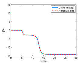
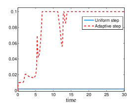
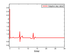
Figure 1: Evolutions of energy (left), time steps (middle) and time steps ratios (right) of the MBE equation using different time strategies until time T=30.

We aim at simulating the benchmark problem with an initial condition of (5.1). We first test the efficiency and accuracy of Algorithm 1. To make a comparison, we shall also show the numerical results with the uniform time meshes. The solution is first simulated until $T=30$ with a constant time step $\tau=10^{-3}$. We then use the adaptive time-stepping strategy described in Algorithm 1 to repeat the simulation. The numerical results are summarized in Figure 1. We note that it takes 30000 uniform time steps with $\tau=10^{-3}$, while the total number of adaptive time steps is only 529 to get the similar results, meaning that the time-stepping adaptive strategy is computationally efficient. In addition, the right subplot in Figure 1 shows that the adaptive step-ratios satisfy the condition S1.

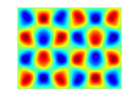
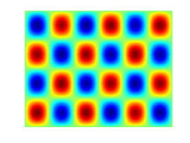
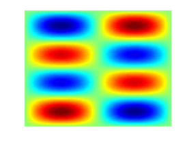
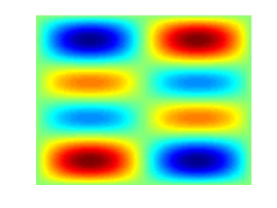
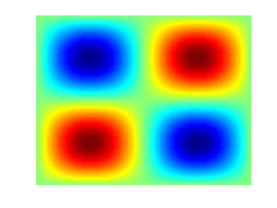
Figure 2: The isolines of numerical solutions of the height function $\phi$ for the MBE equation using adaptive time strategy at $t=0,1,5,10,20,30$, respectively.

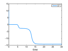
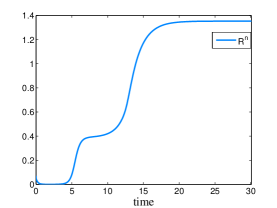
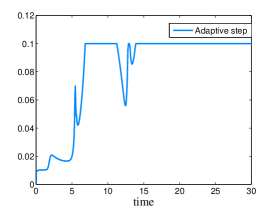
Figure 3: Evolutions of energy (left), roughness (middle) and adaptive time steps (right) for the MBE equation using adaptive time strategy, respectively

The evolutions of the phase variable obtained by adaptive time stepping strategy are depicted in Figure 2 and the evolution of the energy for the MBE model is presented in Figure 2. The discrete energy, roughness, and adaptive time steps are shown in Figure 3. In order to see the numerical performance, we use the same initial data with different parameters $\epsilon=0.2,0.1,0.05$ to carry out the simulations. The energy curves and the correspondingly adaptive steps are summarized in Figure 4. We observe that the variable-step BDF2 scheme (1.7) with the adaptive settings $\tau_{\max}=0.1$ and $\tau_{\min}=10^{-4}$ can work well for the current simulations.

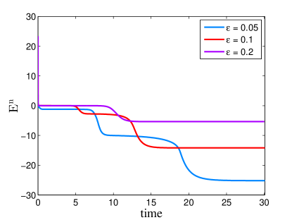
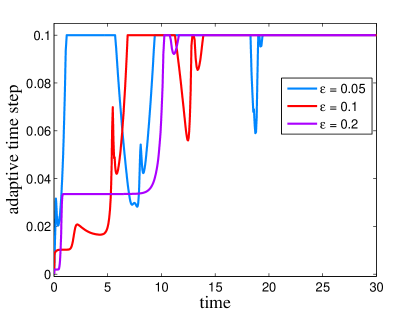
Figure 4: Evolutions of energy (left) and time steps (right) of the MBE equation using initial data (5.1) with different $\varepsilon=0.2,0.1,0.05$ until time T=30.

6 Conclusions

We have performed the stability and convergence analysis of the variable-step BDF2 scheme for the molecular beam epitaxial model without slope selection. The main contribution is that we show that the variable-step BDF2 scheme admits an energy dissipation law under the time-step ratios constraint $r_{k}:=\tau_{k}/\tau_{k-1}<3.561.$ Moreover, the $L^{2}$ norm stability and rigorous error estimates are established under the same step-ratios constraint that ensuring the energy stability., i.e., $0<r_{k}<3.561.$ This is known to be the best result in literature. We remark that the technique in this work is not applicable to molecular beam epitaxial model with slope selection, and we shall pursuit this study in our future works.

References

• [1] J.G. Amar and F. Family, Effects of crystalline microstructure on epitaxial growth, J Phys. Rev., 54 (1996), pp. 14071-14076.
• [2] J. Becker, A second order backward difference method with variable steps for a parabolic problem, BIT, 38(4) (1998), pp. 644–662.
• [3] W. Chen, S. Conde, C. Wang, X. Wang and S. M. Wise, A linear energy stable scheme for a thin film model without slope selection, J Sci. Comput., 52 (2012), pp. 546-562.
• [4] W. Chen, C. Wang and X. Wang, A linear iteration algorithm for a second-order energy stable scheme for a thin film model without slope selection, J Sci. Comput., 59 (2014), pp. 574–601.
• [5] W. Chen, X. Wang, Y. Yan and Z. Zhang, A second order BDF numerical scheme with variable steps for the Cahn–Hilliard equation, SIAM J. Numer. Anal., 57 (1) (2019), pp. 495–525.
• [6] M. Crouzeix and F.J. Lisbona, The convergence of variable-stepsize, variable formula, multistep methods, SIAM J. Numer. Anal., 21 (1984), pp. 512–534.
• [7] E. Emmrich, Stability and error of the variable two-step BDF for semilinear parabolic problems, J. Appl. Math. & Computing, 19 (2005), pp. 33–55.
• [8] J.W. Evans, P.A. Thiel, A little chemistry helps the big get bigger, Science, 330 (2010), pp. 599-600.
• [9] R.D. Grigorieff, Stability of multistep-methods on variable grids, Numer. Math., 42 (1983), pp. 359–377.
• [10] L. Golubovic, Interfacial coarsening in epitaxial growth models without slope selection, Phys. Rev. Lett., 78 (1997), pp. 90-93.
• [11] H. Gomez and T. Hughes, Provably unconditionally stable, second-order time-accurate, mixed variational methods for phase-field models, J. Comput. Phys., 230 (2011), pp.5310–5327.
• [12] L. Ju, X. Li, Z. Qiao and H. Zhang, Energy stability and error estimates of exponential time differencing schemes for the epitaxial growth model without slope selection, Math. Comp., 87 (2018), pp. 1859–1885.
• [13] M.-N. Le Roux, Variable step size multistep methods for parabolic problems, SIAM J. Numer. Anal., 19 (4) (1982), pp. 725–741.
• [14] B. Li and J.G. Liu, Thin film epitaxy with or without slope selection, European J. Appl. Math., 14 (2003), pp. 713–743.
• [15] H.-L. Liao, T. Tang and T. Zhou, On energy stable, maximum-principle preserving, second order BDF scheme with variable steps for the Allen-Cahn equation, SIAM J. Numer. Anal., 2020, to appear.
• [16] H.-L. Liao and Z. Zhang, Analysis of adaptive BDF2 scheme for diffusion equations, Math. Comp., 2020, to appear.
• [17] H.-L Liao, B. Ji and L. Zhang, An adaptive BDF2 implicit time-stepping method for the phase field crystal model, IMA J. Numer. Anal., 2020, in review (arXiv:2008.00212v1).
• [18] Z. Qiao, Z.Z. Sun and Z. Zhang, Stability and convergence of second-order schemes for the nonlinear epitaxial growth model without slope selection, Math Comp., 84 (2015), pp. 653-674.
• [19] Z. Qiao, Z. Zhang and T. Tang, An adaptive time-stepping strategy for the molecular beam epitaxy models, SIAM J. Sci. Comput., 33 (2011), pp. 1395–1414.
• [20] M. Rost and J. Krug, Coarsening of surfaces in unstable epitaxial growth, J Phys. Rev. E., 55 (1997), pp. 4952-3957.
• [21] J. Shen, C. Wang, X. Wang and S.M. Wise, Second-order convex splitting schemes for gradient flows with Ehrlich–Schwoebel type energy: application to thin film epitaxy, SIAM J. Numer. Anal., 50(1) (2012), pp. 105–125.
• [22] J. Xu, Y.K. Li, S.N. Wu and A.Bousequet, On the stability and accuracy of partially and fully implicit schemes for phase field modeling, Comput. Methods Appl. Mech. Engrg., 345 (2019), pp. 826-853.
• [23] C. Xu and T. Tang, Stability analysis of large time-stepping methods for epitaxial growth models, SIAM J. Numer. Anal. 44(4) (2006), pp. 1759–1779.
• [24] Z. Zhang, Y. Ma and Z. Qiao, An adaptive time-stepping strategy for solving the phase field crystal model, J. Comput. Phys., 249 (2013), pp. 204–215.