A note on the asymptotic stability of the Semi-Discrete method for Stochastic Differential Equations

Abstract.

We study the asymptotic stability of the semi-discrete (SD) numerical method for the approximation of stochastic differential equations. Recently, we examined the order of ${\mathcal{L}}^{2}$-convergence of the truncated SD method and showed that it can be arbitrarily close to $1/2,$ see Stamatiou, Halidias (2019), Convergence rates of the Semi-Discrete method for stochastic differential equations, Theory of Stochastic Processes, 24(40). We show that the truncated SD method is able to preserve the asymptotic stability of the underlying SDE. Motivated by a numerical example, we also propose a different SD scheme, using the Lamperti transformation to the original SDE, which we call Lamperti semi-discrete (LSD). Numerical simulations support our theoretical findings.

1. Introduction

We study the following class of scalar stochastic differential equations (SDEs),

(1) $$dx_{t}=a(t,x_{t})dt+b(t,x_{t})dW_{t},\qquad t\in[0,T],$$

where $a,b:[0,T]\times{\mathbb{R}}\rightarrow{\mathbb{R}}$ are measurable functions such that (1) has a unique solution and $x_{0}$ is independent of all $\{W_{t}\}_{t\geq 0}.$ We assume that SDE (1) has non-autonomous coefficients, i.e. $a(t,x),b(t,x)$ depend explicitly on $t.$ SDEs of the type (1) rarely have explicit solutions, therefore the need for numerical approximations for simulations of the solution process $x_{t}(\omega)$ is apparent. In the case of nonlinear drift and diffusion coefficients classical methods may fail to strongly approximate (in the mean-square sense) the solution of (1), c.f. [1], where the Euler method may explode in finite time.

In this direction, we study the semi-discrete (SD) method originally proposed in [2] and further investigated in [3], [4], [5], [6], [7] and recently in [8] and [9]. The main idea behind the semi-discrete method is freezing on each subinterval appropriate parts of the drift and diffusion coefficients of the solution at the beginning of the subinterval so as to obtain explicitly solved SDEs. Of course the way of freezing (discretization) is not unique.

The SD method is a fixed-time step explicit numerical method which strongly converges to the exact solution and also preserves the domain of the solution; if for instance the solution process $x_{t}$ is nonnegative then the approximation process $y_{t}$ is also nonnegative. The ${\mathcal{L}}^{2}$-convergence of the truncated SD method, see [10], was recently shown to be arbitrarily close to $1/2.$

Our main goal is to further examine qualitative properties of the SD method relevant with the stability of the method and answer questions of the following type: Is the SD method able to preserve the asymptotic stability of the underlying SDE?

The answer of the question above is to the positive, and is given in our main result, Theorem 4. In Section 2 we give all the necessary information about the truncated version of the semi-discrete method; the way of construction of the numerical scheme and some useful properties, whereas Section 3 contains the main result with the proof. Section 4 provides a numerical example. Motivated by the SDE appearing in the example, we also propose a different SD scheme, using the Lamperti transformation to the original SDE, which we call Lamperti semi-discrete (LSD). Numerical simulations support our theoretical findings. Finally, Section 5 contains concluding remarks.

2. Setting and Assumptions

Throughout, let $T>0$ and $(\Omega,{\mathcal{F}},\{{\mathcal{F}}_{t}\}_{0\leq t\leq T},{\mathbb{P}})$ be a complete probability space, meaning that the filtration $\{{\mathcal{F}}_{t}\}_{0\leq t\leq T}$ satisfies the usual conditions, i.e. is right continuous and ${\mathcal{F}}_{0}$ includes all ${\mathbb{P}}$-null sets. Let $W_{t,\omega}:[0,T]\times\Omega\rightarrow{\mathbb{R}}$ be a one-dimensional Wiener process adapted to the filtration $\{{\mathcal{F}}_{t}\}_{0\leq t\leq T}.$ Consider SDE (1), which we rewrite here in its integral form

(2) $$x_{t}=x_{0}+\int_{0}^{t}a(s,x_{s})ds+\int_{0}^{t}b(s,x_{s})dW_{s},\quad t\in[0,T],$$

which admits a unique strong solution. In particular, we assume the existence of a predictable stochastic process $x:[0,T]\times\Omega\rightarrow{\mathbb{R}}$ such that ([11, Def. 2.1]),

$$\{a(t,x_{t})\}\in{\mathcal{L}}^{1}([0,T];{\mathbb{R}}),\quad\{b(t,x_{t})\}\in{\mathcal{L}}^{2}([0,T];{\mathbb{R}})$$

and

$${\mathbb{P}}\left[x_{t}=x_{0}+\int_{0}^{t}a(s,x_{s})ds+\int_{0}^{t}b(s,x_{s})dW_{s}\right]=1,\quad\hbox{ for every }t\in[0,T].$$

Assumption 1.

Let $f(s,r,x,y),g(s,r,x,y):[0,T]^{2}\times{\mathbb{R}}^{2}\rightarrow{\mathbb{R}}$ be such that $f(s,s,x,x)=a(s,x),g(s,s,x,x)=b(s,x),$ where $f,g$ satisfy the following condition $(\phi\equiv f,g)$

$$|\phi(s_{1},r_{1},x_{1},y_{1})-\phi(s_{2},r_{2},x_{2},y_{2})|\leq C_{R}\Big{(}|s_{1}-s_{2}|+|r_{1}-r_{2}|+|x_{1}-x_{2}|+|y_{1}-y_{2}|\Big{)}$$

for any $R>0$ such that $|x_{1}|\vee|x_{2}|\vee|y_{1}|\vee|y_{2}|\leq R,$ where the quantity $C_{R}$ depends on $R$ and $x\vee y$ denotes the maximum of $x,y.$

Let us now recall the SD scheme. Consider the equidistant partition $0=t_{0}<t_{1}<...<t_{N}=T$ and $\Delta=T/N.$ We assume that for every $n\leq N-1,$ the following SDE

(3) $$y_{t}=y_{t_{n}}+\int_{t_{n}}^{t}f(t_{n},s,y_{t_{n}},y_{s})ds+\int_{t_{n}}^{t}g(t_{n},s,y_{t_{n}},y_{s})dW_{s},\quad t\in(t_{n},t_{n+1}],$$

with $y_{0}=x_{0}$ a.s., has a unique strong solution.

In order to compare with the exact solution $x_{t},$ which is a continuous time process, we consider the following interpolation process of the semi-discrete approximation, in a compact form,

(4) $$y_{t}=y_{0}+\int_{0}^{t}f(\hat{s},s,y_{\hat{s}},y_{s})ds+\int_{0}^{t}g(\hat{s},s,y_{\hat{s}},y_{s})dW_{s},$$

where $\hat{s}=t_{n}$ when $s\in[t_{n},t_{n+1}).$ Process (4) has jumps at nodes $t_{n}.$ The first and third variable in $f,g$ denote the discretized part of the original SDE. We observe from (4) that in order to solve for $y_{t}$, we have to solve an SDE and not an algebraic equation. The choice $f(s,r,x,y)=a(s,x)$ and $g(s,r,x,y)=b(s,x)$ reproduces the classical Euler scheme.

In the case of superlinear coefficients the numerical scheme (4) converges to the true solution $x_{t}$ of SDE (2) and this is stated in the following, cf. [3],

Theorem 1 (Strong convergence).

Suppose Assumption 1 holds and (3) has a unique strong solution for every $n\leq N-1,$ where $x_{0}\in{\mathcal{L}}^{p}(\Omega,{\mathbb{R}}).$ Let also

$${\mathbb{E}}(\sup_{0\leq t\leq T}|x_{t}|^{p})\vee{\mathbb{E}}(\sup_{0\leq t\leq T}|y_{t}|^{p})<A,$$

for some $p>2$ and $A>0.$ Then the semi-discrete numerical scheme (4) converges to the true solution of (2) in the ${\mathcal{L}}^{2}$-sense, that is

(5) $$\lim_{\Delta\rightarrow 0}{\mathbb{E}}\sup_{0\leq t\leq T}|y_{t}-x_{t}|^{2}=0.$$

Relation (5) does not reveal the order of convergence. We choose a strictly increasing function $\mu:{\mathbb{R}}_{+}\rightarrow{\mathbb{R}}_{+}$ such that for every $s,r\leq T$

(6) $$\sup_{|x|\leq u}\left(|f(s,r,x,y)|\vee|g(s,r,x,y)|\right)\leq\mu(u)(1+|y|),\qquad u\geq 1.$$

The inverse function of $\mu,$ denoted by $\mu^{-1},$ maps $[\mu(1),\infty)$ to ${\mathbb{R}}_{+}.$ Moreover, we choose a strictly decreasing function $h:(0,1]\rightarrow[\mu(1),\infty)$ and a constant $\hat{h}\geq 1\vee\mu(1)$ such that

(7) $$\lim_{\Delta\rightarrow 0}h(\Delta)=\infty\quad\hbox{and}\quad\Delta^{1/6}h(\Delta)\leq\hat{h}\quad\hbox{for every}\quad\Delta\in(0,1].$$

Now, we are ready to define the truncated versions of $f,g.$ Let $\Delta\in(0,1]$ and $f_{\Delta},g_{\Delta}$ defined by

(8) $$\phi_{\Delta}(s,r,x,y):=\phi\left(s,r,(|x|\wedge\mu^{-1}(h(\Delta)))\frac{x}{|x|},y\right),$$

for $x,y\in{\mathbb{R}}$ where we set $x/|x|=0$ when $x=0.$

It follows that the truncated functions $f_{\Delta},g_{\Delta}$ are bounded in the following way for a given step-size $0<\Delta\leq 1,$

(9) $$|f_{\Delta}(s,r,x,y)|\vee|g_{\Delta}(s,r,x,y)| \leq \mu(\mu^{-1}(h(\Delta)))(1+|y|)$$

$$\leq h(\Delta)(1+|y|),$$

for all $x,y\in{\mathbb{R}}.$

For the equidistant partition of $[0,T]$ with $\Delta<1$ consider now the following SDE

(10) $$y_{t}^{\Delta}=y_{t_{n}}^{\Delta}+\int_{t_{n}}^{t}f_{\Delta}(t_{n},s,y_{t_{n}}^{\Delta},y_{s}^{\Delta})ds+\int_{t_{n}}^{t}g_{\Delta}(t_{n},s,y_{t_{n}}^{\Delta},y_{s}^{\Delta})dW_{s},\quad t\in(t_{n},t_{n+1}],$$

with $y_{0}=x_{0}$ a.s. We assume that (10) admits a unique strong solution for every $n\leq N-1$ and rewrite it in compact form,

(11) $$y_{t}^{\Delta}=y_{0}+\int_{0}^{t}f_{\Delta}(\hat{s},s,y_{\hat{s}}^{\Delta},y_{s}^{\Delta})ds+\int_{0}^{t}g_{\Delta}(\hat{s},s,y_{\hat{s}}^{\Delta},y_{s}^{\Delta})dW_{s}.$$

Assumption 2.

Let the truncated versions $f_{\Delta}(s,r,x,y),g_{\Delta}(s,r,x,y)$ of $f,g$ satisfy the following condition $(\phi_{\Delta}\equiv f_{\Delta},g_{\Delta})$

$$|\phi_{\Delta}(s_{1},r_{1},x_{1},y_{1})-\phi_{\Delta}(s_{2},r_{2},x_{2},y_{2})|\leq h(\Delta)\Big{(}|s_{1}-s_{2}|+|r_{1}-r_{2}|+|x_{1}-x_{2}|+|y_{1}-y_{2}|\Big{)}$$

for all $0<\Delta\leq 1$ and $x_{1},x_{2},y_{1},y_{2}\in{\mathbb{R}},$ where $h(\Delta)$ is as in (7).

Let us also assume that the coefficients $a(t,x),b(t,x)$ of the original SDE satisfy the Khasminskii-type condition.

Assumption 3.

We assume the existence of constants $p\geq 2$ and $C_{K}>0$ such that $x_{0}\in{\mathcal{L}}^{p}(\Omega,{\mathbb{R}})$ and

$$xa(t,x)+\frac{p-1}{2}b(t,x)^{2}\leq C_{K}(1+|x|^{2})$$

for all $(t,x)\in[0,T]\times{\mathbb{R}}$.

A well-known result follows (see e.g. [11]) when the SDE (2) satisfies the local Lipschitz condition plus the Khasminskii-type condition.

Lemma 1.

Under Assumptions 1 (for the coefficients $a(t,x),b(t,x)$) and 3 the SDE (2) has a unique global solution and for all $T>0,$ there exists a constant $A>0$ such that

$$\sup_{0\leq t\leq T}{\mathbb{E}}|x_{t}|^{p}<A.$$

Theorem 2 (Order of strong convergence).

Suppose Assumption 2 and Assumption 3 hold and (10) has a unique strong solution for every $n\leq N-1,$ where $x_{0}\in{\mathcal{L}}^{p}(\Omega,{\mathbb{R}})$ for some $p\geq 14+2\gamma.$ Let $\epsilon\in(0,1/3)$ and define for $\gamma>0$

$$\mu(u)=\overline{C}u^{1+\gamma},\quad u\geq 0\quad\hbox{ and }\quad h(\Delta)=\overline{C}+\sqrt{\ln\Delta^{-\epsilon}},\quad\Delta\in(0,1].$$

where $\Delta\leq 1$ and $\hat{h}$ are such that (7) holds. Then the semi-discrete numerical scheme (11) converges to the true solution of (2) in the ${\mathcal{L}}^{2}$-sense with order arbitrarily close to $1/2,$ that is

(12) $${\mathbb{E}}\sup_{0\leq t\leq T}|y^{\Delta}_{t}-x_{t}|^{2}\leq C\Delta^{1-\epsilon}.$$

3. Asymptotic Stability

Now we are ready to study the ability of the truncated SD method to preserve the asymptotic stability of (2). For that reason we also assume that $a(0,0)=0$ and $b(0,0)=0.$ Moreover, to guarantee the asymptotic stability of (2) we use an assumption similar to [12, Assumption 5.1].

Assumption 4.

We assume the existence of a continuous non-decreasing function $\kappa:{\mathbb{R}}_{+}\mapsto{\mathbb{R}}_{+}$ with $\kappa(0)=0$ and $\kappa(u)>0$ for all $u>0$ such that

(13) $$2xa(s,x)+|b(x)|^{2}\leq-\kappa(|x|),$$

for all $x\in{\mathbb{R}}$ and $s\in[0,T].$

Now, we state a result without proof concerning the asymptotic stability of (2), see also [12, Theorem 5.2] where autonomous coefficients are assumed.

Theorem 3 (asymptotic stability of underlying process).

Let Assumption 4 hold. Then the solution process of SDE (2) is asymptotically stable, that is

(14) $$\lim_{t\to\infty}x_{t}=0\hbox{ a.s.}$$

for any $x_{0}\in{\mathbb{R}}.$

Recall equation (10) which defines the truncated SD numerical scheme. We rewrite our proposed scheme, that is the solution of (10) at the discrete points $0,t_{1},\ldots,t_{n+1},$ in the following way

(15) $$y_{n+1}^{\Delta}=\phi^{\Delta}(y_{n}^{\Delta},t_{n},\Delta,\Delta W_{n}),$$

where $\Delta W_{n}$ are the Wiener increments, $\Delta=t_{n+1}-t_{n}$ is the step-size and $y_{n}$ stands for $y_{t_{n}}.$ We assume the following decomposition of $\phi^{\Delta}(y_{n}^{\Delta},t_{n},\Delta,\Delta W_{n})$ for the above representation (15),

(16) $$\phi^{\Delta}(y_{n}^{\Delta},t_{n},\Delta,\Delta W_{n})^{2}=(y_{n}^{\Delta})^{2}+\phi_{1}^{\Delta}(y_{n}^{\Delta},t_{n},\Delta)+\phi_{2}^{\Delta}(y_{n}^{\Delta},t_{n},\Delta,\Delta W_{n}),$$

where ${\mathbb{E}}(\phi_{2}^{\Delta}(y_{n}^{\Delta},t_{n},\Delta,\Delta W_{n})|{\mathcal{F}}_{t_{n}})=0.$ The following theorem shows that the truncated SD method is able to preserve the asymptotic stability property of the underlying SDE.

Theorem 4 (asymptotic numeric stability).

Let the auxiliary function $\phi_{1}^{\Delta}$ from (16) satisfy

(17) $$\phi_{1}^{\Delta}(y_{n}^{\Delta},t_{n},\Delta)\leq-\kappa_{1}\left(\left|(|y_{n}^{\Delta}|\wedge\mu^{-1}(h(\Delta)))\frac{y_{n}^{\Delta}}{|y_{n}^{\Delta}|}\right|\right),$$

for any $0<\Delta\leq\Delta^{*},$ where $\kappa_{1}$ has the same properties as $\kappa$ in (13) with $\kappa_{1}\leq\kappa$. Let also Assumption 4 hold.

Then the solution of the truncated SD method (15) is numerically asymptotically stable, that is

(18) $$\lim_{n\to\infty}y_{n}^{\Delta}=0\hbox{ a.s.}$$

for all $x_{0}\in{\mathbb{R}}$ and $0<\Delta\leq\Delta^{*}$.

Proof of Theorem 4.

Let us first fix a $\Delta\in(0,\Delta^{*}].$ Denote

$$\pi_{\Delta}(x):=\left(|x|\wedge\mu^{-1}(h(\Delta))\right)\frac{x}{|x|}.$$

Then combining (15), (16) and (17) we get

$$(y_{n+1}^{\Delta})^{2} \leq (y_{n}^{\Delta})^{2}-\kappa_{1}\left(\left|\pi_{\Delta}(y_{n}^{\Delta})\right|\right)+\phi_{2}^{\Delta}(y_{n}^{\Delta},t_{n},\Delta,\Delta W_{n})$$

$$\leq (x_{0})^{2}-\sum_{j=0}^{n}\kappa_{1}\left(\left|\pi_{\Delta}(y_{j}^{\Delta})\right|\right)+M_{n},$$

where $M_{n}:=\sum_{j=0}^{n}\phi_{2}^{\Delta}(y_{j}^{\Delta},t_{j},\Delta,\Delta W_{j}).$ Recalling that ${\mathbb{E}}(\phi_{2}^{\Delta}(y_{n}^{\Delta},t_{n},\Delta,\Delta W_{n})|{\mathcal{F}}_{t_{n}})=0$ implies that $M_{n},n=0,1,\ldots,$ is a martingale. Application of the nonnegative semi-martingale convergence theorem, c.f. [13, Theorem 7, p.139], implies

$$\sum_{j=0}^{\infty}\kappa_{1}\left(\left|\pi_{\Delta}(y_{j}^{\Delta})\right|\right)<\infty\hbox{ a.s.}$$

which in turn

$$\lim_{j\rightarrow\infty}\kappa_{1}\left(\left|\pi_{\Delta}(y_{j}^{\Delta})\right|\right)=0\hbox{ a.s.}$$

By the property of the function $\kappa_{1}$ we get that

$$\lim_{j\rightarrow\infty}\left(|y_{j}^{\Delta}|\wedge\mu^{-1}(h(\Delta))\right)\frac{y_{j}^{\Delta}}{|y_{j}^{\Delta}|}=0\hbox{ a.s.}$$

Assertion (18) follows. ∎

4. Example

We will use the numerical example of [12, Example 5.4], that is we consider an autonomous SDE of the form (2) with $a(x)=-10x^{3}$ and $b(x)=x^{2},$ with initial condition $x_{0}\in{\mathbb{R}}$, that is,

(19) $$x_{t}=x_{0}-10\int_{0}^{t}x_{s}^{3}ds+\int_{0}^{t}x_{s}^{2}dW_{s},\qquad t\geq 0.$$

Using standard arguments one may show that the solution process of SDE (19) is positive, see Appendix B. Assumption 4 holds with $\kappa(u)=19u^{4}$ therefore by Theorem 3 SDE (19) is almost surely asymptotically stable. The classical Euler Maruyama method is not able to reproduce this asymptotic stability, see [12, Appendix]. In the following we show that the truncated SD method can reproduce this asymptotic stability. Since, in the construction of the semi discrete method the way of discretizing is not unique (but rather indicated by the equation itself) we will try two versions of the SD method by freezing different parts of the diffusion coefficient. We first choose the auxiliary functions $f,g_{1}$ and $g_{2}$ in the following way

$$f(s,r,x,y)=-10x^{2}y,\qquad g_{1}(s,r,x,y)=x,\qquad g_{2}(s,r,x,y)=x^{2},$$

thus (3) becomes

(20) $$y_{t}=y_{t_{n}}-10y_{t_{n}}^{2}\int_{t_{n}}^{t}y_{s}ds+y_{t_{n}}^{2}\int_{t_{n}}^{t}dW_{s},\quad t\in(t_{n},t_{n+1}],$$

and

(21) $$\hat{y}_{t}=\hat{y}_{t_{n}}-10\hat{y}_{t_{n}}^{2}\int_{t_{n}}^{t}\hat{y}_{s}ds+\hat{y}_{t_{n}}\int_{t_{n}}^{t}\hat{y}_{s}dW_{s},\quad t\in(t_{n},t_{n+1}],$$

respectively, with $y_{0}=\hat{y}_{0}=x_{0}$ a.s. SDEs (20) and (21) are linear equations ( (20) is linear in the narrow sense and is known as Langevin equation) with variable coefficients which admit a unique strong solution, c.f. [14, Chapter 4.4] and Appendix A. In particular,

(22) $$y_{n+1}=e^{-10y_{n}^{2}\Delta}\left(y_{n}+y_{n}^{2}\int_{t_{n}}^{t_{n+1}}e^{10y_{n}^{2}(s-t_{n})}dW_{s}\right),\quad n\in{\mathbb{N}},$$

and

(23) $$\hat{y}_{n+1}=\hat{y}_{n}\exp\left\{-\frac{21}{2}\hat{y}_{n}^{2}\Delta+\hat{y}_{n}\Delta W_{n}\right\},\quad n\in{\mathbb{N}}.$$

Note that (6) holds with $\mu(u)=10|u|^{2}$ since

$$\sup_{|x|\leq u}\left(|-10x^{2}y|\vee|x|\vee|x^{2}|\right)\leq 10|u|^{2}(1+|y|),\qquad u\geq 1.$$

Therefore, in the notation of Theorem 2, $\gamma=1$ and $\overline{C}=10.$ Finally, $h(\Delta)=10+\sqrt{\ln\Delta^{-\epsilon_{1}}}$ for any $\Delta\in(0,1].$ Clearly $h(1)\geq\mu(1)$ and

$$\Delta^{1/6}h(\Delta)\leq 10\Delta^{1/6}+\sqrt{\Delta^{1/3}\ln\Delta^{-\epsilon_{1}}}\leq 11,$$

for any $\Delta\in(0,1]$ and $0<\epsilon_{1}\leq 1/3.$ Therefore we take $\hat{h}=11.$ The truncated versions of the semi-discrete method (TSD) read,

(24) $$y_{n+1}^{\Delta}=e^{-10\pi^{2}_{\Delta}(y_{n}^{\Delta})\Delta}\left(y_{n}^{\Delta}+\pi^{2}_{\Delta}(y_{n}^{\Delta})\int_{t_{n}}^{t_{n+1}}e^{10\pi^{2}_{\Delta}(y_{n}^{\Delta})(s-t_{n})}dW_{s}\right)$$

and

(25) $$\hat{y}_{n+1}^{\Delta}=\hat{y}_{n}^{\Delta}\exp\left\{-\frac{21}{2}\pi^{2}_{\Delta}(\hat{y}_{n}^{\Delta})\Delta+\pi_{\Delta}(\hat{y}_{n}^{\Delta})\Delta W_{n}\right\}$$

for $n\in{\mathbb{N}},$ where

$$\pi_{\Delta}(x)=\left(|x|\wedge\sqrt{\frac{h(\Delta)}{10}}\right)\frac{x}{|x|}$$

and therefore

$$\pi^{2}_{\Delta}(x)=|x|^{2}\wedge\frac{h(\Delta)}{10}.$$

4.1. Asymptotic stability of truncated Semi-Discrete method

Now, we compute $(y_{n+1}^{\Delta})^{2}$ taking the square of (24) and making some rearrangements to show that it admits representation (16).

$$(y_{n+1}^{\Delta})^{2}=(y_{n}^{\Delta})^{2}e^{-20\pi^{2}_{\Delta}(y_{n}^{\Delta})\Delta}+2y_{n}^{\Delta}e^{-10\pi^{2}_{\Delta}(y_{n}^{\Delta})t_{n+1}}\pi^{2}_{\Delta}(y_{n}^{\Delta})\int_{t_{n}}^{t_{n+1}}e^{10\pi^{2}_{\Delta}(y_{n}^{\Delta})s}dW_{s}$$

$$+\pi^{4}_{\Delta}(y_{n}^{\Delta})e^{-20\pi^{2}_{\Delta}(y_{n}^{\Delta})t_{n+1}}\left(\int_{t_{n}}^{t_{n+1}}e^{10\pi^{2}_{\Delta}(y_{n}^{\Delta})s}dW_{s}\right)^{2}$$

$$= (y_{n}^{\Delta})^{2}-(1-e^{-20\pi^{2}_{\Delta}(y_{n}^{\Delta})t_{n+1}})(y_{n}^{\Delta})^{2}+\frac{1}{20}\pi^{2}_{\Delta}(y_{n}^{\Delta})e^{-20\pi^{2}_{\Delta}(y_{n}^{\Delta})t_{n+1}}(e^{20\pi^{2}_{\Delta}(y_{n}^{\Delta})t_{n+1}}-e^{20\pi^{2}_{\Delta}(y_{n}^{\Delta})t_{n}})$$

$$+2y_{n}^{\Delta}e^{-10\pi^{2}_{\Delta}(y_{n}^{\Delta})t_{n+1}}\pi^{2}_{\Delta}(y_{n}^{\Delta})\int_{t_{n}}^{t_{n+1}}e^{10\pi^{2}_{\Delta}(y_{n}^{\Delta})s}dW_{s}$$

$$+\pi^{4}_{\Delta}(y_{n}^{\Delta})e^{-20\pi^{2}_{\Delta}(y_{n}^{\Delta})t_{n+1}}\left(\int_{t_{n}}^{t_{n+1}}e^{10\pi^{2}_{\Delta}(y_{n}^{\Delta})s}dW_{s}\right)^{2}$$

$$-\frac{1}{20}\pi^{2}_{\Delta}(y_{n}^{\Delta})e^{-20\pi^{2}_{\Delta}(y_{n}^{\Delta})t_{n+1}}(e^{20\pi^{2}_{\Delta}(y_{n}^{\Delta})t_{n+1}}-e^{20\pi^{2}_{\Delta}(y_{n}^{\Delta})t_{n}}).$$

Denote $I:=I(y_{n}^{\Delta},t_{n},\Delta,\Delta W_{n})=\int_{t_{n}}^{t_{n+1}}e^{10\pi^{2}_{\Delta}(y_{n}^{\Delta})s}dW_{s}$ and set

$$\phi_{2}^{\Delta}(y_{n}^{\Delta},t_{n},\Delta,\Delta W_{n}) := 2y_{n}^{\Delta}e^{-10\pi^{2}_{\Delta}(y_{n}^{\Delta})t_{n+1}}\pi^{2}_{\Delta}(y_{n}^{\Delta})I+\pi^{4}_{\Delta}(y_{n}^{\Delta})e^{-20\pi^{2}_{\Delta}(y_{n}^{\Delta})t_{n+1}}I^{2}$$

$$-\frac{1}{20}\pi^{2}_{\Delta}(y_{n}^{\Delta})e^{-20\pi^{2}_{\Delta}(y_{n}^{\Delta})t_{n+1}}(e^{20\pi^{2}_{\Delta}(y_{n}^{\Delta})t_{n+1}}-e^{20\pi^{2}_{\Delta}(y_{n}^{\Delta})t_{n}})$$

to see that ${\mathbb{E}}(\phi_{2}^{\Delta}(y_{n}^{\Delta},t_{n},\Delta,\Delta W_{n})|{\mathcal{F}}_{t_{n}})=0.$ Moreover

$$\phi_{1}^{\Delta}(y_{n}^{\Delta},t_{n},\Delta) := -(1-e^{-20\pi^{2}_{\Delta}(y_{n}^{\Delta})\Delta})(y_{n}^{\Delta})^{2}+\frac{1}{20}\pi^{2}_{\Delta}(y_{n}^{\Delta})(1-e^{-20\pi^{2}_{\Delta}(y_{n}^{\Delta})\Delta})$$

$$\leq -\frac{19}{20}\left(1-e^{-20\pi^{2}_{\Delta}(y_{n}^{\Delta})\Delta}\right)\pi^{2}_{\Delta}(y_{n}^{\Delta}),$$

implying that we may choose $\kappa_{1}$ in the following way

$$\kappa_{1}(u):=-\frac{19}{20}(1-e^{-20u^{2}\Delta})u^{2},$$

so that condition (17) holds and therefore Theorem 4 applies. Note that $\kappa_{1}(0)=0$ and $\kappa_{1}(u)>0$ for any $\Delta>0.$ We conclude that the truncated SD scheme (24) preserves the asymptotic stability perfectly in the sense that $\lim_{n\to\infty}y_{n}^{\Delta}=0$ a.s. for any $0<\Delta\leq 1.$

4.2. Asymptotic stability of exponential truncated Semi-Discrete method

We examine $(\hat{y}_{n+1}^{\Delta})^{2}.$ We take the square of (25) and get that

$$(\hat{y}_{n+1}^{\Delta})^{2}=(\hat{y}_{n}^{\Delta})^{2}e^{-21\pi^{2}_{\Delta}(\hat{y}_{n}^{\Delta})\Delta+2\pi_{\Delta}(\hat{y}_{n}^{\Delta})\Delta W_{n}}$$

$$= (\hat{y}_{n}^{\Delta})^{2}-(1-e^{-19\pi^{2}_{\Delta}(\hat{y}_{n}^{\Delta})\Delta})(\hat{y}_{n}^{\Delta})^{2}+(\hat{y}_{n}^{\Delta})^{2}e^{-19\pi^{2}_{\Delta}(\hat{y}_{n}^{\Delta})\Delta}(1-e^{-2\pi^{2}_{\Delta}(\hat{y}_{n}^{\Delta})\Delta+2\pi_{\Delta}(\hat{y}_{n}^{\Delta})\Delta W_{n}}).$$

Set the last term of the above equality to $\phi_{2}^{\Delta},$ that is

$$\phi_{2}^{\Delta}(\hat{y}_{n}^{\Delta},t_{n},\Delta,\Delta W_{n}):=(\hat{y}_{n}^{\Delta})^{2}e^{-19\pi^{2}_{\Delta}(\hat{y}_{n}^{\Delta})\Delta}(1-e^{-2\pi^{2}_{\Delta}(\hat{y}_{n}^{\Delta})\Delta+2\pi_{\Delta}(\hat{y}_{n}^{\Delta})\Delta W_{n}})$$

to see that ${\mathbb{E}}(\phi_{2}^{\Delta}(y_{n}^{\Delta},t_{n},\Delta,\Delta W_{n})|{\mathcal{F}}_{t_{n}})=0$ since ${\mathcal{E}}_{n}:=e^{-2\pi^{2}_{\Delta}(\hat{y}_{n}^{\Delta})\Delta+2\pi_{\Delta}(\hat{y}_{n}^{\Delta})\Delta W_{n}}$ is an exponential martingale.

Moreover

$$\phi_{1}^{\Delta}(\hat{y}_{n}^{\Delta},t_{n},\Delta) := -(1-e^{-19\pi^{2}_{\Delta}(\hat{y}_{n}^{\Delta})\Delta})(\hat{y}_{n}^{\Delta})^{2}$$

$$\leq -\left(1-e^{-19\pi^{2}_{\Delta}(\hat{y}_{n}^{\Delta})\Delta}\right)\pi^{2}_{\Delta}(\hat{y}_{n}^{\Delta}),$$

implying that we may choose $\kappa_{1}$ in the following way

$$\kappa_{1}(u):=-(1-e^{-19u^{2}\Delta})u^{2},$$

so that once more condition (17) holds and consequently Theorem 4 applies. We conclude that the truncated exponential SD scheme (25) preserves the asymptotic stability perfectly in the sense that $\lim_{n\to\infty}\hat{y}_{n}^{\Delta}=0$ a.s. for any $0<\Delta\leq 1.$

4.3. Semi-Discrete method and Lampreti transformation

Instead of approximating directly (19) we first study a transformation of it, which produces a new SDE with constant diffusion coefficient; in other words we use the Lamperti transformation of (19). In particular, consider $z=-1/x.$ The Itô formula implies the following dynamics for $(z_{t}),$ see Appendix C,

(26) $$z_{t}=z_{0}+11\int_{0}^{t}(z_{s})^{-1}ds+\int_{0}^{t}dW_{s},\qquad t\geq 0.$$

Let $t\in(t_{n},t_{n+1}]$ and

(27) $$\widetilde{y}_{t}=\Delta W_{n}+\widetilde{y}_{t_{n}}+11\int_{t_{n}}^{t}(\widetilde{y}_{s})^{-1}ds,$$

with $\widetilde{y}_{0}=z_{0}.$ (27) is a Bernoulli type equation with solution satisfying

(28) $$(\widetilde{y}_{t})^{2}=(\Delta W_{n}+\widetilde{y}_{t_{n}})^{2}+22(t-t_{n}).$$

Recall that when $x_{0}>0,$ the solution process $x_{t}>0$ a.s. which implies $z_{t}<0$ a.s. which in turn suggests that we take the negative root of (28) as the solution Therefore we propose the following semi-discrete method for the approximation of (26),

(29) $$\widetilde{y}_{t_{n+1}}=-\sqrt{(\Delta W_{n}+\widetilde{y}_{t_{n}})^{2}+22\Delta},$$

which suggests the Lamperti semi-discrete method $(\widetilde{z}_{n})_{n\in{\mathbb{N}}}$ for the approximation of (19)

(30) $$\widetilde{z}_{t_{n+1}}=\frac{1}{\sqrt{(\Delta W_{n}+\widetilde{y}_{t_{n}})^{2}+22\Delta}}.$$

4.4. Simulation Paths

We present simulations for the numerical approximation of (19) with $x_{0}=10$ and compare with the truncated Euler Maruyama method (TEM), which reads

(31) $$y_{n+1}^{TEM}=y_{n}-10\left(|y_{n}|\wedge\bar{\mu}^{-1}(\bar{h}(\Delta))\frac{y_{n}}{|y_{n}|}\right)^{3}\Delta+\left(|y_{n}|\wedge\bar{\mu}^{-1}(\bar{h}(\Delta))\right)^{2}\Delta W_{n},$$

for $n\in{\mathbb{N}},$ where $\bar{h}(\Delta)=\Delta^{-1/4},\bar{\mu}(u)=10u^{3}.$ According to the results in [12] it is shown that method (31) is asymptotically stable for any $\Delta\leq 0.095,$ therefore for such small step sizes we compare all the methods presented here and for bigger $\Delta$ only the SD schemes (22), (23), (24) and (25). We also present the Lamperti semi-discrete scheme (LSD) (30). Moreover, the TEM method does not preserve positivity. Figures 1, 2 and 3 shows sample simulations paths of TSD and TEM respectively for various stepsizes. Note that the truncated TSD, exponential truncated expTSD and the Lamperti LSD works for all $\Delta<1.$

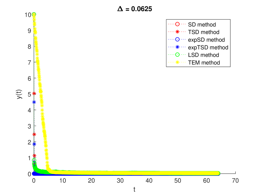
(a) Trajectory for (22) - (25), (30) and (31).

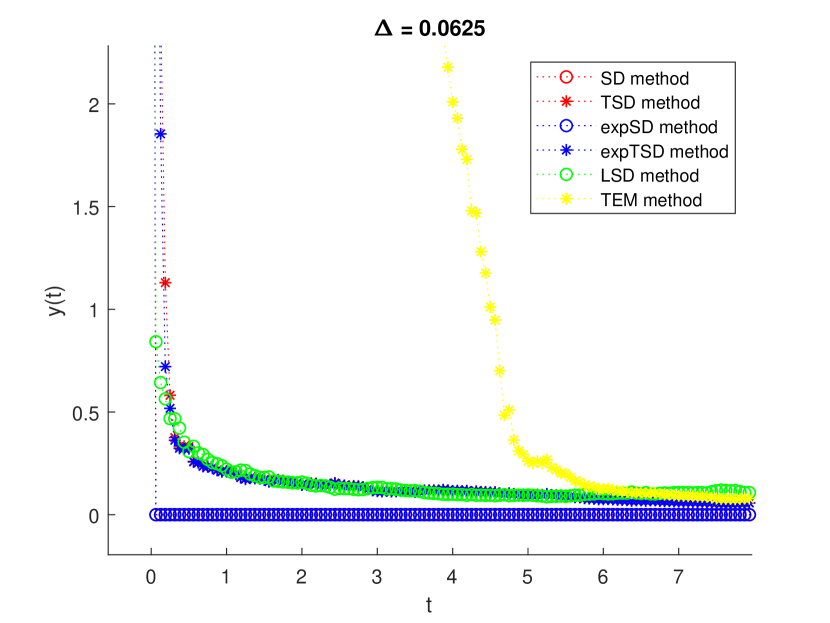
(b) Zoom of Figure 1(A).

Figure 1. Trajectories of (22) -(31), (30) and (31) for the approximation of (19) with $\Delta<0.095$.

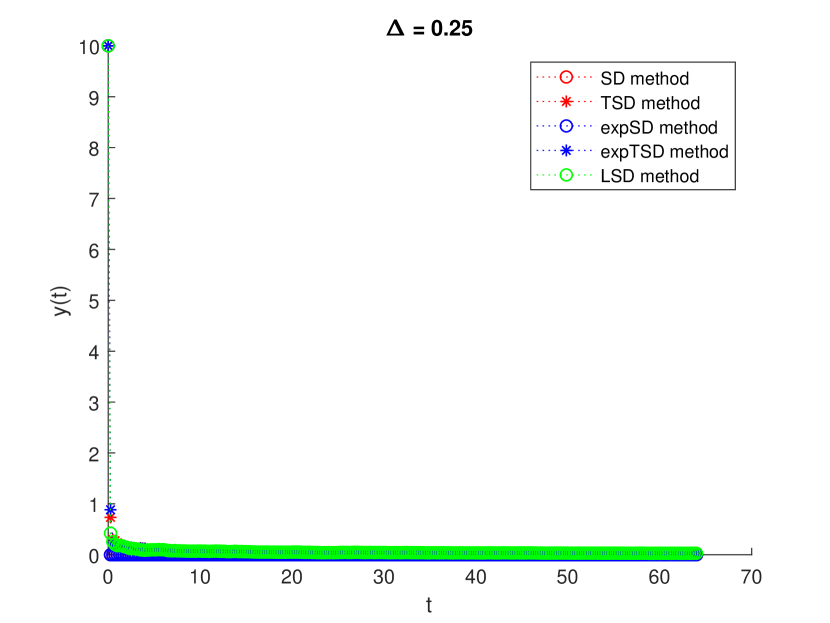
(a) Trajectory for (22) -(25) and (30).

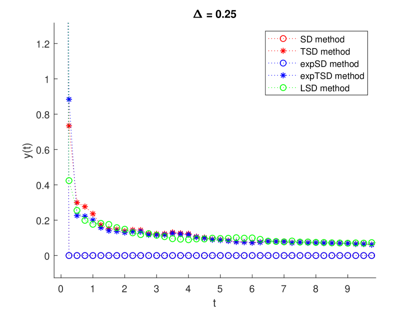
(b) Zoom of Figure 2(A).

Figure 2. Trajectories of (22) -(25) and (30) for the approximation of (19) with $\Delta=0.25$.

In the numerical simulation of the stochastic integral of the (truncated) TSD methods (22) and (24) we used the approximation $\int_{t_{n}}^{t_{n+1}}e^{10\pi^{2}_{\Delta}(y_{n}^{\Delta})s}dW_{s}\approx e^{10\pi^{2}_{\Delta}(y_{n}^{\Delta})t_{n}}\Delta W_{n},$ that is we calculated the integrand in the lower limit of integration. The above equality is of the order $\Delta^{r},$ with $0<r<1/2,$ see Appendix D.

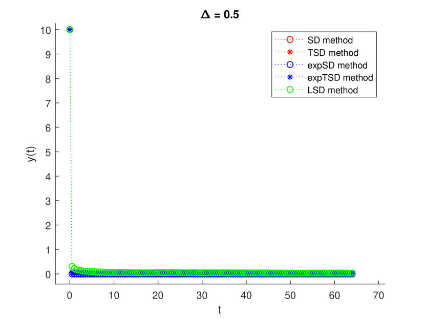
(a) Trajectory for (22) -(25) and (30).

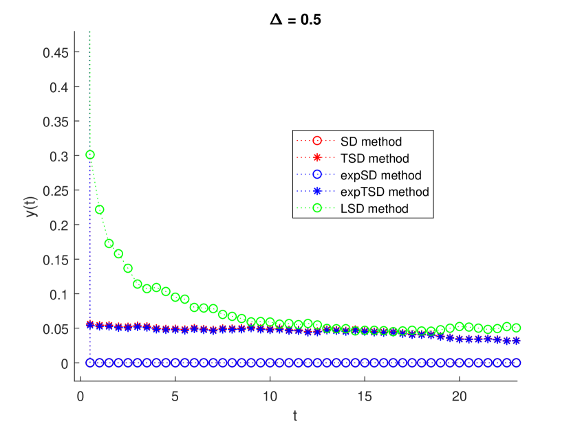
(b) Zoom of Figure 3(A).

Figure 3. Trajectories of (22) - (25) and (30) for the approximation of (19) with $\Delta=0.5$.

We also present in Figure 4 the difference between the Lamperti semi-discrete and the truncated Euler-Maryauma scheme, $y_{TEM}-y_{TSD}$ for small enough $\Delta$ such that $TSD$ works.

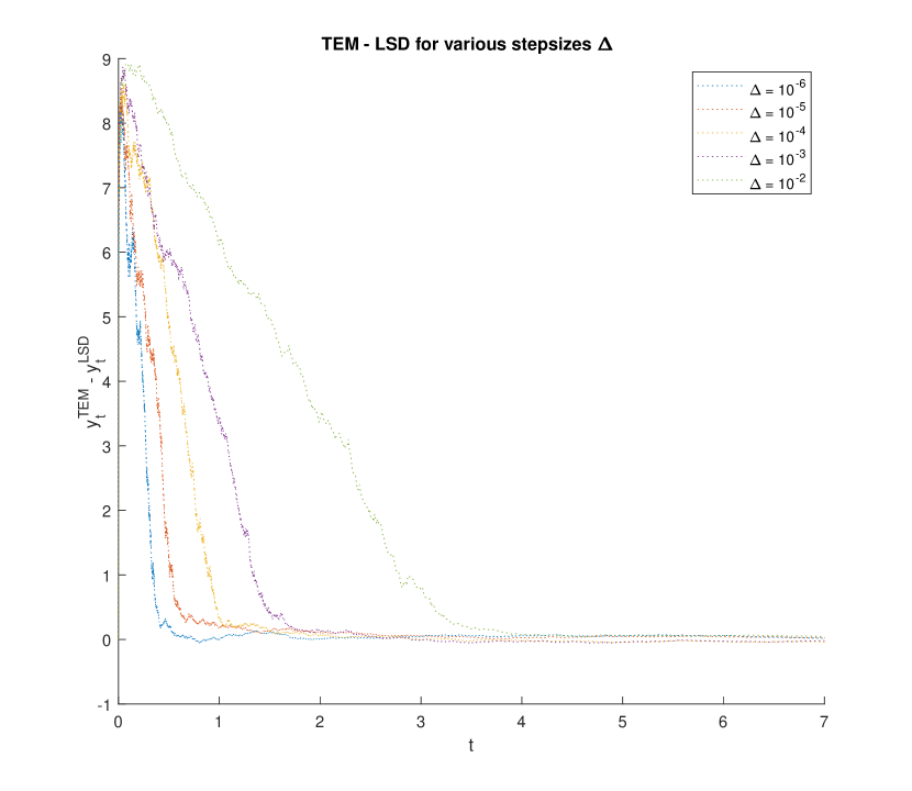
Figure 4. Difference of (31) - (30) for the approximation of (19) with various step sizes.

5. Conclusion and Future Work

In this paper we study the asymptotic stability of the semi-discrete (SD) numerical method for the approximation of stochastic differential equations. Recently, we examined the order of ${\mathcal{L}}^{2}$-convergence of the truncated SD method and showed that it can be arbitrarily close to $1/2,$ see [10]. We show that the truncated SD method is able to preserve the asymptotic stability of the underlying SDE. Motivated by a numerical example, we also propose a different SD scheme, where we actually approximate first the Lamperti transformation of the original SDE. We call this scheme Lamperti semi-discrete (LSD). It preserves positivity (in this case) of the solution, has similar asymptotic properties as the other versions of the SD method and seems promising, since there is no need for an exponential calculation. We will study the LSD method, and its properties in a forthcoming paper.

Appendix A Solution of linear SDEs in the narrow sense

Consider the following linear in the narrow sense SDE,

(32) $$x_{t}=x_{t_{0}}+\int_{t_{0}}^{t}ax_{s}ds+\int_{t_{0}}^{t}bdW_{s},$$

for $t\geq t_{0},$ where $a,b$ are constants. Applying the Itô formula to the transformation $U(t,x)=e^{-a(t-t_{0})}x$, we obtain

$$dU(t,x) = \left(\frac{de^{-a(t-t_{0})}}{dt}x_{t}+ax_{t}e^{-a(t-t_{0})}\right)dt+be^{-a(t-t_{0})}dW_{t}$$

$$= be^{-a(t-t_{0})}dW_{t},$$

or

$$e^{-a(t-t_{0})}x_{t} = x_{t_{0}}+b\int_{t_{0}}^{t}e^{-a(s-t_{0})}dW_{s}$$

$$x_{t} = e^{a(t-t_{0})}x_{t_{0}}+be^{a(t-t_{0})}\int_{t_{0}}^{t}e^{-a(s-t_{0})}dW_{s}.$$

Appendix B Positivity of (19)

In order to prove that $x_{t}>0$ a.s. we first show moment bounds of the SDE (19).

Lemma 2 (Uniform moment bounds for $(x_{t})$).

The solution process $(x_{t})$ of SDE (19) satisfies

$${\mathbb{E}}(\sup_{0\leq t\leq T}(x_{t})^{p})<A,$$

for some $A>0$ and any integer $p$ with $2\leq p\leq 19/2.$

Proof of Lemma 2.

For all $|x|>R$ with $R>1,$ we have that

$$J(x) := \frac{xa(x)+(p-1)b^{2}(x)/2}{1+x^{2}}=\frac{x(-10x^{3})+(p-1)x^{4}/2}{1+x^{2}}$$

$$= \frac{-21+p}{2}\frac{x^{4}}{1+x^{2}}\leq 0,$$

where the last inequality is valid for all $p$ such that $p\leq 21.$ Thus $J(x)$ is bounded for all $x\in{\mathbb{R}},$ since when $|x|\leq R.$ Application of [11, Th. 2.4.1] implies

$${\mathbb{E}}(x_{t})^{p}\leq 2^{(p-2)/2}(1+(x_{0})^{p}),$$

for any $2\leq p\leq 21,$ since $x_{0}\in{\mathbb{R}}.$ Using Itô’s formula on $(x_{t})^{p},$ with $p\leq 19/2$ (in order to use Doob’s martingale inequality later) we have that

$$(x_{t})^{p} = (x_{0})^{p}+\int_{0}^{t}\left(p(x_{s})^{p-1}(-10x_{s}^{3})+\frac{p(p-1)}{2}(x_{s})^{p-2}x_{s}^{4}\right)ds$$

$$+\int_{0}^{t}p(x_{s})^{p-1}x_{s}^{2}dW_{s}$$

$$\leq (x_{0})^{p}+p\int_{0}^{t}(-10+\frac{p-1}{2})(x_{s})^{p+2}ds+M_{t}$$

$$\leq (x_{0})^{p}+M_{t},$$

for any even $p$ with $2\leq p\leq 21,$ or $p=21,$ where $M_{t}=\int_{0}^{t}p(x_{s})^{p+1}dW_{s}.$ Taking the supremum and then expectations in the above inequality we get

$${\mathbb{E}}(\sup_{0\leq t\leq T}(x_{t})^{p}) \leq {\mathbb{E}}(x_{0})^{p}+{\mathbb{E}}\sup_{0\leq t\leq T}M_{t}$$

$$\leq (x_{0})^{p}+\sqrt{{\mathbb{E}}\sup_{0\leq t\leq T}M_{t}^{2}}$$

$$\leq (x_{0})^{p}+\sqrt{4{\mathbb{E}}M_{T}^{2}},$$

where in the last step we have used Doob’s martingale inequality to the diffusion term $M_{t}.$ ∎

Lemma 3 (Positivity of $(x_{t})$).

The solution process $(x_{t})$ of SDE (19) is positive in the sense that $x_{t}>0$ a.s.

Proof of Lemma 3.

Set the stopping time $\theta_{R}=\inf\{t\in[0,T]:x_{t}^{-1}>R\},$ for some $R>0,$ with the convention that $\inf\emptyset=\infty.$ Application of Itô’s formula on $(x_{t\wedge\theta_{R}})^{-2}$ implies,

$$(x_{t\wedge\theta_{R}})^{-2}=(x_{0})^{-2}+\int_{0}^{t\wedge\theta_{R}}(-2)\left((x_{s})^{-3}(-10)(x_{s})^{3}+3(x_{s})^{-4}(x_{s})^{4}\right)ds$$

$$+\int_{0}^{t\wedge\theta_{R}}(-2)(x_{s})^{-3}x_{s}^{2}dW_{s}$$

$$\leq (x_{0})^{-2}+\int_{0}^{t\wedge\theta_{R}}23ds+\int_{0}^{t}(-2)x_{s}^{-1}dW_{s}$$

$$\leq (x_{0})^{-2}+23T+M_{t},$$

where $M_{t}:=\int_{0}^{t}(-2)x_{s}^{-1}{\mathbb{I}}_{(0,t\wedge\theta_{R})}(s)dW_{s}.$ Taking expectations in the above inequality and using the fact that ${\mathbb{E}}M_{t}=0,$ we get that

$${\mathbb{E}}(x_{t\wedge\theta_{R}})^{-2}\leq(x_{0})^{-2}+23T<C,$$

with $C$ independent of $R.$ Therefore

$${\mathbb{E}}\left(\frac{1}{x_{t\wedge\theta_{R}}^{2}}\right)=R^{2}{\mathbb{P}}(\theta_{R}\leq t)+{\mathbb{E}}\left(\frac{1}{x_{t}^{2}}{\mathbb{I}}_{(t<\theta_{R})}\right)<C,$$

implying that

$${\mathbb{P}}(x_{t}\leq 0)={\mathbb{P}}\left(\bigcap_{R=1}^{\infty}\Big{\{}x_{t}<\frac{1}{R}\Big{\}}\right)=\lim_{R\to\infty}{\mathbb{P}}\left(\Big{\{}x_{t}<\frac{1}{R}\Big{\}}\right)\leq\lim_{R\to\infty}{\mathbb{P}}(\theta_{R}\leq t)=0.$$

We conclude that $x_{t}>0$ a.s. ∎

Appendix C Lamperti Tranformation of (19)

Applying the Itô formula to the transformation $z(x)=-1/x,$ we obtain

$$dz_{t} = \left((x_{t})^{-2}(-10)(x_{t})^{3}+\frac{1}{2}(-2)(x_{t})^{-3}(x_{t})^{4}\right)dt+(x_{t})^{-2}(x_{t})^{2}dW_{t}$$

$$= -11x_{t}+dW_{t}$$

$$= 11(z_{t})^{-1}dt+dW_{t}$$

or for $t\geq t_{0}$

$$z_{t} = z_{t_{0}}+11\int_{t_{0}}^{t}(z_{s})^{-1}+\int_{t_{0}}^{t}dW_{s}$$

$$= z_{t_{0}}+11\int_{t_{0}}^{t}(z_{s})^{-1}+W_{t}-W_{t_{0}}.$$

Appendix D Stochastic Integral Approximation

We want to estimate the stochastic integral appearing in the proposed truncated semi-discrete method (24) for the approximation of SDE (19). In a similar way we calculate the integral appearing in the exponential truncated semi-discrete scheme (22).

In the numerical simulations we used the following relation

$$\int_{t_{n}}^{t_{n+1}}e^{10\pi^{2}_{\Delta}(y_{n}^{\Delta})s}dW_{s}\approx e^{10\pi^{2}_{\Delta}(y_{n}^{\Delta})t_{n}}\Delta W_{n}.$$

We show the following estimation

(33) $${\mathbb{P}}\left(\left|\int_{t_{n}}^{t_{n+1}}e^{10\pi^{2}_{\Delta}(y_{n}^{\Delta})s}dW_{s}-e^{10\pi^{2}_{\Delta}(y_{n}^{\Delta})t_{n}}\Delta W_{n}\right|\geq\Delta^{r}\right)\leq 2e^{20\pi^{2}_{\Delta}(y_{n}^{\Delta})t_{n+1}}\Delta^{1-2r},$$

suggesting that the probability of the absolute difference of these two random variables being of order $\Delta^{r},$ with $0<r<1/2,$ approaches unity as $\Delta$ goes to zero. First, we write the difference of the two local martingales as

$$\int_{t_{n}}^{t_{n+1}}e^{10\pi^{2}_{\Delta}(y_{n}^{\Delta})s}dW_{s}-e^{10\pi^{2}_{\Delta}(y_{n}^{\Delta})t_{n}}\Delta W_{n}=\int_{t_{n}}^{t_{n+1}}\left(e^{10\pi^{2}_{\Delta}(y_{n}^{\Delta})s}-e^{10\pi^{2}_{\Delta}(y_{n}^{\Delta})t_{n}}\right)dW_{s}$$

and then use the martingale inequality to get for any $\epsilon>0$ that

$${\mathbb{P}}\left(\left|\int_{t_{n}}^{t_{n+1}}\left(e^{10\pi^{2}_{\Delta}(y_{n}^{\Delta})s}-e^{10\pi^{2}_{\Delta}(y_{n}^{\Delta})t_{n}}\right)dW_{s}\right|\geq\epsilon\right)$$

$$\leq \epsilon^{-2}{\mathbb{E}}\left(\left(\int_{t_{n}}^{t_{n+1}}\left(e^{10\pi^{2}_{\Delta}(y_{n}^{\Delta})s}-e^{10\pi^{2}_{\Delta}(y_{n}^{\Delta})t_{n}}\right)dW_{s}\right)^{2}\bigg{|}{\mathcal{F}}_{t_{n}}\right)$$

$$\leq \epsilon^{-2}\int_{t_{n}}^{t_{n+1}}{\mathbb{E}}\left(\left(e^{10\pi^{2}_{\Delta}(y_{n}^{\Delta})s}-e^{10\pi^{2}_{\Delta}(y_{n}^{\Delta})t_{n}}\right)^{2}\bigg{|}{\mathcal{F}}_{t_{n}}\right)ds$$

$$\leq \epsilon^{-2}\left[\frac{1}{20\pi^{2}_{\Delta}(y_{n}^{\Delta})}\left(e^{20\pi^{2}_{\Delta}(y_{n}^{\Delta})t_{n+1}}-e^{20\pi^{2}_{\Delta}(y_{n}^{\Delta})t_{n}}\right)+e^{20\pi^{2}_{\Delta}(y_{n}^{\Delta})t_{n}}\Delta\right]$$

$$-2\epsilon^{-2}e^{10\pi^{2}_{\Delta}(y_{n}^{\Delta})t_{n}}\frac{1}{10\pi^{2}_{\Delta}(y_{n}^{\Delta})}\left(e^{10\pi^{2}_{\Delta}(y_{n}^{\Delta})t_{n+1}}-e^{10\pi^{2}_{\Delta}(y_{n}^{\Delta})t_{n}}\right)$$

$$\leq \epsilon^{-2}e^{20\pi^{2}_{\Delta}(y_{n}^{\Delta})t_{n+1}}\left(\frac{1}{20\pi^{2}_{\Delta}(y_{n}^{\Delta})}\left(1-e^{-20\pi^{2}_{\Delta}(y_{n}^{\Delta})\Delta}\right)+e^{-20\pi^{2}_{\Delta}(y_{n}^{\Delta})\Delta}\Delta\right)$$

$$\leq 2\epsilon^{-2}e^{20\pi^{2}_{\Delta}(y_{n}^{\Delta})t_{n+1}}\Delta,$$

where in the last step we used the inequality $1-e^{-x}\leq x,$ for any $x>0.$ We apply the above inequality for $\epsilon=\Delta^{r},$ with $0<r<1/2$ to get (33).

References

[1]
M. Hutzenthaler, A. Jentzen, and P.E. Kloeden.
Strong and weak divergence in finite time of Euler’s method for
stochastic differential equations with non-globally Lipschitz continuous
coefficients.
In Proceedings of the Royal Society of London A: Mathematical,
Physical and Engineering Sciences, volume 467, pages 1563–1576. The Royal
Society, 2011.
[2]
N. Halidias.
Semi-discrete approximations for stochastic differential equations
and applications.
International Journal of Computer Mathematics, 89(6):780–794,
2012.
[3]
N. Halidias and I.S. Stamatiou.
On the Numerical Solution of Some Non-Linear Stochastic
Differential Equations Using the Semi-Discrete Method.
Computational Methods in Applied Mathematics, 16(1):105–132,
2016.
[4]
N. Halidias.
A novel approach to construct numerical methods for stochastic
differential equations.
Numerical Algorithms, 66(1):79–87, 2014.
[5]
N. Halidias.
Construction of positivity preserving numerical schemes for some
multidimensional stochastic differential equations.
Discrete and Continuous Dynamical Systems - Series B,
20(1):153–160, 2015.
[6]
N. Halidias.
Constructing positivity preserving numerical schemes for the
two-factor CIR model.
Monte Carlo Methods and Applications, 21(4):313–323, 2015.
[7]
N. Halidias and I.S. Stamatiou.
Approximating Explicitly the Mean-Reverting CEV Process.
Journal of Probability and Statistics, Article ID 513137,
20 pages, 2015.
[8]
I.S. Stamatiou.
A boundary preserving numerical scheme for the Wright–Fisher
model.
Journal of Computational and Applied Mathematics, 328:132–150,
2018.
[9]
I.S. Stamatiou.
An explicit positivity preserving numerical scheme for cir/cev type
delay models with jump.
Journal of Computational and Applied Mathematics, 360:78–98,
2019.
[10]
I.S. Stamatiou and N. Halidias.
Convergence rates of the Semi-Discrete method for stochastic
dofferential equations.
Theory of Stochastic Processes, 24(2):89–100, 2019.
[12]
L. Hu, X. Li, and X. Mao.
Convergence rate and stability of the truncated euler–maruyama
method for stochastic differential equations.
Journal of Computational and Applied Mathematics, 337:274–289,
2018.
[13]
R. Lipster and A.N. Shiryayev.
Theory of Martinagles, volume 49.
Springer Netherlands, 1989.
[14]
P.E. Kloeden and E. Platen.
Numerical Solution of Stochastic Differential
Equations, volume 23.
Springer-Verlag, Berlin, corrected 2nd printing, 1995.