Calibrating Mg II-based black-hole mass estimators using Low-to-High-Luminosity Active Galactic Nuclei

Abstract

We present single-epoch black-hole mass (M_BH) estimators based on the rest-frame ultraviolet (UV) Mg II 2798Å and optical H$\beta$ 4861Å emission lines. To enlarge the luminosity range of active galactic nuclei (AGNs), we combine the 31 reverberation-mapped AGNs with relatively low luminosities from Bahk et al. (2019), 47 moderate-luminosity AGNs from Woo et al. (2018), and 425 high-luminosity AGNs from the Sloan Digital Sky Survey (SDSS). The combined sample has the monochromatic luminosity at 5100Å ranging $\mathrm{\log\lambda L_{5100}\sim 41.3-46.5}$ erg s^-1, over the range of 5.5 $<$ $\log$M_BH $<$ 9.5. Based on the fiducial mass from the line dispersion or full width half maximum (FWHM) of H$\beta$ paired with continuum luminosity at 5100Å, we calibrate the best-fit parameters in the black hole mass estimators using the Mg II line. We find that the differences in the line profiles between Mg II and H$\beta$ have significant effects on calibrating the UV M_BH estimators. By exploring the systematic discrepancy between the UV and optical M_BH estimators as a function of AGN properties, we suggest to add correction term $\Delta$M = -1.14 $\rm\log(FWHM_{MgII}/\sigma_{MgII}$) + 0.33 in the UV mass estimator equation. We also find a $\sim$0.1 dex bias in the M_BH estimation due to the difference of the spectral slope in the 2800-5200 Å range. Depending on the selection of M_BH estimator based on either line dispersion or FWHM and either continuum or line luminosity, the derived UV mass estimators show $\mathrel{\hbox to0.0pt{\lower 4.0pt\hbox{\hskip 1.0pt$\sim$}\hss}\raise 1.0pt\hbox{$>$}}0.1$ dex intrinsic scatter with respect to the fiducial H$\beta$ based M_BH.

1. INTRODUCTION

Black-hole mass (M_BH) is a fundamental parameter for understanding the physical nature of active galactic nuclei (AGNs). The correlations between M_BH and galaxy properties have been extensively investigated over the last two decades, in order to constrain the nature of coevolution between black holes and their host galaxies (e.g., Ferrarese & Merrit, 2000; Gebhardt et al., 2000; McLure & Jarvis, 2002; Tremaine et al., 2002; Woo et al., 2006, 2010; Xue et al., 2010; Kormendy & Ho, 2013; Le et al., 2014; Sun et al., 2015; Shankar et al., 2016; Xue, 2017; Shankar et al., 2019).

The reverberation-mapping (RM) technique is to measure the time lag between flux variabilities of AGN continuum and broad emission lines, providing M_BH measurements (e.g., Blandford & McKee, 1982; Peterson, 1993). Assuming that the gas in the broad-line region (BLR) is governed by the gravitational potential of the central BH, one can use the virial theorem to determine M_BH as:

$$\rm M_{\rm BH}=f\frac{\rm R_{BLR}V^{2}}{\rm G}$$ (1)

where, G is the gravitational constant, V is the gas velocity (line dispersion or FWHM), and $\rm R_{BLR}$ is the size of the BLR (i.e., speed of light $\times$ time lag), while f is a scale factor, representing the unknown geometry and kinematic distribution of the BLR gas, which is mainly calibrated from the M_BH$-$ $\rm\sigma_{*}$ relation based on the assumption that active and quiescent galaxies follow the same relation between M_BH and stellar velocity dispersion ($\sigma_{*}$) (e.g., Onken et al., 2004; Woo et al., 2010, 2015).

While the RM method is powerful for measuring M_BH, an extensive monitoring is required (e.g., Wandel et al., 1999; Kaspi et al., 2000; Peterson et al., 2004; Bentz et al., 2009a; Lira et al., 2018; Barth et al., 2011; Grier et al., 2013; Barth et al., 2015; Du et al., 2016, 2017; Park et al., 2017; Grier et al., 2017, 2019; Rakshit et al., 2019; Woo et al., 2019a, b; Cho et al., 2020). Therefore, a simple recipe from the measured BLR size-luminosity relation is popularly used because only a single spectroscopic observation is required to estimate M_BH (e.g., Woo & Urry, 2002; Vestergaard, 2002; McLure & Dunlop, 2004; Vestergaard & Peterson, 2006; Shen et al., 2011). By combining the size-luminosity relation and the virial theorem, M_BH can be expressed as:

$$\log\rm M_{\rm BH}=\alpha+\beta\log V+\gamma\log L$$ (2)

where, $\rm V$ is gas velocity measured from the width of broad emission lines, and L is either continuum or emission line luminosity. $\beta$ is close to 2 based on the virial assumption while $\gamma$ is empirically determined as 0.533${}^{+0.035}_{-0.033}$ based on the H$\beta$ reverberation mapping results (Bentz et al., 2013).

While the size-luminosity relation is calibrated with the H$\beta$ lag, the H$\beta$-based M_BH estimator is typically applied to low-redshift AGNs at z $\mathrel{\hbox to0.0pt{\lower 4.0pt\hbox{\hskip 1.0pt$\sim$}\hss}\raise 1.0pt\hbox{$<$}}$ 0.8 since many ground-based AGN surveys have been performed in the optical wavelength range. At intermediate z (0.8 $\mathrel{\hbox to0.0pt{\lower 4.0pt\hbox{\hskip 1.0pt$\sim$}\hss}\raise 1.0pt\hbox{$<$}}$ z $\mathrel{\hbox to0.0pt{\lower 4.0pt\hbox{\hskip 1.0pt$\sim$}\hss}\raise 1.0pt\hbox{$<$}}$ 2.5) Mg II substitutes H$\beta$ to estimate M_BH (e.g., McLure & Jarvis, 2002; McLure & Dunlop, 2004; McGill et al., 2008; Woo et al., 2018), while at higher z (3 $\mathrel{\hbox to0.0pt{\lower 4.0pt\hbox{\hskip 1.0pt$\sim$}\hss}\raise 1.0pt\hbox{$<$}}$ z $\mathrel{\hbox to0.0pt{\lower 4.0pt\hbox{\hskip 1.0pt$\sim$}\hss}\raise 1.0pt\hbox{$<$}}$ 5) C IV is used for M_BH estimation (e.g., Vestergaard, 2002; Vestergaard & Peterson, 2006; Assef et al., 2011; Denney, 2012; Shen & Liu, 2012; Park et al., 2013; Runnoe et al., 2013; Brotherton et al., 2015; Park et al., 2017; Coatman et al., 2017; Sun et al., 2018). Since the UV lines play an essential role in determining M_BH of higher-z AGNs, it is crucial to validate and improve the UV line based mass estimators.

To utilize the Mg II line, we need to determine the size-luminosity relation based on the Mg II lag measurements. However, there are only a few Mg II reverberation mapping measurements (e.g., Clavel et al., 1991; Reichert et al., 1994; Dietrich & Kollatschny, 1995; Metzroth et al., 2006; Shen et al., 2016; Wang et al., 2019). Some studies failed to measure the time lag of Mg II (e.g., Woo, 2008; Cackett et al., 2015). Thus, the H$\beta$ BLR size measurements are instead used to calibrate the Mg II-based M_BH estimator. McLure & Jarvis (2002) performed the first calibration study based on the Mg II line. Using a sample of 34 objects (17 Seyferts from Wandel et al., 1999 and 17 Palomar-Green (PG) quasars from Kaspi et al., 2000), they determined the relation between the H$\beta$-BLR size and the UV continuum luminosity at 3000 Å ($\rm L_{3000}$). Later on, McLure & Dunlop (2004) updated the H$\beta$ BLR size-$\rm L_{3000}$ relation for high luminosity AGNs. Based on the enlarged sample of the reverberation-mapped AGNs and UV data, other authors re-calibrated the relation between the BLR size and UV luminosity (e.g., Kong et al., 2006; Vestergaard & Peterson, 2006; Wang et al., 2009; Rafiee & Hall, 2011). The Mg II-based M_BH estimator derived from the H$\beta$ reverberation-mapped AGNs provided consistent M_BH, albeit with additional large uncertainties.

These early studies have two main limitations. First, they used a small sample of the reverberation-mapped AGNs, which are relatively low-luminosity and low-redshift AGNs. Second, the rest-frame UV and optical spectra were not obtained simultaneously, suffering from the variability issues. Thus, proper comparisons of the line widths as well as luminosities between UV (Mg II and L₃₀₀₀) and optical (H$\beta$ and L₅₁₀₀) were not available. Later studies utilized higher luminosity AGNs along with simultaneous observations of the rest-frame UV and optical, providing better calibrated M_BH estimators (McGill et al., 2008; Shen et al., 2011; Shen & Liu, 2012; Trakhtenbrot & Netzer, 2012; Tilton & Shull, 2013; Mejia-Restrepo et al., 2016).

So far various M_BH estimators based on Mg II have been reported. However, there are still considerable discrepancies among those estimators (see Woo et al., 2018). Most previous studies focused on the relatively limited luminosity range (e.g., McLure & Dunlop, 2004; McGill et al., 2008; Wang et al., 2009; Shen et al., 2011; Shen & Liu, 2012; Bahk et al., 2019). Thus, a calibration study over a broad dynamic range of luminosity using simultaneous observations of Mg II and H$\beta$ is needed to improve the Mg II-based M_BH estimator.

In our previous studies, Woo et al. (2018) used a sample of 52 moderate-luminosity AGNs to calibrate the M_BH estimator, reporting that the Mg II-based masses typically show $\mathrel{\hbox to0.0pt{\lower 4.0pt\hbox{\hskip 1.0pt$\sim$}\hss}\raise 1.0pt\hbox{$>$}}$0.2 dex intrinsic scatter with respect to H$\beta$-based masses, while Bahk et al. (2019) utilized a sample of 31 H$\beta$ reverberation-mapped AGNs, reporting that the Mg II-based masses are consistent with the H$\beta$ reverberation masses within a factor of 2. In this study we calibrate the Mg II-based mass estimator over a large dynamic range of luminosity (i.e., $\mathrm{\log\lambda L_{5100}\sim 41.3-46.5}$ erg s^-1), by combining the low-to-moderate luminosity AGNs from Woo et al. (2018) and Bahk et al. (2019) with the high-luminosity AGNs at z $\sim$ 0.4$-$0.8 selected from the Sloan Digital Sky Survey (SDSS) archive. We also select the sample with simultaneous observations of both Mg II and H$\beta$ emission lines. This combined sample with the high-quality UV and optical spectra provide an unique opportunity to minimize intrinsic scatter and biases, leading to proper calibration of the Mg II-based mass estimator. In Section 2, we describe the sample selection. Section 3 presents the measurements. Section 4 reports the scaling of line widths and luminosities. Section 5 presents the M_BH calibrations. The discussion and summary are presented in Sections 6 and 7, respectively. The following cosmological parameters are used throughout the paper: $H_{0}=70$ km s^-1 Mpc^-1, $\Omega_{\rm m}=0.30$, and $\Omega_{\Lambda}=0.70$.

2. Sample Selection

To increase the dynamic range of AGN luminosity, we combined three different subsamples. Firstly, we selected 31 AGNs with $\mathrm{\lambda L_{5100}\sim 10^{41.3}-10^{44.3}}$ erg s^-1 from the study of Bahk et al. (2019), who used the H$\beta$ reverberation-mapped AGNs with high-quality UV and optical spectra. Among these 31 AGNs, high quality UV and optical spectra were obtained simultaneously for 6 objects using the Space Telescope Imaging Spectrograph (STIS) on the Hubble Space Telescope (HST). Thus, we included these 6 objects (hereafter HST targets), when comparing the line width and luminosity of the Mg II and H$\beta$ lines. For the other 25 AGNs, we obtained the high-quality optical spectra with high signal-to-noise ratio (S/N $>$20) from various single-epoch observations from the literature (see Table 1). In the case of UV spectra, we used the measurement of Bahk et al. (2019). The difference in time between the UV and optical observations of these 25 objects are from 1 month to 14 years. Since the line width and the luminosity of continuum change due to time variability, it is not proper to compare line widths or luminosities obtained from different epochs. Thus, we excluded these 25 objects when we compared line widths or luminosities, respectively. In contrast, when we calibrated mass estimators, we included these objects, because the virial product (i.e., $\rm L^{0.5}\times V^{2}$) is constant independent of time variability. For the Mg II mass estimators, we found consistent results, including these 25 objects or not.

Secondly, we adopted 52 moderate-luminosity AGNs (i.e., $\mathrm{\lambda L_{5100}\sim 10^{43.8}-10^{44.4}}$ erg s^-1) at 0.4 $<$ z $<$ 0.6 from (Woo et al., 2018). These objects were observed using the Low-resolution Imaging Spectrometer (LRIS) at the Keck telescope and the Mg II and H$\beta$ lines were obtained at the same time. Woo et al. (2018) presented a detailed study of UV and optical comparison, and we included those measurements in this study. Among the 52 targets, we removed 5 targets with strong internal extinction (see details in Woo et al., 2018).

Thirdly, we selected the high-luminosity AGNs from the SDSS archive. Initially we selected 14,367 quasars at a limited redshift range, i.e., 0.4 ¡ z ¡ 0.8 where the SDSS spectral range covered both H$\beta$ and Mg II lines in the rest frame. Then we focused on only 487 AGNs , which have high-quality spectra, i.e., S/N $\geqslant$ 20 at both 3000 Å and 5100 Å. Among them, we removed 62 targets which showed strong absorption features in the Mg II line profile or have poor results in the emission line fitting. Thus, the SDSS subsample included 425 targets with $\mathrm{\lambda L_{5100}\sim 10^{44.5}-10^{46.5}}$ erg s^-1.

Finally, we combined these three subsamples. Note that we corrected the spectral resolution of each instrument when modeling the data for each subsample. The total sample is composed of 503 AGNs, which expands over five orders of magnitude in the optical luminosity, i.e., $\mathrm{\log\lambda L_{5100}\sim 41.3-46.5}$ erg s^-1, providing a sufficient dynamic range to calibrate M_BH estimators.

3. Measurements

As performed in our previous works (e.g., McGill et al., 2008; Park et al., 2015; and Woo et al., 2018), we applied the same procedure of the multi-component spectral analysis for measuring the line widths and luminosities of the Mg II and H$\beta$ emission lines. In this section, we briefly describe the fitting process.

3.1. Mg II and H$\beta$

In our analysis, for moderate-luminosity AGNs, we adopted the measurements from our previous study in Woo et al. (2018). In the case of RM sample, we used the measurements of UV spectra from Bahk et al. (2019), while we measured the optical spectra by our fitting models. For the SDSS sample, the detailed estimation was presented in our previous study in Le & Woo (2019).

The UV spectra were fitted in the range of 2600Å $-$ 3090Å, where the Mg II emission line region (2750Å $-$ 2850Å) was masked out. The pseudo-continuum was modeled simultaneously with a combination of three components including: a single power-law, a Balmer continuum, and an Fe II template based on the I Zw 1 by Tsuzuki et al. (2006) (see Figure 1). After subtracting the pseudo-continuum from the observed spectra, we fitted the Mg II line by using a sixth-order Gauss-Hermite series (see more details in Section 3.2 in Woo et al., 2018). By using the best-fit models which were determined by $\chi^{2}$ minimization using the nonlinear Levenberg-Marquardt least-squares fitting routine technique, MPFIT (Markwardt, 2009), we determined the line width ($\rm FWHM_{MgII}$), line dispersion (the second moment of the line profile, $\rm\sigma_{MgII}$), the luminosity of the Mg II line ($\rm L_{MgII}$), and the monochromatic luminosity at 3000Å ($\rm L_{3000}$). The Mg II line profile of our sample does not show a clear signature of narrow component. Therefore, similar to other works in the literature (except for Wang et al., 2009), we did not subtract the narrow component in measuring $\rm FWHM_{MgII}$. Note that subtracting the narrow component of Mg II should be performed with caution since it is difficult to determine how much the narrow component contributes to the line profile. The measurement errors of line width and luminosity were determined based on the Monte Carlo simulations. We generated 100 mock spectra, for which the flux at each wavelength was added randomly based on the flux errors, then we applied the same fitting method for each spectrum. We adopted 1$\sigma$ dispersion of the measured distributions as the error value.

In the case of H$\beta$, the observed optical spectral range was modeled with a combination of the pseudo-continuum including a single power law, an Fe II component based on the I Zw 1 Fe II template (Boroson & Green, 1992), and a host-galaxy component which was adopted from the stellar template from the Indo-US spectral library in Valdes et al. (2004) (see Figure 1). The spectra were fitted in the wavelength ranges of 4430Å $-$ 4770Å and 5080Å $-$ 5450Å. After subtracting the pseudo-continuum from the observed spectra, we fitted the broad component of the H$\beta$ line using a sixth order Gauss-Hermite series (see Section 3.1 in Woo et al., 2018). The narrow component of H$\beta$ was modeled separately by using the [O III] 5007Å best-fit model. The best-fit model was determined using the $\chi^{2}$ minimization from MPFIT. From the best-fit model, we measured the line width ($\rm FWHM_{H\beta}$), line dispersion ($\rm\sigma_{H\beta}$), the luminosity of the H$\beta$ line ($\rm L_{H\beta}$), and the monochromatic luminosity at 5100Å ($\rm L_{5100}$). The best-fit models of the optical spectra of the 31 sources from Bahk et al. (2019) are shown in Figures 2$-$4. Similar to the error measurements of the Mg II line, we used the Monte Carlo simulations for determining the errors of the line width and luminosity of H$\beta$.

Figures 5 presents the luminosity distributions of the sample. The continuum luminosity at 5100Å ($\rm L_{5100}$) or at 3000Å ($\rm L_{3000}$) has a broad dynamic range from $10^{41}$ to $\rm\sim 10^{47}\ erg\ s^{-1}$, while the line luminosity $\rm L_{H\beta}$ or $\rm L_{MgII}$ is around 10³⁹ to $\rm\sim 10^{45}\ erg\ s^{-1}$. The luminosity range of the sample is typically a factor of 2 broader than that of the previous studies, which mainly focused on either high-luminosity objects from SDSS or low-luminosity AGNs. For example, the samples in Shen et al. (2011) and Trakhtenbrot & Netzer (2012) have continuum luminosity around $\mathrm{\sim 10^{45}-10^{47}erg\ s^{-1}}$. Figure 6 shows the line width distributions of the sample. The line width $\rm FWHM_{H\beta}$ extends in a range of $\mathrm{\sim 2000-14000\ km\ s^{-1}}$, while the line dispersion $\rm\sigma_{H\beta}$ is around $\mathrm{\sim 1000-5000\ km\ s^{-1}}$. In the case of Mg II, the line width shows smaller ranges at $\mathrm{\sim 2000-9000\ km\ s^{-1}}$ and $\mathrm{\sim 1000-3500\ km\ s^{-1}}$ for $\rm FWHM_{MgII}$ and $\rm\sigma_{MgII}$, respectively.

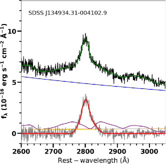
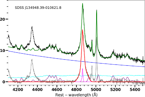
Figure 1.— Multi-component fitting results for the Mg II and H$\beta$ emission line regions. Left panel: example of Mg II fitting for the SDSS spectrum, SDSS J134934.31$-$004102.9. The rest-frame SDSS spectrum is in thick black. The total model (green) includes power-law continuum (blue), Fe II model (purple), and Balmer continuum model (orange). The continuum subtracted emission line is displayed in gray and the Mg II line model is presented in red. Right panel: example of H$\beta$ fitting for the SDSS spectrum, SDSS J134948.39$-$010621.8. The color schemes are the same as in the left panel, except that the stellar model is shown in cyan and narrow component of H$\beta$ is plotted in pink.

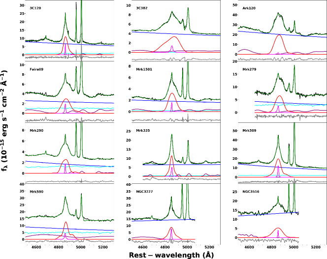
Figure 2.— Multi-component fitting results for the H$\beta$ emission line regions of 31 sources from Bahk et al. (2019). The total model (green) includes power-law continuum (blue), Fe II model (magenta), and Balmer continuum model (orange). The stellar model is shown in cyan and narrow component of H$\beta$ is plotted in pink. The continuum subtracted emission line is displayed in gray.

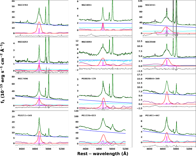
Figure 3.— Continue of Figure 2.

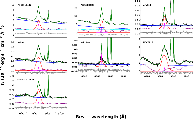
Figure 4.— Continue of Figure 3.

3.2. Line Profiles of Mg II and H$\beta$

In this section, we compare line width (FWHM) and line dispersion ($\sigma$) of the Mg II and H$\beta$ emission lines to investigate the characteristics of their line profiles (see Figure 7). As mentioned in Bahk et al. (2019), the Mg II emission line in the UV spectrum of NGC 4051 showed strong contamination by absorption features while this target has the smallest M_BH. Nonetheless, excluding or including this target in their analysis had no significant effect on the final results. Therefore, we included NGC 4051 in our analysis, but marked it with a different color for clarification in all the figures throughout the paper.

In the case of Mg II, the linear regression between FWHM and $\sigma$ shows a slope of 0.97 $\pm$ 0.03 with an intrinsic scatter $\sigma_{\mathrm{inst}}$ = 0.05 dex, indicating a linear relationship. The ratio of FWHM and $\sigma$ is in a range 1.23$-$3.91, with an average of 1.98 $\pm$ 0.34, which is smaller than the case of a Gaussian profile (i.e., 2.35). While the FWHM and $\sigma$ of Mg II show a linear relationship in general, we separated the sample into two groups for understanding the line profile of Mg II in more detail. We divided the sample at FWHM $=$ 3200 km s^-1, which is the mean value of the sample, and perform a linear regression. Separately, we found that the AGNs with narrower Mg II show a slope of 0.70 $\pm$ 0.04 ($\sigma_{\mathrm{inst}}$ = 0.03 dex), while the AGNs with broader Mg II have a slope of 0.91 $\pm$ 0.07 ($\sigma_{\mathrm{inst}}$ = 0.06 dex). This difference shows that there is significant change in the line profile between the narrow and broad Mg II lines. Narrower Mg II lines tend to have broader wings and a narrow core than broader Mg II lines.

In the case of H$\beta$, FWHM and $\sigma$ show a sub-linear relationship with a slope of 1.48 $\pm$ 0.03 ($\sigma_{\mathrm{inst}}$ = 0.06 dex). The ratio of FWHM and $\sigma$ is in a range of 1.03$-$3.53 with an average of 1.93 $\pm$ 0.40, which is similar to the case of Mg II, albeit with a larger scatter, 0.40 dex. We also separated the sample into two groups for understanding the line profile of H$\beta$ in more detail. We divided the sample at FWHM $=$ 4000 km s^-1, which is the mean value of the sample, and performed a linear regression. We found that the AGNs with narrower H$\beta$ show a slope of 1.16 $\pm$ 0.07 ($\sigma_{\mathrm{inst}}$ = 0.05 dex), while the AGNs with broader H$\beta$ have a slope of 1.25 $\pm$ 0.06 ($\sigma_{\mathrm{inst}}$ = 0.05 dex). In contrast with the Mg II profile, the two groups show consistent slopes. However, as a function of line width, the ratio of FWHM and $\sigma$ increases as line width increases. This result suggests that there is a systematic trend between the narrower and broader H$\beta$ lines.

In addition, we compared the difference of line profiles between H$\beta$ and Mg II as a function of line width. In the case of H$\beta$, we found that as the line width increases, FWHM-to-line dispersion ratio increases. We found a similar trend for Mg II, but with larger scatter. This result is consistent with those from our previous study with a limited luminosity range by Woo et al. (2018).

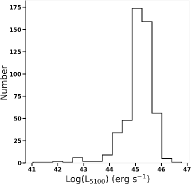
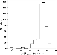
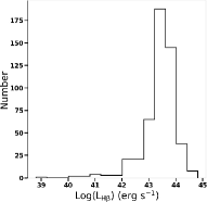
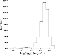
Figure 5.— Upper panels: Distributions of the $\mathrm{L_{5100}}$ (left panel) and $\mathrm{L_{3000}}$ (right panel). Bottom panels: Distributions of the $\mathrm{L_{H\beta}}$ (left panel) and $\mathrm{L_{MgII}}$ (right panel).

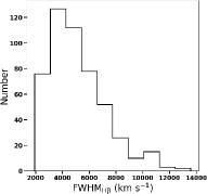
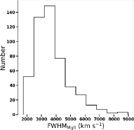
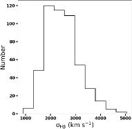
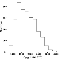
Figure 6.— Upper panels: Distributions of the line width $\rm FWHM_{H\beta}$ (left panel) and $\rm FWHM_{MgII}$ (right panel). Bottom panels: Distributions of the $\rm\sigma_{H\beta}$ (left panel) and $\rm\sigma_{MgII}$ (right panel).

4. Line Width and Luminosity Relations

We applied the cross correlation analysis for the line widths and luminosities. We used the FITEXY method (Park et al., 2012a; Woo et al., 2018) to find the best-fit results, including slope, intercept, and intrinsic scatter $\rm\sigma_{inst}$.

4.1. Line width comparison

In Figure 8, we compare the line widths between Mg II and H$\beta$ emission lines. In the case of $\sigma$, we found that Mg II $\sigma$ is narrower than that of H$\beta$ by $\sim$0.1 dex. The best-fit result is

$$\log\left(\frac{\sigma_{\rm Mg\sevenrm II}}{\rm 1000\ km\ s^{-1}}\right)=(-0.10\pm 0.01)$$ (3)

$$+\ (0.94\pm 0.03)\times\log\left(\frac{\sigma_{\rm H\beta}}{\rm 1000\ km\ s^{-1}}\right),$$

with an intrinsic scatter $\sigma_{\mathrm{inst}}$ = 0.06, indicating a linear relationship of $\sigma$ between Mg II and H$\beta$. The best-fit slope is consistent with our previous study of using 47 intermediate luminosity AGNs by Woo et al. (2018), who reported the best-fit slope 0.84 $\pm$ 0.07. This result is also consistent with that of Bahk et al. (2019), who obtained the slope of 0.89 $\pm$ 0.20 using low-luminosity reverberation-mapped AGNs.

In the case of FWHM, we found a shallower slope than that of line dispersion as:

$$\log\left(\frac{\rm FWHM_{\rm Mg\sevenrm II}}{\rm 1000\ km\ s^{-1}}\right)=(0.11\pm 0.01)$$ (4)

$$+\ (0.63\pm 0.02)\times\log\left(\frac{\rm FWHM_{\rm H\beta}}{\rm 1000\ km\ s^{-1}}\right),$$

with an intrinsic scatter $\sigma_{\mathrm{inst}}$ = 0.07. The best-fit slope is consistent with that of our previous work using moderate-luminosity AGNs (Woo et al., 2018), who reported a slope of 0.60 $\pm$ 0.07, while Wang et al. (2009) obtained a steeper slope of 0.81 $\pm$ 0.02. Note that Wang et al. (2009) subtracted the narrow component of Mg II in measuring of $\rm FWHM_{MgII}$. Thus, we expect the slope of Wang et al. (2009) is systematically steeper than that of ours since their $\rm FWHM_{MgII}$ could be overestimated.

To test the systematic difference between AGNs with broader and narrower lines, we divided the sample into two groups at FWHM $=$ 4000 km s^-1 (see Marziani et al., 2013). For the sources with narrower lines, the FWHMs of Mg II and H$\beta$ show comparable values to each other, while the best-fit slope is 0.59 $\pm$ 0.04 ($\sigma_{\mathrm{inst}}$ = 0.05). In contrast, AGNs with broader lines show a steeper slope of 0.70 $\pm$ 0.05 ($\sigma_{\mathrm{inst}}$ = 0.07) and Mg II line is typically narrower than H$\beta$. Our result is consistent with that of Marziani et al. (2013), who reported that $\rm FWHM_{H\beta}$ is broader than that of Mg II by $\sim$ 20$\%$. These results suggest systematic difference of the line profiles depending on the width of the line. In addition, we investigated the systematic effect on the slope due to the luminosity or Eddington ratio range. By dividing the sample into two subsamples using the median $\rm L_{3000}$ or the median Eddington ratio, we obtained the best fit for each subsample. However, we found no significant difference of the slope between these subsamples.

Since we found a sub-linear relationship between the FWHMs of H$\beta$ and Mg II, $\beta$ in Equation 2 cannot be the same for H$\beta$ and Mg II. In other words, if we use $\beta$ = 2 for H$\beta$ based on the virial assumption, we need to use $\beta$ ¿ 2 for Mg II, breaking the virial assumption. The nonlinear relationship between the FWHMs of H$\beta$ and Mg II raises large uncertainties in M_BH estimators. We also note that in the case of AGNs with a broad H$\beta$ line, the H$\beta$ line profile is complex, while the Mg II line profile shows no strong complexity (see Figure 4 in Woo et al., 2018). The asymmetry in the H$\beta$ line profile increases with increasing FWHM when FWHM is larger than 4000 km s^-1 (Wolf et al., 2019). Thus, the FWHM measurements and the M_BH estimates suffer from significantly large uncertainty when the line width is large. In contrast, we found no such trend in the case of line dispersion, which may suggest that M_BH estimators based on the line dispersion of H$\beta$ and Mg II provide better mass estimates.

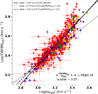
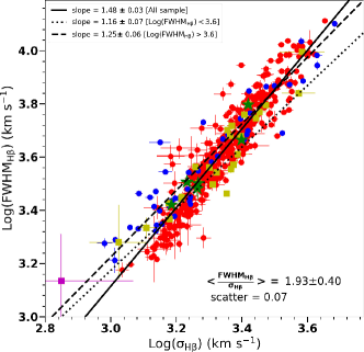
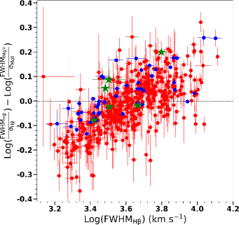
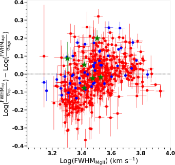
Figure 7.— Top left panel: comparison of the line width $\rm FWHM_{MgII}$ and line dispersion $\rm\sigma_{MgII}$. The best-fit slopes are presented for the total sample (solid line), AGNs with a broader Mg II, i.e., FWHM $>$ 3200 km s^-1(dashed line), and AGNs with a narrower Mg II, i.e., FWHM $<$ 3200 km s^-1(dotted line). The symbols represent the moderate-luminosity AGNs (blue), the SDSS sample (red) and the reverberation-mapped AGNs (yellow), the six HST targets (green), and NGC 4051 (pink). Top right panel: same as the top left panel, but for H$\beta$ emission line. Bottom panels: comparing the difference of line profile (FWHM and $\sigma$) between Mg II and H$\beta$ emission lines as a function of FWHM of H$\beta$ (left panel) and Mg II (right panel).

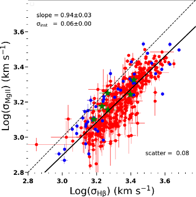
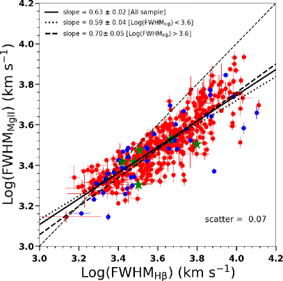
Figure 8.— Top panel: comparison of line dispersion $\rm\sigma_{MgII}$ and $\rm\sigma_{H\beta}$. Bottom panel: same as the top panel, but for the comparison of line width $\rm FWHM_{MgII}$ and $\rm FWHM_{H\beta}$. The best-fit slopes are presented for the total sample (solid line), AGNs with a broader H$\beta$, i.e., FWHM $>$ 4000 km s^-1(dashed line), and AGNs with a narrower Mg II, i.e., FWHM $<$ 4000 km s^-1(dotted line). The color schemes of sample are similar to those in Figure 7. The symbols are shown for the moderate-luminosity AGNs (blue), the SDSS sample (red), and the six HST targets (green).

4.2. Luminosity comparison

In Figure 9, we compare various continuum and emission line luminosities. First, we measured the best-fit slope between $\mathrm{L_{H\beta}}$ and $\mathrm{L_{5100}}$ as,

$$\log\left(\frac{\rm L_{\rm H\beta}}{\rm 10^{42}\ erg\ s^{-1}}\right)=(0.31\pm 0.02)$$ (5)

$$+\ (0.98\pm 0.02)\times\log\left(\frac{\rm L_{\rm 5100}}{\rm 10^{44}\ erg\ s^{-1}}\right),$$

with $\sigma_{\mathrm{inst}}$ = 0.19 $\pm$ 0.01. This slope indicates a linear relationship between $\mathrm{L_{H\beta}}$ and $\mathrm{L_{5100}}$, and which is consistent with our previous work by Woo et al. (2018) while the slope is shallower than 1.13 $\pm$ 0.01 reported by Greene & Ho (2005). Using only high luminosity sample, $\rm\log\lambda L_{5100}\$¿$\ 45.4$ erg s^-1, in contrast, Shen & Liu (2012) presented a much steeper slope of 1.25 $\pm$ 0.07. The large dynamic range of our sample may overcome any systematic trend implemented in a limited luminosity range.

Second, we compared $\mathrm{L_{3000}}$ with $\mathrm{L_{5100}}$, and obtained the best-fit result as,

$$\log\left(\frac{\rm L_{3000}}{\rm 10^{44}\ erg\ s^{-1}}\right)=(0.29\pm 0.01)$$ (6)

$$+\ (0.98\pm 0.02)\times\log\left(\frac{\rm L_{\rm 5100}}{\rm 10^{44}\ erg\ s^{-1}}\right),$$

with $\sigma_{\mathrm{inst}}$ = 0.13 $\pm$ 0.01, being consistent with the result of our previous work (Woo et al., 2018). Our result is also consistent with that of Shen & Liu (2012), who presented a slope of 0.98 $\pm$ 0.01.

Third, we compared the Mg II line luminosity with H$\beta$ and continuum luminosities. The best-fit slopes show somewhat sub-linear relationships between those luminosities as

$$\log\left(\frac{\rm L_{\rm Mg\sevenrm II}}{\rm 10^{42}\ erg\ s^{-1}}\right)=(0.43\pm 0.02)$$ (7)

$$+\ (0.82\pm 0.02)\times\log\left(\frac{\rm L_{\rm 5100}}{\rm 10^{44}\ erg\ s^{-1}}\right),$$

with $\sigma_{\mathrm{inst}}$ = 0.23 $\pm$ 0.01,

$$\log\left(\frac{\rm L_{\rm Mg\sevenrm II}}{\rm 10^{42}\ erg\ s^{-1}}\right)=(0.14\pm 0.03)$$ (8)

$$+\ (0.87\pm 0.02)\times\log\left(\frac{\rm L_{\rm 3000}}{\rm 10^{44}\ erg\ s^{-1}}\right),$$

with $\sigma_{\mathrm{inst}}$ = 0.18 $\pm$ 0.01,

$$\log\left(\frac{\rm L_{\rm Mg\sevenrm II}}{\rm 10^{42}\ erg\ s^{-1}}\right)=(0.14\pm 0.02)$$ (9)

$$+\ (0.87\pm 0.02)\times\log\left(\frac{\rm L_{\rm H\beta}}{\rm 10^{42}\ erg\ s^{-1}}\right),$$

with $\sigma_{\mathrm{inst}}$ = 0.17 $\pm$ 0.01, respectively. These results are consistent with our previous study with moderate-luminosity AGNs (Woo et al., 2018). The relationship between $\rm L_{Mg\sevenrm II}$ and $\mathrm{L_{5100}}$ is also consistent with that of Shen & Liu (2012), who reported a slope of 0.86 $\pm$ 0.07. In the case of $\rm L_{Mg\sevenrm II}$ with $\mathrm{L_{3000}}$, we obtained a shallower slope than that of Shen et al. (2011), who showed a slope of 0.98. We expect that the discrepancy is from the difference of luminosity range in the sample. Shen et al. (2011) used the high-luminosity SDSS sample, while our sample has a much broader luminosity range. This indicates that there is significant change in the line profile of Mg II. This significant change is also shown in the comparison between FWHM and line dispersion $\sigma$ of Mg II in Figure 7.

The comparison between line and continuum luminosity is consistent with that of Dong et al. (2009) who reported a sub-linear relationship between $\rm L_{Mg\sevenrm II}$ and $\mathrm{L_{3000}}$ with a slope of 0.91$\pm$ 0.01. Dong et al. (2009) explained that the sub-linear relationship indicates the Baldwin effect (Baldwin, 1977) in the UV range since for higher luminosity AGNs, the continuum luminosity near the Big Blue Bump will be higher because of the increase of the thermal component in the UV continuum (e.g., Malkan & Sargent, 1982; Zheng & Malkan, 1993).

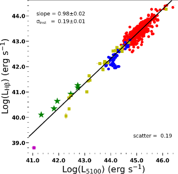
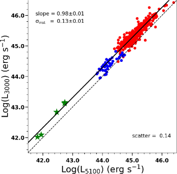
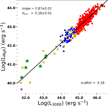
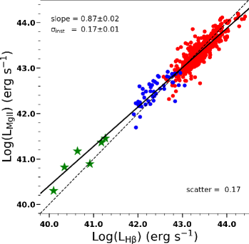
Figure 9.— Comparison of continuum and emission line luminosities. Top panels: comparing $\rm L_{5100}$ with $\rm L_{H\beta}$ (left) and $\rm L_{3000}$ (right). Bottom panels: Same as those top panels, but for the comparison of for $\rm L_{3000}$ vs. $\rm L_{MgII}$ (left) and $\rm L_{H\beta}$ vs. $\rm L_{MgII}$ (right). The symbols are shown for the moderate-luminosity AGNs (blue), the SDSS sample (red), the 25 RM sources (yellow), the six HST targets (green), and NGC 4051 (pink). The best-fit slope is shown in thick black solid line. The dash-lines represent one to one relation.

Table 1 Optical spectral properties of 31 sample

Target	z	Ref	Date-observation	Gap	S/N	$\rm FWHM_{H\beta}$	$\rm\sigma_{H\beta}$	$\rm\log\lambda L_{5100}$	$\rm\log L_{H\beta}$
(1)	(2)	(3)	(4)	(5)	(6)	(7)	(8)	(9)	10
3C120	0.033	M03	24 Sep 1995	11	39	2673 $\pm$ 45	1505 $\pm$ 21	43.886 $\pm$ 0.001	42.157 $\pm$ 0.004
3C382	0.058	B09	10 Aug 2007	4	30	9906 $\pm$ 425	3831 $\pm$ 612	44.182 $\pm$ 0.005	42.635 $\pm$ 0.026
Ark120	0.033	M03	03 Apr 1990	5	45	5754 $\pm$ 66	2554 $\pm$ 43	44.367 $\pm$ 0.002	42.684 $\pm$ 0.005
Fairall9	0.047	M03	20 Dec 1993	0.1	40	5575 $\pm$ 120	2769 $\pm$ 41	43.768 $\pm$ 0.044	42.203 $\pm$ 0.006
Mrk1501	0.089	M03	08 Oct 1994	2	43	5037 $\pm$ 66	2266 $\pm$ 47	44.238 $\pm$ 0.016	42.757 $\pm$ 0.004
Mrk279	0.031	M03	26 Mar 1989	11	25	5236 $\pm$ 208	2343 $\pm$ 85	43.581 $\pm$ 0.133	42.121 $\pm$ 0.021
Mrk290	0.030	M03	16 Feb 1990	5	45	4789 $\pm$ 65	2314 $\pm$ 68	43.168 $\pm$ 0.024	41.640 $\pm$ 0.007
Mrk335	0.026	M03	13 Oct 1996	11	39	2158 $\pm$ 199	1284 $\pm$ 83	43.706 $\pm$ 0.035	41.877 $\pm$ 0.015
Mrk509	0.034	M03	12 Oct 1996	4	51	3733 $\pm$ 42	2364 $\pm$ 28	44.097 $\pm$ 0.011	42.613 $\pm$ 0.002
Mrk590	0.026	M03	13 Oct 1996	5	48	2911 $\pm$ 74	2256 $\pm$ 45	43.756 $\pm$ 0.013	42.136 $\pm$ 0.005
NGC3227	0.004	Ho95	29 Mar 1986	14	20	3647 $\pm$ 267	1995 $\pm$ 105	42.396 $\pm$ 0.003	40.332 $\pm$ 0.013
NGC3516	0.009	Ho95	29 Mar 1986	10	20	6253 $\pm$ 221	2969 $\pm$ 172	43.083 $\pm$ 0.003	41.006 $\pm$ 0.015
NGC3783	0.010	M03	23 May 1993	1	42	3654 $\pm$ 70	1811 $\pm$ 58	43.209 $\pm$ 0.010	41.464 $\pm$ 0.006
NGC4051	0.002	M06	$\cdots$	$\cdots$	20	1366 $\pm$ 551	707 $\pm$ 357	41.050 $\pm$ 0.096	38.802 $\pm$ 0.074
NGC4151	0.003	M03	01 Jul 1995	5	28	6922 $\pm$ 218	3738 $\pm$ 442	42.467 $\pm$ 0.002	40.858 $\pm$ 0.082
NGC4253	0.013	M03	25 June 2001	1	19	1908 $\pm$ 613	1056 $\pm$ 217	42.279 $\pm$ 0.032	40.057 $\pm$ 0.120
NGC4593	0.009	M03	04 Apr 1990	3	26	4785 $\pm$ 135	2489 $\pm$ 121	42.391 $\pm$ 0.071	40.766 $\pm$ 0.016
NGC5548	0.017	M03	21 May 1993	1	35	5884 $\pm$ 262	2839 $\pm$ 139	43.133 $\pm$ 0.078	41.432 $\pm$ 0.014
NGC7496	0.016	M03	12 Oct 1996	0.3	37	3595 $\pm$ 127	2324 $\pm$ 63	43.700 $\pm$ 0.009	41.900 $\pm$ 0.006
PG0026+129	0.142	M03	11 Oct 1990	4	47	3141 $\pm$ 192	2046 $\pm$ 86	44.439 $\pm$ 0.039	42.798 $\pm$ 0.007
PG0844+349	0.064	M03	22 Feb 1991	1	44	2783 $\pm$ 48	1638 $\pm$ 29	44.438 $\pm$ 0.001	42.603 $\pm$ 0.005
PG1211+143	0.081	M03	01 May 1995	4	42	2336 $\pm$ 74	1512 $\pm$ 41	44.701 $\pm$ 0.002	42.950 $\pm$ 0.006
PG1226+023	0.158	M03	04 Apr 1990	9	30	4091 $\pm$ 344	2435 $\pm$ 199	46.135 $\pm$ 0.080	44.268 $\pm$ 0.020
PG1411+442	0.090	M03	23 Jun 2001	0.3	44	3491 $\pm$ 372	2103 $\pm$ 125	44.443 $\pm$ 0.017	42.728 $\pm$ 0.011
PG2130+099	0.063	M03	18 Sep 1990	6	40	2824 $\pm$ 86	1645 $\pm$ 42	44.093 $\pm$ 0.042	42.616 $\pm$ 0.008
Arp151	0.021	B19	29 Apr 2013	0	17	3039 $\pm$ 199	1837 $\pm$ 101	41.943 $\pm$ 0.010	40.637 $\pm$ 0.011
Mrk50	0.023	B19	12 Dec 2012	0	19	4633 $\pm$ 122	2502 $\pm$ 107	42.731 $\pm$ 0.005	41.174 $\pm$ 0.009
Mrk1310	0.020	B19	07 Jan 2013	0	14	3179 $\pm$ 487	1847 $\pm$ 171	41.818 $\pm$ 0.013	40.345 $\pm$ 0.025
NGC6814	0.005	B19	07 Jan 2013	0	20	6274 $\pm$ 95	2622 $\pm$ 52	41.331 $\pm$ 0.007	40.100 $\pm$ 0.005
SBS1116+583A	0.028	B19	12 Jul 2013	0	13	3215 $\pm$ 103	1706 $\pm$ 71	42.466 $\pm$ 0.006	40.917 $\pm$ 0.008
Zw229-015	0.028	B19	23 Jul 2013	0	18	2638 $\pm$ 49	1529 $\pm$ 37	42.734 $\pm$ 0.005	41.262 $\pm$ 0.006

5. Calibrating M_BH estimators

In this section, we calibrate M_BH estimators for each pair of velocity and luminosity from Mg II, H$\beta$, $\rm L_{3000}$ and $\rm L_{5100}$, using the best fits from Section 4. We determined the parameters in Equation 2 by comparing with the fiducial M_BH. As a reference, we used two fiducial masses. The first fiducial mass is determined from $\rm\sigma_{H\beta}$ and $\rm L_{5100}$, and the second fiducial mass is obtained from $\rm FWHM_{H\beta}$ and $\rm L_{5100}$. As in our previous study in Woo et al. (2018), we adopted the virial theorem and H$\beta$ size-luminosity relation ($\beta=2.0$ and $\gamma=0.533$) for calculating fiducial masses. For the virial factor, we used the best-fit value f = 4.47 ($\alpha$ = 7.47) and f = 1.12 ($\alpha$ = 6.87) from Woo et al. (2015), respectively, for the fiducial masses based on $\rm\sigma_{H\beta}$ and $\rm FWHM_{H\beta}$.

5.1. H$\beta$-based mass estimators

In Figure 10, we present the M_BH estimator based on the H$\beta$ emission line. Firstly, in the case of the fiducial mass based on the H$\beta$ line dispersion $\rm\sigma_{H\beta}$ and $\rm L_{5100}$, we fixed $\beta=2.0$ for $\rm\sigma_{H\beta}$, and for $\rm FWHM_{H\beta}$, we fixed $\beta=2.0/1.48=1.35$ (based on the obtained slopes of $\rm FWHM_{H\beta}$ and $\rm\sigma_{H\beta}$ in Figure 7). Secondly, when the fiducial mass is based on $\rm FWHM_{H\beta}$ and $\rm L_{5100}$, we fixed $\beta=2.0$ for $\rm FWHM_{H\beta}$, and for $\rm\sigma_{H\beta}$, we fixed $\beta=2.0/(1.0/1.48)=2.96$. For both fiducial masses, we used $\gamma$ = 0.533/0.98 = 0.55 when adopting luminosity from $\rm L_{H\beta}$ (Figure 9). Using those $\beta$ and $\gamma$ values, we determined $\alpha$ based on the $\chi^{2}$ minimization with the FITEXY method in Park et al. (2012b). The root-mean-square (rms) scatters of both M_BH estimators are 0.10$-$0.13 dex and 0.10$-$0.19 dex for the fiducial masses from $\rm\sigma_{H\beta}$ and $\rm FWHM_{H\beta}$, respectively. When luminosity is adopted from the H$\beta$ emission line, the rms scatter becomes larger compared to that of using continuum 5100Å luminosity. Similarly, the choice of velocity by using $\rm FWHM_{H\beta}$ has larger rms scatter than when $\rm\sigma_{H\beta}$ is used as velocity. By enlarging the sample using SDSS, our estimators have slightly smaller rms scatter ($\sim$0.05 dex) compared to that of our previous study in Woo et al. (2018).

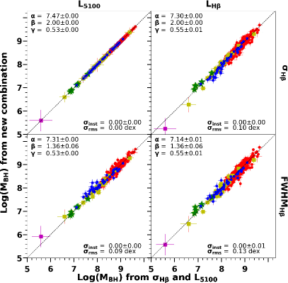
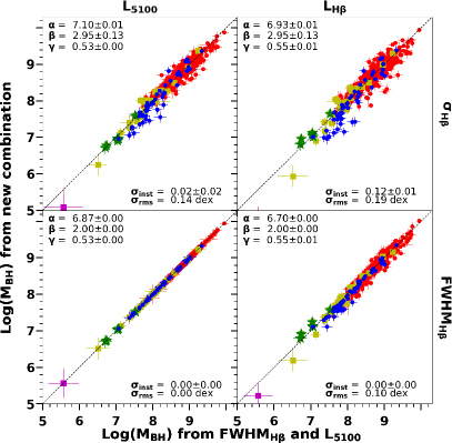
Figure 10.— Newly derived M_BH with estimator from H$\beta$ emission line. Left panel: cross-calibration fitting between newly derived M_BH and the fiducial mass with estimator based on $\sigma_{\rm H\beta}$ and $\rm L_{5100}$. Newly derived M_BH is from $\rm\alpha+\beta\log V_{1000}+\gamma\log L$. $\rm V_{1000}$ is velocity estimator in units of $\rm 1000~{}km~{}s^{-1}$, L is luminosity estimator in units of $\rm 10^{44}~{}erg~{}s^{-1}$ for continuum or $\rm 10^{42}~{}erg~{}s^{-1}$ for emission line. $\alpha$ is estimated by $\chi^{2}$ minimization fitting. $\beta$ and $\gamma$ in each panel depend on different estimators, shown in the top and upper right part of each figure. Right panel: same as the left panel, but for the fiducial mass with estimator based on $\rm FWHM_{\rm H\beta}$ and $\rm L_{5100}$. The symbols are shown for the moderate-luminosity AGNs (blue), the SDSS sample (red), the 25 RM sources (yellow), the six HST targets (green), and NGC 4051 (pink). The dash-lines represent one to one relation.

5.2. Mg II-based mass estimators

We calibrated the M_BH estimators based on the Mg II emission line by determining $\alpha$, $\beta$, and $\gamma$ in Equation 2. As we performed in our previous study (Woo et al., 2018), we used five schemes in the fitting process:
     $\bullet$ Scheme 1: $\beta$ and $\gamma$ are adopted from scaling relations in Section 4.
      $\bullet$ Scheme 2: $\beta=2.0$ and $\gamma=0.5$.
      $\bullet$ Scheme 3: $\beta=2.0$ and $\gamma$ is a free parameter.
      $\bullet$ Scheme 4: $\gamma=0.5$ and $\beta$ is a free parameter.
      $\bullet$ Scheme 5: both $\beta$ and $\gamma$ are free parameters.

We present all calibrated parameters for these five Schemes in Tables 2 and 3 based on the fiducial masses from $\rm\sigma_{H\beta}$ and $\rm FWHM_{H\beta}$, respectively. In Figure 11, we show 3 cases (Schemes 1, 2, and 5). In total, we have 25 AGNs, for which UV and optical spectra were not observed simultaneously. By excluding these 25 AGNs, we performed the calibration of M_BH estimators. However, we found consistent results with/without these 25 AGNs. Therefore, we presented the calibration results for the total sample. Note that we presented the results based on the FITEXY method to be consistent with our previous studies. However, we also used the Bayesian method using PYMC (Python Markov chain Monte Carlo), and obtained consistent results.

In the case of Scheme 1, $\beta$ and $\gamma$ were fixed as determined from the scaling relations in Sections 4.1 and 4.2. With respect to the fiducial mass based on the H$\beta$ line dispersion, we obtained $\beta=2/0.94=2.13$ for $\rm\sigma_{MgII}$ because of log $\sigma_{\rm MgII}$ $\propto$ 0.94 log $\rm\sigma_{H\beta}$ in Equation 3. For $\rm FWHM_{MgII}$, we adopted $\beta=2.0/0.93=2.14$ since log FWHM_MgII $\propto$ 0.93 log $\rm\sigma_{H\beta}$. When we used the fiducial mass based on $\rm FWHM_{H\beta}$, we fixed $\beta=2.0/0.63=3.17$ for $\rm FWHM_{MgII}$ because of Equation 4, and $\beta=2.0/0.625=3.20$ for $\rm\sigma_{MgII}$ because of log $\sigma_{\rm MgII}$ $\propto$ 0.625 log $\rm FWHM_{H\beta}$. For $\gamma$, we also used the scaling relation. For example, we obtained $\gamma$ = 0.533/0.98 = 0.54 for $\rm L_{3000}$, and $\gamma$ = 0.533/0.82 = 0.65 for $\rm L_{MgII}$, using the best-fit slopes in Equations 6 and 7, respectively.

The results of Scheme 1 show that the M_BH estimators based on $\sigma_{\rm MgII}$ have a rms scatter of 0.19$-$0.25 dex, which is smaller than the case of M_BH estimators based on $\rm FWHM_{MgII}$, 0.25$-$0.31 dex (see Figure 11). In general, the rms scatter becomes larger when we adopted $\rm L_{MgII}$ and $\rm FWHM_{MgII}$, indicating that the pair of continuum luminosity from 3000Å and $\rm\sigma_{MgII}$ is the best choice for the UV M_BH estimator. By enlarging the sample size and the dynamic range of AGN luminosity, the calibration is improved as the rms scatters become smaller than that of our previous study (Woo et al., 2018) by $\sim$ 0.05$-$0.1 dex.

In the cases of Schemes 2 and 3, we fixed $\beta=2.0$ and set $\gamma$ as a free parameter (Scheme 3) or fixed both $\beta=2.0$ and $\gamma=0.5$ (Scheme 2), following the virial theorem and expected size-luminosity relation. With respect to the fiducial mass based on the H$\beta$ line dispersion, we obtained a smaller rms scatter, 0.18$-$0.23 dex than that of the Scheme 1. Compared to the previous study by Woo et al. (2018), the rms scatter is reduced by 0.03$-$0.06 dex. When we adopted the fiducial mass based on $\rm FWHM_{H\beta}$, the rms scatter is 0.22$-$0.24 dex, which is also smaller than that of Woo et al. (2018) by 0.01$-$0.08 dex.

Turning to the cases of Schemes 4 and 5, we fixed $\gamma=0.5$ and set $\beta$ as a free parameter (Scheme 4) or set both of them as free parameters (Scheme 5). The obtained rms scatters for Schemes 4 and 5 are slightly smaller compared to those of Schemes 2 and 3 by $\sim$ 0.02$-$0.04 dex.

In the case of the fiducial mass by $\rm FWHM_{\rm H\beta}$ and $\rm L_{5100}$ (see Table 3), our calibration is improved with smaller intrinsic scatter (0.14$-$0.25 dex) and rms scatter (0.21$-$0.30 dex) than those in our previous studies (Woo et al., 2018). Nevertheless, the calibration based on the fiducial mass from $\rm FWHM_{\rm H\beta}$ and $\rm L_{5100}$ is less reliable with a larger scatter, compared to the M_BH estimators based on the fiducial mass from $\sigma_{\rm H\beta}$ and $\rm L_{5100}$.

Based on our results, we found that the best M_BH estimator based on Mg II is achieved when using $\sigma_{\rm MgII}$ and $\rm L_{3000}$, with smallest intrinsic and rms scatters ($\rm\sigma_{inst}$ = 0.09-0.12 dex and $\rm\sigma_{rms}$ = 0.17-0.20 dex). Among the five Schemes, we found that Schemes 2, 3, 4 and 5 give small $\rm\sigma_{inst}$ and $\rm\sigma_{rms}$, 0.09 and 0.17 dex, respectively. However, in those Schemes 4 and 5, $\beta\sim 1.5$ breaks the virial relation ($\beta=2.0$). The two other cases (Schemes 2 and 3) show similar $\rm\sigma_{inst}$ and $\rm\sigma_{rms}$, 0.11 and 0.19 dex, respectively. However, we recommend Scheme 2 as the best Mg II M_BH estimator since it follows the virial relation and the expected size-luminosity relation ($\beta=2.0$ and $\gamma=0.5$).

In short, by enlarging the sample over a large luminosity range, we improve the calibration of Mg II based mass estimators. For the best pair of L₃₀₀₀ and line dispersion of Mg II ($\sigma_{\rm MgII}$), we found an intrinsic scatter of $\sim$0.1 dex and a rms scatter of $\sim$0.2 dex, indicating that the M_BH estimated based on the Mg II line and UV continuum luminosity is only slightly less reliable compared to the M_BH based on the H$\beta$ line and L₅₁₀₀.

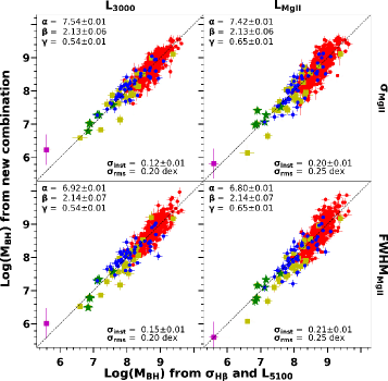
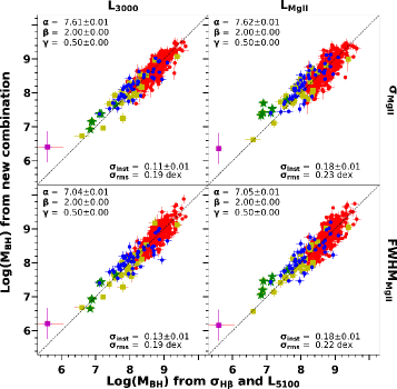
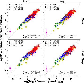
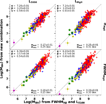
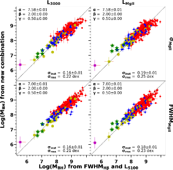
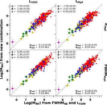
Figure 11.— Same as Figure 10, but for M_BH estimator from Mg II. Top panels: cross-calibration fitting between newly derived M_BH and fiducial mass with estimator based on $\sigma_{\rm H\beta}$ and $\rm L_{5100}$. $\beta$ and $\gamma$ is obtained from scaling relations of line width and luminosity in Sections 4.1 and 4.2 (top left panel). Top middle panel: $\beta$ is 2.0, based on the virial assumption and $\gamma$ is 0.5, from expected size-luminosity relation. Top right panel: $\beta$ and $\gamma$ is obtained from the best-fit results based on Scheme 5 in Section 5.2. Bottom panels: same as the top panels, but for the fiducial mass with estimator based on $\rm FWHM_{\rm H\beta}$ and $\rm L_{5100}$. The symbols are shown for the moderate-luminosity AGNs (blue), the SDSS sample (red), the 25 RM sources (yellow), the six HST targets (green), and NGC 4051 (pink). The dash-lines represent one to one relation.

6. Discussion

6.1. Uncertainties of the Mg II-based mass

In this section we discuss the systematic uncertainties of the calibrated Mg II M_BH estimators. For simplicity, we present the results from Scheme 2 for this comparison. Note that we also investigated the systematic uncertainties using the other 4 Schemes and obtained the consistent results. Figure 12 shows the systematic difference between UV and optical M_BH estimators as a function of AGN properties. We found no significant correlation of the M_BH difference with Eddington ratio, $\rm FWHM_{H\beta}$, F_OIII/F_FeII, and F_OIII/F_Hβ,narrow. However, we found that the difference between Mg II and H$\beta$-based masses anti-correlates with the systematic difference of the line profiles ($\Delta\rm P$) between Mg II and H$\beta$, which is parameterized by the ratio between FWHM and line dispersion. By performing a regression analysis, we obtained the best-fit result:

$$\Delta\rm P=-0.83\times\log\left(\frac{\rm FWHM_{MgII}/\sigma_{MgII}}{\rm FWHM_{H\beta}/\sigma_{H\beta}}\right)-0.01.$$ (10)

We also found a positive correlation between the mass difference and the UV-to-optical continuum luminosity ratio as similarly reported by Woo et al. (2018). We obtained the best-fit slope of 0.73 $\pm$ 0.05 and the intercept of 0.21 $\pm$ 0.02 when comparing the systematic differences of the UV and optical M_BH estimates with the UV-to-optical luminosity ratios. Similar to our previous work, in order to minimize the systematic effect to the different slope of the UV-to-optical spectral slope, we propose to add this correction term to the Equation 2:

$$\Delta\rm C=-0.73\times\log(\rm L_{3000}/L_{5100})+0.21,$$ (11)

As similarly suggested by Woo et al. (2018) based on the modeling of the local UV/optical AGN continuum using a power law function, we derived the correction factor as a function of the power law coefficient of the AGN continuum $\alpha_{\lambda}$:

$$\Delta\rm C=0.17(1+\alpha_{\lambda})+0.20.$$ (12)

where, the mean $\alpha_{\lambda}$ of our sample is -2.69 $\pm$ 0.87 (i.e., $\alpha_{\nu}$ = 0.69 $\pm$ 0.87). We measured this $\alpha_{\lambda}$ in the wavelength range of 2800-5200 Å. Note that this correction for M_BH is relative small, $\sim$0.1 dex. In practice the observed spectrum is likely to be limited in the rest-frame UV for high-z AGNs, and if so, the spectral slope cannot be measured from the 2800-5200 Å range. Thus, we present the effect of the different spectral slope as a bias in the M_BH estimation.

The difference in the line profiles between Mg II and H$\beta$ has a significant effect on the M_BH estimation. The nonlinear relationship between $\rm FWHM_{MgII}$ and $\rm FWHM_{H\beta}$ will have a significant effect in the UV and optical M_BH estimators. Particularly, as in Figure 8, the different slopes between the narrow and broad $\rm FWHM_{MgII}$ sample shows significant changes in the line profiles of H$\beta$ and Mg II  hence will raise systematic uncertainty between the Mg II and H$\beta$ M_BH estimators. We found that the discrepancy between Mg II and H$\beta$-based masses shows a negative correlation with the line profile of Mg II (Figure 13). Since the line profile of Mg II has significant effect on the difference of the Mg II and H$\beta$-based masses, we also suggest a correction factor, $\Delta\rm M$ based on the best-fit result as follow:

$$\Delta\rm M=-1.14\times\log\left(\frac{\rm FWHM_{MgII}}{\sigma_{MgII}}\right)+0.33.$$ (13)

To demonstrate the effect of the color-correction term and the correction term of Mg II line profile, we compared the Mg II and H$\beta$-based M_BH with the corrections of $\rm\Delta C$, $\rm\Delta M$ and the combination of them in Figure 14. We found that the systematic uncertainty, i.e., the rms scatter between the UV and optical M_BH can be reduced from 0.19 dex to 0.15 dex. In practice, when only the rest-frame UV spectrum is available for estimating M_BH, the correction term $\Delta\rm M$ would be useful since $\Delta\rm C$ or $\Delta\rm P$ cannot be obtained without the rest-frame optical spectrum.

We have presented that the change of the UV-to-optical continuum luminosity and the difference of the line profile between H$\beta$ and Mg II cause a large systematic difference between the Mg II and H$\beta$ M_BH estimators. In addition, we list here sources of systematic uncertainties, which could bias the Mg II M_BH estimator. First, as we mentioned in Section 1, there is no available size-luminosity relation based on Mg II emission line. In this study, we calibrated the Mg II M_BH estimator based on the fiducial mass as the single-epoch H$\beta$ based mass based on the size-luminosity relation which has an uncertainty, $\sim$0.19 dex Bentz et al. (2013). Second, the uncertainty of the virial factor f is $\sim$0.12-0.40 dex (e.g., Woo et al., 2015; Pancoast et al., 2014). Third, the variability between the line width and luminosity could introduce a bias with scatter of $\sim$0.1 dex (Park et al., 2012a). Therefore, we keep in mind that we estimated the Mg II M_BH estimator that is calibrated based on the fiducial mass which has also various uncertainties of itself, $\sim$0.40-0.70 dex.

We note that there are also significant uncertainties of the M_BH estimator based on the analysis of Mg II line. First, luminosity and velocity in AGNs show variability. This variability could bias the Mg II M_BH estimator based on the H$\beta$ based mass if the rest-frame spectra of the UV and optical are not observed at the same time. Second, there are reports that the line width FWHMs of H$\beta$ and Mg II are not comparable, and $\rm FWHM_{H\beta}$ is larger than that of Mg II by $\sim 20\%$ for the broad H$\beta$ line AGNs (e.g., Marziani et al., 2013, also see Figure 8 in Section 4). We adopted the virial relation, and apply the same $\beta=2.0$ for the H$\beta$ and Mg II based masses, respectively. This could bias the Mg II M_BH estimator since $\rm FWHM_{H\beta}$ is larger than that of Mg II, and $\beta$ value needs to be higher than 2.0. Third, the measurements of the Mg II line could introduce a bias in the Mg II M_BH estimator. For example, a careful analysis of fitting and subtracting for Balmer continuum in the UV spectra may be required for an accurate determination of $\rm L_{3000}$ (Kovačević-Dojčinović et al., 2017). Fourth, in our analysis, we did not subtract the narrow component of Mg II since there is no clear narrow Mg II component in our spectra. We note that subtracting the narrow component of Mg II should be performed with caution since it is difficult to determine how much the narrow component contributes to the line profile.

6.2. Comparison with previous Mg II-based M_BH estimators

There have been various M_BH estimators based on the Mg II emission line in the literature (e.g., McGill et al., 2008; Wang et al., 2009; Shen et al., 2011; Shen & Liu, 2012; Tilton & Shull, 2013; Woo et al., 2018; Bahk et al., 2019). As detailed by Woo et al. (2018), the difference among these M_BH estimators is originated by various factors, i.e., Fe II templates, the narrow component of Mg II, and the virial factor f. For example, we adopted the Fe II template from Tsuzuki et al. (2006) while other studies such as Shen et al. (2011) and Shen & Liu (2012) used the Fe II template from Vestergaard & Wilkes (2001) and Salviander et al. (2007), respectively. The line dispersion of Mg II becomes smaller if the Fe II template from Tsuzuki et al. (2006) is adopted in the fitting process (see Figure 2 in Woo et al., 2018). Also, Shin et al. (2019) pointed out that the flux ratio of Fe II/Mg II could be different up to $\sim$0.2 dex between the Fe II modeled by Tsuzuki et al. (2006) and Vestergaard & Wilkes (2001). Regarding the measurement of FWHM, the subtraction of the potential narrow component in Mg II significantly changes the result as we mentioned in Section 3.1. For example, as Wang et al. (2009) subtracted the narrow component in their Mg II model, their FWHM measurements could be systematically different from our measurement. In addition, using a different scaling factor f also causes discrepancies between M_BH mass estimators. In this section, we determined M_BH using various mass estimators and compared them to previous studies to investigate systematic differences, using the measurements of the FWHM and line dispersion of Mg II line as well as continuum luminosity at 3000Å and Mg II line luminosity. For this comparison we chose the results based on Scheme 2 as the best Mg II M_BH estimator from our calibration.

First, we note that our new calibration is very close to that presented by Woo et al. (2018), who used only intermediate luminosity AGNs. In the calibration with the fiducial mass from the pair of $\sigma_{\rm H\beta}$ and $\rm L_{5100}$, both intrinsic scatter (0.09$-$0.21 dex) and rms scatter (0.17$-$0.25 dex) become smaller than those reported by Woo et al. (2018), i.e., $\rm\sigma_{inst}$ = 0.13$-$0.23 dex and $\rm\sigma_{rms}$ = 0.18$-$0.36 dex. When we used the fiducial mass based on $\rm FWHM_{\rm H\beta}$ and $\rm L_{5100}$, we also obtained consistent mass estimators compared to those of Woo et al. (2018), with slightly improved scatters by $\rm\sigma_{inst}$ = 0.14$-$0.26 dex and $\rm\sigma_{rms}$ = 0.21$-$0.31 dex.

We compared our results with that of Bahk et al. (2019), the 31 H$\beta$ RM AGNs are applied by the same method as we did in our Scheme 2. However, there is systematic difference between our estimator and that of Bahk et al. (2019) with an offset of $\sim$0.27 dex. In Bahk et al. (2019), the authors discussed that the large systematic difference between the two estimators is from the difference of $\sigma_{\rm H\beta}$/$\sigma_{\rm MgII}$ and $\rm L_{5100}$/$\rm L_{3000}$. This result indicates that there is a systematic uncertainty in the Mg II-based M_BH estimator which is raised from the different line profiles between the Mg II and H$\beta$ emission lines. The relation between the UV and optical mass estimator ratio and the systematic difference of the line profiles between Mg II and H$\beta$, shown in Figure 12, support this argument.

Second, we compared our mass estimator with the previously reported estimators by Wang et al. (2009), Shen et al. (2011), Shen & Liu (2012) and Tilton & Shull (2013) in Figure 15. In this comparison, we adjusted the $\alpha$ values of other works by -0.09 dex since they adopted $\log$f = 0.74 from (Onken et al., 2004). Since these studies only provided the measurements of FWHM of Mg II, we compared M_BH based on $\rm FWHM_{MgII}$ and L₃₀₀₀.

We found our M_BH is systematically larger by $\sim$0.25 dex than the M_BH calculated with the recipes from Wang et al. (2009), Shen et al. (2011) and Shen & Liu (2012). For the case of using $\rm FWHM_{MgII}$ and $\rm L_{MgII}$, our estimator has a large offset of 0.33 dex compared to that of Tilton & Shull (2013).

The M_BH based on our best estimator is higher than that based on the recipe of Wang et al. (2009) by 0.25 dex. As we mentioned, Wang et al. (2009) subtracted the narrow component in the modeling of the Mg II line profile. Thus, $\rm FWHM_{MgII}$ is systematically higher in their analysis, leading to a smaller $\alpha$ for comparison with given fiducial M_BH. Compared to the mass estimators presented by Shen et al. (2011) and Shen & Liu (2012), our mass estimator provides higher M_BH by 0.22$-$0.25 dex. Similar to Wang et al. (2009), Shen et al. (2011) and Shen & Liu (2012) subtracted the narrow component of Mg II, which lead to a smaller $\alpha$ in Equation 2 compared to our M_BH estimator. In contrast, M_BH is more consistent between our estimator and the estimators of Shen et al. (2011) and Shen & Liu (2012). This is due to the limited luminosity range of their calibrations. Shen et al. (2011) used a high luminosity sample from SDSS ($\rm L_{5100}>10^{44}\ ergs^{-1}$) at z = 0.4$-$0.8, while Shen & Liu (2012) utilized higher luminosity sample ($\rm L_{5100}>10^{45.4}\ ergs^{-1}$) at z = 1.5$-$2.2. Therefore, these M_BH estimators are not properly calibrated for low-luminosity AGNs.

Finally, we compared our M_BH estimator with that of Tilton & Shull (2013), who used $\rm FWHM_{MgII}$ and $\rm L_{MgII}$ for M_BH estimation. We found a systematic offset of 0.33 dex. Tilton & Shull (2013) used the 44 single-epoch M_BH sample to calibrate the M_BH estimator. Tilton & Shull (2013) fixed the $\beta$ = 2.0 and obtained $\gamma$ = 0.53 which are close to those of our values. However, the mass used in Tilton & Shull (2013) is based on single-epoch H$\beta$ mass, for which the equations from Vestergaard & Peterson (2006) were used. The systematic difference of the reference mass is responsible for the systematic offset between our and their mass estimators.

Our study is performed for the first time based on a large dynamic range covering low-to-high luminosity AGNs, in order to minimize any uncertainty due to the limited luminosity range. Our M_BH estimators are different with a systematic offset of $\sim$0.22$-$0.33 dex compared to those of other M_BH calibrations performed with limited luminosity range samples. We should be careful when choosing the M_BH estimator since systematic discrepancy will affect our understanding of BH mass function and its evolution.

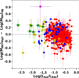
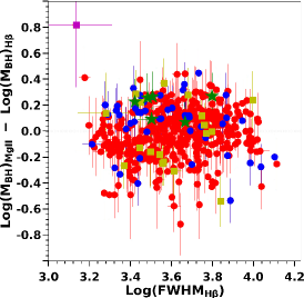
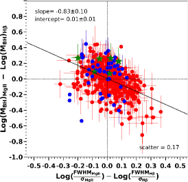
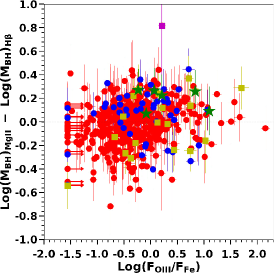
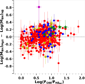
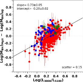
Figure 12.— Comparison of systematic difference between M_BH estimators from Mg II (Scheme 2) and H$\beta$ as a function of AGN parameters, i.e., Eddington ratio (top left), $\rm FWHM_{H\beta}$ (top middle), the difference of line profiles between H$\beta$ and Mg II (top right), F_OIII/F_FeII (bottom left), F_OIII/F_Hβ,narrow (bottom middle), L₃₀₀₀/L₅₁₀₀ (bottom right). The symbols are shown for the moderate-luminosity AGNs (blue), the SDSS sample (red), the 25 RM sources (yellow), the six HST targets (green), and NGC 4051 (pink). The best-fit slope is shown in thick black solid line. The dash-lines show different values of 0.

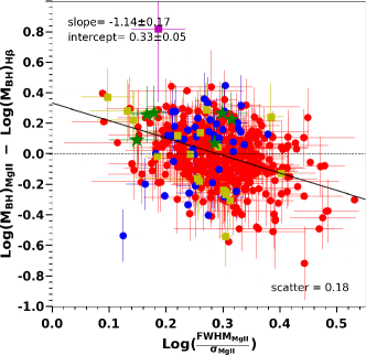
Figure 13.— Comparison of systematic difference between M_BH estimators from Mg II (Scheme 2) and H$\beta$ as a function of Mg II profile. The symbols are shown for the moderate-luminosity AGNs (blue), the SDSS sample (red), the 25 RM sources (yellow), the six HST targets (green), and NGC 4051 (pink). The best-fit slope is shown in thick black solid line. The dash-lines show different values of 0.

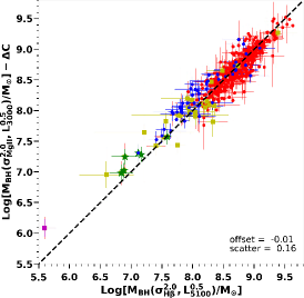
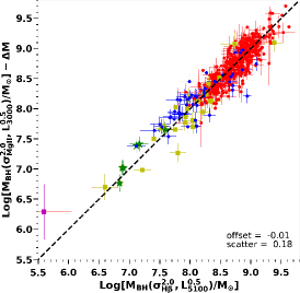
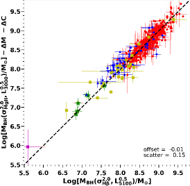
Figure 14.— Comparison of Mg II and H$\beta$-based based mass estimators after applying the correction term, $\rm\Delta C$ in Equation 12 (left panel), $\rm\Delta M$ in Equation 13 (middle panel) and the combination of the two terms (right panel). The symbols are shown for the moderate-luminosity AGNs (blue), the SDSS sample (red), the 25 RM sources (yellow), the six HST targets (green), and NGC 4051 (pink). The dash-lines show different values of 0.

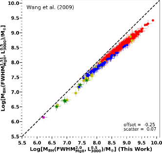
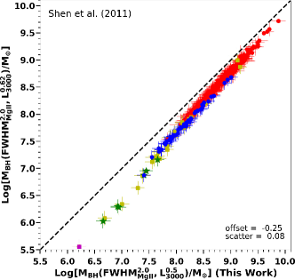
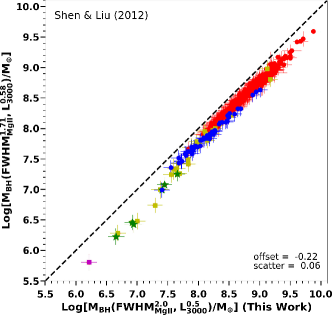
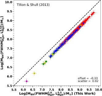
Figure 15.— Comparison of our M_BH calibration with various Mg II-based mass estimators e.g., Wang et al. (2009) (top left panel), Shen et al. (2011) (top right panel), Shen & Liu (2012) (bottom left panel), and Tilton & Shull (2013) (bottom right panel). The color schemes of sample are similar to those in Figure 7. The symbols are shown for the moderate-luminosity AGNs (blue), the SDSS sample (red), the 25 RM sources (yellow), the six HST targets (green), and NGC 4051 (pink). The dash-lines show different values of 0.

7. Conclusions

In this study, we present the calibration of M_BH estimators, using the combined sample of low, intermediate, and high luminosity AGNs with high quality spectra that have Mg II and H$\beta$ lines observed simultaneously. The dynamic range of $\mathrm{\lambda L_{5100}\sim 10^{41.3}-10^{46.5}}$ erg s^-1, and 5.5 $<$ $\log$M_BH $<$ 9.5 provides reliable mass estimators. We summarize the main results as follows:

(1) From the comparison of line width between the Mg II and H$\beta$ emission lines, $\sigma_{\rm MgII}$ and $\sigma_{\rm H\beta}$ show a linear relationship, while, FWHMs of both emission lines show a somewhat sub-linear relationship.

(2) Similar to our previous work, we found the linear relationship between the continuum luminosities of 3000Å and 5100Å. In addition, line luminosity of Mg II shows somewhat sub-linear relationship with that of H$\beta$, indicating the Baldwin effect in the UV range.

(3) In the case of the optical mass estimator, by using the fiducial mass from $\sigma_{\rm H\beta}$ and $\rm L_{5100}$, we obtained the H$\beta$-based M_BH estimator with a small intrinsic scatter $<$ 0.01 dex and rms scatter $<$ 0.13 dex. By using the reference mass from $\rm FWHM_{\rm H\beta}$ and $\rm L_{5100}$, we obtained an intrinsic scatter $<$ 0.12 dex and rms scatter $<$ 0.19 dex.

(4) Using the reference mass from $\sigma_{\rm H\beta}$ and $\rm L_{5100}$, we presented the Mg II M_BH estimator with the intrinsic scatter of 0.09$-$0.21 dex and rms scatter of 0.17$-$0.25 dex. With the reference mass from $\rm FWHM_{\rm H\beta}$ and $\rm L_{5100}$, we obtained an intrinsic scatter of 0.14$-$0.26 dex and rms scatter of 0.21$-$0.31 dex. In general, depending on the choice of line width ($\sigma$ or FWHM) and luminosity (emission line or continuum), we obtained different systematic uncertainties, i.e., rms scatter larger than $\sim$0.15 dex. Based on our calibrated estimators, $\sigma_{\rm MgII}$ and $\rm L_{3000}$ provide the best UV M_BH estimator with an intrinsic scatter of 0.09 dex and rms scatter of 0.17 dex.

(5) From the comparison of the systematic difference between the Mg II and H$\beta$-based M_BH estimators as a function of AGN properties, we found strong correlations between the UV and optical M_BH ratio and the ratio of line profiles of the Mg II and H$\beta$ lines and $\rm L_{5100}$/$\rm L_{3000}$. The discrepancy between Mg II and H$\beta$-based M_BH estimators is strongly dependent on the difference of line profiles between Mg II and H$\beta$. In addition, we suggested to add additional $\Delta$M correction factor (Equation 13) to reduce the systematic uncertainty between the UV and optical M_BH estimators.

Table 2 M_BH estimators based on Mg II, using the fiducial mass from $\sigma_{\rm H\beta}$ and $\rm L_{5100}$

Case	$\alpha$	$\beta$	$\gamma$	$\rm\sigma_{inst}$	$\rm\sigma_{rms}$		$\alpha$	$\beta$	$\gamma$	$\sigma_{inst}$	$\rm\sigma_{rms}$
(1)	(2)	(3)	(4)	(5)	(6)		(7)	(8)	(9)	(10)	(11)
			L3000 & $\sigma_{\rm MgII}$						L3000 & FWHMMgII
1) $\beta$ & $\gamma$ from scaling	7.54 $\pm$ 0.01	2.13 $\pm$ 0.06	0.54 $\pm$ 0.01	0.12 $\pm$ 0.01	0.20		6.92 $\pm$ 0.01	2.14 $\pm$ 0.07	0.54 $\pm$ 0.01	0.15 $\pm$ 0.01	0.20
2) $\beta$=2 & $\gamma$=0.5	7.61 $\pm$ 0.01	2.00	0.50	0.11 $\pm$ 0.01	0.19		7.04 $\pm$ 0.01	2.00	0.50	0.13 $\pm$ 0.01	0.19
3) $\beta$ = 2	7.57 $\pm$ 0.02	2.00	0.53 $\pm$ 0.02	0.11 $\pm$ 0.01	0.19		7.03 $\pm$ 0.02	2.00	0.51 $\pm$ 0.02	0.13 $\pm$ 0.01	0.19
4) $\gamma$=0.5	7.72 $\pm$ 0.02	1.51 $\pm$ 0.06	0.50	0.09 $\pm$ 0.01	0.17		7.35 $\pm$ 0.03	1.38 $\pm$ 0.05	0.50	0.10 $\pm$ 0.01	0.17
5) Free $\beta$ & $\gamma$	7.68 $\pm$ 0.02	1.49 $\pm$ 0.06	0.54	0.09 $\pm$ 0.01	0.17		7.33 $\pm$ 0.03	1.36 $\pm$ 0.06	0.53	0.10 $\pm$ 0.01	0.17
			LMgII & $\sigma_{\rm MgII}$						LMgII & FWHMMgII
1) $\beta$ & $\gamma$ from scaling	7.42 $\pm$ 0.01	2.13 $\pm$ 0.06	0.65 $\pm$ 0.01	0.20 $\pm$ 0.01	0.25		6.80 $\pm$ 0.01	2.14 $\pm$ 0.07	0.65 $\pm$ 0.01	0.21 $\pm$ 0.01	0.25
2) $\beta$=2 & $\gamma$=0.5	7.62 $\pm$ 0.01	2.00	0.50	0.18 $\pm$ 0.01	0.23		7.05 $\pm$ 0.01	2.00	0.50	0.18 $\pm$ 0.01	0.22
3) $\beta$ = 2	7.57 $\pm$ 0.03	2.00	0.54 $\pm$ 0.02	0.17 $\pm$ 0.01	0.23		7.03 $\pm$ 0.03	2.00	0.51 $\pm$ 0.02	0.18 $\pm$ 0.01	0.22
4) $\gamma$=0.5	7.80 $\pm$ 0.02	1.16 $\pm$ 0.07	0.50	0.14 $\pm$ 0.01	0.20		7.49 $\pm$ 0.03	1.12 $\pm$ 0.06	0.50	0.13 $\pm$ 0.01	0.19
5) Free $\beta$ & $\gamma$	7.72 $\pm$ 0.03	1.06 $\pm$ 0.07	0.59	0.13 $\pm$ 0.01	0.19		7.44 $\pm$ 0.03	1.03 $\pm$ 0.06	0.58	0.12 $\pm$ 0.01	0.18

Table 3 M_BH estimators based on Mg II, using the fiducial mass from $\rm FWHM_{H\beta}$ and $\rm L_{5100}$

Case	$\alpha$	$\beta$	$\gamma$	$\rm\sigma_{inst}$	$\rm\sigma_{rms}$		$\alpha$	$\beta$	$\gamma$	$\rm\sigma_{inst}$	$\rm\sigma_{rms}$
(1)	(2)	(3)	(4)	(5)	(6)		(7)	(8)	(9)	(10)	(11)
			L3000 & $\sigma_{\rm MgII}$						L3000 & FWHMMgII
1) $\beta$ & $\gamma$ from scaling	7.26 $\pm$ 0.01	3.20 $\pm$ 0.03	0.54 $\pm$ 0.01	0.17 $\pm$ 0.01	0.25		6.36 $\pm$ 0.01	3.17 $\pm$ 0.04	0.54 $\pm$ 0.01	0.20 $\pm$ 0.01	0.25
2) $\beta$=2 & $\gamma$=0.5	7.58 $\pm$ 0.01	2.00	0.50	0.16 $\pm$ 0.01	0.22		7.00 $\pm$ 0.01	2.00	0.50	0.16 $\pm$ 0.01	0.21
3) $\beta$ = 2	7.54 $\pm$ 0.03	2.00	0.53 $\pm$ 0.02	0.16 $\pm$ 0.01	0.22		6.99 $\pm$ 0.02	2.00	0.50 $\pm$ 0.02	0.16 $\pm$ 0.01	0.21
4) $\gamma$=0.5	7.47 $\pm$ 0.02	2.47 $\pm$ 0.08	0.50	0.15 $\pm$ 0.01	0.22		6.85 $\pm$ 0.04	2.30 $\pm$ 0.07	0.50	0.16 $\pm$ 0.01	0.21
5) Free $\beta$ & $\gamma$	7.44 $\pm$ 0.03	2.46 $\pm$ 0.08	0.53	0.14 $\pm$ 0.01	0.22		6.85 $\pm$ 0.04	2.30 $\pm$ 0.07	0.49	0.16 $\pm$ 0.01	0.21
			LMgII & $\sigma_{\rm MgII}$						LMgII & FWHMMgII
1) $\beta$ & $\gamma$ from scaling	7.14 $\pm$ 0.01	3.20 $\pm$ 0.03	0.65 $\pm$ 0.01	0.25 $\pm$ 0.01	0.31		6.24 $\pm$ 0.01	3.17 $\pm$ 0.04	0.65 $\pm$ 0.01	0.26 $\pm$ 0.01	0.30
2) $\beta$=2 & $\gamma$=0.5	7.58 $\pm$ 0.01	2.00	0.50	0.19 $\pm$ 0.01	0.25		7.00 $\pm$ 0.01	2.00	0.50	0.18 $\pm$ 0.01	0.23
3) $\beta$ = 2	7.51 $\pm$ 0.03	2.00	0.56 $\pm$ 0.02	0.19 $\pm$ 0.01	0.24		6.96 $\pm$ 0.03	2.00	0.54 $\pm$ 0.02	0.18 $\pm$ 0.01	0.22
4) $\gamma$=0.5	7.55 $\pm$ 0.02	2.13 $\pm$ 0.09	0.50	0.19 $\pm$ 0.01	0.25		6.98 $\pm$ 0.04	2.04 $\pm$ 0.07	0.50	0.18 $\pm$ 0.01	0.23
5) Free $\beta$ & $\gamma$	7.49 $\pm$ 0.03	2.07 $\pm$ 0.09	0.56	0.19 $\pm$ 0.01	0.24		6.95 $\pm$ 0.04	2.00 $\pm$ 0.07	0.54	0.18 $\pm$ 0.01	0.22

References

- Assef et al. (2011) Assef, R. J., Denney, K. D., Kochanek, C. S., et al. 2011, ApJ, 742, 93
- Bahk et al. (2019) Bahk, H., Woo, J.-H., Park, D. 2019, ApJ, 875, 50
- Baldwin (1977) Baldwin, J. A. 1977, ApJ, 214, 679
- Barth et al. (2011) Barth, A. J., Pancoast, A., Thorman, S. J., et al. 2011, ApJ, 743, L4
- Barth et al. (2015) Barth, A. J., Bennert, V. N., Canalizo, G., et al. 2015, ApJS, 217, 26
- Bennert et al. (2010) Bennert, V. N., Treu, T., Woo, J.-H., et al. 2010, ApJ, 708, 1507
- Bentz et al. (2006) Bentz, M. C., Peterson, B. M., Pogge, R. W., Vestergaard, M., & Onken, C. A. 2006, ApJ, 644, 133
- Bentz et al. (2009a) Bentz, M. C., Peterson, B. M., Netzer, H., Pogge, R. W., & Vestergaard, M. 2009, ApJ, 697, 160
- Bentz et al. (2009b) Bentz, M. C., Walsh, J. L., Barth, A. J. 2009, ApJ, 705, 199
- Bentz et al. (2013) Bentz, M. C., Denney, K. D., Grier, C. J., et al. 2013, ApJ, 767, 149
- Blandford & McKee (1982) Blandford, R. D., & McKee, C. F. 1982, ApJ, 255, 419
- Boroson & Green (1992) Boroson, T. A., & Green, R. F. 1992, ApJS, 80, 109
- Brotherton et al. (2015) Brotherton, M. S., Runnoe, J. C., Shang, Z., & DiPompeo, M. A. 2015, MNRAS, 451, 1290
- Bruzual & Charlot (2003) Bruzual, G., & Charlot, S. 2003, MNRAS, 344, 1000
- Cackett et al. (2015) Cackett, E. M., Gültekin, K., Bentz, M. C., et al. 2015, ApJ, 810, 86
- Cho et al. (2020) Cho, H., Woo, J.-H., Hodges-Kluck, E., et al. 2020, ApJ, 892, 93
- Clavel et al. (1991) Clavel, J., et al. 1991, ApJ, 366, 64
- Collin et al. (2006) Collin, S., Kawaguchi, T., Peterson, B. M., & Vestergaard, M. 2006, A&A, 456, 75
- Coatman et al. (2017) Coatman, L., Hewett, P. C., Banerji, M., et al. 2017, MNRAS, 465, 2120
- Denney et al. (2009) Denney, K. D., Peterson, B. M., Dietrich, M., Vestergaard, M., & Bentz, M. C. 2009, ApJ, 692, 246
- Denney (2012) Denney, K. D. 2012, ApJ, 759, 44
- Dietrich & Kollatschny (1995) Dietrich, M., & Kollatschny, W. 1995, A&A, 303, 405
- Dong et al. (2009) Dong, X.-B., Wang, T.-G., Wang, J.-G., et al. 2009, ApJ, 703, L1
- Du et al. (2016) Du, P., Lu, K.-X., Zhang, Z.-X., et al. 2016, ApJ, 825, 126
- Du et al. (2017) Du, P., Zhang, Z.-X., Wang, K., et al. 2018, ApJ, 856, 6
- Du & Wang (2019) Du, P. & Wang, J.-M., ApJ, 886, 42D
- Ferrarese & Merrit (2000) Ferrarese, L., & Merritt, D. 2000, ApJ, 539, L9
- Fausnaugh (2017) Fausnaugh, M. M. 2017, PASP, 129, 024007
- Gebhardt et al. (2000) Gebhardt, K., Bender, R., Bower, G., et al. 2000, ApJ, 539, L13
- Grandi (1982) Grandi, S. A. 1982, ApJ, 255, 25
- Greene & Ho (2005) Greene, J. E., & Ho, L. C. 2005, ApJ, 630, 122
- Grier et al. (2013) Grier, C. J., Martini, P., Watson, L. C., et al. 2013, ApJ, 773, 90
- Grier et al. (2017) Grier, C. J., Trump, J. R., Shen, Y., et al. 2017, ApJ, 851, 21
- Grier et al. (2019) Grier, C. J., Shen, Y., Horne, K., et al. 2019, ApJ, 887, 38
- Ho et al. (1995) Ho, L. C., Filippenko, A. V., & Sargent, L. W. 1995, ApJS, 98, 477
- Karouzos et al. (2015) Karouzos, M., Woo, J.-H., Matsuoka, K., et al. 2015, ApJ, 815, 128
- Kaspi et al. (2000) Kaspi, S., Smith, P. S., Netzer, H., et al. 2000, ApJ, 533, 631
- Kaspi et al. (2005) Kaspi, S., Maoz, D., Netzer, H., et al. 2005, ApJ, 629, 61
- Kormendy & Ho (2013) Kormendy, J., & Ho, L. C. 2013, ARA&A, 51, 511
- Kong et al. (2006) Kong, M. Z., Wu, X. B., Wang, R., & Han, J. L. 2006, CHJAA, 396, 410
- Kovačević-Dojčinović et al. (2017) Kovačević-Dojčinović, J., Marčeta-Mandić, S., & Popović, L. Č. 2017, arXiv:1707.08251
- Le et al. (2014) Le, H. A. N., Pak, S., Im, M., et al. 2014, JASR, 54, 6
- Le & Woo (2019) Le, H. A. N. & Woo, J-.H. 2019, ApJ, 887, 246
- Lira et al. (2018) Lira, P., Kaspi, S., Netzer, H. 2018, ApJ, 865, 56L
- Malkan et al. (2017) Malkan, M. A., Jensen, L. D., Rodriguez, D. R., Spinoglio, L., & Rush, B. 2017, ApJ, 846, 102
- Malkan & Sargent (1982) Malkan, M. A., & Sargent, W. L. W. 1982, ApJ, 254, 22
- Markwardt (2009) Markwardt, C. B. 2009, in Astronomical Data Analysis Software and Systems XVIII, ed. D. A. Bohlender, D. Durand, & P. Dowler (San Francisco: ASP), 251
- Marziani et al. (2013) Marziani, P., Sulentic, J. W., Plauchu-Frayn, I., & del Olmo, A. 2013, A&A, 555, A89
- Mejia-Restrepo et al. (2016) Mejia-Restrepo, J. E., Trakhtenbrot, B., Lira, P., Netzer, H., & Capellupo, D. M., MNRAS, 187, 211
- McGill et al. (2008) McGill, K. L., Woo, J.-H., Treu, T., & Malkan, M. A. 2008, ApJ, 673, 703
- McLure & Dunlop (2004) McLure, R. J., & Dunlop, J. S. 2004, MNRAS, 352, 1390
- McLure & Jarvis (2002) McLure, R. J., & Jarvis, M. J. 2002, MNRAS, 337, 109
- Metzroth et al. (2006) Metzroth, K. G., Onken, C. A., & Peterson, B. M. 2006, ApJ, 647, 901
- Moustakas et al. (2006) Moustakas, J., & Kennicutt, R. C., Jr. 2006, ApJS, 164, 81
- Oke et al. (1995) Oke, J. B., Cohen, J. G., Carr, M., et al. 1995, PASP, 107, 375
- Onken et al. (2004) Onken, C. A., Ferrarese, L., Merritt, D., et al. 2004, ApJ, 615, 645
- Pancoast et al. (2014) Pancoast, A., Brewer, B. J., Treu, T., et al. 2014, MNRAS, 445, 3073
- Park et al. (2012a) Park, D., Woo, J.-H., Treu, T., et al. 2012a, ApJ, 747, 30
- Park et al. (2012b) Park, D., Kelly, B. C., Woo, J.-H., & Treu, T. 2012b, ApJ, 203, 6
- Park et al. (2013) Park, D., Woo, J.-H., Denney, K. D., & Shin, J. 2013, ApJ, 770, 87
- Park et al. (2015) Park, D., Woo, J.-H., Bennert, V. et al. 2015, ApJ, 799, 164
- Park et al. (2017) Park, S., Woo, J.-H., Romero-Colmenero, E., et al. 2017, ApJ, 847, 125
- Peterson (1993) Peterson, B. M. 1993, PASP, 105, 247
- Peterson et al. (2004) Peterson, B. M., Ferrarese, L., Gilbert, K. M., et al. 2004, ApJ, 613, 682
- Peterson (2007) Peterson, B. M. 2007, in ASP Conf. Ser. 373, The Central Engine of Active Galactic Nuclei, ed. L. C. Ho & J.-W. Wang (San Francisco, CA: ASP), 3
- Rafiee & Hall (2011) Rafiee, A. & Hall, P. B. 2011, ApJS, 194, 42
- Rakshit et al. (2019) Rakshit, S., Woo, J.-H., Gallo, E. 2019, ApJ, 886, 93
- Reichert et al. (1994) Reichert, G. A., Rodriguez-Pascual, P. M., Alloin, D., et al. 1994, ApJ, 425, 582
- Runnoe et al. (2013) Runnoe, J. C., Brotherton, M. S., Shang, Z., & DiPompeo, M. A. 2013a, MNRAS, 434, 848
- Salviander et al. (2007) Salviander, S., Shields, G. A., Gebhardt, K., & Bonning, E. W. 2007, ApJ, 662, 131
- Schlegel et al. (1998) Schlegel, D. J., Finkbeiner, D. P., & Davis, M. 1998, ApJ, 500, 525
- Shankar et al. (2016) Shankar, F., Bernardi, M., Sheth, R. K., et al. 2016, MNRAS, 460, 3119
- Shankar et al. (2019) Shankar, F., Weinberg, D. H., Marsden, C. et al. 2019, MNRAS, 493, 1500
- Shen et al. (2011) Shen, Y., Richards, G. T., Strauss, M. A., et al. 2011, ApJS, 194, 45
- Shen & Liu (2012) Shen, Y., & Liu, X. 2012, ApJ, 753, 125
- Shen & Ho (2014) Shen, Y., & Ho, L. C. 2014, Nature, 513, 210
- Shen et al. (2016) Shen, Y., Horne, K., Grier, C. J., et al. 2016, ApJ, 818, 30
- Shin et al. (2019) Shin, J., Nagao, T., Woo, J. -H., & Le, H. A. N. 2019, ApJ, 874, 1
- Sulentic et al. (2012) Sulentic, J. W., Marziani, P., Zamfir, S., & Meadows, A. 2012, ApJL, 752, L7
- Sun et al. (2015) Sun, M., Trump, J. R., Brandt, W. N., et al. 2015, ApJ, 802, 14
- Sun et al. (2018) Sun, M., Xue, Y., Richards, G. T., et al. 2018, ApJ, 854, 128S
- Tilton & Shull (2013) Tilton, E. T., & Shull, J. M. 2013, ApJ, 774,67
- Trakhtenbrot & Netzer (2012) Trakhtenbrot, B., & Netzer, H. 2012, MNRAS, 427, 3081
- Tremaine et al. (2002) Tremaine, S., Gebhardt, K., Bender, R., et al. 2002, ApJ, 547, 2
- Treu et al. (2004) Treu, T., Malkan, M. A., & Blandford, R. D. 2004, ApJ, 615, L97
- Tsuzuki et al. (2006) Tsuzuki, Y., Kawara, K., Yoshii, Y., et al. 2006, ApJ, 650, 57
- Valdes et al. (2004) Valdes, F., Gupta, R., Rose, J. A., Singh, H. P., & Bell, D. J. 2004, ApJS, 152, 251
- Vanden Berk et al. (2001) Vanden Berk, D. E., Richards, G. T., Bauer, A., et al. 2001, AJ, 122, 549
- Vestergaard (2002) Vestergaard, M. 2002, ApJ, 571, 733
- Vestergaard & Peterson (2006) Vestergaard, M., & Peterson, B. M. 2006, ApJ, 641, 689
- Vestergaard & Wilkes (2001) Vestergaard, M., & Wilkes, B. J. 2001, ApJS, 134, 1
- Wandel et al. (1999) Wandel, A., Peterson, B. M., & Malkan, M. A. 1999, ApJ, 526, 579
- Vanden Berk et al. (2001) Vanden Berk, D. E., Richards, G. T., Bauer, A., et al. 2001, AJ, 122, 549
- Wang et al. (2009) Wang, J.-G., Dong, X.-B., Wang, T.-G., et al. 2009, ApJ, 707, 1334
- Wang et al. (2019) Wang, S., Shen, Y., Jiang, L., et al. 2019, ApJ, 882, 1
- Wolf et al. (2019) Wolf, J., Salvato, M., Coffey, D., et al. 2019, arXiv: 191101947v1
- Woo & Urry (2002) Woo, J.-H., & Urry, C. M. 2002, ApJ, 579, 530
- Woo et al. (2006) Woo, J.-H., Treu, T., Malkan, M. A., & Blandford, R. D. 2006, ApJ, 645, 900
- Woo (2008) Woo, J.-H. 2008, AJ, 135, 1849
- Woo et al. (2010) Woo, J.-H., Treu, T., Barth, A. J., et al. 2010, ApJ, 716, 269
- Woo et al. (2013) Woo, J.-H., Schulze, A., Park, D., et al. 2013, ApJ, 772, 49
- Woo et al. (2015) Woo, J.-H., Yoon, Y., Park, S. et al. 2015, ApJ, 801, 38
- Woo et al. (2016) Woo, J.-H., Bae, H.-J., Son, D., & Karouzos, M. 2016, ApJ, 817, 108
- Woo et al. (2018) Woo, J.-H., Le, H. A. N., Karouzos, M., et al. 2018, ApJ, 859, 138
- Woo et al. (2019a) Woo, J,-H., Son, D., Gallo, E., et al. 2019, arXiv:1907.00771
- Woo et al. (2019b) Woo, J.-H., Cho, H., Gallo, E., et al. 2019, Nature Astronomy, 3, 755
- Xue et al. (2010) Xue, Y. Q., Brandt, W. N., Luo, B., et al. 2010, ApJ, 720, 368
- Xue (2017) Xue, Y. Q. 2017, NewAR, 79, 59
- Zheng & Malkan (1993) Zheng, W., & Malkan, M. A. 1993, ApJ, 415, 517
- Zhu et al. (2017) Zhu, D., Sun, M., & Wang, T. 2017, ApJ, 843, 30