Can Smartphone Co-locations Detect Friendship? It Depends How You Model It.

Abstract.

We present a study to detect friendship, its strength, and its change from smartphone location data collected among members of a fraternity. We extract a rich set of co-location features and build classifiers that detect friendships and close friendship at 30% above a random baseline. We design cross-validation schema to test our model performance in specific application settings, finding it robust to seeing new dyads and to temporal variance.

1. Introduction

Friendship is a “voluntary, personal relationship typically providing intimacy and assistance”, associated with characteristics of trust, loyalty, and self-disclosure (Fehr, 1996). It is one of the most important aspects of human existence, lending meaning to life, and providing for material, cognitive, and social-emotional needs in ways that lead to greater health and well-being (Fehr, 1996).

Understanding the friendship relationship between people can be helpful for creating technology that serves people better. If an individual’s friendships are known, these can be leveraged for applications supporting help-seeking behavior such as requests for recommendations or for favors, or for automatically establishing trust between users’ devices. Friendships may also be leveraged for carrying out social interventions around diet and exercise (Madan et al., 2010b) or for preventing disease transmission (Madan et al., 2010a), such as in mobile applications that facilitate friends adopting and holding each other accountable to healthy behaviors. Conversely, it may be of interest to create applications to make recommendations about friendships in order to help bring people together, for example at conferences (Chin et al., 2012, 2013) or for information dissemination in workplaces (Lawrence et al., 2006). Longitudinal information about changes in friendships could help detect the onset of isolation and help design interventions to strengthen friendships.

But in order to incorporate information about one’s friendship network in personal informatics and mobile applications, we need ways of detecting friendship. One easy way to get ‘ground truth’ is to rely on ties from online social networking platforms; but such ties are not necessarily good proxies for the underlying construct of friendship (Wilson et al., 2012; Corten, 2012; Mislove et al., 2007). Survey instruments have been the standard network data collection method in social network analysis for decades, but involve a high burden for users that make them impractical as a basis for mobile applications.

Previous social science work has established the strong link between individuals being physically close and being friends (Festinger et al., 1950; Fehr, 1996; Latané et al., 1995). There is a two-way causal connection in that people who spend time together are more likely to become friends (Festinger et al., 1950), and that people who are friends spend time together (Fehr, 1996). This suggests that there should be a robust signal of friendship in measurements of physical proximity that can then be leveraged for analysis, services, or interventions.

Our work is the first effort to detect friendships using feature extraction from smartphone location data. Previous works either descriptively, rather than predictively, linked location data and friendship (Eagle et al., 2009), looked at ties on location-based online social network services (Cranshaw et al., 2010), or used mobile phone call and SMS logs (Wiese et al., 2014, 2015). We believe that detecting friendship from mobile phone co-location data is a realistic approach for future mobile applications and interventions that seek to leverage friendship for other tasks.

This paper presents the results of a 3-month study of a cohort of 53 participants, with final analysis performed on 9 weeks of data from 48 participants. We combine mobile phone sensor data collection with established social network survey instruments, and use rich feature extraction from co-location data to see how well such data can be used to detect friendships, close friendships, and changes in friendship.

Our contributions are as follows:

• We present, to our knowledge, the first pairwise feature extraction from smartphone location data, and show that a classifier built with the extracted features performs 30% above random (Matthews correlation coefficient). This can serve as a baseline for all future work.

• We design a novel evaluation method (using temporal block assignment cross-validation and what we call dyadic assignment cross-validation ) to mimic different realistic application settings in order to more rigorously test our classification’s generalizability to these settings, and use it to show that our approach is robust to seeing new pairings of individuals, and to variability in co-location patterns over time.

Below, first we review background work in social network analysis and in the mobile and pervasive computing literature around existing approaches to extracting interactions and/or friendships from mobile sensor data. We describe our study design, and our feature extraction process. With extracted features, we build a predictive model and use feature importance as a step towards characterizing the aspects of co-location most useful for detecting friendship.

2. Background and related work

2.1. Friendship ties

Friendship is an example of a relational phenomenon. Relational phenomena are two-unit or dyadic relations (Borgatti et al., 2009). Instead of the $n$ individuals of a dataset being the observations, they have as observations $\binom{n}{2}$ undirected (symmetric) relations (e.g., co-location), or $2\times\binom{n}{2}$ directed (potentially asymmetric) relations (e.g., self-reported friendships) between individuals.

Research throughout the 20th century has provided examples of friendship and other ties having explanatory and predictive power, such as in explaining why girls ran away from a school for delinquent teenage girls and predicting future runaways (Moreno, 1934), explaining the breakup of a monastery (Sampson, 1968), of the split of a karate club into two separate clubs (Zachary, 1977), or using structures of informal networks to predict the success or failure of institutional reorganization (Krackhardt, 1996). Insights from these approaches have proved robust as they have been successfully integrated into search engines, recommender systems, and the structure of social media platforms.

We represent a collection of friendship ties between $n$ people as an $n\times n$ adjacency matrix, $A$, where

$$A_{ij}=\begin{cases}1\mbox{ if there is a tie }i\to j\\ 0\mbox{ otherwise.}\end{cases}$$

and where $A_{ii}=0$ (no self-loops). $A$ is not necessarily symmetric, as friendship ties collected from sources like surveys can and do yield cases of $A_{ij}\neq A_{ji}$. As an (asymmetric) adjacency matrix defines a (directed) graph, which in this case is a friendship network, we refer to the $n$ people as nodes. We refer to an (unordered) pair of individuals $(i,j)$ as a dyad, and a value where $A_{ij}=1$ as an edge, and also interchangeably as a tie or link.

While $A_{ij}$ represents a ‘dependency’ between units $i$ and $j$, for example $A_{ij}=1$ will frequently be associated with similar outcomes from $i$ and $j$, such ties are themselves dependent (Snijders, 2011). For example, while friendship ties are not necessarily mutual or reciprocated, we still have $A_{ij}=A_{ji}$ more often than we would expect at random. In symbolic terms, $P(A_{ij})\centernot{\mathchoice{\mathrel{\hbox to0.0pt{$\displaystyle\perp$\hss}\mkern 2.0mu{\displaystyle\perp}}}{\mathrel{\hbox to0.0pt{$\textstyle\perp$\hss}\mkern 2.0mu{\textstyle\perp}}}{\mathrel{\hbox to0.0pt{$\scriptstyle\perp$\hss}\mkern 2.0mu{\scriptstyle\perp}}}{\mathrel{\hbox to0.0pt{$\scriptscriptstyle\perp$\hss}\mkern 2.0mu{\scriptscriptstyle\perp}}}}P(A_{ji})$

Other such dependencies include transitivity, which are friend-of-a-friend connections, $P(A_{ij})\centernot{\mathchoice{\mathrel{\hbox to0.0pt{$\displaystyle\perp$\hss}\mkern 2.0mu{\displaystyle\perp}}}{\mathrel{\hbox to0.0pt{$\textstyle\perp$\hss}\mkern 2.0mu{\textstyle\perp}}}{\mathrel{\hbox to0.0pt{$\scriptstyle\perp$\hss}\mkern 2.0mu{\scriptstyle\perp}}}{\mathrel{\hbox to0.0pt{$\scriptscriptstyle\perp$\hss}\mkern 2.0mu{\scriptscriptstyle\perp}}}}P(\{A_{ik},A_{kj}:k\neq i,j\})$, and preferential attachment (Perc, 2014), $P(A_{ij}\centernot{\mathchoice{\mathrel{\hbox to0.0pt{$\displaystyle\perp$\hss}\mkern 2.0mu{\displaystyle\perp}}}{\mathrel{\hbox to0.0pt{$\textstyle\perp$\hss}\mkern 2.0mu{\textstyle\perp}}}{\mathrel{\hbox to0.0pt{$\scriptstyle\perp$\hss}\mkern 2.0mu{\scriptstyle\perp}}}{\mathrel{\hbox to0.0pt{$\scriptscriptstyle\perp$\hss}\mkern 2.0mu{\scriptscriptstyle\perp}}}}P(\{A_{kj}:k\neq j\})$.

Not accounting for such dependencies can, in explanatory models, lead to too-small standard errors and omitted variable bias (Dow et al., 1982, 1984; Dow, 2007). In predictive models (Shmueli, 2010; Breiman, 2001), dyadic dependencies impact the validity of cross-validation estimates of model performance (Dabbs and Junker, 2016) in ways similar the impacts of other types of dependencies (Hammerla and Plötz, 2015).

For example, if $A_{ij}=A_{ji}$, for co-location features $X_{ij}$, if the pair $(A_{ij},X_{ij})$ is in the training set and $(A_{ji},X_{ij})$ is in the test set, we would be training and testing on the exact same row of data!

In any link prediction task, having a cross-validation scheme that does not reflect an application setting (for example, using features related to network degree or to the number of mutual friends when we may not have the complete network) can potentially give a misleading picture of what true out-of-sample performance would be.

To avoid these problems, we first avoid using features that would not be available in an application settings (network features, lagged values of the class label, etc.). We also employ three different cross-validation schemes, described below. There are existing methods for doing cross validation with network data (Chen and Lei, 2017; Dabbs and Junker, 2016), but their validity depends on strong assumptions and even then they do not control for all known dependencies; instead, by employing different cross validation schema, we get a better picture of how our classifier would work in different use cases.

2.2. Friendship and co-location

The connection of friendship and proximity has long been a topic of study in social science. In a foundational work of social psychology carried out in 1946, the ‘Westgate study’, Festinger et al. (Festinger et al., 1950) carried out a field experiment around soldiers returning from WWII and attending graduate school at MIT on the GI bill. They and their families were randomly placed into the units of the relatively isolated, newly built Westgate housing complex. The study authors were able to quantify the extent to which people living close by, or passing one another on the way to their residences, were more likely to become friends than with others with whom they did not have opportunities for interaction (although the study looking only at men may have neglected an important causal process in the role of women, (Cherry, 1995)). Then, in 1954 and 1955, the ‘Newcomb-Nordlie fraternity’ study (Nordlie, 1958; Newcomb, 1961) recruited two waves of 17 male students who did not know each other, gave them free ‘fraternity-style’ housing, and studied how their personal characteristics, political positions, and interests affected their eventual friendship formation. These two studies established that proximity plays an important role in friendship, but also that proximity is not sufficient, and that other characteristics matter.

Later work (Latané et al., 1995) further quantified the relationship between distance and friendship, finding “the inverse square of the distance separating two persons” to be a good fit to measures of social impact. A retreat for all incoming sociology majors at the University of Groningen provided another opportunity for studying the emergence of friendship, with van Duijn et al. (van Duijn et al., 2003) finding that friendships developed due to one of four main effects: physical proximity, visible similarity, invisible similarity, and network opportunity.

There are also a number of studies using data from online social networks or other online platforms to study the connection between friendship and geography, although many of these are at the global scale (Liben-Nowell et al., 2005; Quercia et al., 2012; Leskovec and Horvitz, 2014; Cho et al., 2011; Backstrom et al., 2010) and do not have resolution at the scales at which interactions can occur. Furthermore, users of location-based social networks, or those who share locations on general online social networks like Twitter and Facebook, are a fraction of total users and form an unrepresentative sample (Malik et al., 2015) for a general smartphone-using population. Other work has taken call logs and used calls as the ties to study with respect to geography (Onnela et al., 2011; Wang et al., 2011), although call logs and SMS have a surprisingly poor relationship with friendship as measured by self-report (Wiese et al., 2014, 2015).

A landmark series of papers by Bernard, Killworth, and Sailer (Killworth and Bernard, 1976, 1979; Bernard and Killworth, 1977; Bernard et al., 1979, 1982) showed that people are generally bad at recalling objective patterns of interaction. However, subsequent work (Freeman et al., 1987; Krackhardt, 1987) argued that psychological perceptions of the network, rather than objectively measurable ties of interaction, were causal for individuals’ behavior: subjective data may in some cases be more valuable for predicting and explaining, and thus the psychological perceptions captured by survey data may be more valuable for certain tasks than objective measurements.

This is related to adams’ [sic] (adams, 2010) critique of the model in Eagle et al. (Eagle et al., 2009) predicting friendship from co-location; adams notes that there are ‘close strangers and distant friends’, both of which a method based on co-location would misclassify. In response, Eagle et al. (Eagle et al., 2010) argue that some causal network processes might happen unconsciously, and sensor measurements might be able to detect these. The correlation of friendship and proximity can make it difficult to sort out which may be causal for a given process (Cohen-Cole and Fletcher, 2008). But in the future, if we can decorrelate friendships and proximity by controlling for one or the other, it could help us understand whether social influence or environmental factors are more likely to be the causal factor. Furthermore, for many mobile use cases, even imperfect friendship detection will be relevant, making the task of friendship detection from co-location a worthwhile pursuit.

2.3. Sensors for social networks

Since the first work with the ‘sociometer’ (later, ‘sociometric badge’) in 2002 (Choudhury and Pentland, 2002), research groups have been using sensors to collect data about social interactions. Studies often used sensor ‘nodes’ or other custom devices (Paradiso et al., 2010; Angelopoulos et al., 2011; Förster et al., 2012; Friggeri et al., 2011; Hsieh et al., 2010; Laibowitz et al., 2006) and, with the exception of RFID tags (Barrat et al., 2013), studies have largely used mobile devices (Stopczynski et al., 2014, 2015; Kiukkonen et al., 2010; Rachuri et al., 2011; Li et al., 2012; Do and Gatica-Perez, 2011; Eagle and Pentland, 2006; Raento et al., 2009; Kjærgaard and Nurmi, 2012; Lawrence et al., 2006; Sekara and Lehmann, 2014, 2014) because of their wide range of existing sensors, and because their use results in lower participant burden than when participants are required to wear or carry an additional device. The data used is either co-location data (from either GPS, self-reported check-ins, or mutual detection of fixed sensors or WiFi hotspots) or proximity (through Bluetooth or RFID). There are also studies that use video to detect interactions (Chen et al., 2007; Ke et al., 2013; Kong and Fu, 2016; van Gemeren et al., 2016), and sociometric badges (Choudhury and Pentland, 2002) or headsets (Madan and Pentland, 2006) that gather audio data that allows for detecting conversations between specific individuals, but, in our work, we focus on the co-location and proximity sensing made possible with mobile phones.

These existing studies largely fall into three categories. Most common are studies that describe infrastructure, technical details, and study design, followed sometimes by descriptive modeling of network characteristics and some bivariate relationships (Stopczynski et al., 2014, 2015; Sekara and Lehmann, 2014, 2014; Kiukkonen et al., 2010; Li et al., 2012; Lepri et al., 2012; Choudhury and Pentland, 2003a, b; Chronis et al., 2009; Angelopoulos et al., 2011; Aharony et al., 2011; Barrat et al., 2008; Cattuto et al., 2010; Barrat et al., 2012, 2013; Förster et al., 2012; Friggeri et al., 2011; Isella et al., 2011; Miklas et al., 2007; Rachuri et al., 2011). This has been important work that has contributed to present-day mobile sensing tools – tools that are capable of going beyond exploration and overall descriptives into measuring specific processes, and applications designed on top of those processes like network-based health interventions (Madan et al., 2010a).

The second category is of those that try to build systems other than the specific sensing platform. They may build or lay the groundwork for recommender systems (Chin et al., 2012, 2013; Ganti et al., 2008; Lawrence et al., 2006), or present models or algorithms for mining information about interactions from sensor data (Do and Gatica-Perez, 2011, 2013; Eagle and Pentland, 2006; Phung et al., 2008).

The third category is of those that employ statistical models or techniques to make conclusions or predictions using sensor data. Stehlé et al. (Stehlé et al., 2013) look at the connection between ‘spatial behavior’, measured by RFID badges, and gender similarity. The ‘Friends and Family’ or ‘SocialfMRI’ study and dataset (Aharony et al., 2011) has been used to look at the connection between interaction and financial status (Pan et al., 2011) and interaction and sleep and mood (Moturu et al., 2011). Madan et al. (Madan et al., 2011) used sensor measurements to look at the relationship between social interactions and changes in political opinion. The ‘Reality Mining’ dataset (Eagle and Pentland, 2006) has similarly been used to look at obesity and exercise in the presence of contact between people (Madan et al., 2010b). Another approach is that of Eagle & Pentland (Eagle and Pentland, 2009), which presents a spectral clustering system for extracting daily patterns from time series. Staiano et al. (Staiano et al., 2012) use ego networks (induced subgraphs of single nodes and all their respective neighbors) in call logs, Bluetooth-based proximity networks, and surveys to predict Big-5 personality traits.

In this third category, and most similar to our work, are two papers based on the Reality Mining dataset (Dong et al., 2011; Eagle et al., 2009). Eagle and Pentland (Eagle et al., 2009) were the first to use mobile phone data proximity to infer a network of self-reported friendship ties. They first calculated a ‘probability of proximity’ score over the range of a week as an average frequency of proximity over nine months of data, which they showed was systematically different for each of reciprocated self-reported ties $(A_{ij},A_{ji})=(1,1)$, non-reciprocated ties $(A_{ij},A_{ji})\in\{(0,1),(1,0)\}$, and no ties $(A_{ij},A_{ji})=(0,0)$. But their model did not use cross-validation, and their findings were based on aggregating over nine months of data to model a friendship self-report from the first month, which does not match a mobile use case which would involve detecting friendships only from recently gathered batches of location data.

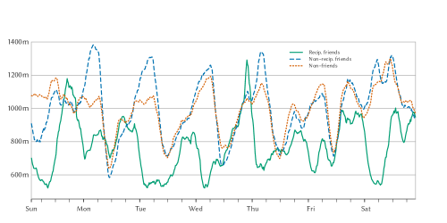
Figure 3. The median weekly pairwise distances between reciprocated (mutual) friendships, $A_{ij}=A_{ji}=1$, non-reciprocated friendships, $A_{ij}=1\neq A_{ji}=0$ or $A_{ij}=0\neq A_{ji}=1$, and non-friendships, $A_{ij}=A_{ji}=0$, for times when pairs are within the area of the university, and aggregated over the entire period of data (i.e., no training/test split). This is analogous to the approach of (Eagle et al., 2009), and this figure reproduces their figure 2 (except with median distance, rather than mean frequency of proximity). While it appears there is a strong pattern, it is a result of an aggregation that obscures the variance between weeks and in data splitting, such that this seeming pattern proved ineffective as a basis of classification in testing.

We explored replicating their approach; while we also found that, when aggregated over the entire time period of data collection, there was a major difference between mutual friendship ties and both non-ties and non-reciprocated ties (fig. 3), this pattern proved ineffective for building a classifier because of how aggregation like this, over time, dyads, and splits of training and test sets, obscures the variance that poses challenges to good test performance.

Dong et al. (Dong et al., 2011) also modeled the co-evolution of behavior and social relationships from mobile phone sensor data. They outlined a model that predicted self-reported friendships from sensor data (and other survey data), but also did not use cross-validation, and only reported one performance metric: that the binomial model explained 22% of overall variance, of which 6% was due to sensor data. This presumably from a pseudo R-squared metric, but as the specific metric is not given and there was no cross-validated performance reported, it is difficult to compare results.

We now describe the questions we seek to answer and the study and analysis we conducted to answer them.

3. Study design and procedure

The goal of our study is to understand the feasibility of inferring social relationships (friendship in particular) from (only) passive smartphone data. We are especially interested in the following questions:

1. How well can we detect friendships from co-location features? In other words, if all we know about two people in a social system is their location patterns, how accurately can we say if they are friends?

2. If we know that friendships exist, how well can we detect if these friendships are close friendships?

3. How accurately can we detect whether a friendship is likely to change? Will co-location patterns provide information about the creation or dissolution of friendships?

To answer these questions, we carried out a 3-month study among members of a fraternity to use smartphone data to try and capture interactions and relationships as they were formed and evolved during that period. The following section describes the study setup and data collection process.

3.1. Participants and recruitment

We recruited members of an undergraduate fraternity in a research university in the northeastern United States. The fraternity had 60 members at the start of the study, with an additional 21 prospective members going through the ‘pledging’ process during the study duration, of which 19 completed the process. Of this cohort of 79 men, we recruited 66 participants, of which 53 ultimately participated in sensor data collection, and of which 48 responded to at least one survey wave. Having this sort of well-defined boundary specification (Laumann et al., 1983) let us ask each study participant about their friendships with each member of the fraternity, giving negative examples that are explicit, unlike open-ended solicitation for friendships (such as from ‘name generator’ instruments) in which individuals are only implicitly not friends by not being mentioned.

The fraternity was relatively loose-knit; about 20 fraternity members live in a fraternity house, with the rest living elsewhere and required to be in the fraternity only one day a week (for a fraternity chapter-wide meeting). Participants were compensated $20 a week for having the passive and automated sensor data collection software, AWARE (Ferreira et al., 2015), installed on their smartphones, with additional $5 incentives for each survey wave they completed.

3.2. Data collection

Our task was to use mobile phone sensor data relating to location and proximity in a model that could recover self-reported friendship ties, and changes in such ties. Consequently, we collected survey data about friendships in three waves, and used AWARE to collect Wifi, Bluetooth, and location data from mobile phones.

3.2.1. Survey data

During the study, participants were asked to fill out a survey asking about their social connections, based off of existing instruments (Knecht et al., 2010; van de Bunt et al., 1999). There was a public listing of fraternity members, and consequently we were able to ask about respondents’ ties to all fraternity members (i.e., ask about ties to everybody in the specified boundary), not just those participating in the study; while we were not able to relate friendships with non-participant fraternity members to sensor data, since non-participation meant we do not have sensor data, it does give a sense of the importance of non-participants in the social system.

The surveys were collected three times over 9 weeks: shortly after the beginning of the study, then four weeks after, and lastly at the end of the study five weeks later (we made the second period longer, as one of these five weeks was spring break, when many study participants were away from campus). Participants were asked about five different quantities: their recollections about who they interacted with frequently; who they considered to be a friend; who they considered to be a close friend; who they went to for advice on personal matters; and who they went to for advice on professional/academic matters. The correlation between these collected networks, between each other and over time, is given below in figure (4). Friendship can change at shorter intervals than six weeks; but since friendship is an internal and subjective psychological construct, currently the only way of getting data on friendship is surveys with high respondent burden that makes it infeasible to collect at more frequent intervals.

3.2.2. Passive smartphone data

We equipped each participant with the AWARE mobile phone framework (Ferreira et al., 2015) on their iOS devices ($\approx$90% of participants) or Android devices (the remaining $\approx$10%). There were no users of Windows or other mobile operating systems. We used AWARE to record Bluetooth and WiFi detections, each at 10 minute sampling intervals. We also had continuous monitoring of battery and screen status (on/off), and complete records of call and message metadata (with hashed values for phone numbers). For location, the Android AWARE client uses the Google fused location plugin, which has several options for trading off accuracy and battery usage, and for which we selected the low power option. The iOS AWARE client uses the iOS location services, in which we similarly selected an option with low battery usage.

We also performed WiFi fingerprinting in the fraternity house to help us determine when participants were co-located in rooms in the house.

4. Data processing

4.1. Data Handling

4.1.1. Survey data

The completeness of the survey data is shown in figure (1a). The response rate dropped in each survey round; compared to survey 1, survey 2 had a response rate of 59%, and survey 3 had a response rate of 51%. In total, there were 48 participants providing network data, 34 of which responded to 2 surveys giving us longitudinal network data (the minimum requirement for detecting changes in friendship), including 20 participants that responded to all 3 surveys. In total, out of $\binom{48}{2}=1128$ potential pairs, we were able to train and/or test on $830$ pairs.

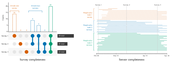
Figure 1. (a. Left) Looking at longitudinal completeness, 14 people completed survey 1 only, and none completed surveys 2 or 3 only. 9 people completed surveys 1 and 2, 5 people completed surveys 1 and 3, none completed 2 and 3 only, and 20 people completed all three waves. This is shown in the vertical bars at the top. This comes out to 48 respondents for survey 1, 29 respondents for survey 2, and 25 respondents for survey 3, shown in the solid horizontal bars on the right side. (b. Right) We show the time periods in which sensor data was collected for people who answered one survey (dotted lines), two surveys (dashed lines), or all three surveys (solid lines). The times of the three surveys are marked with vertical lines.

4.1.2. Sensor data

The completeness of the sensor data is shown in figure (1b). Some logistical problems prevented all participants from starting smartphone data collection on the first day, and some participants discontinued the use of the app because of technical issues (battery life, sporadic interference with certain external Bluetooth devices, etc.).

There were two sources of missing values in the calculated features: either artifacts relating to no observations fulfilling a certain criteria (e.g., no co-locations within 50m on mornings), or else actual missing data (one or both mobile devices were not providing a certain sensor’s data during a given period, e.g., mornings of a given week). For the former (artifacts), we replaced missing values with appropriate substitutes, such as 0s or the maximum possible value. For logarithmic features, some of which could be less than 1, we replaced $-\infty$ with zeros. For inverse-squared features, we replaced $\infty$ with a value, 200, slightly larger than the largest observed inverse-squared value.

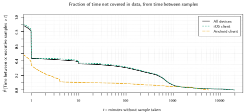
Figure 2. A plot of the survival function (the empirical complementary cumulative distribution) for time not covered by sensor data. 40% of the study time across all participants is covered by sensor readings less frequent than 10 minutes, meaning that 60% of the data has no gaps in coverage.

Based on the distribution of lengths of time where data was missing (fig. 2), we would have needed to interpolate up to eight hour intervals to have any real impact on the proportion of time that has missing data. Consequently, we chose to not use partial interpolation, and kept cells of missing values in the feature matrix. This necessitated using classifiers that can handle missing values among the features, like the R random forest implementation rpart (Therneau and Atkinson, 2018) which has procedures for handling missing values when constructing decision trees, and other packages built on top of rpart.

We did test our assumptions about the importance of maintaining missing values by trying different variations. We did try out last value carried forward interpolation on the time series prior to feature extraction, as well as mean, median, and mode interpolation on the matrix of extracted features, but neither improved results.

4.1.3. Spring break

Spring break may be extremely informative, for example if two people are proximate to each other but far from everybody else it may be that they are more likely to be friends. However, spring break is systematically different from every other week, such that if we train on spring break, we have no meaningful test set. Thus, we removed spring break from the data set. This is also why the two periods have an unequal number of weeks, with 4 weeks between survey waves 1 and 2, and 5 weeks between survey waves 2 and 3; spring break fell between survey waves 2 and 3, such that removing it leaves 4 weeks in each period.

4.2. Collected surveys and sensors

4.2.1. Network survey instrument

We asked participants about five different types of ties in each of the three surveys: following previous social science literature, we asked about advice-seeking relationships (both personal advice seeking, and academic/professional advice-seeking), in addition to asking about friendships and, for each reported friendship, asking if it was also a close friendship. For comparison with work on recall (Bernard and Killworth, 1977; Bernard et al., 1979, 1982; Killworth and Bernard, 1976, 1979) and memorability of social interactions (Latané et al., 1995), we also asked about frequency of interaction.

The similarities between these collected networks, both for the same network across the three waves and between the different networks, is given in figure (4). The similarity metric used is the Jaccard index, a common method for comparing networks (as it looks only at ties shared across the two networks, not shared non-ties), potentially of overlapping but unequal sets of nodes, which in our case happens because of non-response. For two networks $N_{A}$ and $N_{B}$, with $n_{A\cap B}$ overlapping nodes and adjacency matrices $A$ and $B$ restricted to these nodes, the Jaccard index is

$$J(A,B)=\frac{|\{A_{ij}=B_{ij}=1\}|}{2\times\binom{n_{A\cap B}}{2}}$$

As we can see, there is a much higher correlation between self-reported frequent interaction and friendship than there is between friendship and close friendship. There is also a high correlation between close friendship and the two types of advice ties; while we did not use advice ties in the current analysis, this similarity gives insight into what types of relationships the prompt about ‘close friendships’ elicit (like the prompt about friendship, we explicitly do not define what we mean by ‘close’, letting participants interpret the term).

Looking at the changes in the networks from survey to survey, we see that close friendships and both types of advice-seeking relationships are much less variable over time than are friendships or self-reports of frequent interaction.

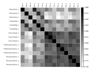
Figure 4. The similarity between networks (5 types of ties, each collected 3 times), measured via the Jaccard index. The self-reported frequent interaction and friendship networks are more similar than the other networks, and both also exhibit more variation across the three waves.

4.2.2. Bluetooth

Collected Bluetooth data turned out to be unusable. Both Android and iOS no longer make the 16 hex digit Bluetooth MAC addresses of detected devices available to app developers. Instead, detected devices are recorded in terms of a 32 hex digit universally unique identifier (UUID), which are assigned by the detecting device uniquely to each detected device and used to recognize those detected devices in the future.

4.2.3. Call logs and SMS

Following the findings of Wiese et al. (Wiese et al., 2014, 2015) that call logs and SMS do not necessarily help detect degree of friendships, we elected to restrict our attention to using co-location only. Another reason to avoid call logs and SMS are that such communications metadata are already seen as sensitive and intrusive, even if they were to turn out to not help us predict our target of interest. Lastly, there was a substantive reason to not use communications data: we were informed that the fraternity largely used a group chat application for communications with one another, such that we expected call logs and SMS to not capture any informative aspects of communications.

4.2.4. Wifi

One candidate for characterizing proximity is when two devices detect or connect to the same Wifi device. Here, Wifi hotspot MAC addresses are unique (unlike the hotspot name/label, which for example with ‘eduroam’ is shared not only across multiple hotspots in the same university, but across multiple cities across the world!), and mutual detection of this picks up when two devices are proximate. Out of 830 potential pairs, 406 pairs of mobile devices detected at least one Wifi hotspot in common (although not necessarily at the same time).

As mentioned above, we also conduced Wifi fingerprinting in the fraternity house, including collecting all Wifi devices detected in each room along with the received signal strength indication (RSSI) of the respective signals. In order to perform Wifi fingerprinting (match a set of hotspots that are detected by a mobile phone in a given scan and with respective RSSIs to previously collected profiles from specific rooms), we needed multiple detected hotspots per scan (every 10 minutes). However, we found that only about 6.7% of scans for Wifi hotspots recorded more than one detected hotspot; in the frat house as well, we could tell when a device was connected to one of the frat house’s Wifi hotspots, but not which other hotspots were detected in order to determine a specific room. Thus, we only use as the basis for features whether at least one Wifi hotspot was detected in common at the scan of a specific 10 minute interval from two devices, ignoring the tiny fraction of detections that include multiple devices, and also ignoring RSSI. The frat house has 5 main Wifi devices for about 30 rooms over 3 floors. Based on the size of rooms in the fraternity house and the relative coverage of its Wifi devices, we estimate that at least within the fraternity house, our Wifi localization approach is accurate to within a bit of a smaller radius than its general 32m accuracy, perhaps 20m or so; however, we do not have similar measurements for the rest of campus.

4.2.5. Location

Since we have, from previous theory, that co-location is causally related to friendship through interaction, we would ideally want to extract features from pairwise distance measurements that will be effective as a proxy for interaction. However, in the Google Fused Location plugin that AWARE uses to collect location data, we used the PRIORITY_LOW_POWER option which prioritizes low power usage, as previous testing with AWARE had showed battery drain was a major cause of participant dropout. This low power option does not actively use GPS, instead using a combination of cell phone towers and detected Wifi hotspot with known geolocations, and is advertised as being accurate to within about 10km. In the iOS client, the accuracy setting corresponding to low power use was to set desiredAccuracy option to 1km, with a threshhold for recording new movements of 1000m. In practice, the reported accuracy was usually much better, with a significant portion of readings reporting an accuracy of within 10m.

Additionally, when calculating the continuous-valued time series of pairwise distances, we also generated binary time series for if the locations of both members of the pair fell within a geobox around the university’s campus, and a geobox around the fraternity house.

As a way of reducing the continuous-valued time series, we sought to pick several choice thresholds that might characterize geographic similarity in simple way. First, we plot an empirical complementary cumulative distribution function (i.e., a survival function) in log-$x$ scale (fig. 5a) to see the overall distribution. There is an ‘elbow’ around 2000m, which is about the size of the university and surrounding area. Then, within 2000m, we use 1-dimensional clustering (Wang et al., 2011), weighted by time and using 10 clusters, and used the boundaries of the fitted clusters as thresholds. These thresholds are shown as the boundaries regions of gray over a kernel density estimate of the distribution over the first 2000m (fig. 5b).

Figure 5. A survival function (a. left), plotted in log-$x$ scale, shows pairwise distances over time. Based on the ‘elbow’ around 2000m (approximately the size of the university and surrounding area), marked with a vertical dotted line, we only found clusters for pairwise distances below 2000m. Below 2000m, we clustered distances (again weighted by the time spent at that distance). The fitted clusters are shown on top of a kernel density estimate (b. right) that gives a detail of the head of the distribution. The cluster breaks are at 207m, 422m, 626m, 822m, 1001m, 1178m, 1373m, 1570m, 1776m, and then our cutoff of 2000m. These are also listed in table (1).

After data processing, we have the following:

• 1 continuous-valued time series of pairwise distances

• 10 binary time series of whether both members of a given pair were within a given threshold of each other

• 1 binary time series of whether both members of a given pair were within a geobox around the university campus

• 1 binary time series of whether both members of a given pair were within a geobox around the fraternity house

• 1 binary time series of whether both members of a given pair detected at least one Wifi hotspot in common

• 1 binary time series of whether both members of a given pair detected a Wifi hotspot visible from the fraternity house in common

Next, to compare self-reported ties and co-location, it is necessary to summarize these time series into a set of features. These are summarized in table (1).

Table 1. Extracted features. “$\otimes$” indicates taking all pairwise combinations. The thresholds are irregularly spaced because they are empirically derived from 1-dimensional clustering; see figure (5b) for these clusters.

For the continuous time series and each of the binary time series, we extract relevant summary statistics relating to central tendency, variance, and (if applicable) range. We employed summaries of distributions after logarithmic transformation after observing that the original distributions were often heavily right-skewed. Additionally, for the binary time series, we can consider the length of sequences of consecutive 1s (spans of co-location at the given threshold) and of consecutive 0s (gaps between co-location at the given threshold). These are integer-valued but we treat them as continuous, and calculate an additional set of summary statistics accordingly. All of these summary statistics are given in the central column of table (1).

Lastly, each of these feature types are crossed with time periods: weekdays only and weekends only, nights only (12am - 6am), mornings only (6am - 12pm), afternoons only (12pm - 6pm), and evenings only (6pm - 12am). These are shown in the right column of table (1).

In total, there are $9$ features for the continuous-valued time series of pairwise distances, $12\times(5+20)=300$ features for the binary time series, and each of these 309 features are calculated over seven settings, for $309\times 7=2163$ candidate location features. Wifi features were $2\times(5+20)=50$, and $50\times 7=350$ for an additional 350 features, for a total of 2,513 features. We extracted these over two 4-week periods, corresponding to the 4 weeks between surveys 1 and 2, and the 5 weeks between surveys 2 and 3 with the week of spring break subtracted out.

5. Modeling targets and evaluation methods

5.1. Modeling targets

We take on three targets for modeling.

1. Detecting friendship. This is a standard binary classification task. In this task, we do not make use of survey wave 1.

2. Detecting friendship strength. Given that two people are friends, can we detect whether or not they have reported that the friendship is a close one? For this, we restrict the data set to instances of friendship ties only, and do binary classification of close friendships. Again, we do not make use of survey wave 1.

3. Detecting change in friendship. Here, our targets are

   • $P(A_{ij}^{(t)}=A_{ij}^{(t+1)}\mid X^{[t,t+1)})$: No change in friendship (either no friendship, or maintained friendship)

   • $P(A_{ij}^{(t)}\neq A_{ij}^{(t+1)}\mid X^{[t,t+1)})$: Change in friendship (either tie creation or tie dissolution)

   While we ideally would be able to separately model tie creation and dissolution, as they are distinct processes (Snijders et al., 2010), in our data only a small proportion of ties changed in either direction such that modeling became difficult. We will see below that this modeling target was the most challenging of all, although treating it as a multiclass problem over the direction of change only led to worse performance.

5.2. Cross-validation schema

In order to comprehensively evaluate our classifier’s performance at detecting friendship, we use three cross-validation schema. Each corresponds to a different use case, and tests the generalizability of our method to that use case. In each case, dependencies (redundancies in data, latent or unmodeled similarities) between training and test sets can share information across a split in data, dependencies that would not be present in application settings, therefore inflating test performance compared to real-world performance.

Each schema uses a different rule and use case to assign observations to training and test folds. The rules and use cases of these schema are detailed below.

5.2.1. Cross validation with unrestricted assignment

This is independently assigning each observed $A_{ij}$ to a fold. It corresponds to a use case where a model is trained on a population ($n-k$ pairs) and then applied back to $k$ pairs from same population (potentially seeing the same people multiple times, or the same dyad in multiple directions).

5.2.2. Cross validation with dyadic assignment

This groups all values associated with a pair of individuals (a dyad), that is, $(A_{ij}^{(1)},A_{ji}^{(1)},A_{ij}^{(2)},A_{ji}^{(2)},A_{ij}^{(3)},A_{ji}^{(3)})$, and assign the entire 6-tuple to a single fold. Some values in the tuple will be missing, causing folds to be of different sizes; But since assignment to fold is not dependent of the number of missing values, sizes will be the same in expectation.

Such assignment controls for reciprocity and temporal autocorrelation. For reciprocity, if $A_{ij}=A_{ji}$, then the label-feature pair $(A_{ij},X_{ij})$ and $(A_{ji},X_{ji})$ are identical and should not be split between training and test. Similarly for temporal autocorrelation, if two people’s friendship and co-location patterns do not change over time, then $(A_{ij}^{(t)},X_{ij}^{[t-1,t)})$ and $(A_{ij}^{(t+1)},X_{ij}^{[t,t+1)})$ would also be very similar and should not be split between training and test.

Cross validation with dyadic assignment corresponds to a use case where we have not previously seen the labeled co-location patterns of a given dyad, whether previously in time or in one direction, to have included it as a training instance.

5.2.3. Cross validation with temporal block assignment

This splits data by whether a class label is from survey 2 or survey 3 (for detecting friendship and strength of friendship) or is the change from survey 1 to 2 or the change from survey 2 to 3 (for detecting change in friendship). In other words, for detecting friendship and strength, we train on $(A^{(2)},X^{[1,2)})$ and test on $(A^{(3)},X^{[2,3)})$, and for detecting change, we train on $(A^{(1)},A^{(2)},X^{[1,2)})$ and test on $(A^{(2)},A^{(3)},X^{[2,3)})$.

As a note, here we can only split into 2 folds as we only have two observation spans between different surveys. Cross validation with temporal block (Bergmeir and Benítez, 2012; Racine, 2000) assignment accounts for temporal variation in co-location. If there is a great deal of variability in co-location patterns, then our classifier would have little generalizability over time. In this case, if we train with instances with features from both $X^{[t-1,t)}$ and $X^{[t,t+1)}$, it would even out the temporal variation and obscure the lack of generalizability. But if we train only on instances associated with features $X^{[t-1,t)}$ and then test only on instances associated with features $X^{[t,t+1)}$, it simulates how well out classifier will do in predicting friendships from future patterns of co-location data.

5.3. Evaluation metric

To summarize classifier performance, we rely on the Matthews correlation coefficient (MCC). This is the same as Pearson’s $\phi$, or mean square contingency coefficient, an analog for a pair of binary variables of Pearson’s product-moment correlation coefficient, but was rediscovered by Matthews (Matthews, 1975) for use as a classification metric. For the count of true positives (TP), true negatives (TN), false positives (FP) and false negatives (FN), the MCC is

$$\text{MCC}=\frac{TP\times TN-FP\times FN}{\sqrt{(FP+TP)\times(TP+FN)\times(TN+FP)\times(TN+FN)}}.$$

The MCC has several desirable properties. First, like the F1 score and area under the ROC curve (AUC), it summarizes the performance on both classes in a single number. Unlike AUC and F1, however, it has an interpretable range: 0 for random predictions, -1 for perfect misclassification, and 1 for perfect classification. Most helpfully, is a good summary of performance in cases of class imbalance (Boughorbel et al., 2017), which have here (about a 25:75 split). We include other metrics, but rely on the MCC as the single-number summary of how far we are above a random baseline of MCC = 0. Note that, if we predict the majority class for all instances, the MCC is also zero.

5.4. Feature Selection

Feature selection can often improve classifier performance, but it is also useful for diagnostic and exploratory analysis. In our case, we are interested in a reduced set of features that can provide similar or better classification results, and that may be less burdensome to extract for use in real-time mobile applications built on friendship detection. To produce a selected set of features, we use Correlation-based Feature Selection (CFS) (Hall, 1999), which selects features that are both correlated with the class label, and uncorrelated with one another.

To select the most stable set of features, we run the CFS method on the training set built with what turns out to be our most conservative cross validation scheme, temporal block assignment. We take the half of data with features extracted from the first four weeks and further divide it into 10 folds. We perform CFS of each fold, then look at the features that were selected in the maximum number of folds, an approach also applied more formally elsewhere (Meinshausen and Bühlmann, 2010).

We choose those features that appeared in CFS runs on at least 9 of the 10 folds. These features are then entered in the classification process for friendship detection.

6. Results

6.1. Friendship detection

Results for the three cross-validation schemes are given in table (2). In each case, the no information rate corresponds to the proportion of the majority class, 0, and would be the accuracy we would get if we always predicted no tie.

The unrestricted assignment gives better results than either of the other two CV schema, showing that labeling a previously unseen dyad is indeed a more specific and difficult task than what is evaluated by unrestricted assignment, and that there is a significant amount of variation in co-location patterns over time—and that while our classifier performance does drop, it still generalizes across patterns in time.

We use a one-sided binomial test of the accuracy against the No Information Rate (NIR), equal to the frequency of the majority class, and find that both unrestricted and dyadic CV are significant at the usual $p<0.05$ level. Under temporal block CV, the classifier is only significantly better than the NIR at the $p<0.1$ level.

In our classifications, the MCC ranges from .30 in CV with unrestricted assignment, to .26 in CV with dyadic assignment, and .21 in CV with temporal block assignment. This indicates that the classifier performance is between 30% and 21% better than baseline (for which MCC=$0$).

Cross validation	Unrestricted	Dyadic	Temporal block
Accuracy	0.8006	0.7920	0.7913
Accuracy, 95% CI	(0.7882, 0.8125)	(0.7794, 0.8042)	(0.7726, 0.8091)
(No Information Rate / Majority class)	(0.7740)	(0.7740)	(0.7785)
Binomial test, Accuracy vs. NIR, $p$-value	$p$=1.5e-05	$p$=0.0025	$p$=0.0901
Precision (Positive predictive value)	0.6918	0.6508	0.6812
Recall/Sensitivity (True positive rate)	0.2122	0.1723	0.1088
Specificity (True negative rate)	0.9724	0.9730	0.9855
F1 score	0.3248	0.2724	0.2964
AUC	0.7148	0.7039	0.1876
Matthews correlation coefficient	0.3039	0.2562	0.2120

Table 2. Friendship detection, test performance across the three CV schema. The no information rate corresponds to a baseline accuracy given by predicting no ties; in the case of networks, this is 1 minus the density of the network.

6.2. Detecting close friendships

We repeat the assessment of the above models, conditioning on the presence of a friendship, and making our detection target whether or not a friendship is reported to be close. In this case, the network of close friendships has a network density of .41, making the no information rate .59.

Cross validation	Unrestricted	Dyadic	Temporal block
Accuracy	0.6817	0.6670	0.5741
Accuracy, 95% CI	(0.6511, 0.7112)	(0.6361, 0.6969)	(0.5259, 0.6212)
(No Information Rate / Majority class)	(0.5861)	(0.5861)	(0.5185)
Binomial test, Accuracy vs. NIR, $p$-value	$p$=7.6e-10	$p$=1.8e-07	$p$=0.0117
Precision (Positive predictive value)	0.6904	0.6711	0.7069
Recall/Sensitivity (True positive rate)	0.4188	0.3832	0.1971
Specificity (True negative rate)	0.8674	0.8674	0.9241
F1 score	0.5213	0.4879	0.3083
AUC	0.6997	0.6695	0.5889
Matthews correlation coefficient	0.3250	0.2906	0.1777

Table 3. Close friendship detection, conditioned on the presence of a friendship, test performance across the three CV schema.

We see a similar pattern of performance, with temporal block CV being the most conservative (18% better than baseline), and unrestricted CV being more optimistic (32% better than baseline).

6.3. Detecting changes in friendship

Detecting loss in friendships could be particularly important for social interventions, such as preventing the onset of isolation. However, the rarity of changes in friendship (only 13% of ties change, either being created or dissolving) complicates modeling.

Our approach in meaningfully detect changes in friendship proved to be challenging. AdaBoost failed to predict any positive test cases for any CV schema; a random forest performed better with a Matthews correlation coefficient of .07 for the unrestricted CV and .03 for the dyadic-based CV (see table (4). The classifier output does not pass a statistical test for being significantly better than the No Information Rate. One of the reasons for the poor performance may be the type of features used in the classification. We used the same aggregated features used for friendship detection to detect change. However, change in friendship may be reflected in the feature values and thus a feature set that contains change values may better capture change in friendship.

Cross validation	Unrestricted	Dyadic
Accuracy	0.6842	0.8645
Accuracy, 95% CI	(0.6692, 0.6989)	(0.8532, 0.8752)
(No Information Rate / Majority class)	(0.8710)	(0.8710)
Binomial test, Accuracy vs. NIR, $p$-value	$p$=1	$p$=0.8902
Precision (Positive predictive value)	0.1676	0.2093
Recall/Sensitivity (True positive rate)	0.3651	0.0183
Specificity (True negative rate)	0.7315	0.9898
F1 score	0.2297	0.0336
AUC	0.5483	0.5167
Matthews correlation coefficient	0.0720	0.0256

Table 4. Change detection, random forest test performance. AdaBoost made only negative test classifications, but random forests (performance shown here) did make some positive classifications under unrestricted and dyad-based CV, although under temporal block CV again there were no positive classifications.

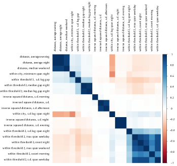
Figure 6. Correlations between the features selected via CFS on the training set of a temporal block cross-validation scheme. The ordering is from the angular order of eigenvectors.

Feature	Distribution	Summary statistic	Timeframe
1.	Distance	Mean	Evening
2.	Distance	Mean	Night
3.	Distance	Median	Weekend
4.	Within city	Minimum span	Night
5.	Within threshold 3	Log gap	All
6.	Within threshold 2	Median gap	Night
7.	Within threshold 2	Median log gap	Night
8.	Inverse squared distance	S.D.	Morning
9.	Inverse squared distance	S.D.	All
10.	Inverse squared distance	S.D.	Afternoon
11.	Within city	S.D. log span	Night
12.	Inverse squared distance	Standard deviation	Night
13.	Inverse squared distance	Standard deviation	Evening
14.	Within threshold 2	S.D. log span	Night
15.	Within threshold 2	Max span	Night
16.	Within threshold 2	Count	Night
17.	Within threshold 2	Max span	Weekend
18.	Within threshold 2	Count	Morning
19.	Within threshold 2	S.D. span	Weekday

Table 5. The 19 features selected via CFS on the training set from temporal block assignment: what they measure, how they summarize it, and the timeframe in which they summarize it. Ordering is from angular order of eigenvectors on the correlation matrix (fig. 6).

6.4. Feature Selection

While we applied CFS to select features from the training set in all tasks, the features selected were not always consistent across folds, and across cross validation schema. So, we focus on the features selected in the case of the most conservative cross validation schema, and the extent to which feature selection improved model performance here.

Applying CFS to only the training data from temporal block assignment and splitting it into 10 folds, we find 19 features that are selected in 9 or 10 of the folds. Using only these features leads to improved test performance from temporal block assignment, shown in table (6), which also includes the test performance with this set of features under each cross validation scheme.

CV assignment method	Unrestricted	Dyadic	Temporal block
Accuracy	0.7975	0.793	0.7923
Accuracy, 95% CI	(0.785, 0.8095)	(0.7804, 0.8051)	(0.7736, 0.8101)
(No Information Rate / Majority class)	(0.774)	(0.774)	(0.7785)
Binomial test, Accuracy vs. NIR, $p$-value	$p$=0.0001	$p$=0.0016	$p$=0.0734
Precision (Positive predictive value)	0.6602	0.6370	0.5799
Recall/Sensitivity (True positive rate)	0.2143	0.1954	0.2269
Specificity (True negative rate)	0.9678	0.9675	0.9532
F1 score	0.3236	0.2990	0.3261
AUC	0.6837	0.6804	0.6767
Matthews correlation coefficient	0.2921	0.2682	0.2658

Table 6. Friendship detection with CFS feature selection on the temporal block assignment training data.

While the test MCC of CV with unrestricted assignment goes down, with this fraction of only 19 features the test MCC of CV with dyadic assignment rises slightly, and the test MCC of CV with temporal block assignment does far better, going from an MCC of .21 to .27. These 19 features, then, seem to be picking up a significant portion of the pattern in co-location data, and a pattern that is more robust to changes over time.

While it is dangerous to substantively interpret the selected features as causal or even as necessarily stable (Mullainathan and Spiess, 2017; Yang and Yang, 2016), it is a useful exploratory step to see the features that are effective for the detection task. The features are listed in table (5) ,with the pairwise correlations given in figure (6). While there are groups of highly linearly correlated features, many of the features are not correlated, giving an independent signal.

There are some patterns that emerge in this well-performing subset of features. Threshold 2 (422m) shows up frequently, as do measures related to variance (standard deviation measures), nighttime, and the distribution of inverse squared distances. This generates several hypotheses: first, that Latané et al.’s (Latané et al., 1995) finding that inverse-squared distance fits well to reports of memorable social interactions may be effective for friendship detection as well. Second, the threshold at 422m seems particularly relevant versus others: this specific value might not be what is important, but perhaps this captures some relevant radius around the frat house. Otherwise, features associated with where people are co-located at night appear most frequently, which is in contrast to the finding by Eagle et al. (Eagle et al., 2009) that the daytime probability proximity is what was discriminative for friendships.

7. Conclusion and Future Work

In this paper, we have described the collection of subjective, self-reported friendship data alongside objective sensor data within a given boundary specification. We modeled friendship, close friendships, and change in friendship with machine learning and evaluated them using three cross-validation schema that accounted for different use case scenarios in the real world to show the generalizability of our approach. We could detect friendship and close friendship with a significant better performance above baseline in both cases. Our change detection, however, performed poorly with current aggregated features, suggesting a different set of features are needed to carry out this task.

We also obtained a set of features through a CFS method on the most conservative training set (one constructed through temporal block assignment). Our test using the extracted features showed similar results to the full feature set, suggesting them as potential alternatives to the full feature set that can help building lightweight models, and suggesting that certain measures and timeframes, such as inverse squared distance, standard deviations, and nighttime patterns, are most helpful for detection. In our future work, we will further explore feature selection for a parsimonious set of features applicable for different detection tasks.

Our findings demonstrate the feasibility of detecting friendships from location data, as well as establish the challenge of detecting changes in friendship. This opens possibilities for further investigating the relationship between friendship and co-location, as well as for designing mobile applications that build recommendation systems or interventions based on detected friendships.

References

- (1)
- adams (2010) jimi adams. 2010. Distant friends, close strangers? Inferring friendships from behavior. Proceedings of the National Academy of Sciences 107, 9 (2010), E29–E30. https://doi.org/10.1073/pnas.0911195107
- Aharony et al. (2011) Nadav Aharony, Wei Pan, Cory Ip, Inas Khayal, and Alex Pentland. 2011. Social fMRI: Investigating and shaping social mechanisms in the real world. Pervasive and Mobile Computing 7, 6 (2011), 643–659. https://doi.org/10.1016/j.pmcj.2011.09.004
- Angelopoulos et al. (2011) Constantinos Marios Angelopoulos, Christofoulos Mouskos, and Sotiris Nikoletseas. 2011. Social signal processing: Detecting human interactions using wireless sensor networks. In Proceedings of the 9th ACM International Symposium on Mobility Management and Wireless Access (MobiWac ’11). 171–174. https://doi.org/10.1145/2069131.2069163
- Backstrom et al. (2010) Lars Backstrom, Eric Sun, and Cameron Marlow. 2010. Find me if you can: Improving geographical prediction with social and spatial proximity. In Proceedings of the 19th International Conference on World Wide Web (WWW ’10). 61–70. https://doi.org/10.1145/1772690.1772698
- Barrat et al. (2013) Alain Barrat, Ciro Cattuto, Vittoria Colizza, Francesco Gesualdo, Lorenzo Isella, Elisabetta Pandolfi, Jean-François Pinton, Lucilla Ravà, Caterina Rizzo, Mariateresa Romano, Juliette Stehlé, Alberto Eugenio Tozzi, and Wouter van den Broeck. 2013. Empirical temporal networks of face-to-face human interactions. The European Physical Journal Special Topics 222, 6 (2013), 1295–1309. https://doi.org/10.1140/epjst/e2013-01927-7
- Barrat et al. (2012) Alain Barrat, Ciro Cattuto, Vittoria Colizza, Lorenzo Isella, Caterina Rizzo, Alberto Eugenio Tozzi, and Wouter van den Broeck. 2012. Wearable sensor networks for measuring face-to-face contact patterns in healthcare settings. In Revised Selected Papers from the Third International Conference on Electronic Healthcare (eHealth 2010, Vol. 69). 192–195. https://doi.org/10.1007/978-3-642-23635-8_24
- Barrat et al. (2008) Alain Barrat, Ciro Cattuto, Vittoria Colizza, Jean-François Pinton, Wouter Van den Broeck, and Alessandro Vespignani. 2008. High resolution dynamical mapping of social interactions with active RFID. arXiv:0811.4170. arXiv:https://arxiv.org/abs/0811.4170
- Bergmeir and Benítez (2012) Christoph Bergmeir and José M. Benítez. 2012. On the use of cross-validation for time series predictor evaluation. Information Sciences 191 (2012), 1920–213. https://doi.org/10.1016/j.ins.2011.12.028
- Bernard and Killworth (1977) H. Russell Bernard and Peter D. Killworth. 1977. Information accuracy in social network data II. Human Communication Research 4, 1 (1977), 3–18. https://doi.org/10.1111/j.1468-2958.1977.tb00591.x
- Bernard et al. (1979) H. Russell Bernard, Peter D. Killworth, and Lee Sailer. 1979. Informant accuracy in social network data IV: A comparison of clique-level structure in behavioral and cognitive network data. Social Networks 2, 3 (1979), 191–218. https://doi.org/10.1016/0378-8733(79)90014-5
- Bernard et al. (1982) H. Russell Bernard, Peter D. Killworth, and Lee Sailer. 1982. Informant accuracy in social-network data V: An experimental attempt to predict actual communication from recall data. Social Science Research 11, 1 (1982), 30–66. https://doi.org/10.1016/0049-089X(82)90006-0
- Borgatti et al. (2009) Stephen P. Borgatti, Ajay Mehra, Daniel J. Brass, and Giuseppe Labianca. 2009. Network analysis in the social sciences. Science 323, 5916 (2009), 892–895. https://doi.org/10.1126/science.1165821
- Boughorbel et al. (2017) Sabri Boughorbel, Fethi Jarray, and Mohammed El-Anbari. 2017. Optimal classifier for imbalanced data using Matthews Correlation Coefficient metric. PLOS ONE 12, 6 (06 2017), 1–17. https://doi.org/10.1371/journal.pone.0177678
- Breiman (2001) Leo Breiman. 2001. Statistical modeling: The two cultures (with comments and a rejoinder by the author). Statistical Science 16, 3 (08 2001), 199–231. https://doi.org/10.1214/ss/1009213726
- Cattuto et al. (2010) Ciro Cattuto, Wouter van den Broeck, Alain Barrat, Vittoria Colizza, Jean-François Pinton, and Alessandro Vespignani. 2010. Dynamics of person-to-person interactions from distributed RFID sensor networks. PLOS ONE 5, 7 (2010), e11596. https://doi.org/10.1371/journal.pone.0011596
- Chen et al. (2007) Datong Chen, Jie Yang, Robert Malkin, and Howard D. Wactlar. 2007. Detecting social interactions of the elderly in a nursing home environment. ACM Transactions on Multimedia Computing, Communications, and Applications 3, 1 (2007). https://doi.org/10.1145/1198302.1198308
- Chen and Lei (2017) Kehui Chen and Jing Lei. 2017. Network cross-validation for determining the number of communities in network data. J. Amer. Statist. Assoc. (2017), 1–11. https://doi.org/10.1080/01621459.2016.1246365
- Cherry (1995) Frances Cherry. 1995. One man’s social psychology is another woman’s social history. In The stubborn particulars of social psychology: Essays on the research process. Routledge, London, 68–83.
- Chin et al. (2013) Alvin Chin, Bin Xu, Hao Wang, Lele Chang, Hao Wang, and Lijun Zhu. 2013. Connecting people through physical proximity and physical resources at a conference. ACM Transactions on Intelligent System Technologies 4, 3 (2013), 50:1–50:21. https://doi.org/10.1145/2483669.2483683
- Chin et al. (2012) Alvin Chin, Bin Xu, Hao Wang, and Xia Wang. 2012. Linking people through physical proximity in a conference. In Proceedings of the 3rd International Workshop on Modeling Social Media (MSM ’12). 13–20. https://doi.org/10.1145/2310057.2310061
- Cho et al. (2011) Eunjoon Cho, Seth A. Myers, and Jure Leskovec. 2011. Friendship and mobility: User movement in location-based social networks. In Proceedings of the 17th ACM SIGKDD international conference on Knowledge discovery and data mining (KDD ’11). 1082–1090. https://doi.org/10.1145/2020408.2020579
- Choudhury and Pentland (2002) Tanzeem Choudhury and Alex Pentland. 2002. The sociometer: A wearable device for understanding human networks. In Proceedings of the Workshop on Ad hoc Communications and Collaboration in Ubiquitous Computing Environments, Computer Supported Cooperative Work.
- Choudhury and Pentland (2003a) Tanzeem Choudhury and Alex Pentland. 2003a. Modeling face-to-face communication using the sociometer. In Workshop Proceedings of Ubicomp (Workshop: Supporting Social Interaction and Face-to-face Communication in Public Spaces).
- Choudhury and Pentland (2003b) Tanzeem Choudhury and Alex Pentland. 2003b. Sensing and modeling human networks using the sociometer. In Proceedings of the 7th IEEE International Symposium on Wearable Computers (ISWC ’03). 216–222. https://doi.org/10.1109/ISWC.2003.1241414
- Chronis et al. (2009) Iolanthe Chronis, Anmol Madan, and Alex Pentland. 2009. SocialCircuits: The art of using mobile phones for modeling personal interactions. In Proceedings of the ICMI-MLMI ’09 Workshop on Multimodal Sensor-Based Systems and Mobile Phones for Social Computing (ICMI-MLMI ’09). Article 1, 1:1–1:4 pages. https://doi.org/10.1145/1641389.1641390
- Cohen-Cole and Fletcher (2008) Ethan Cohen-Cole and Jason M. Fletcher. 2008. Is obesity contagious? Social networks vs. environmental factors in the obesity epidemic. Journal of Health Economics 27, 5 (2008), 1382–1387. https://doi.org/10.1016/j.jhealeco.2008.04.005
- Corten (2012) Rense Corten. 2012. Composition and structure of a large online social network in the Netherlands. PLOS ONE 7 (2012), e34760. Issue 4. https://doi.org/10.1371/journal.pone.0034760
- Cranshaw et al. (2010) Justin Cranshaw, Eran Toch, Jason Hong, Aniket Kittur, and Norman Sadeh. 2010. Bridging the gap between physical location and online social networks. In Proceedings of the 12th ACM International Conference on Ubiquitous Computing (Ubicomp ’10). 119–128. https://doi.org/10.1145/1864349.1864380
- Dabbs and Junker (2016) Beau Dabbs and Brian Junker. 2016. Comparison of cross-validation methods for stochastic block models. arXiv:1605.03000. arXiv:https://arxiv.org/abs/1612.04717
- Do and Gatica-Perez (2011) Trinh Minh Tri Do and D. Gatica-Perez. 2011. GroupUs: Smartphone proximity data and human interaction type mining. In Proceedings of the 15th Annual International Symposium on Wearable Computers (ISWC 2011). 21–28. https://doi.org/10.1109/ISWC.2011.28
- Do and Gatica-Perez (2013) Trinh Minh Tri Do and Daniel Gatica-Perez. 2013. Human interaction discovery in smartphone proximity networks. Personal and Ubiquitous Computing 17, 3 (2013), 413–431. https://doi.org/10.1007/s00779-011-0489-7
- Dong et al. (2011) Wen Dong, Bruno Lepri, and Alex Pentland. 2011. Modeling the co-evolution of behaviors and social relationships using mobile phone data. In Proceedings of the 10th International Conference on Mobile and Ubiquitous Multimedia (MUM ’11). 134–143. https://doi.org/10.1145/2107596.2107613
- Dow (2007) Malcolm M. Dow. 2007. Galton’s Problem as multiple network autocorrelation effects: Cultural trait transmission and ecological constraint. Cross-Cultural Research 41, 4 (2007), 336–363. https://doi.org/10.1177/1069397107305452
- Dow et al. (1982) Malcolm M. Dow, Michael L. Burton, and Douglas R. White. 1982. Network autocorrelation: A simulation study of a foundational problem in regression and survey research. Social Networks 4, 2 (1982), 169–200. https://doi.org/10.1016/0378-8733(82)90031-4
- Dow et al. (1984) Malcolm M. Dow, Michael L. Burton, Douglas R. White, and Karl P. Reitz. 1984. Galton’s Problem as network autocorrelation. American Ethnologist 11, 4 (1984), 754–770. https://doi.org/10.1525/ae.1984.11.4.02a00080
- Eagle et al. (2010) Nathan Eagle, Aaron Clauset, Alex Pentland, and David Lazer. 2010. Reply to Adams: Multi-dimensional edge inference. Proceedings of the National Academy of Sciences 107, 9 (2010), E31. https://doi.org/10.1073/pnas.0913678107
- Eagle and Pentland (2006) Nathan Eagle and Alex Pentland. 2006. Reality mining: Sensing complex social systems. Personal Ubiquitous Computing 10, 4 (03 2006), 255–268. https://doi.org/10.1007/s00779-005-0046-3
- Eagle and Pentland (2009) Nathan Eagle and Alex Pentland. 2009. Eigenbehaviors: identifying structure in routine. Behavioral Ecology and Sociobiology 63, 7 (2009), 1057–1066. https://doi.org/10.1007/s00265-009-0739-0
- Eagle et al. (2009) Nathan Eagle, Alex Pentland, and David Lazer. 2009. Inferring friendship network structure by using mobile phone data. Proceedings of the National Academy of Sciences 106, 36 (2009), 15274–15278. https://doi.org/10.1073/pnas.0900282106
- Fehr (1996) Beverley Fehr. 1996. Friendship processes. Sage Publications, Inc., Thousand Oaks, CA.
- Ferreira et al. (2015) Denzil Ferreira, Vassilis Kostakos, and Anind K. Dey. 2015. AWARE: Mobile context instrumentation framework. Frontiers in ICT 2, 6 (2015), 1–9. https://doi.org/10.3389/fict.2015.00006
- Festinger et al. (1950) Leon Festinger, Kurt W. Back, and Stanley Schachter. 1950. Social pressure in informal groups: A study of human factors in housing. Stanford University Press, Stanford, CA.
- Förster et al. (2012) Anna Förster, Kamini Garg, Hoang Anh Nguyen, and Silvia Giordano. 2012. On context awareness and social distance in human mobility traces. In Proceedings of the Third ACM International Workshop on Mobile Opportunistic Networks (MobiOpp ’12). 5–12. https://doi.org/10.1145/2159576.2159581
- Freeman et al. (1987) Linton C. Freeman, A. Kimball Romney, and Sue C. Freeman. 1987. Cognitive structure and informant accuracy. American Anthropologist 89, 2 (1987), 310–325. https://doi.org/10.1525/aa.1987.89.2.02a00020
- Friggeri et al. (2011) Adrien Friggeri, Guillaume Chelius, Eric Fleury, Antoine Fraboulet, France Mentré, and Jean-Christophe Lucet. 2011. Reconstructing social interactions using an unreliable wireless sensor network. Computer Communications 34, 5 (2011), 609–618. https://doi.org/10.1016/j.comcom.2010.06.005
- Ganti et al. (2008) Raghu K. Ganti, Yu-En Tsai, and Tarek F. Abdelzaher. 2008. SenseWorld: Towards cyber-physical social networks. In Proceedings of the 2008 International Conference on Information Processing in Sensor Networks (IPSN ’08). 563–564. https://doi.org/10.1109/IPSN.2008.48
- Hall (1999) Mark A. Hall. 1999. Correlation-based feature selection for machine learning. Ph.D. Dissertation. Department of Computer Science, The University of Waikato.
- Hammerla and Plötz (2015) Nils Y. Hammerla and Thomas Plötz. 2015. Let’s (not) stick together: Pairwise similarity biases cross-validation in activity recognition. In Proceedings of the 2015 ACM International Joint Conference on Pervasive and Ubiquitous Computing (UbiComp ’15). 1041–1051. https://doi.org/10.1145/2750858.2807551
- Hsieh et al. (2010) Jeng-Cheng Hsieh, Chih-Ming Chen, and Hsiao-Fang Lin. 2010. Social interaction mining based on wireless sensor networks for promoting cooperative learning performance in classroom learning environment. In Proceedings of the 6th IEEE International Conference on Wireless, Mobile and Ubiquitous Technologies in Education (WMUTE 2010). 219–221. https://doi.org/10.1109/WMUTE.2010.22
- Isella et al. (2011) Lorenzo Isella, Juliette Stehlé, Alain Barrat, Ciro Cattuto, Jean-François Pinton, and Wouter van den Broeck. 2011. What’s in a crowd? Analysis of face-to-face behavioral networks. Journal of Theoretical Biology 271, 1 (2011), 166–180. https://doi.org/10.1016/j.jtbi.2010.11.033
- Ke et al. (2013) Shian-Ru Ke, Hoang Le Uyen Thuc, Yong-Jin Lee, Jenq-Neng Hwang, Jang-Hee Yoo, and Kyoung-Ho Choi. 2013. A review on video-based human activity recognition. Computers 2, 2 (2013), 88–131. https://doi.org/10.3390/computers2020088
- Killworth and Bernard (1976) Peter D. Killworth and H. Russell Bernard. 1976. Informant accuracy in social network data. Human Organization 35, 3 (1976), 269–286. https://doi.org/10.17730/humo.35.3.10215j2m359266n2
- Killworth and Bernard (1979) Peter D. Killworth and H. Russell Bernard. 1979. Informant accuracy in social network data III: A comparison of triadic structure in behavioral and cognitive data. Social Networks 2, 1 (1979), 19–46. https://doi.org/10.1016/0378-8733(79)90009-1
- Kiukkonen et al. (2010) Niko Kiukkonen, Jan Blom, Olivier Dousse, Daniel Gatica-Perez, and Juha Laurila. 2010. Towards rich mobile phone datasets: Lausanne data collection campaign. In Proceedings of the 7th ACM International Conference on Pervasive Services (ICPS ’10).
- Kjærgaard and Nurmi (2012) Mikkel Baun Kjærgaard and Petteri Nurmi. 2012. Challenges for social sensing using WiFi signals. In Proceedings of the 1st ACM Workshop on Mobile Systems for Computational Social Science (MCSS ’12). 17–21. https://doi.org/10.1145/2307863.2307869
- Knecht et al. (2010) Andrea Knecht, Tom A. B. Snijders, Chris Baerveldt, Christian E. G. Steglich, and Werner Raub. 2010. Friendship and delinquency: Selection and influence processes in early adolescence. Social Development 19, 3 (2010), 494–514. https://doi.org/10.1111/j.1467-9507.2009.00564.x
- Kong and Fu (2016) Yu Kong and Yun Fu. 2016. Close human interaction recognition using patch-aware models. IEEE Transactions on Image Processing 25, 1 (2016), 167–178. https://doi.org/10.1109/TIP.2015.2498410
- Krackhardt (1987) David Krackhardt. 1987. Cognitive social structures. Social Networks 9, 2 (1987), 109–134. https://doi.org/10.1016/0378-8733(87)90009-8
- Krackhardt (1996) David Krackhardt. 1996. Social networks and the liability of newness for managers. In Trends in Organizational Behavior, Cary L. Cooper and Denise M. Rousseau (Eds.). Vol. 3. John Wiley & Sons, Inc., Chichester, NY, 159–173.
- Laibowitz et al. (2006) Mathew Laibowitz, Jonathan Gips, Ryan Aylward, Alex Pentland, and Joseph A. Paradiso. 2006. A sensor network for social dynamics. In Proceedings of the Fifth International Conference on Information Processing in Sensor Networks (IPSN 2006). 483–491. https://doi.org/10.1109/IPSN.2006.243937
- Latané et al. (1995) Bibb Latané, James H. Liu, Andrzej Nowak, Michael Bonevento, and Long Zheng. 1995. Distance matters: Physical space and social impact. Personality and Social Psychology Bulletin 21, 8 (1995), 795–805. https://doi.org/10.1177/0146167295218002
- Laumann et al. (1983) Edward O. Laumann, Peter V. Marsden, and David Prensky. 1983. The boundary specification problem in network analysis. In Applied network analysis: A methodological introduction, Ron S. Burt and Michael J. Minor (Eds.). Vol. 61. Sage Publications, Beverly Hills, CA, 18–34.
- Lawrence et al. (2006) Jamie Lawrence, Terry R. Payne, and David De Roure. 2006. Co-presence communities: Using pervasive computing to support weak social networks. In Proceedings of the 15th IEEE International Workshops on Enabling Technologies: Infrastructure for Collaborative Enterprises (WETICE ’06). 149–156. https://doi.org/10.1109/WETICE.2006.24
- Lepri et al. (2012) Bruno Lepri, Jacopo Staiano, Giulio Rigato, Kyriaki Kalimeri, Ailbhe Finnerty, Fabio Pianesi, Nicu Sebe, and Alex Pentland. 2012. The SocioMetric badges corpus: A multilevel behavioral dataset for social behavior in complex organizations. In Proceedings of the 2012 ASE/IEEE International Conference on Social Computing and 2012 ASE/IEEE International Conference on Privacy, Security, Risk and Trust (SOCIALCOM-PASSAT ’12). 623–628. https://doi.org/10.1109/SocialCom-PASSAT.2012.71
- Leskovec and Horvitz (2014) Jure Leskovec and Eric Horvitz. 2014. Geospatial structure of a planetary-scale social network. IEEE Transactions on Computational Social Systems 1, 3 (2014), 156–163. https://doi.org/10.1109/TCSS.2014.2377789
- Li et al. (2012) Minshu Li, Haipeng Wang, Bin Guo, and Zhiwen Yu. 2012. Extraction of human social behavior from mobile phone sensing. In Proceedings of the 8th International Conference on Active Media Technology (AMT 2012, 7669). 63–72. https://doi.org/10.1007/978-3-642-35236-2_7
- Liben-Nowell and Kleinberg (2007) David Liben-Nowell and Jon Kleinberg. 2007. The link-prediction problem for social networks. Journal of the American Society for Information Science and Technology 58, 7 (2007), 1019–1031. https://doi.org/10.1002/asi.v58:7
- Liben-Nowell et al. (2005) David Liben-Nowell, Jasmine Novak, Ravi Kumar, Prabhakar Raghavan, and Andrew Tomkins. 2005. Geographic routing in social networks. Proceedings of the National Academy of Sciences 102, 33 (2005), 11623–11628. https://doi.org/10.1073/pnas.0503018102
- Madan et al. (2010a) Anmol Madan, Manuel Cebrian, David Lazer, and Alex Pentland. 2010a. Social sensing for epidemiological behavior change. In Proceedings of the 12th ACM International Conference on Ubiquitous Computing (UbiComp ’10). 291–300. https://doi.org/10.1145/1864349.1864394
- Madan et al. (2011) Anmol Madan, Katayoun Farrahi, Daniel Gatica-Perez, and Alex Pentland. 2011. Pervasive sensing to model political opinions in face-to-face networks. In Proceedings of the 9th International Conference on Pervasive Computing (Pervasive 2011). 214–231. https://doi.org/10.1007/978-3-642-21726-5_14
- Madan et al. (2010b) Anmol Madan, Sai T. Moturu, David Lazer, and Alex Pentland. 2010b. Social sensing: Obesity, unhealthy eating and exercise in face-to-face networks. In Proceedings of Wireless Health 2010 (WH ’10). 104–110. https://doi.org/10.1145/1921081.1921094
- Madan and Pentland (2006) Anmol Madan and Alex Pentland. 2006. VibeFones: Socially aware mobile phones. In Proceedings of the Tenth IEEE International Symposium on Wearable Computers (ISWC 2006). 109–112. https://doi.org/10.1109/ISWC.2006.286352
- Malik et al. (2015) Momin M. Malik, Hemank Lamba, Constantine Nakos, and Jürgen Pfeffer. 2015. Population bias in geotagged tweets. In Papers from the 2015 ICWSM Workshop on Standards and Practices in Large-Scale Social Media Research (ICWSM-15 SPSM). 18–27. http://www.aaai.org/ocs/index.php/ICWSM/ICWSM15/paper/view/10662
- Matthews (1975) Brian W. Matthews. 1975. Comparison of the predicted and observed secondary structure of T4 phage lysozyme. Biochimica et Biophysica Acta (BBA) - Protein Structure 405, 2 (1975), 442–451. https://doi.org/10.1016/0005-2795(75)90109-9
- Meinshausen and Bühlmann (2010) Nicolai Meinshausen and Peter Bühlmann. 2010. Stability selection. Journal of the Royal Statistical Society: Series B (Statistical Methodology) 72, 4 (2010), 417–473. https://doi.org/10.1111/j.1467-9868.2010.00740.x
- Miklas et al. (2007) Andrew G. Miklas, Kiran K. Gollu, Kelvin K. W. Chan, Stefan Saroiu, Krishna P. Gummadi, and Eyal Lara. 2007. Exploiting social interactions in mobile systems. In Proceedings of the 9th International Conference on Ubiquitous Computing (Ubicomp 2007). 409–428. https://doi.org/10.1007/978-3-540-74853-3_24
- Mislove et al. (2007) Alan Mislove, Massimiliano Marcon, Krishna P. Gummadi, Peter Druschel, and Bobby Bhattacharjee. 2007. Measurement and analysis of online social networks. In Proceedings of the 7th ACM SIGCOMM Conference on Internet Measurement (IMC ’07). 29–42. https://doi.org/10.1145/1298306.1298311
- Moreno (1934) Jacob L. Moreno. 1934. Who shall survive? A new approach to the problem of human interrelations. Nervous and Mental Disease Publishing Co., Washington, D.C.
- Moturu et al. (2011) Sai T. Moturu, Inas Khayal, Nadav Aharony, Wei Pan, and Alex Pentland. 2011. Using social sensing to understand the links between sleep, mood, and sociability. In Proceedings of the 2011 IEEE International Conference on Privacy, Security, Risk and Trust and IEEE International Conference on Social Computing (PASSAT/SocialCom 2011). 208–214. https://doi.org/10.1109/PASSAT/SocialCom.2011.200
- Mullainathan and Spiess (2017) Sendhil Mullainathan and Jann Spiess. 2017. Machine Learning: An Applied Econometric Approach. Journal of Economic Perspectives 31, 2 (2017), 87–106. https://doi.org/10.1257/jep.31.2.87
- Newcomb (1961) Theodore Mead Newcomb. 1961. The acquaintance process. Holt, Reinhard & Winston, New York, NY.
- Nordlie (1958) Peter G. Nordlie. 1958. A longitudinal study of interpersonal attraction in a natural group setting,. Ph.D. Dissertation. University of Michigan.
- Onnela et al. (2011) Jukka-Pekka Onnela, Samuel Arbesman, Marta C. González, Albert-László Barabási, and Nicholas A. Christakis. 2011. Geographic constraints on social network groups. PLOS ONE 6, 4 (2011), 1–7. https://doi.org/10.1371/journal.pone.0016939
- Pan et al. (2011) Wei Pan, Nadav Aharony, and Alex Pentland. 2011. Fortune monitor or fortune teller: Understanding the connection between interaction patterns and financial status. In Proceedings of the 2011 IEEE International Conference on Privacy, Security, Risk and Trust and IEEE International Conference on Social Computing (PASSAT/SocialCom 2011). 200–207. https://doi.org/10.1109/PASSAT/SocialCom.2011.163
- Paradiso et al. (2010) Joseph A. Paradiso, Jonathan Gips, Mathew Laibowitz, Sajid Sadi, David Merrill, Ryan Aylward, Pattie Maes, and Alex Pentland. 2010. Identifying and facilitating social interaction with a wearable wireless sensor network. Personal and Ubiquitous Computing 14, 2 (2010), 137–152. https://doi.org/10.1007/s00779-009-0239-2
- Perc (2014) Matjaž Perc. 2014. The Matthew effect in empirical data. Journal of The Royal Society Interface 11, 98 (2014). https://doi.org/10.1098/rsif.2014.0378
- Phung et al. (2008) Dinh Phung, Brett Adams, and Svetha Venkatesh. 2008. Computable social patterns from sparse sensor data. In Proceedings of the First International Workshop on Location and the Web (LOCWEB ’08). 69–72. https://doi.org/10.1145/1367798.1367810
- Quercia et al. (2012) Daniele Quercia, Licia Capra, and Jon Crowcroft. 2012. The social world of Twitter: Topics, geography, and emotions. In Proceedings of the Sixth International AAAI Conference on Weblogs and Social Media (ICWSM-12). 298–305. http://www.aaai.org/ocs/index.php/ICWSM/ICWSM12/paper/view/4612
- Rachuri et al. (2011) Kiran K. Rachuri, Cecilia Mascolo, Mirco Musolesi, and Peter J. Rentfrow. 2011. SociableSense: Exploring the trade-offs of adaptive sampling and computation offloading for social sensing. In Proceedings of the 17th Annual International Conference on Mobile Computing and Networking (MobiCom ’11). 73–84. https://doi.org/10.1145/2030613.2030623
- Racine (2000) Jeff Racine. 2000. Consistent cross-validatory model-selection for dependent data: -block cross-validation. Journal of Econometrics 99, 1 (2000), 39–61. https://doi.org/10.1016/S0304-4076(00)00030-0
- Raento et al. (2009) Mika Raento, Antti Oulasvirta, and Nathan Eagle. 2009. Smartphones: An emerging tool for social scientists. Sociological Methods & Research 37, 3 (2009), 426–454. https://doi.org/10.1177/0049124108330005
- Sampson (1968) Samuel Franklin Sampson. 1968. A novitiate in a period of change: An experimental and case study of social relationships. Ph.D. Dissertation. Cornell University.
- Sekara and Lehmann (2014) Vedran Sekara and Sune Lehmann. 2014. The strength of friendship ties in proximity sensor data. PLOS ONE 9, 7 (2014), 1–8. https://doi.org/10.1371/journal.pone.0100915
- Shmueli (2010) Galit Shmueli. 2010. To explain or to predict? Statistical Science 25, 3 (2010), 289–310. https://doi.org/10.1214/10-STS330
- Snijders (2011) Tom A. B. Snijders. 2011. Statistical models for social networks. Annual Review of Sociology 37, 1 (2011), 131–153. https://doi.org/10.1146/annurev.soc.012809.102709
- Snijders et al. (2010) Tom A. B. Snijders, Gerhard G. van de Bunt, and Christian E. G. Steglich. 2010. Introduction to stochastic actor-based models for network dynamics. Social Networks 32, 1 (2010), 44–60. https://doi.org/10.1016/j.socnet.2009.02.004
- Staiano et al. (2012) Jacopo Staiano, Bruno Lepri, Nadav Aharony, Fabio Pianesi, Nicu Sebe, and Alex Pentland. 2012. Friends don’t lie: Inferring personality traits from social network structure. In Proceedings of the 2012 ACM Conference on Ubiquitous Computing (UbiComp ’12). 321–330. https://doi.org/10.1145/2370216.2370266
- Stehlé et al. (2013) Juliette Stehlé, François Charbonnier, Tristan Picard, Ciro Cattuto, and Alain Barrat. 2013. Gender homophily from spatial behavior in a primary school: A sociometric study. Social Networks 35, 4 (2013), 604–613. https://doi.org/10.1016/j.socnet.2013.08.003
- Stopczynski et al. (2015) Arkadiusz Stopczynski, Piotr Sapiezynski, Alex Pentland, and Sune Lehmann. 2015. Temporal fidelity in dynamic social networks. The European Physical Journal B 88, 10 (2015), 249. https://doi.org/10.1140/epjb/e2015-60549-7
- Stopczynski et al. (2014) Arkadiusz Stopczynski, Vedran Sekara, Piotr Sapiezynski, Andrea Cuttone, Mette My Madsen, Jakob Eg Larsen, and Sune Lehmann. 2014. Measuring large-scale social networks with high resolution. PLOS ONE 9, 4 (04 2014), 1–24. https://doi.org/10.1371/journal.pone.0095978
- Therneau and Atkinson (2018) Terry Therneau and Beth Atkinson. 2018. rpart: Recursive partitioning and regression trees. https://CRAN.R-project.org/package=rpart R package version 4.1-13.
- van de Bunt et al. (1999) Gerhard G. van de Bunt, Marijtje A. J. van Duijn, and Tom A. B. Snijders. 1999. Friendship networks through time: An actor-oriented dynamic statistical network model. Computational & Mathematical Organization Theory 5, 2 (1999), 167–192. https://doi.org/10.1023/A:1009683123448
- van Duijn et al. (2003) Marijtje A. J. van Duijn, Evelien P. H. Zeggelink, Mark Huisman, Frans N. Stokman, and Frans W. Wasseur. 2003. Evolution of sociology freshmen into a friendship network. The Journal of Mathematical Sociology 27, 2-3 (2003), 153–191. https://doi.org/10.1080/00222500305889
- van Gemeren et al. (2016) Coert van Gemeren, Ronald Poppe, and Remco C. Veltkamp. 2016. Spatio-temporal detection of fine-grained dyadic human interactions. In Proceedings of the 7th International Workshop on Human Behavior Understanding (HBU 2016). 116–133. https://doi.org/10.1007/978-3-319-46843-3_8
- Wang et al. (2011) Dashun Wang, Dino Pedreschi, Chaoming Song, Fosca Giannotti, and Albert-Laszlo Barabasi. 2011. Human mobility, social ties, and link prediction. In Proceedings of the 17th ACM SIGKDD International Conference on Knowledge Discovery and Data Mining (KDD ’11). 1100–1108. https://doi.org/10.1145/2020408.2020581
- Wiese et al. (2014) Jason Wiese, Jun-Ki Min, Jason I. Hong, and John Zimmerman. 2014. Assessing call and SMS logs as an indication of tie strength. Technical Report CMU-HCII-14-101. Human-Computer Interaction Institute, School of Computer Science, Carnegie Mellon University.
- Wiese et al. (2015) Jason Wiese, Jun-Ki Min, Jason I. Hong, and John Zimmerman. 2015. “You never call, you never write”: Call and SMS logs do not always indicate tie strength. In Proceedings of the 18th ACM Conference on Computer Supported Cooperative Work & Social Computing (CSCW ’15). 765–774. https://doi.org/10.1145/2675133.2675143
- Wilson et al. (2012) Christo Wilson, Alessandra Sala, Krishna P. N. Puttaswamy, and Ben Y. Zhao. 2012. Beyond social graphs: User interactions in online social networks and their implications. ACM Transactions on the Web 6 (2012), 17:1–17:31. Issue 4. https://doi.org/10.1145/2382616.2382620
- Yang and Yang (2016) Wenjing Yang and Yuhong Yang. 2016. Toward an objective and reproducible model choice via variable selection deviation. Biometrics 73, 1 (2016), 20–30. https://doi.org/10.1111/biom.12554
- Zachary (1977) Wayne W. Zachary. 1977. An information flow model for conflict and fission in small groups. Journal of Anthropological Research 33, 4 (1977), 452–473. http://www.jstor.org/stable/3629752