Unifying Compactly Supported and Matérn Covariance Functions in Spatial Statistics

Abstract

The Matérn family of covariance functions has played a central role in spatial statistics for decades, being a flexible parametric class with one parameter determining the smoothness of the paths of the underlying spatial field. This paper proposes a family of spatial covariance functions, which stems from a reparameterization of the generalized Wendland family. As for the Matérn case, the proposed family allows for a continuous parameterization of the smoothness of the underlying Gaussian random field, being additionally compactly supported.

More importantly, we show that the proposed covariance family generalizes the Matérn model which is attained as a special limit case. This implies that the (reparametrized) Generalized Wendland model is more flexible than the Matérn model with an extra-parameter that allows for switching from compactly to globally supported covariance functions.

Our numerical experiments elucidate the speed of convergence of the proposed model to the Matérn model. We also inspect the asymptotic distribution of the maximum likelihood method when estimating the parameters of the proposed covariance models under both increasing and fixed domain asymptotics. The effectiveness of our proposal is illustrated by analyzing a georeferenced dataset of mean temperatures over a region of French, and performing a re-analysis of a large spatial point referenced dataset of yearly total precipitation anomalies.

1 Introduction

Many applications of statistics across a wide range of disciplines rely on the estimation of the spatial dependence of a physical process based on irregularly spaced observations and predicting the process at some unknown spatial locations. Gaussian random fields (RFs) are fundamental to spatial statistics and several other disciplines, such as machine learning, computer experiments and image analysis, as well as in other branches of applied mathematics including numerical analysis and interpolation theory.

The Gaussian assumption implies the finite dimensional distributions to be completely specified through the mean and covariance function. A necessary and sufficient requirement for a given function to be the covariance function of a Gaussian RF is that it is positive definite. Such a requirement is traditionally ensured by selecting a parametric family of covariance functions [43].

Covariance functions depending exclusively on the distance between any pair of points located over the spatial domain are called isotropic. There is a rich catalog of available spatially isotropic covariance functions [43, 4, 12], and we make an explicit point in that covariance functions might be globally or compactly supported. The former means that the covariance function does not vanish in the domain of reference, and the latter means that the covariance function vanishes outside a ball with given radii embedded in a $d$-dimensional Euclidean space. The use of compactly supported covariance models has been advocated when working with (but not necessarily) large spatial datasets [16, 29, 40, 6] since well-established and implemented algorithms for sparse matrices can be used when estimating the covariance and/or predicting at some unknown spatial location (see [17] and the references therein).

Among covariance models with global support, the Matérn family [34, 24] is the most popular, as it allows for parameterizing in a continuous fashion the differentiability of the sample paths of the associated Gaussian RF. Furthermore, it has a very simple form for the associated spectral density, which is crucial for studying the properties of maximum likelihood (ML) estimation [53], and kriging prediction [41, 42, 16] under fixed domain asymptotics. The Matérn family includes interesting special cases, such as the exponential model, and a rescaled version of the Matérn family converges to the Gaussian covariance model [24]. Additionally, the Matérn model is associated with a class of stochastic partial differential equations [49] that has inspired a fertile body of literature on the approximation of continuously indexed Gaussian RFs through Markov Gaussian RFs [32]. Finally, most of the literature on modeling spatiotemporal or multivariate data modeling is based on the Matérn model as a building block (see [44], [35] and [19], to name a few).

From a computational perspective, a drawback of the globally supported Matérn family is that, for a given collection of $n$ scattered spatial points, the associated covariance matrix is dense and in this case the evaluation of the multivariate Gaussian density and/or of the optimal predictor is impractical when $n$ is large. Various scalable estimating/prediction methods for massive spatial data have been proposed to reduce the computational burden (see [25] and the references therein for a recent review). One of these method is the covariance tapering technique proposed in [16, 29, 45, 47]. This kind of approximation is obtained by specifying a covariance model as the product of the Matérn model with a compactly supported correlation function (the taper function). This allows to achieve a prefixed level of sparseness in the (misspecified) covariance matrix that can be handled using algorithms for sparse matrices.

As recently shown in [6], a more appealing approach with respect to the covariance tapering technique is to work with flexible compactly supported covariance models. In particular they study the generalized Wendland family introduced in the seminal paper of [18] (see also [48] and [52]). This class of covariance functions is compactly supported over balls with given radius embedded in ${\rm I\!R}^{d}$ and it allows for the parameterization of the differentiability of the sample paths of the underlying Gaussian RF in the same fashion as the Matérn model. The fact that it is compactly supported manifests a clear practical computational advantage with respect to a globally supported covariance Matérn model. [6] show, additionally, that under some specific conditions, the Gaussian measures induced by the Matérn and generalized Wendland families are equivalent. As a consequence, the kriging predictors using these two covariance models, have asymptotically the same efficiency under fixed domain asymptotics [43].

Both Matérn and generalized Wendland models have three parameters indexing variance, spatial scale (compact support parameter for the second) and smoothness of the underlying Gaussian RF. Additionally, the generalized Wendland model has an extra-parameter that has been conventionally fixed in applications involving spatial data and whose interpretation has not been well understood so far.

This paper shows that this additional parameter serves a crucial role in proposing a class of spatial covariance models that unifies the most common covariance models, whatever their support. Specifically, we consider a specific reparameterized version of the generalized Wendland model, and we show that the Matérn model is attained as special case when the limit to infinity of the additional parameter is considered. Hence, for the first time, we unify compactly and globally supported models under a unique flexible class of spatially isotropic covariance models. In other words, the proposed family is a generalization of the the Matérn model with an additional parameter that, for given smoothness and spatial dependence parameters, allows for switching from the world of flexible compactly supported covariance functions to the world of flexible globally supported covariance functions.

Our numerical experiments examine the speed of convergence of the proposed model to the Matérn model and then we focus on assessing the asymptotic distribution of the ML estimator under both increasing and fixed domain asymptotics when estimating the parameters of the proposed covariance model.

While the use of compactly rather than globally supported models implies considerable computational gains [6, 16], it is common belief that compactly supported models are generally associated with a poorer finite sample performance in both terms of maximum likelihood estimation as well as best linear unbiased prediction. Our real data illustrations show that the reparameterized generalized Wendland model can even outperform the Matérn model in terms of both model fitting and prediction performance. This fact is particularly shown in the first application. The second application emphasizes the computational savings of the proposed model with respect to the Matérn model. The proposed model has been implemented in the GeoModels package [8] for the open-source R statistical environment.

The remainder of this paper is organized as follows. Section 2 provides background material about the Matérn and generalized Wendland covariance models. Section 3 provides the main theoretical results of this paper. In particular, we propose a reparametrization of the Generalized Wendland class and we show that the Matérn model becomes a special limit case of this class. Section 4 provides numerical experiments on the speed of convergence of the proposed model to the Matérn model. We also inspect the asymptotic distribution of the ML estimator under both increasing and fixed domain asymptotics. In Section 5 we analyze a georeferenced dataset of mean temperatures over a specific region of French and perform a re-analysis of a large spatial point referenced dataset of yearly total precipitation anomalies. Finally, Section 6 provides some conclusions.

2 Matérn and generalized Wendland covariance models

2.1 Gaussian RFs and Isotropic covariance Functions

We denote $Z=\{Z(\bm{s}),\bm{s}\in D\}$ as a zero-mean Gaussian RF on a bounded set $D$ of ${\rm I\!R}^{d}$, $d=1,2,\ldots$ with stationary covariance function $C:{\rm I\!R}^{d}\to{\rm I\!R}$. The function $C$ is called isotropic when

$${\rm cov}\left(Z(\bm{s}_{1}),Z(\bm{s}_{2})\right)=C(\bm{s}_{1}-\bm{s}_{2})=\sigma^{2}\phi(\|\bm{s}_{2}-\bm{s}_{1}\|),$$

with $\bm{s}_{i}\in D$, $i=1,2$, and $\|\cdot\|$ denoting the Euclidean norm, $\sigma^{2}$ denoting the variance of $Z$, and $\phi:[0,\infty)\to{\rm I\!R}$ with $\phi(0)=1$. For the remainder of the paper, we shall be ambiguous when calling $\phi$ a correlation function. Additionally, we use $r$ for $\|\mathbf{x}\|$, $\mathbf{x}\in{\rm I\!R}^{d}$.
Spectral representation of isotropic correlation functions is available thanks to [39], who showed that the function $\phi$ can be uniquely written as

$$\phi(r)=\int_{0}^{\infty}\Omega_{d}(rz)F({\rm d}z),\qquad r\geq 0,$$

where $\Omega_{d}(r)=r^{1-d/2}J_{d/2-1}(r)$ and $J_{\nu}$ is a Bessel function of order $\nu$. Here, $F$ is a probability measure and is called isotropic spectral measure. If $F$ is absolutely continuous, then Fourier inversion in concert with arguments in Yaglom [50] and Stein [43] allow to define the isotropic spectral density, $\widehat{\phi}$, as

$$\widehat{\phi}(z)=\frac{z^{1-d/2}}{(2\pi)^{d}}\int_{0}^{\infty}u^{d/2}J_{d/2-1}(uz)\phi(u){\rm d}u,\qquad z\geq 0.$$ (1)

A sufficient condition for $\widehat{\phi}$ to be well-defined is that $\phi(r)r^{d-1}$ is absolutely integrable. We now focus on two flexible parametric families of isotropic correlation functions.

2.2 The Matérn Family

The Matérn family of isotropic correlation functions [43] is defined as follows:

$${\cal M}_{\nu,\beta}(r)=\frac{2^{1-\nu}}{\Gamma(\nu)}\left(\frac{r}{\beta}\right)^{\nu}{\cal K}_{\nu}\left(\frac{r}{\beta}\right),\qquad r\geq 0,$$

for $\nu>0,\beta>0$, and it is positive definite in any dimension $d=1,2,\ldots$. Here, $\Gamma$ is the gamma function and ${\cal K}_{\nu}$ is the modified Bessel function of the second kind [1] of the order $\nu$. The parameter $\nu$ indexes the mean squared differentiability of a Gaussian RF having a Matérn correlation function and its associated sample paths. In particular, for a positive integer $k$, the sample paths are $k$ times differentiable, in any direction, if and only if $\nu>k$ [43, 5]. The associated isotropic spectral density is given by:

$$\widehat{{\cal M}}_{\nu,\beta}(z)=\frac{\Gamma(\nu+d/2)}{\pi^{d/2}\Gamma(\nu)}\frac{\beta^{d}}{(1+\beta^{2}z^{2})^{\nu+d/2}},\qquad z\geq 0.$$ (2)

When $\nu=m+1/2$ for $m$ a nonnegative integer, then ${\cal M}_{\nu,\beta}$ factors into the product of a negative exponential with a polynomial of degree $m$. For instance, $m=0$ and $m=1$ correspond, respectively, to ${\cal M}_{1/2,\beta}(r)=\exp(-r/\beta)$ and ${\cal M}_{3/2,\beta}(r)=\exp(-r/\beta)(1+r/\beta)$ (see Table 1). Another relevant fact is that a reparametrized version of the Matérn model converges to the square exponential (or Gaussian) correlation model:

$${\cal M}_{\nu,\beta/(2\sqrt{\nu})}(r)\xrightarrow[\nu\to\infty]{}\exp(-r^{2}/\beta^{2}),$$ (3)

with convergence being uniform on any compact set of ${\rm I\!R}^{d}$.

2.3 The Generalized Wendland Family

The generalized Wendland family of isotropic correlation functions [6, with the references therein] is defined for $\nu>0$ as

$${\cal GW}_{\nu,\mu,\beta}(r):=\begin{cases}\frac{1}{B(2\nu,\mu+1)}\int_{r/\beta}^{1}u(u^{2}-(r/\beta)^{2})^{\nu-1}(1-u)^{\mu}\,{\rm d}u,&0\leq r\leq\beta,\\ 0,&r>\beta,\end{cases}$$ (4)

and for $\nu=0$ as the Askey function [3]:

$${\cal GW}_{0,\mu,\beta}(r):=\begin{cases}\left(1-\frac{r}{\beta}\right)^{\mu},&0\leq r\leq\beta,\\ 0,&r>\beta.\end{cases}$$ (5)

Arguments in [51] show that ${\cal GW}_{\nu,\mu,\beta}$ is positive definite in ${\rm I\!R}^{d}$ for $\mu\geq\lambda(d,\nu):=(d+1)/2+\nu$ and $\nu\geq 0$ and for a positive compact support parameter $\beta$. Using results in [26], an alternative useful representation of the generalized Wendland function for $\nu>0$, in terms of hypergeometric Gaussian function ${}_{2}F_{1}$, is given by:

$${\cal GW}_{\nu,\mu,\beta}(r)=\begin{cases}K\left(1-\left(\frac{r}{\beta}\right)^{2}\right)^{\nu+\mu}{}_{2}F_{1}\left(\frac{\mu}{2},\frac{\mu+1}{2};\nu+\mu+1;1-\left(\frac{r}{\beta}\right)^{2}\right)&0\leq r\leq\beta\\ 0&r>\beta,\end{cases}$$ (6)

with $K=\frac{\Gamma(\nu)\Gamma(2\nu+\mu+1)}{\Gamma(2\nu)\Gamma(\nu+\mu+1)2^{\mu+1}}$. The associated isotropic spectral density for $\nu\geq 0$ is given by the following [6]:

$$\widehat{{\cal GW}}_{\nu,\mu,\beta}(z)=L\beta^{d}\mathstrut_{1}F_{2}\Big{(}\lambda(d,\nu);\lambda(d,\nu)+\frac{\mu}{2},\lambda(d,\nu)+\frac{\mu+1}{2};-\frac{(z\beta)^{2}}{4}\Big{)},\quad z>0,$$ (7)

where $L={2^{-d}\pi^{-\frac{d}{2}}\Gamma(\mu+2\nu+1)\Gamma(2\nu+d)\Gamma(\nu)}/\left({\Gamma\left(\nu+{d}/{2}\right)\Gamma(\mu+2\nu+d+1)\Gamma(2\nu)}\right)$. Note that the spectral density is well-defined when $\nu=0$ as $\lim_{x\to 0}\Gamma(\nu)/\Gamma(2\nu)=2$.

The functions ${}_{2}F_{1}$ and ${}_{1}F_{2}$ are special cases of the generalized hypergeometric functions $\mathstrut{}_{p}F_{q}$ [1] given by:

$${}_{p}F_{q}(a_{1},a_{2},\ldots,a_{p};b_{1},b_{2},\ldots,b_{q};x):=\sum\limits_{k=0}^{\infty}\frac{(a_{1})_{k},(a_{2})_{k},\ldots,(a_{p})_{k}}{(b_{1})_{k},(b_{2})_{k},\ldots,(b_{q})_{k}}\frac{x^{k}}{k!}\;\;\;\text{for}\;\;\;p,q=0,1,2,\ldots$$

and $(a)_{k}:=\Gamma(a+k)/\Gamma(a)$, for $k\in{\rm I\!N}\cup\{0\}$, is the Pochhammer symbol. Similarly to the Matérn model, closed-formed solutions can be obtained when $\nu=k$ is a nonnegative integer [18]. In particular in this case ${\cal GW}_{\nu,\mu,\beta}$ factors into the product of the Askey function ${\cal GW}_{0,\mu+k,\beta}$ in Equation (5), with a polynomial of degree $k$ (see Table 1). Other closed form solutions can be obtained when $\nu=k+0.5$, using some results in [38].

More importantly, the generalized Wendland model, as in the Matérn case, allows for parameterization in a continuous fashion of the mean squared differentiability of the underlying Gaussian RF and its associated sample pathsthrough the smoothness parameter $\nu$. Specifically, the sample paths of the generalized-Wendland model are $k$ times differentiable, in any direction, if and only if $\nu>k-0.5$. A thorough comparison between the generalized Wendland and Matérn models with respect to indexing mean squared differentiability is provided by [6].

2.4 Equivalence of Gaussian Measures

Denote by $P_{i}$, $i=0,1$, two probability measures defined on the same measurable space $\{\Omega,\cal F\}$. $P_{0}$ and $P_{1}$ are called equivalent (denoted $P_{0}\equiv P_{1}$) if $P_{1}(A)=1$ for any $A\in\cal F$ implies $P_{0}(A)=1$, and vice versa. For a RF $Z=\{Z(\bm{s}),\bm{s}\in D\subset{\rm I\!R}^{d}\}$, we restrict the event $A$ to the $\sigma$-algebra generated by $Z$ and we emphasize this restriction by saying that the two measures are equivalent on the paths of $Z$.

The equivalence of Gaussian measures is a fundamental tool when studying Gaussian RFs under fixed domain asymptotics and has important implications on both estimation and prediction. For instance, using equivalence of Gaussian measures, [53] has shown that, for the Matérn covariance model $\sigma^{2}{\cal M}_{\nu,\beta}$, variance and scale cannot be consistently estimated (for fixed $\nu$). Instead, the parameter $\sigma^{2}\beta^{-2\nu}$ can be estimated consistently. Similarly, for the generalized Wendland covariance model $\sigma^{2}{\cal GW}_{\nu,\mu,\beta}$, [6] have shown that the parameter $\sigma^{2}\mu\beta^{-(2\nu+1)}$ can be estimated consistently. We call those parameters that can be estimated consistently microergodic. Another important implication of the equivalence of Gaussian measures is that the true (under $P_{0}$) and misspecified (under $P_{1}$) kriging prediction attain the same asymptotic prediction efficiency [43] when $P_{0}\equiv P_{1}$.

Henceforth we write $P(\sigma^{2}\phi)$ for zero-mean Gaussian measures with variance parameter $\sigma^{2}$ and an isotropic correlation function $\phi$. The following result is taken from [6] and provides sufficient conditions for the equivalence of two Gaussian measures having Matérn and generalized Wendland correlation functions and sharing the same variance.

Theorem 1.

For given $\nu_{0}\geq 1/2$ and $\nu_{1}\geq 0$, let $P(\sigma^{2}{\cal M}_{\nu_{0},\beta})$ and $P(\sigma^{2}{\cal GW}_{\nu_{1},\mu,\delta})$ be two zero-mean Gaussian measures. If $\nu_{0}=\nu_{1}+1/2$, $\mu>\lambda(d,\nu_{1})+d/2$, and

$$\delta=\beta\left(\frac{\Gamma(\mu+2\nu_{1}+1)}{\Gamma(\mu)}\right)^{\frac{1}{1+2\nu_{1}}},$$ (8)

then for any bounded infinite set $D\subset{\rm I\!R}^{d}$, $d=1,2,3$, $P(\sigma^{2}{\cal M}_{\nu_{0},\beta})\equiv P(\sigma^{2}{\cal GW}_{\nu_{1},\mu,\delta})$ on the paths of $Z$.

3 A Class of Isotropic Correlations that Unifies Compact and Global Supports

This Section provides the main theoretical result of the paper. Theorem 1 is the crux for the subsequent construction. Using Equation (8), we now define the mapping $\delta_{\nu,\mu,\beta}$ through the identity

$$\delta_{\nu,\mu,\beta}=\beta\left(\frac{\Gamma(\mu+2\nu+1)}{\Gamma(\mu)}\right)^{\frac{1}{1+2\nu}},$$ (9)

where $\nu\geq 0$, $\beta>0$ and $\mu\geq 0$ and we define the $\varphi_{\nu,\mu,\beta}$ class of isotropic correlation models as:

$$\varphi_{\nu,\mu,\beta}(r):={\cal GW}_{\nu,\mu,\delta_{\nu,\mu,\beta}}(r),\qquad r\geq 0.$$ (10)

The model $\varphi_{\nu,\mu,\beta}$ is a reparameterization of the generalized Wendland family and, as a consequence, it is positive definite in ${\rm I\!R}^{d}$ under the conditions $\mu\geq\lambda(d,\nu)$, $\beta>0$, $\nu\geq 0$. Under this parameterization, the compact support is jointly specified by $\nu$, $\beta$ and $\mu$, and basic properties of the Gamma function show that $\delta_{\nu,\cdot,\beta}$, $\delta_{\cdot,\mu,\beta}$ and $\delta_{\nu,\mu,\cdot}$ are strictly increasing on $[\lambda(d,\nu),\infty)$, $[0,\infty)$ and $(0,\infty)$ respectively. Hereafter, we use $\varphi_{\nu,\mu,\beta}$ or ${\cal GW}_{\nu,\mu,\delta_{\nu,\mu,\beta}}$ depending on the context and whenever there is no confusion.

Table 1: The $\varphi_{\nu,\mu,\beta}$ model with compact support $\delta_{\nu,\mu,\beta}$ (see Equation 9) for $\nu=0,1,2,3$ and the associated limit case when $\mu\to\infty$ i.e., the Matérn model ${\cal M}_{\nu+1/2,\beta}$.

$\nu$	$\varphi_{\nu,\mu,\beta}(r)$	${\cal M}_{\nu+1/2,\beta}(r)$
$0$	$\left(1-\frac{r}{\delta_{0,\mu,\beta}}\right)^{\mu}_{+}$	$e^{-\frac{r}{\beta}}$
$1$	$\left(1-\frac{r}{\delta_{1,\mu,\beta}}\right)^{\mu+1}_{+}\left(1+\frac{r}{\delta_{1,\mu,\beta}}(\mu+1)\right)$	$e^{-\frac{r}{\beta}}(1+\frac{r}{\beta})$
$2$	$\left(1-\frac{r}{\delta_{2,\mu,\beta}}\right)^{\mu+2}_{+}\left(1+\frac{r}{\delta_{2,\mu,\beta}}(\mu+2)+\left(\frac{r}{\delta_{2,\mu,\beta}}\right)^{2}(\mu^{2}+4\mu+3)\frac{1}{3}\right)$	$e^{-\frac{r}{\beta}}(1+\frac{r}{\beta}+\frac{r^{2}}{3\beta^{2}})$
$3$	$\left(1-\frac{r}{\delta_{3,\mu,\beta}}\right)^{\mu+3}_{+}\big{(}1+\frac{r}{\delta_{3,\mu,\beta}}(\mu+3)+\left(\frac{r}{\delta_{3,\mu,\beta}}\right)^{2}(2\mu^{2}+12\mu+15)\frac{1}{5}\qquad$	$e^{-\frac{r}{\beta}}(1+\frac{r}{\beta}+\frac{2r^{2}}{5\beta^{2}}+\frac{r^{3}}{15\beta^{3}})$
	$\hskip 79.6678pt+\left(\frac{r}{\delta_{3,\mu,\beta}}\right)^{3}(\mu^{3}+9\mu^{2}+23\mu+15)\frac{1}{15}\big{)}$

We now show that this new parameterization of the generalized Wendland model is very flexible, as it allows us to consider, under the same umbrella, compactly and globally supported correlation functions. In particular, we show that the Matérn family ${\cal M}_{\nu+1/2,\beta}$ is a special case of the $\varphi_{\nu,\mu,\beta}$ model when $\mu\to\infty$. Table 1 is taken from [6] and it reports the $\varphi_{\nu,\mu,\beta}$ correlation model for the special cases $\nu=0,1,2,3$ and its associated limit case when $\mu\to\infty$ i.e., the Matérn correlation model ${\cal M}_{\nu+1/2,\beta}$.

Two preliminary results are needed for the proof of our main result. Our first preliminary result is of its own interest and establishes the convergence of the spectral density associated with the $\varphi_{\nu,\mu,\beta}$ model to the spectral density of the Matérn family ${\cal M}_{\nu+1/2,\beta}$ when $\mu\to\infty$, uniformly for $z$ in an arbitrary bounded subinterval of the positive real line.

Theorem 2.

For $\nu\geq 0$, let $\widehat{\varphi}_{\nu,\mu,\beta}$ be the isotropic spectral density of the correlation function $\varphi_{\nu,\mu,\beta}$ defined in Equation (10), and determined according to (7). Let $\widehat{{\cal M}}_{\nu+0.5,\beta}$ be the isotropic spectral density of the correlation function ${\cal M}_{\nu+1/2,\beta}$ as defined through (2). Then,

$$\lim_{\mu\to\infty}\widehat{\varphi}_{\nu,\mu,\beta}(z)=\widehat{{\cal M}}_{\nu+0.5,\beta}(z),\quad\nu\geq 0$$ (11)

uniformly for $z$ in an arbitrary bounded subinterval of the positive real line.

Proof.

We provide a constructive proof. We first calculate the spectral density $\widehat{\varphi}_{\nu,\mu,\beta}$ associated with $\widehat{\varphi}_{\nu,\mu,\beta}$. To do so, we use Equation (7), in concert with basic properties of Fourier calculus to obtain

$$\widehat{\varphi}_{\nu,\mu,\beta}(z)=\frac{2^{-d}\pi^{-\frac{d}{2}}\Gamma(\mu+2\nu+1)\Gamma(2\nu+d)\Gamma(\nu)\delta^{d}_{\nu,\mu,\beta}}{\Gamma\left(\nu+\frac{d}{2}\right)\Gamma(\mu+2\nu+d+1)\Gamma(2\nu)}\mathstrut_{1}F_{2}\left(\lambda(d,\nu);\lambda(d,\nu)+\frac{\mu}{2},\lambda(d,\nu)+\frac{\mu+1}{2};-\frac{(z\delta_{\nu,\mu,\beta})^{2}}{4}\right).$$ (12)

We use the duplication formula for the Gamma function to obtain $\Gamma(x)\Gamma\left(x+1/2\right)=2^{1-2x}\Gamma(2x)$. We now invoke the series expansion of hypergeometric function $\mathstrut{}_{1}F_{2}$, and since $\lambda(d,\nu)=0.5(d+1)+\nu$, we obtain

$$\widehat{\varphi}_{\nu,\mu,\beta}(z) = \frac{2^{-d}\pi^{-\frac{d}{2}}\Gamma(\mu+2\nu+1)\Gamma(2\nu+d)\Gamma(\nu)\delta^{d}_{\nu,\mu,\beta}}{\Gamma\left(\nu+\frac{d}{2}\right)\Gamma(\mu+2\nu+d+1)\Gamma(2\nu)}\sum\limits_{n=0}^{\infty}\frac{\left(\frac{d+1}{2}+\nu\right)_{n}\delta^{2n}_{\nu,\mu,\beta}}{n!\left(\frac{d+\mu+1}{2}+\nu\right)_{n}\left(\frac{d+\mu}{2}+\nu+1\right)_{n}}\left(\frac{-z^{2}}{4}\right)^{n}$$ (13)

$$= 2^{-d}\pi^{-\frac{d}{2}}\sum\limits_{n=0}^{\infty}\frac{\Gamma(2\nu+2n+d)\Gamma(\mu+2\nu+1)\Gamma(\nu)\delta^{2n+d}_{\nu,\mu,\beta}}{n!\Gamma(2\nu)\Gamma(\mu+2\nu+2n+d+1)\Gamma\left(\nu+\frac{d}{2}+n\right)}\left(\frac{-z^{2}}{4}\right)^{n}$$

$$= 2^{-d}\pi^{-\frac{d}{2}}\sum\limits_{n=0}^{\infty}\omega_{n}(\nu)\left(\frac{-z^{2}}{4}\right)^{n},$$

where

$$\omega_{n}(\nu):=\frac{\Gamma(2\nu+2n+d)\Gamma(\mu+2\nu+1)\Gamma(\nu)\delta^{2n+d}_{\nu,\mu,\beta}}{n!\Gamma(2\nu)\Gamma(\mu+2\nu+2n+d+1)\Gamma\left(\nu+\frac{d}{2}+n\right)}.$$

The ratio test shows that $\sum\limits_{n=0}^{\infty}\omega_{n}(\nu)\left(\frac{-z^{2}}{4}\right)^{n}$ is absolutely convergent for all $z\in{\rm I\!R}^{+}$. As a consequence, by the dominated convergence Theorem, we can take the limit as $\mu\to\infty$ inside the infinite sum in Equation (13), giving

$$\lim_{\mu\to\infty}\widehat{\varphi}_{\nu,\mu,\beta}(z) = 2^{-d}\pi^{-\frac{d}{2}}\sum\limits_{n=0}^{\infty}\lim_{\mu\to\infty}\omega_{n}(\nu)\left(\frac{-z^{2}}{4}\right)^{n}.$$ (14)

By the Stirling formula we have $\frac{\Gamma(x+a)}{\Gamma(x+b)}\sim x^{a-b}$, and using the definition of the Pochhammer symbol [1], we have

$$\omega_{n}(\nu) = \frac{\Gamma(2\nu+2n+d)\Gamma(\mu+2\nu+1)\Gamma(\nu)\delta^{2n+d}_{\nu,\mu,\beta}}{n!\Gamma(2\nu)\Gamma(\mu+2\nu+2n+d+1)\Gamma\left(\nu+\frac{d}{2}+n\right)}$$ (15)

$$= \frac{2^{d+2n}\Gamma\left(\frac{d+1}{2}+\nu\right)\Gamma(\mu+2\nu+1)}{n!\Gamma(\mu+2\nu+2n+d+1)\Gamma\left(\nu+\frac{1}{2}\right)}\left[\beta\left(\frac{\Gamma(\mu+2\nu+1)}{\Gamma(\mu)}\right)^{\frac{1}{1+2\nu}}\right]^{d+2n}$$

$$\sim \frac{2^{d+2n}\Gamma\left(\frac{d+1}{2}+\nu\right)\left(\frac{d+1}{2}+\nu\right)_{n}\beta^{d+2n}}{n!\Gamma\left(\nu+\frac{1}{2}\right)}.$$

Combining Equations (14) and (15), we obtain

$$\lim_{\mu\to\infty}\widehat{\varphi}_{\nu,\mu,\beta}(z) = \frac{\pi^{-\frac{d}{2}}\Gamma\left(\frac{d+1}{2}+\nu\right)\beta^{d}}{\Gamma\left(\nu+\frac{1}{2}\right)}\sum\limits_{n=0}^{\infty}\frac{\left(\frac{d+1}{2}+\nu\right)_{n}}{n!}[-(z\beta)^{2}]^{n}.$$ (16)

Finally, considering the convergent series $\sum\limits_{n=0}^{\infty}\frac{(a)_{n}}{n!}(-x)^{n}=(1+x)^{-a}$ we obtain

$$\lim_{\mu\to\infty}\widehat{\varphi}_{\nu,\mu,\beta}(z)=\frac{\pi^{-\frac{d}{2}}\Gamma\left(\frac{d+1}{2}+\nu\right)\beta^{d}}{\Gamma\left(\nu+\frac{1}{2}\right)(1+z^{2}\beta^{2})^{\frac{d+1}{2}+\nu}}=\widehat{{\cal M}}_{\nu+0.5,\beta}(z).$$

This proves pointwise convergence of a sequence of continuous functions, which is necessarily uniform on a bounded interval.

∎

The following result will be useful for the main result in Theorem 3.

Lemma 1.

Let $\widehat{\varphi}_{\nu,\mu,\beta}$ be the spectral density of the isotropic correlation function defined in Equation (10). Let $\widehat{{\cal M}}_{\nu,\beta}$ be the isotropic spectral density of the Matérn isotropic correlation function as defined through (2).Then,

$$\int_{0}^{\infty}z^{d-1}\widehat{\varphi}_{\nu,\mu,\beta}(z){\rm d}z=\int_{0}^{\infty}z^{d-1}\widehat{{\cal M}}_{\nu+0.5,\beta}(z){\rm d}z=\frac{\Gamma\left(\frac{d}{2}\right)}{2\pi^{d/2}}.$$ (17)

Proof.

First, using Equation (2) in the main document, in concert with $3.241.4^{11}$ of [23], we obtain

$$\int_{0}^{\infty}z^{d-1}\widehat{{\cal M}}_{\nu+0.5,\beta}(z){\rm d}z = \frac{\Gamma\left(\nu+\frac{d+1}{2}\right)\beta^{d}}{\pi^{d/2}\Gamma\left(\nu+\frac{1}{2}\right)}\int_{0}^{\infty}\frac{z^{d-1}}{(1+\beta^{2}z^{2})^{\nu+(d+1)/2}}{\rm d}z=\frac{\Gamma\left(\frac{d}{2}\right)}{2\pi^{d/2}}.$$ (18)

We now invoke (12) to obtain

$$\int_{0}^{\infty}z^{d-1}\widehat{\varphi}_{\nu,\mu,\beta}(z){\rm d}z = \frac{2^{-d}\pi^{-\frac{d}{2}}\Gamma(\mu+2\nu+1)\Gamma(2\nu+d)\Gamma(\nu)\delta^{d}_{\nu,\mu,\beta}}{\Gamma\left(\nu+\frac{d}{2}\right)\Gamma(\mu+2\nu+d+1)\Gamma(2\nu)}$$ (19)

$$\times \int_{0}^{\infty}z^{d-1}\mathstrut_{1}F_{2}\left(\frac{d+1}{2}+\nu;\frac{d+\mu+1}{2}+\nu,\frac{d+\mu}{2}+\nu+1;-\frac{(z\delta_{\nu,\mu,\beta})^{2}}{4}\right){\rm d}z$$

$$= \frac{2^{-d}\pi^{-\frac{d}{2}}\Gamma(\mu+2\nu+1)\Gamma(2\nu+d)\Gamma(\nu)\delta^{d}_{\nu,\mu,\beta}}{\Gamma\left(\nu+\frac{d}{2}\right)\Gamma(\mu+2\nu+d+1)\Gamma(2\nu)}I(d,\mu,\nu).$$

with

$$I(d,\mu,\nu):=\int_{0}^{\infty}z^{d-1}\mathstrut_{1}F_{2}\left(\frac{d+1}{2}+\nu;\frac{d+\mu+1}{2}+\nu,\frac{d+\mu}{2}+\nu+1;-\frac{(z\delta_{\nu,\mu,\beta})^{2}}{4}\right){\rm d}z.$$

Using the identity (8.4.48.1) of [37] given by

$$\int\limits_{0}^{\infty}z^{a-1}\mathstrut_{1}F_{2}\left(a_{1};b_{1},c_{1};-z\right){\rm d}z=\frac{\Gamma(a)\Gamma(a_{1}-a)\Gamma(b_{1})\Gamma(c_{1})}{\Gamma(a_{1})\Gamma(b_{1}-a)\Gamma(c_{1}-a)}$$

and with the change in variable $u=z^{2}\delta^{2}_{\nu,\mu,\beta}/4$, we obtain

$$I(d,\mu,\nu) = \frac{2^{d-1}}{\delta^{d}_{\nu,\mu,\beta}}\int_{0}^{\infty}u^{d/2-1}\mathstrut_{1}F_{2}\left(\frac{d+1}{2}+\nu;\frac{d+\mu+1}{2}+\nu,\frac{d+\mu}{2}+\nu+1;-u\right){\rm d}u$$ (20)

$$= \frac{2^{d-1}\Gamma\left(\frac{d}{2}\right)\Gamma\left(\nu+\frac{1}{2}\right)\Gamma\left(\frac{d+\mu+1}{2}+\nu\right)\Gamma\left(\frac{d+\mu}{2}+\nu+1\right)}{\delta^{d}_{\nu,\mu,\beta}\Gamma\left(\frac{d+1}{2}+\nu\right)\Gamma\left(\frac{\mu+1}{2}+\nu\right)\Gamma\left(\frac{\mu}{2}+\nu+1\right)}.$$

Combining Equations (19), and (20) and using the duplication formula for the gamma function $\Gamma(x)\Gamma\left(x+\frac{1}{2}\right)=2^{1-2x}\Gamma(2x)$, we obtain

$$\int_{0}^{\infty}z^{d-1}\widehat{\varphi}_{\nu,\mu,\beta}(z){\rm d}z = \frac{\Gamma(\mu+2\nu+1)\Gamma(2\nu+d)\Gamma(\nu)\Gamma\left(\frac{d}{2}\right)\Gamma\left(\nu+\frac{1}{2}\right)\Gamma\left(\frac{d+\mu+1}{2}+\nu\right)\Gamma\left(\frac{d+\mu}{2}+\nu+1\right)}{2\pi^{d/2}\Gamma\left(\nu+\frac{d}{2}\right)\Gamma(\mu+2\nu+d+1)\Gamma(2\nu)\Gamma\left(\frac{d+1}{2}+\nu\right)\Gamma\left(\frac{\mu+1}{2}+\nu\right)\Gamma\left(\frac{\mu}{2}+\nu+1\right)}$$ (21)

$$= \frac{\Gamma\left(\frac{d}{2}\right)}{2\pi^{d/2}}.$$

The proof is completed. ∎

We are now able to state the main result of this paper. We establish the uniform convergence of the $\varphi_{\nu,\mu,\beta}$ correlation model to the Matérn ${\cal M}_{\nu+1/2,\beta}$ correlation model as $\mu\to\infty$.

Theorem 3.

Let $\varphi_{\nu,\mu,\beta}$ be the isotropic correlation function defined in Equation (10). Then,

$$\lim_{\mu\to\infty}\varphi_{\nu,\mu,\beta}(r)={\cal M}_{\nu+1/2,\beta}(r),\quad\nu\geq 0$$ (22)

with uniform convergence for $r\in(0,\infty)$.

Proof.

We need to verify that, for all $\epsilon>0$, there exists $N\in{\rm I\!N}$. such that

$$|\varphi_{\nu,\mu,\beta}(r)-{\cal M}_{\nu+1/2,\beta}(r)|\leq\epsilon,\;\;\mu>N$$

Let ${\cal D}=|\varphi_{\nu,\mu,\beta}(r)-{\cal M}_{\nu+1/2,\beta}(r)|$. Using Equation (1) and invoking the H$\ddot{o}$lder inequality, we have

$${\cal D} = \bigg{|}r^{1-d/2}\int_{0}^{\infty}z^{d/2}\widehat{\varphi}_{\nu,\mu,\beta}(z)J_{d/2-1}(rz){\rm d}z-r^{1-d/2}\int_{0}^{\infty}z^{d/2}\widehat{{\cal M}}_{\nu+0.5,\beta}(z)J_{d/2-1}(rz){\rm d}z\bigg{|}$$

$$= r^{1-d/2}\left|\int_{0}^{\infty}\left(\widehat{\varphi}_{\nu,\mu,\beta}(z)-\widehat{{\cal M}}_{\nu+0.5,\beta}(z)\right)z^{d/2}J_{d/2-1}(rz){\rm d}z\right|$$

$$\leq r^{1-d/2}\int_{0}^{\infty}\left|\left(\widehat{\varphi}_{\nu,\mu,\beta}(z)-\widehat{{\cal M}}_{\nu+0.5,\beta}(z)\right)z^{d/2}J_{d/2-1}(rz)\right|{\rm d}z.$$

In particular, by the inequality $|J_{d/2-1}(rz)|\leq{|rz|^{d/2-1}}/({2^{d/2-1}\Gamma\left({d}/{2}\right)})$ [11], and by direct inspection, we obtain

$${\cal D} \leq \frac{1}{2^{d/2-1}\Gamma\left(\frac{d}{2}\right)}\int_{0}^{\infty}\left|\widehat{\varphi}_{\nu,\mu,\beta}(z)-\widehat{{\cal M}}_{\nu+0.5,\beta}(z)\right|z^{d-1}{\rm d}z$$ (23)

$$\leq \frac{1}{2^{d/2-1}\Gamma\left(\frac{d}{2}\right)}\bigg{\{}\int_{0}^{B}\left|\widehat{\varphi}_{\nu,\mu,\beta}(z)-\widehat{{\cal M}}_{\nu+0.5,\beta}(z)\right|z^{d-1}{\rm d}z+\int_{B}^{\infty}z^{d-1}\widehat{\varphi}_{\nu,\mu,\beta}(z){\rm d}z$$

$$+ \int_{B}^{\infty}z^{d-1}\widehat{{\cal M}}_{\nu+0.5,\beta}(z){\rm d}z\bigg{\}}$$

$$= \frac{1}{2^{d/2-1}\Gamma\left(\frac{d}{2}\right)}\bigg{\{}\int_{0}^{B}\left|\widehat{\varphi}_{\nu,\mu,\beta}(z)-\widehat{{\cal M}}_{\nu+0.5,\beta}(z)\right|z^{d-1}{\rm d}z+\int_{0}^{B}\left[\widehat{{\cal M}}_{\nu+0.5,\beta}(z)-\widehat{\varphi}_{\nu,\mu,\beta}(z)\right]z^{d-1}{\rm d}z$$

$$+ 2\int_{B}^{\infty}z^{d-1}\widehat{{\cal M}}_{\nu+0.5,\beta}(z){\rm d}z+\int_{0}^{\infty}z^{d-1}\widehat{\varphi}_{\nu,\mu,\beta}(z){\rm d}z-\int_{0}^{\infty}z^{d-1}\widehat{{\cal M}}_{\nu+0.5,\beta}(z){\rm d}z\bigg{\}}$$

$$\leq \frac{1}{2^{d/2-1}\Gamma\left(\frac{d}{2}\right)}\bigg{\{}2\int_{0}^{B}\left|\widehat{\varphi}_{\nu,\mu,\beta}(z)-\widehat{{\cal M}}_{\nu+0.5,\beta}(z)\right|z^{d-1}{\rm d}z+2\int_{B}^{\infty}z^{d-1}\widehat{{\cal M}}_{\nu+0.5,\beta}(z){\rm d}z\bigg{\}},$$

where the last inequality is a direct consequence of Lemma 1. Set $K(d)=({2^{d/2-1}\Gamma(d/2)})^{-1}$. From the integrability of $z^{d-1}\widehat{{\cal M}}_{\nu+0.5,\beta}(z)$ over ${\rm I\!R}^{+}$, given an arbitrary $\epsilon>0$ we can choose $B$ to be sufficiently large to ensure that

$$\int_{B}^{\infty}z^{d-1}\widehat{{\cal M}}_{\nu+0.5,\beta}(z){\rm d}z\leq\epsilon/(4K(d)).$$

For the first term, we note from Theorem 2, that there exists $N\in{\rm I\!N}$, such that

$$\int_{0}^{B}\left|\widehat{\varphi}_{\nu,\mu,\beta}(z)-\widehat{{\cal M}}_{\nu+0.5,\beta}(z)\right|z^{d-1}{\rm d}z\leq\epsilon/(4K(d)),\qquad\forall\mu>N.$$

Then, ${\cal D}\leq K(d)[\epsilon/(2K(d))+\epsilon/(2K(d))]=\epsilon$, $\forall\mu>N$ which completes the proof. ∎

Some comments are in order. First, note that for a given smoothness parameter $\nu$ and scale parameter $\beta$, the $\mu$ parameter allows us to increase or decrease the compact support $\delta_{\nu,\mu,\beta}$ of the proposed model $\varphi_{\nu,\mu,\beta}={\cal GW}_{\nu,\mu,\delta_{\nu,\mu,\beta}}$ since $\delta_{\nu,\cdot,\beta}$ is strictly increasing on $[\lambda(d,\nu),\infty)$. In addition, Theorem 3 states that when $\mu\to\infty$ the Matérn model with global compact support is achieved. Hence, the parameter $\mu$ is crucial to fix the sparseness of the associated correlation matrix and it allows to switch from the world of flexible compactly supported covariance functions to the world of flexible globally supported covariance functions. In principle, $\mu$ can be estimated from the data (see Section 4 and the real data Application in Section 5) or can be fixed by the user when seeking highly sparse matrices for computational reasons.

As an illustrative example, Figure 1 (b) gives a graphical representation of ${\cal GW}_{\nu,\mu,\delta_{\nu,\mu,\beta}}$ when $\nu=2$ and $\mu=5,10,15$ and when $\mu\to\infty$, that is the Matérn model ${\cal M}_{\nu+1/2,\beta}$. The parameter $\beta$ is chosen so that the practical range of the Matérn model is equal to $0.2$ (with practical range, we mean the value $x$ such that ${\cal M}_{\nu+1/2,\beta}(r)$ is lower than $0.05$ when $r>x$). Apparently, when increasing $\mu$, the ${\cal GW}_{\nu,\mu,\delta_{\nu,\mu,\beta}}$ model approaches the ${\cal M}_{\nu+1/2,\beta}$ model. Figure 1 (b) also reports the associated increasing compact supports $\delta_{\nu,\mu,\beta}$ ($0.231$, $0.403$ and $0.911$). Figure 1 (a) gives a graphical representation of the generalized Wendland model using the original parameterization i.e., ${\cal GW}_{\nu,\mu,\beta}$ when $\nu=2$, $\beta=0.5$ when increasing $\mu$. Using the original parameterization the behavior of the correlation changes drastically when increasing $\mu$. In particular as $\mu\to\infty$, it can be shown that ${\cal GW}_{\nu,\mu,\beta}(r)=0$ if $r>0$ and ${\cal GW}_{\nu,\mu,\beta}(r)=1$ if $r=0$.

(a)	(b)

Fig. 1: a): The Generalized Wendland model ${\cal GW}_{\nu,\mu,0.5}$ when $\nu=2$, $\mu=5,10,25,200$. b): the proposed reparametrized Generalized Wendland model $\varphi_{\nu,\mu,\beta}={\cal GW}_{\nu,\mu,\delta_{\nu,\mu,\beta}}$ when $\nu=2$, $\beta=0.0338$ and $\mu=5,10,25$ and the limit case when $\mu\to\infty$ that is the Matérn model ${\cal M}_{\nu+1/2,\beta}$. In b) the points ($\blacktriangle$, $\blacksquare$, $\bullet$) (from left to right) denote the increasing compact support $\delta_{\nu,\mu,\beta}=0.231,0.403,0.911$ associated with $\mu=5,10,25$ respectively.

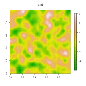
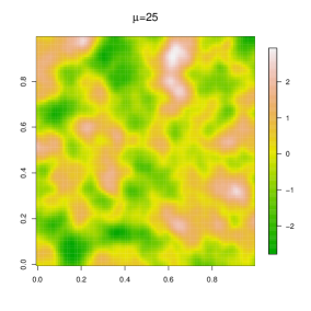
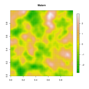
Fig. 2: Four realizations of a Gaussian RF with $\varphi_{\nu,\mu,\beta}$ correlation model when $\nu=2$, $\beta=0.0338$ and $\mu=5,10,25$ and the limit case when $\mu\to\infty$, that is the Matérn model ${\cal M}_{\nu+1/2,\beta}$ (on the bottom right corner).

Figure 2 shows four realizations of a zero-mean Gaussian RF with ${\cal GW}_{\nu,\mu,\delta_{\nu,\mu,\beta}}$ correlation model using the same parameter settings of Figure 1. For the four realizations we use a common Gaussian simulation using Cholesky decomposition. It can be appreciated that the realizations are very smooth (the sample paths are $2$ times differentiable in this case), and they look very similar, even if the first three realizations come from Gaussian RFs with compactly supported correlation functions.

Finally, we point out that the Matérn model is attained as limit when the smoothness parameter is greater than or equal than $0.5$. This implies that the full range of validity of the smoothness parameter is not covered. In particular, the proposed model is not able to parameterize the fractal dimension [21] of the associated Gaussian RF as in the Matérn case.

4 Numerical experiments

4.1 Speed of convergence

In the absence of theoretical rates of convergence, we show some simple numerical results on the convergence of the $\varphi_{\nu,\mu,\beta}$ to the Matérn model when increasing $\mu$. Specifically, we analyze the absolute error

$$E_{\mu,\nu}(r):=|\varphi_{\nu,\mu,\beta}(r)-{\cal M}_{\nu+1/2,\beta}(r)|,\quad r\geq 0,$$ (24)

when increasing $\mu$ given $\nu$ and $\beta$.

In particular in Figure 3 (first row) we plot $\varphi_{\nu,\mu,\beta}$ , for $\mu=\lambda(2,\nu),5,10,20,40,60,80$ and ${\cal M}_{\nu+1/2,\beta}$ for $\nu=0,1,2$. Here the $\beta$ parameter is chosen such that the practical range of the Matérn model model is approximately equal to $0.5$ ($\beta=0.167,0.105,0.084$, respectively, for $\nu=0,1,2$). The second row displays the associated values of $E_{\mu,\nu}$. It can be appreciated that $E_{\mu,\nu}$ decreases when increasing $\mu$ for each $\nu$, as expected from Theorem 3 and the magnitude of the absolute error is increasing with $\nu$. In addition, the third row depicts the spectral densities associated to the correlation models in the first row. Note that the approximation is getting better for the high-frequency components as $\mu$ increases and it deteriorates when increasing $\nu$. These simple numerical examples shows that the speed of convergence depends on the smoothness parameter $\nu$. Table 2 more deeply depicts the convergence of the proposed model to Matérn by reporting the maximum absolute error under a more general parameter setting. Table 2 confirms that $\varphi_{\nu,\mu,\beta}$ approaches ${\cal M}_{\nu+1/2,\beta}$ when increasing $\mu$ and the maximum absolute error between them strongly depends on $\nu$.

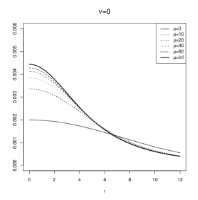
Fig. 3: First row: the $\varphi_{\nu,\mu,\beta}(r)$ model with $\mu=\lambda(2,\nu),5,10,20,40,80$ and $\mu\to\infty$ (the Matérn model) and with $\beta=0.167,0.105,0.084$ and $\nu=0,1,2$ (from left to right) respectively. Second row: associated absolute value error $E_{\mu,\nu}(r)$ as defined in (24). Third row: spectral densities associated with the correlation models in the first row.

Table 2: Maximum of $E_{\mu,\nu}$ as defined in (24) when increasing $\mu$ for $\nu=0,0.5,\ldots,2.5$.

$\mu$	$\lambda(d,\nu)$	5	$10$	$20$	$40$	$80$	$160$	$320$	$640$
$\nu=0.0$	$0.22944$	0.05799	$0.02800$	$0.01376$	$0.00682$	$0.00340$	$0.00170$	$0.00085$	$0.00042$
$\nu=0.5$	$0.25586$	$0.11010$	$0.05643$	$0.02857$	$0.01438$	$0.00721$	$0.00361$	$0.00181$	$0.00090$
$\nu=1.0$	$0.27001$	0.15470	$0.08346$	$0.04345$	$0.02218$	$0.01121$	$0.00564$	$0.00283$	$0.00141$
$\nu=1.5$	$0.27914$	$0.19257$	$0.10856$	$0.05800$	$0.03004$	$0.01529$	$0.00772$	$0.00388$	$0.00194$
$\nu=2.0$	$0.28554$	$0.22475$	$0.13164$	$0.07205$	$0.03782$	$0.01940$	$0.00983$	$0.00494$	$0.00248$
$\nu=2.5$	$0.29029$	$0.25230$	$0.15279$	$0.08552$	$0.04549$	$0.02350$	$0.01195$	$0.00603$	$0.00303$

4.2 On the asymptotic distribution of the maximum likelihood estimator

This Section focus on the ML estimation of the proposed covariance model. Let $D$ be a subset of ${\rm I\!R}^{d}$ and $S_{n}=\{\bm{s}_{1},\ldots,\bm{s}_{n}\in D\}$ denote any set of distinct locations. Let $\bm{Z}_{n}=(Z(\bm{s}_{1}),\ldots,Z(\bm{s}_{n}))^{\top}$ be a finite realization of a zero-mean stationary Gaussian RF $Z=\{Z(\bm{s}),\bm{s}\in D\}$, with isotropic covariance function $\sigma^{2}\varphi_{\nu,\mu,\beta}$. Here, $\top$ denotes transposition.

We then write $R_{n}(\bm{\tau})=[\varphi_{\bm{\tau}}(\|\bm{s}_{i}-\bm{s}_{j}\|)]_{i,j=1}^{n}$ with $\bm{\tau}=(\nu,\mu,\beta)^{\top}$ for the associated correlation matrix. If $\bm{\theta}=(\sigma^{2},\bm{\tau})^{\top}$, the Gaussian log-likelihood function is defined as follows:

$$\mathcal{L}_{n}(\bm{\theta})=-\frac{1}{2}\left(n\log(2\pi\sigma^{2})+\log(|R_{n}(\bm{\tau})|)+\frac{1}{\sigma^{2}}\bm{Z}_{n}^{\top}R_{n}(\bm{\tau})^{-1}\bm{Z}_{n}\right),$$ (25)

and $\widehat{\bm{\theta}}_{n}:=\text{argmax}_{\bm{\theta}\in\bm{\theta}}\mathcal{L}_{n}(\bm{\theta})$ is the ML estimator of $\bm{\theta}$. [33] provide general conditions for the consistency and the asymptotic normality of the ML estimator irrespective of the correlation model. Under suitable conditions, $\widehat{\bm{\theta}}_{n}$ is consistent and asymptotically normal, that is $\widehat{\bm{\theta}}_{n}-\bm{\theta}\stackrel{{\scriptstyle\mathcal{D}}}{{\longrightarrow}}\mathcal{N}\left(\bm{0},F^{-1}_{n}(\bm{\theta})\right)$ as $n\to\infty$ where

$$\bm{F}_{n}(\bm{\theta})=\left[\frac{1}{2}\textrm{tr}\left(\Sigma_{n}(\bm{\theta})^{-1}\frac{d\Sigma_{n}(\bm{\theta})}{d\bm{\theta}_{i}}\Sigma_{n}(\bm{\theta})^{-1}\frac{d\Sigma_{n}(\bm{\theta})}{d\bm{\theta}_{j}}\right)\right]_{i,j=1}^{p}.$$ (26)

is the Fisher Information matrix and $\Sigma_{n}(\bm{\theta})=\sigma^{2}R_{n}(\bm{\tau})$. The conditions are normally difficult to verify and they assume indirectly that the sample set grows in such a way that the sampling domain increases in extent as $n$ increases (i.e., $||\bm{s}_{i}-\bm{s}_{j}||\geq c>0$), which implies that the set $D$ is unbounded.

Under fixed domain asymptotics, no general results are available for the asymptotic properties of ML estimator. For the Generalized Wendland model they have been studied in [6]. In particular, using Theorem 4 in [6], it can be shown that if $P(\sigma_{i}^{2}\varphi_{\nu,\mu_{i},\beta_{i}})$, $i=0,1$, are two zero mean Gaussian measures and if $\mu_{i}>\nu+d+0.5$ then for any bounded infinite set $D\subset{\rm I\!R}^{d}$, $d=1,2,3$, $P(\sigma^{2}_{0}\varphi_{\nu,\mu_{0},\beta_{0}})\equiv P(\sigma^{2}_{1}\varphi_{\nu,\mu_{1}\beta_{1}})$ on the paths of $Z$ if and only if

$$\frac{\sigma_{0}^{2}}{\beta^{2\nu+1}_{0}}g(\nu,\mu_{0})=\frac{\sigma_{1}^{2}}{\beta^{2\nu+1}_{1}}g(\nu,\mu_{1}).$$ (27)

where $g(\nu,\mu)={\Gamma(\mu+1)}/{\Gamma(2\nu+\mu+1)}$. A straight consequence is that for fixed $\nu$, the $\beta$, $\mu$ and $\sigma^{2}$ parameters cannot be estimated consistently under fixed domain asymptotics. Instead, the microergodic parameter

$$c(\bm{\theta})=\frac{\sigma^{2}}{\beta^{1+2\kappa}}g(\nu,\mu)$$

is consistently estimable. Additionally, using Theorem 8 in [6], for any fixed $\nu$ and $\mu\geq\lambda(d,\nu)+3$ as $n\to\infty$, the asymptotic distribution of ML estimator of the microergodic parameter is given by

$$\sqrt{n}\left(\frac{\hat{\sigma}_{n}^{2}}{\hat{\beta}_{n}^{2\nu+1}}g(\nu,\mu)-c(\bm{\theta})\right)\stackrel{{\scriptstyle\mathcal{D}}}{{\longrightarrow}}N\left(0,2c(\bm{\theta})^{2}\right).$$

where $\hat{\beta}_{n}$ and $\hat{\sigma}_{n}^{2}$ are ML estimators of $\beta$ and $\sigma^{2}$.

We analyze the performance of the ML method when estimating the parameters of the covariance model $\sigma^{2}\varphi_{\nu,\mu,\beta}$ from both increasing and fixed domain asymptotics perspective. In particular we focus on assessing the approximation given by the asymptotic distribution of the ML estimation under both types of asymptotics.

We first simulate $500$ realizations of a zero mean Gaussian RF with covariance model $\sigma^{2}\varphi_{\nu,\mu,\beta}$ observed over $n=1000$ location sites uniformly distributed in the unit square. The smoothness parameter is assumed to be known and fixed equal to $\nu=0,1,2$. We set $\sigma^{2}=1$, $\mu=\lambda(2,\nu)+x$ with $x=1,2,4$ and since the increasing as well as the fixed-domain frameworks can be mimicked by fixing the number of location sites over a given spatial domain and decreasing or increasing the spatial dependence [55, 30], we set the $\beta$ parameter, such that the compact support $\delta_{\nu,\mu,\beta}$ is identically equal to $0.15$ and $0.6$ for each scenario. For instance, when $\nu=0$ and $\mu=\lambda(2,0)+2=3.5$ then $\beta=0.15/3.5$ to obtain a compact support equal to $\delta_{0,3.5,\beta}=0.15$.

In the ML estimation of $(\sigma^{2},\beta,\mu)^{\top}$ for the covariance model $\sigma^{2}\varphi_{\nu,\mu,\beta}$, we found a reparameterization of the $\mu$ parameter to be useful by considering its inverse. That is, we consider the ML estimation of $(\sigma^{2},\beta,\mu^{*})^{\top}$ where $\mu^{*}=1/\mu\in[0,1/\lambda(2,\nu)]$ for the covariance model $\sigma^{2}\varphi_{\nu,1/\mu^{*},\beta}$. In the original parameterization, we found high variability in the ML estimates of the $\mu$ parameter, particularly for large values of $\mu$. A similar pattern has been observed in literature when estimating the degrees of freedom of the Student’s $t$ distribution; to alleviate this issue some authors [13, 2] propose to considering the estimation of the inverse degrees of freedom.

Figure 4 reports the boxplots of the centered and rescaled ML estimates $(\widehat{\mu_{i}^{*}}-\mu^{*})/\sqrt{f_{11}}$, $(\widehat{\beta}_{i}-\beta)/\sqrt{f_{22}}$, $(\widehat{\sigma^{2}_{i}}-\sigma^{2})/\sqrt{f_{33}}$, $i=1,\ldots,500$ (first, second and third rows, respectively), when $\nu=0,1,2$ (first, second and third column respectively), $\mu=\lambda(2,\nu)+x$ with $x=1,2,4$ ( for each subfigure ) by considering increasing and fixed domain asymptotics scenarios $\delta=0.15,0.6$ (left and right part of each subfigure respectively). Here $f_{ii}$ are the diagonal elements of the inverse of the Fisher information matrix in Equation (26). Using the asymptotic results under increasing domain asymptotics the displayed boxplots should be similar to the boxplot of a Gaussian random variable. Overall the asymptotic distribution seems to work reasonably well (at least for values between the first and third quartiles) and, as expected, the asymptotic approximation worsens when switching from the increasing domain ($\delta=0.15$) to the fixed domain ($\delta=0.60$) setting, irrespective of the values of $\mu$ and $\nu$.

	$\nu=0$		$\nu=1$		$\nu=2$
	$\delta=0.15$	$\delta=0.6$	$\delta=0.15$	$\delta=0.6$	$\delta=0.15$	$\delta=0.6$
$\widehat{\mu^{*}}$
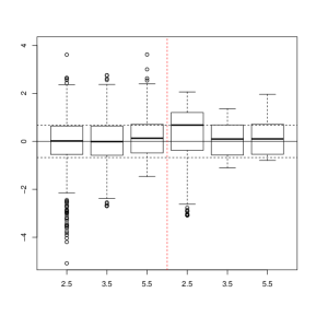
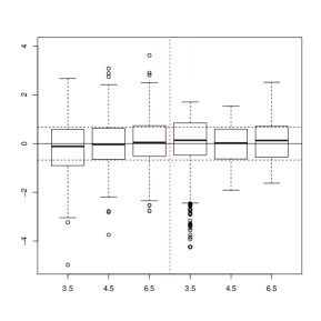
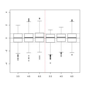
$\widehat{\beta}$
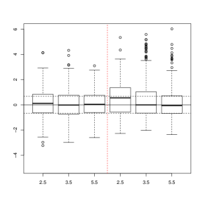
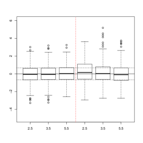
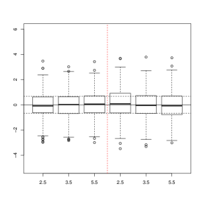
$\widehat{\sigma}^{2}$
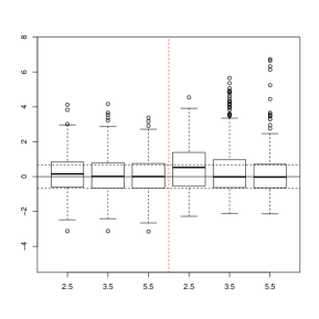
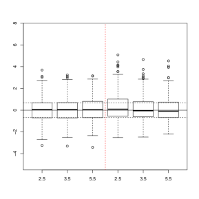
$m(\widehat{\sigma}_{i}^{2},\widehat{\beta}_{i})$

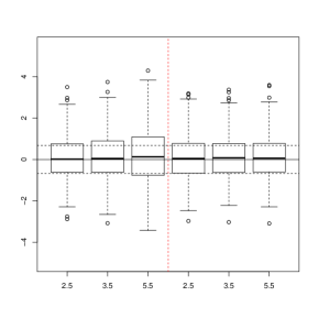
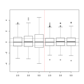
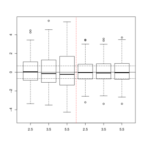
Fig. 4: Boxplots of the centered and rescaled ML estimates $(\widehat{\mu_{i}^{*}}-\mu^{*})/\sqrt{f_{11}}$, $(\widehat{\beta}_{i}-\beta)/\sqrt{f_{22}}$, $(\widehat{\sigma^{2}_{i}}-\sigma^{2})/\sqrt{f_{33}}$, $i=1,\ldots,500$ of the covariance model $\sigma^{2}\varphi_{\nu,1/\mu^{*},\beta}$ with $\mu^{*}=1/\mu$ when $\nu=0,1,2$, $\mu=\lambda(2,\nu)+x$, $x=1,2,4$ and $\beta$ is such that the compact support $\delta_{\nu,\mu,\beta}=0.15,0.6$ (left and right part of each subfigure). Last row: boxplots of $m(\widehat{\sigma}_{i}^{2},\widehat{\beta}_{i})=\sqrt{n/2}(\widehat{\sigma^{2}}_{i}(\widehat{\beta}_{i},\mu)\widehat{\beta}_{i}^{-(1+2\kappa)}/\sigma^{2}\beta^{-(1+2\kappa)}-1)$, $i=1,\ldots,500$. The horizontal dotted lines represent the quantiles of the order $0.25$ and $0.75$ of the standard Gaussian distribution.

To analyze the approximation given by the asymptotic distribution under fixed domain of the microergodic parameter $\sigma^{2}\beta^{-(1+2\kappa)}g(\nu,\mu)$, we replicate the previous numerical experiment using the same simulation settings but this time, we assume that $\mu$ is known and fixed. Last row of Figure 4 depicts the boxplots of $m(\widehat{\sigma}_{i}^{2},\widehat{\beta}_{i})=\sqrt{n/2}(\widehat{\sigma}_{i}^{2}\widehat{\beta}_{i}^{-(1+2\kappa)}/\sigma^{2}\beta^{-(1+2\kappa)}-1)$, $i=1,\ldots,500$, for each $\nu$ and $\mu$. Also in this case the boxplots should be similar to the boxplot of a standard Gaussian random variable. As expected, the asymptotic approximation works much better under fixed domain asymptotics ($\delta=0.60$), and it seems to improve with decreasing $\nu$. In addition, under increasing domain the approximation clearly deteriorates when increasing both $\mu$ and $\nu$.

5 Data Examples

We consider two data examples that explain, from our perspective, how the proposed model should be used depending on the size of the available dataset. The first approach involves the estimation of the $\mu$ parameter and should be applied to (not necessarily) small spatial datasets with the goal of looking for an improvement of the Matérn family from modeling viewpoint. The second approach is more suitable for large datasets and considers an arbitrary fixed $\mu$. In this case the goal is to seek highly sparse matrices to reduce the computational complexity.

5.1 Application to Mean Temperature Data

We consider data from WorldClim (www.worldclim.org) a global database of high spatial resolution global weather and climate data for the years 1970-2000 [15]. In particular, we consider mean temperature data of September over a specific region of French (see Figure 5 (a)) observed at $624$ geo-referenced location sites. Following [31], we first detrend the data using splines to remove the cyclic pattern of both variables along the longitude and latitude directions, and then regard the residuals $y(\bm{s}_{i})$, $i=1,\ldots,n$, $n=624$ as a realization from a zero mean Gaussian RF with isotropic covariance function $\sigma^{2}\rho(r)$ (the empirical semi-variogram is depicted in Figure 5 (b)). For the isotropic correlation function $\rho(r)$ we specify the proposed reparametrized Generalized Wendland correlation model. In particular, we consider $\varphi_{\nu,\mu,\beta}$ for $\nu=0,1$ and the associated special limit case, that is the Matérn model ${\cal M}_{\nu+1/2,\beta}$ for $\nu=0,1$.

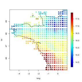
(a)	(b)

Fig. 5: From left to right: a) spatial locations of mean temperature of September in a specific region of France and b) empirical semivariogram of the residuals after detrending the original data.

Here, we adopt an increasing domain approach by estimating all parameters of the covariance models with ML method, and we compute the associated standard error estimation, as the square root of diagonal elements of the inverse of the Fisher Information matrix (26). For the $\mu$ parameter we use the parameterization described in Section 4.2 that is, $\mu^{*}=1/\mu\in(0,\lambda(2,\nu)^{-1}]$ and the Matérn model, under this parametrization, is attained when $\mu^{*}\to 0$.

The results of the estimation are summarized in Table 3, where we also report the values of the maximized log-likelihoods and the associated values of Akaike information criterion (AIC). It can be appreciated that the covariance model $\sigma^{2}\varphi_{0,\mu^{*},\beta}$ achieves the lower AIC with respect to the Matérn model $\sigma^{2}{\cal M}_{0.5,\beta}$. When $\nu=1$, the reparametrized Generalized Wendland model $\sigma^{2}\varphi_{1,\mu^{*},\beta}$ coincides with the Matérn model ${\cal M}_{1.5,\beta}$ since the estimation of the $\mu^{*}$ parameter collapses to the lower bound. For this reason in Table 3 we only report the estimates of the covariance model $\sigma^{2}{\cal M}_{1.5,\beta}$. Overall the best fitted covariance model is $\sigma^{2}\varphi_{0,\mu^{*},\beta}$. Figure 6 provides a graphical comparison between the empirical and estimated semivariograms using the $\sigma^{2}{\cal M}_{0.5,\beta}$ and $\sigma^{2}\varphi_{0,\mu^{*},\beta}$ covariance models, respectively.

Fig. 6: Empirical semivariogram versus estimated semivariogram using the Matérn model $\sigma^{2}{\cal M}_{0.5,\beta}$ (left part) and the Generalized Wendland model $\sigma^{2}\varphi_{0,\mu^{*},\beta}$ (right part) covariance models.

Table 3: ML estimates with associated standard error (in parentheses), RMSE, LSCORE and CRPS for the three Gaussian RFs with underlying covariance functions $\sigma^{2}\varphi_{0,\mu^{*},\beta}$, its special limit case $\sigma^{2}{\cal M}_{0.5,\beta}$ and $\sigma^{2}{\cal M}_{1.5,\beta}$.

	$\beta$	$\sigma^{2}$	$\mu^{*}$	-loglik	AIC	RMSE	LSCORE	CRPS
$\sigma^{2}{\cal M}_{0.5,\beta}$	$160.0165$ $(79.263)$	$0.1222$ $(0.059)$		$464.25$	$-924.5$	$0.0932$	$0.1965$	$0.0923$
$\sigma^{2}{\cal\varphi}_{0,\mu^{*},\beta}$	$103.7678$ $(7.239)$	$0.0787$ $(0.008)$	$0.6342$ $(0.047)$	$470.86$	$-935.7$	$0.0926$	$0.1950$	$0.0916$
$\sigma^{2}{\cal M}_{1.5,\beta}$	$16.3599$ $(0.899)$	$0.06163$ $(0.008)$		$457.65$	$-911.3$	$0.0947$	$0.2627$	$0.0928$

We further evaluate the predictive performances of the three Gaussian RFs. We use the following resampling approach: we randomly choose 80% of the spatial locations and we use the remaining 20% as data for the predictions. We then use the estimates in Table 3 to compute three prediction scores [20] for each Gaussian RF. Specifically, for each $j-th$ left-out sample $(y_{j}^{L}(\bm{s}_{1}),\ldots,y_{j}^{L}(\bm{s}_{K}))$, for $j=1,\ldots,1000$ we compute

1. the root mean squared error

   $$\overline{\mathrm{RMSE}}_{j}=\left[\frac{1}{K}\sum_{i=1}^{K}\left(y_{j}^{L}(\bm{s}_{i})-\widehat{Y}_{j}^{L}(\bm{s}_{i})\right)^{2}\right]^{\frac{1}{2}}$$

2. the logarithmic score

   $$\overline{\log S}_{j}=\frac{1}{K}\sum_{i=1}^{K}\left[\frac{1}{2}\log\{2\pi\sigma^{L}_{j}(\bm{s}_{i})\}+\frac{1}{2}\{z^{L}_{j}(\bm{s}_{i})\}^{2}\right],$$ (28)

3. the continuous ranked probability

   $$\overline{{\rm CPRS}}_{j}=\frac{1}{K}\sum_{i=1}^{K}\sigma_{j}(\bm{s}_{i})\left(z^{L}_{j}(\bm{s}_{i})\left(2\Phi(z^{L}_{j}(\bm{s}_{i}))-1\right)+2\Phi(z^{L}_{j}(\bm{s}_{i}))-\frac{1}{\sqrt{\pi}}\right),$$ (29)

where $\widehat{Y}_{j}^{L}(\bm{s}_{i})$ is the optimal linear predictor, $\sigma^{L}_{j}(\bm{s}_{i})$ is the corresponding square root variance and $z^{L}_{j}(\bm{s}_{i})=(y^{L}_{j}(\bm{s}_{i})-\widehat{Y}_{j}^{L}(\bm{s}_{i}))/\sigma^{L}_{j}(\bm{s}_{i})$. Table 3 reports the overall means $\mathrm{RMSE}=\sum_{j=1}^{1000}\overline{\mathrm{RMSE}}_{j}/1000$, $\mathrm{\log S}=\sum_{j=1}^{1000}\overline{\log S}_{j}/1000$ and $\mathrm{CRPS}=\sum_{j=1}^{1000}\overline{{\rm CPRS}}_{j}/1000$ for each of the eight Gaussian RFs. As expected, the covariance model $\sigma^{2}\varphi_{0,\mu^{*},\beta}$ outperforms the Matérn model limit case ${\cal M}_{0.5,\beta}$ and the Matérn model ${\cal M}_{1.5,\beta}$ for the three prediction scores considered.

5.2 Application to Yearly total precipitation anomalies

We consider the dataset in Kaufman et al. [29] of yearly total precipitation anomalies $\bm{z}=\{z(\bm{s}_{i})$, $i=1,\ldots,n$} registered at $n=7,352$ location sites in the USA since 1895 to 1997. The yearly totals have been standardized by the long-run mean and standard deviation for each station from 1962 (Figure 7, right part). Kaufman et al. [29] adapted a zero-mean Gaussian random field with an exponential covariance model using covariance tapering to reduce the computational costs associated with ML estimation and optimal linear prediction. Here we present an improved analysis by considering a zero mean Gaussian RF with correlation:

$$\rho^{*}(r)=(1-\tau^{2})\rho(r)+\tau^{2}I(r=0),\quad.r\geq 0,$$ (30)

that includes a nugget effect $0\leq\tau^{2}<1$, as suggested by inspecting the empirical semivariogram in Figure 7, with a correlation function $\rho(r)$ specified as ${\cal M}_{0.5,\beta}$ and its generalization $\varphi_{0,\mu,\beta}$. For the $\varphi_{0,\mu,\beta}$ model, to obtain sparse covariance matrices we fixed different values of $\mu=1.5,1.75,2,2.5,3.5,4.5$ and let $\bm{\theta}=(\tau^{2},\sigma^{2},\beta)^{\top}$ to be estimated for each of the six Gaussian RFs.

The bottleneck when maximizing the likelihood function or computing the optimal liner predictor is the Cholesky decomposition which generally has $O(n^{3})$ time and $O(n^{2})$ memory complexity. If the matrix is sparse, then the computation of the Cholesky factor can be hastened by using sparse matrix algorithms and the computational performance of the factorization depends on the percentage of zero elements of the covariance matrix and on how the locations are ordered.

We point out that ML estimation can partially take advantage of the computational benefits associated with the proposed model: for a fixed smoothness parameter, the compact support depends on $\beta$ and $\mu$. Even when considering a fixed $\mu$, the covariance matrix can be highly or slightly sparse, depending on the value of $\beta$ in the optimization process. An alternative strategy is to use estimation methods with a good balance between statistical efficiency and computational complexity that do not require any restrictions on the covariance model, such as composite likelihood methods [14, 7] or multi-resolution approximation methods [27] or more in general using Vecchia’s approximations [28]. However, in this application we consider ML estimation which is still computational feasible although very slow to obtain.

Table 4 depicts the ML estimates of $\bm{\theta}$ with associated standard error for ${\cal M}_{0.5,\beta}$ and $\varphi_{0,\mu,\beta}$, $\mu=1.5,1.75,2,2.5,3.5,4.5$ along with the associated maximized log-likelihood. It can be appreciated that the maximized log-likelihood increases with increasing $\mu$, and that the Matérn performs the best fitting in this case. For each model, Table 4 also reports the percentage of zero entries in the estimated covariance matrix $\Sigma(\hat{\bm{\theta}})$ and the estimated compact support $\widehat{\delta}_{0,\mu,\hat{\beta}}=\mu\hat{\beta}$. As expected, the percentage decreases and $\widehat{\delta}_{0,\mu,\hat{\beta}}$ increases with increasing $\mu$.

Clear computational gains can be achieved using the proposed model when computing the optimal linear kriging predictor which requires the computation of the Cholesky factor of $\Sigma(\hat{\bm{\theta}})$. To provide an idea of the computational gains, Table 4 reports, the time needed for the computation of the Cholesky factor of $\Sigma(\hat{\bm{\theta}})$ using the R package spam [17] when using $\hat{\sigma}^{2}{\cal M}_{0.5,\hat{\beta}}$ and $\hat{\sigma}^{2}\varphi_{0,\mu,\hat{\beta}}$ for $\mu=1.5,1.75,2,2.5,3.5,4.5$. The time in seconds is expressed in terms of elapsed time, using the function system.time of the R software on a laptop with a 2.4 GHz processor and 16 GB of memory.

It is apparent that the computational saving with respect to the Matérn model can be huge when decreasing $\mu$. In particular when $\mu=1.5$ the computation of the Cholesky factor is approximately 50 times faster with respect the Matérn case. However, the loss of prediction efficiency is generally very small. To compare the models in terms of prediction performance, we have used leave-one-out cross-validation as described in Zhang and Wang [54]. In particular the authors show that RMSE, LSCORE and CRPS leave-one-out cross-validation can be computed in just one step by using the estimated covariance matrix. In Table 4 we report RMSE, LSCORE and CRPS for the correlation models considered and the three prediction scores for the Matérn model and its generalization are quite similar when $\mu\geq 2$. In this specific example, taking into account the balance between computational complexity, statistical efficiency and prediction performance, a good choice for the correlation model could be $\varphi_{0,2,\beta}$.

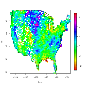
(a)	(b)

Fig. 7: From left to right: a) coloured map of precipitation anomalies data. b) empirical semivariogram of precipitation anomalies data.

Table 4: ML estimates for the parameters of the Matérn model ${\cal M}_{0.5,\beta}$ and the proposed model $\varphi_{0,x,\beta}$ for $x=1.5,1.75,2.5,3.5,4.5$. Prediction measures RMSE, LSCORE, and CRPS based on leave-one-out cross-validation are also reported. The estimated compact support $\hat{\delta}_{0,\mu,\hat{\beta}}=\mu\hat{\beta}$, the percentage of zeros in the estimated covariance matrix and the computational time (in seconds) to perform the associated Cholesky decomposition are also reported.

	$\hat{\tau}^{2}$	$\hat{\beta}$	$\hat{\sigma}^{2}$	-loglik	RMSE	LSCORE	CRPS	$\widehat{\delta}_{0,\mu,\hat{\beta}}=\mu\hat{\beta}$	$\%$	TIME
$\varphi_{0,1.5,\beta}$	$0.1002$ $(0.008)$	$266.38$ $(2.20)$	$1.112$ $(0.047)$	$-5443.78$	$0.4691$	$0.9647$	$0.6444$	$399.57$	$0.939$	$1.86$
$\varphi_{0,1.75,\beta}$	$0.0945$ $(0.008)$	$298.88$ $(7.48)$	$1.179$ $(0.053)$	$-5405.82$	$0.4674$	$0.9607$	$0.6410$	$523.04$	$0.905$	$2.78$
$\varphi_{0,2,\beta}$	$0.0964$ $(0.007)$	$295.21$ $(5.29)$	$1.1547$ $(0.053)$	$-5393.02$	$0.4668$	$0.9595$	$0.6396$	$590.42$	$0.884$	$3.63$
$\varphi_{0,2.5,\beta}$	$0.1103$ $(0.008)$	$247.48$ $(8.16)$	$0.999$ $(0.048)$	$-5391.58$	$0.4669$	$0.9594$	$0.6396$	$618.70$	$0.874$	$4.07$
$\varphi_{0,3.5,\beta}$	$0.1110$ $(0.011)$	$243.75$ $(23.86)$	$0.9905$ $(0.085)$	$-5388.47$	$0.4669$	$0.9594$	$0.6396$	$853.13$	$0.791$	$9.17$
$\varphi_{0,4.5,\beta}$	$0.1195$ $(0.013)$	$216.45$ $(27.49)$	$0.9078$ $(0.092)$	$-5386.23$	$0.4669$	$0.9593$	$0.6393$	$974.03$	$0.743$	$11.9$
${\cal M}_{0.5,\beta}$	$0.1334$ $(0.012)$	$167.24$ $(18.58)$	$0.7729$ $(0.062)$	$-5377.68$	$0.4668$	$0.9585$	$0.6383$	$\infty$	0	$95.25$

6 Conclusions

This paper shows that the celebrated Matérn covariance model is actually a special limit case of a more general compactly supported covariance model which is a reparameterized version of the generalized Wendland family. As a consequence, the (reparametrized) Generalized Wendland model is more flexible than the Matérn model with an extra-parameter that allows for switching from compactly to globally supported covariance functions.

On the one hand the proposed family can be potentially more efficient with respect to the Matérn family when modeling the covariance function of point-referenced spatial data, as shown, for instance in the first real data application. On the other hand, depending on the size of the available dataset, the proposed model can potentially lead to (highly) sparse correlation matrices by fixing the extra-parameter $\mu$, with clear computational savings with respect to the Matérn model as shown in the second real data application. Further details on computational gains when handling sparse matrices with sparse matrices algorithms can be found in [16], [29], [17], [9] and [36] just to mention a few.

Most of the literature on modeling spatial or spatiotemporal multivariate data modeling is based on the Matérn model as a building block (see [44], [35] and [19], to name a few). Thus, our results open new doors and opportunities in spatial statistics. For instance, [32] developed an approximation of Gaussian RFs with the Matérn covariance model using a Gaussian Markov RF. The connection is established through a specific stochastic partial differential equation (SPDE), formulation in that a Gaussian RF with Matérn covariance is a solution to the SPDE. It could be of theoretical interest to find a generalization of this specific SPDE exploiting, for instance, the results given in [10]. However, the spectral density of the proposed model cannot be written as the reciprocal of a polynomial. As a consequence the associated Gaussian RF is Markovian only when $\mu\to\infty$.

For some important special cases the proposed covariance model can be easily calculated, as in the Matérn case (see Table 1). More generally, the proposed model can be easily implemented since efficient numerical computation of the Gaussian hypergeometric function can be found in different libraries such as the GNU scientific library [22] and the most important statistical softwares including R, MATLAB and Python. In particular, the R package GeoModels [8] used in this paper for the numerical experiments and the application computes the proposed model using the Python implementation of the Gaussian hypergeometric function in the SciPy library [46].

References

References

- Abramowitz and Stegun [1970] M. Abramowitz, I. A. Stegun (Eds.), Handbook of Mathematical Functions, Dover, New York, 1970.
- Arellano-Valle and Azzalini [2013] R. B. Arellano-Valle, A. Azzalini, The centred parameterization and related quantities of the skew-t distribution, Journal of Multivariate Analysis 113 (2013) 73 – 90. Special Issue on Multivariate Distribution Theory in Memory of Samuel Kotz.
- Askey [1973] R. Askey, Radial characteristic functions, Technical report, Research Center, University of Wisconsin (1973).
- Banerjee et al. [2004] S. Banerjee, B. P. Carlin, A. E. Gelfand, Hierarchical Modeling and Analysis for Spatial Data, Chapman & Hall/CRC Press, Boca Raton: FL, 2004.
- Banerjee and Gelfand [2003] S. Banerjee, A. Gelfand, On smoothness properties of spatial processes, Journal of Multivariate Analysis 84 (2003) 85 – 100.
- Bevilacqua et al. [2019a] M. Bevilacqua, T. Faouzi, R. Furrer, E. Porcu, Estimation and prediction using Generalized Wendland functions under fixed domain asymptotics, The Annals of Statistics 47 (2019a) 828–856.
- Bevilacqua and Gaetan [2014] M. Bevilacqua, C. Gaetan, Comparing composite likelihood methods based on pairs for spatial Gaussian random fields, Statistics and Computing (2014) 1–16.
- Bevilacqua et al. [2019b] M. Bevilacqua, V. Morales-Oñate, C. Caamaño-Carrillo, Geomodels: A package for geostatistical Gaussian and non Gaussian data analysis, https://vmoprojs.github.io/GeoModels-page/, 2019b. R package version 1.0.3-4.
- Bevilacqua et al. [2016] M. Bevilacqua, A. F. R., C.Gaetan, E. Porcu, D. Velandia, Covariance tapering for multivariate gaussian random fields estimation, Statistical Methods and Application 25(1) (2016) 21–556.
- Carrizo-Vergara et al. [2018] R. Carrizo-Vergara, D. Allard, N. Desassis, A general framework for spde-based stationary random fields, arXiv preprint arXiv:1806.04999 (2018).
- Chernih et al. [2014] A. Chernih, S. I.H., R. Womersley, Wendland functions with increasing smoothness converge to a Gaussian, Adv. Comput. Math. 40 (2014) 185–200.
- Cressie and Wikle [2011] N. Cressie, C. Wikle, Statistics for Spatio-Temporal Data., Wiley Series in Probability and Statistics. Wiley, 2011.
- DiCiccio and Monti [2011] T. J. DiCiccio, A. C. Monti, Inferential aspects of the skew tdistribution, Quaderni di Statistica 13 (2011) 1–21.
- Eidsvik et al. [2014] J. Eidsvik, B. A. Shaby, B. J. Reich, M. Wheeler, J. Niemi, Estimation and prediction in spatial models with block composite likelihoods, Journal of Computational and Graphical Statistics 23 (2014) 295–315.
- Fick and Hijmans [2017] S. Fick, R. Hijmans, Worldclim 2: new 1km spatial resolution climate surfaces for global land areas, International Journal of Climatology 37 (2017) 4302–4315.
- Furrer et al. [2006] R. Furrer, M. G. Genton, D. Nychka, Covariance tapering for interpolation of large spatial datasets, Journal of Computational and Graphical Statistics 15 (2006) 502–523.
- Furrer and Sain [2010] R. Furrer, S. R. Sain, spam: a sparse matrix R package with emphasis on MCMC methods for Gaussian Markov random fields, Journal of Statistical Software 36 (2010) 1–25.
- Gneiting [2002] T. Gneiting, Compactly supported correlation functions, Journal of Multivariate Analysis 83 (2002) 493–508.
- Gneiting et al. [2010] T. Gneiting, W. Kleiber, M. Schlather, Matérn Cross-Covariance functions for multivariate random fields, Journal of the American Statistical Association 105 (2010) 1167–1177.
- Gneiting and Raftery [2007] T. Gneiting, A. E. Raftery, Strictly proper scoring rules, prediction, and estimation, Journal of the American Statistical Association 102 (2007) 359–378.
- Gneiting et al. [2012] T. Gneiting, H. Sevcikova, D. B. Percival, Estimators of fractal dimension: Assessing the roughness of time series and spatial data, Statistical Science 27 (2012) 247–277.
- Gough [2009] B. Gough, GNU scientific library reference manual, Network Theory Ltd., 2009.
- Gradshteyn and Ryzhik [2007] I. Gradshteyn, I. Ryzhik, Table of Integrals, Series, and Products, Academic Press, New York, 7 edition, 2007.
- Guttorp and Gneiting [2006] P. Guttorp, T. Gneiting, Studies in the history of probability and statistics xlix on the Matèrn correlation family, Biometrika 93 (2006) 989–995.
- Heaton et al. [2019] M. J. Heaton, A. Datta, A. O. Finley, R. Furrer, J. Guinness, R. Guhaniyogi, F. Gerber, R. B. Gramacy, D. Hammerling, M. Katzfuss, F. Lindgren, D. W. Nychka, F. Sun, A. Zammit-Mangion, A case study competition among methods for analyzing large spatial data, Journal of Agricultural, Biological, and Environmental Statistics 24 (2019) 398–425.
- Hubbert [2012] S. Hubbert, Closed form representations for a class of compactly supported radial basis functions, Adv. Comput. Math. 36 (2012) 115–136.
- Katzfuss [2017] M. Katzfuss, A multi-resolution approximation for massive spatial datasets, Journal of the American Statistical Association 112 (2017) 201–214.
- Katzfuss and Guinness [2021] M. Katzfuss, J. Guinness, A general framework for vecchia approximations of gaussian processes, Statist. Sci. 36 (2021) 124–141.
- Kaufman et al. [2008] C. G. Kaufman, M. J. Schervish, D. W. Nychka, Covariance tapering for likelihood-based estimation in large spatial data sets, Journal of the American Statistical Association 103 (2008) 1545–1555.
- Kaufman and Shaby [2013] C. G. Kaufman, B. A. Shaby, The role of the range parameter for estimation and prediction in geostatistics, Biometrika 100 (2013) 473–484.
- Li and Zhang [2011] B. Li, H. Zhang, An approach to modeling asymmetric multivariate spatial covariance structures, Journal of Multivariate Analysis 102 (2011) 1445–1453.
- Lindgren et al. [2011] F. Lindgren, H. Rue, J. Lindström, An explicit link between Gaussian fields and Gaussian Markov random fields: the stochastic partial differential equation approach, Journal of the Royal Statistical Society: Series B 73 (2011) 423–498.
- Mardia and Marshall [1984] K. V. Mardia, J. Marshall, Maximum likelihood estimation of models for residual covariance in spatial regression, Biometrika 71 (1984) 135–146.
- Matèrn [1986] B. Matèrn, Spatial Variation: Stochastic Models and their Applications to Some Problems in Forest Surveys and Other Sampling Investigations, Springer, Heidelberg, 2nd edition, 1986.
- Paciorek and Schervish [2006] C. J. Paciorek, M. J. Schervish, Spatial modelling using a new class of nonstationary covariance functions, Environmetrics 17 (2006) 483–506.
- Porcu et al. [2020] E. Porcu, M. Bevilacqua, M. Genton, Nonseparable, space-time covariance functions with dynamical compact supports, Statistica Sinica 30 (2020) 719–739.
- Prudnikov et al. [1986] A. P. Prudnikov, Y. A. Brychkov, O. I. Marichev, Integrals and Series: More Special Functions, volume 3, Gordon and Breach Science Publishers, New York, 1986.
- Schaback [2011] R. Schaback, The missing Wendland functions, Advances in Computational Mathematics 34 (2011) 67–81.
- Schoenberg [1938] I. J. Schoenberg, Metric spaces and completely monotone functions, Annals of Mathematics 39 (1938) 811–841.
- Shaby and Ruppert [2012] B. Shaby, D. Ruppert, Tapered covariance: Bayesian estimation and asymptotics, Journal of Computational and Graphical Statistics 21 (2012) 433–452.
- Stein [1988] M. Stein, Asymptotically efficient prediction of a random field with a misspecified covariance function, The Annals of Statistics 16 (1988) 55–63.
- Stein [1990] M. L. Stein, Uniform asymptotic optimality of linear predictions of a random field using an incorrect second order structure, The Annals of Statistics 19 (1990) 850–872.
- Stein [1999] M. L. Stein, Interpolation of Spatial Data. Some Theory of Kriging, Springer, New York, 1999.
- Stein [2005] M. L. Stein, Space-time covariance functions, Journal of the American Statistical Association 100 (2005) 310–321.
- Stein [2013] M. L. Stein, Statistical properties of covariance tapers, Journal of Computational and Graphical Statistics 22 (2013) 866–885.
- Virtanen et al. [2020] P. Virtanen, R. Gommers, T. Oliphant, M. Haberland, T. Reddy, D. Cournapeau, E. Burovski, P. Peterson, W. Weckesser, B. Jonathan, van der Walt, S. J., M. Brett, J. Wilson, K. Jarrod Millman, N. Mayorov, et al., SciPy 1.0: Fundamental Algorithms for Scientific Computing in Python, Nature Methods 17 (2020) 261–272.
- Wang and Loh [2011] D. Wang, W.-L. Loh, On fixed-domain asymptotics and covariance tapering in Gaussian random field models, Electronic Journal of Statistics 5 (2011) 238–269.
- Wendland [1995] H. Wendland, Piecewise polynomial, positive definite and compactly supported radial functions of minimal degree, Advances in Computational Mathematics 4 (1995) 389–396.
- Whittle [1954] P. Whittle, On stationary processes in the plane, Biometrika (1954) 434–449.
- Yaglom [1987] A. M. Yaglom, Correlation Theory of Stationary and Related Random Functions. Volume I: Basic Results, Springer, New York, 1987.
- Zastavnyi and Trigub [2002] V. Zastavnyi, R. Trigub, Positive definite splines of special form, English transl. in Sb. Math. 193 (2002) 1771–1800.
- Zastavnyi [2000] V. P. Zastavnyi, On positive definiteness of some functions, Journal of Multivariate Analysis 73 (2000) 55–81.
- Zhang [2004] H. Zhang, Inconsistent estimation and asymptotically equivalent interpolations in model-based geostatistics., Journal of the American Statistical Association 99 (2004) 250–261.
- Zhang and Wang [2010] H. Zhang, Y. Wang, Kriging and cross-validation for massive spatial data, Environmetrics 21 (2010) 290–304.
- Zhang and Zimmerman [2005] H. Zhang, D. Zimmerman, Towards reconciling two asymptotic frameworks in spatial statistics, Biometrika 92 (2005) 921–936.