Binomial ideals of domino tilings

Abstract.

In this paper, we consider the set of all domino tilings of a cubiculated region. The primary question we explore is: How can we move from one tiling to another? Tiling spaces can be viewed as spaces of subgraphs of a fixed graph with a fixed degree sequence. Moves to connect such spaces have been explored in algebraic statsitics. Thus, we approach this question from an applied algebra viewpoint, making new connections between domino tilings, algebraic statistics, and toric algebra. Using results from toric ideals of graphs, we are able to describe moves that connect the tiling space of a given cubiculated region of any dimension. This is done by studying binomials that arise from two distinct domino tilings of the same region. Additionally, we introduce tiling ideals and flip ideals and use these ideals to restate what it means for a tiling space to be flip connected. Finally, we show that if $R$ is a $2$-dimensional simply connected cubiculated region, any binomial arising from two distinct tilings of $R$ can be written in terms of quadratic binomials. As a corollary to our main result, we obtain an alternative proof to the fact that the set of domino tilings of a $2$-dimensional simply connected region is connected by flips.

1. Introduction and Background

A $2\times 1$ domino (or a $1\times 2$ domino) is two unit squares joined along a single edge. A domino tiling of a region is a covering of the region with dominos such that there are no gaps or overlaps. As an area of mathematical research, domino tilings appeared as early as 1937 in the context of thermodynamics and dimer systems [9]. Several bodies of work in the 2-dimensional setting show that such objects are rich and nuanced [13] [8], [25], [7], [4], [14], [18]. For example, Kasteleyn and Fisher–Temperley proved independently [8, 13] that the number of tilings of a $2n\times 2m$ rectangle is

$$4^{mn}\prod_{j=1}^{m}\prod_{k=1}^{n}\Big{(}\cos^{2}\frac{2\pi}{2m+1}+\cos^{2}\frac{k\pi}{2n+1}\Big{)}.$$

While, there is no closed-form expression for the number of domino tilings of an arbitrary $2$-dimensional region, there are many papers that study this problem for specific types of regions, such as Aztec diamonds and pyramids [1, 19, 23]. Higher dimensional regions, such as $3$-dimensional regions, have also been explored. For example, in 1998, Ciucu gave an upper bound on the number of $3$-dimensional domino tilings of a $n\times n\times n$ cube [3].

In lieu of a complete enumeration of the tilings of a region, one can estimate the number of tilings through Monte Carlo Markov chain sampling methods. Such methods require a set of moves that connect the space, which lead us to our primary question of interest: What are sets of moves that connect the space of domino tilings for a fixed region? We tackle this question from an algebra lens, making a new connection between domino tilings, algebraic statistics, and combinatorial commutative algebra through toric ideals of graphs.

For $2$-dimensions, it is known that any two domino tilings of a simply connected region can be obtained through a sequence of flips [25, 22]. Generalizing results to higher dimensions has been of interest to fields from combinatorics to solid state chemistry [7, 18]. However, previous results, such as those built on Thurston’s height function [20] fail to generalize to the $3$-dimensional setting. In fact, in $3$-dimensions even the most uncomplicated of regions fail to be flip connected. For instance the domino tilings of $l\times m\times n$ box are not connected by flips [10, 13, 15]. Milet and Saldanha introduced another local move called the trit, which operates on three dominoes at a time (as opposed to the flip that operates on two dominoes at a time) [15]. While some $3$-dimensional tiling spaces are connected by flips and trits, not all are; [15] includes some examples. In [10], Klivans et al. give conditions in terms of topological invariants for testing whether two different $3$-dimensional domino tilings are connected by flips or by flips and trits.

Our paper explores the connectivity question by noting that the space of tilings of a region $R$ corresponds to a particular fiber of a design matrix $A$, where $A$ is prescribed by the region $R$ (here we are using language from algebraic statistics, which is defined formally in the Section 3). By appealing to algebraic statistics, and in particular, the Fundamental Theorem of Algebraic Statistics [6], for any given region, of any dimension, we can find a set of moves that is guaranteed to connect its tiling space by finding a set of generators of the toric ideal of A, a binomial ideal. Using the well-known correspondence between domino tilings of a region $R$ and perfect matchings of an associated graph $G_{R}$ [27] and results in combinatorial commutative algebra on toric ideals of graphs [16], in Theorem 3.8, we describe the moves guaranteed to connect the tiling space in terms of the graph $G_{R}$. The moves described in Theorem 3.8 are not always local flips though. While we can show that if the toric ideal of $G_{R}$ is quadratic, then the space of tilings of $R$ is flip connected, the converse is not always true. In order to explore flip connected tiling spaces more, we introduce two additional binomial ideals, the tiling ideal and the flip ideal. These ideals are not always prime, and thus not always toric, however we can describe exactly when a tiling space is flip connected using these two ideals (Theorem 3.12). Finally, we showcase this algebraic perspective by providing an alternative proof to the fact that the tiling space of any simply connected region of $\mathbb{R}^{2}$ is flip connected.

This paper is organized as follows. In Section 2, we formally define domino tilings and discuss tilings from a graph theoretic viewpoint. In Section 3, we discuss the connection of tiling spaces to algebraic statistics and toric ideals of graphs and describe a set of moves guaranteed to connect the tiling space of a given region. Additionally, we introduce the tiling ideal and the flip ideal of a region $R$ and restate what it means for a tiling space to be connected in terms of these two ideals. Finally, in Section 4, we show, using algebraic techniques, that the tiling space of any simply connected region of $\mathbb{R}^{2}$ is flip connected.

2. Domino Tilings

Let $R$ be a $n$-dimensional cubiculated region of $\mathbb{R}^{N}$, i.e. a homogeneous cubical complex of dimension $n$ embedded in $\mathbb{R}^{N}$ with $n\leq N$. A $d$-dimensional domino is two adjacent elementary $n$-dimensional cubes connected along a face of dimension $n-1$; we will denote the set of dominos contained in $R$ as $\mathcal{D}_{R}$. A domino tiling $T\subseteq\mathcal{D}_{R}$ of a cubiculated region $R$ is defined to be a covering of $R$ with dominoes such that every elementary cube of $R$ is covered exactly once; we will denote the space of all tilings of $R$ as $\mathcal{T}_{R}$. We are interested in local moves that connect all the tilings in $\mathcal{T}_{R}$. A move between two tilings $T_{1},T_{2}\in\mathcal{T}_{R}$ is an ordered pair $M=(D_{1},D_{2})$ of two sets of dominoes $D_{1},D_{2}\subseteq\mathcal{D}_{R}$ such that $T_{2}=(T_{1}\setminus D_{1})\cup D_{2}$. For simplicity, if $M$ is a move from $T_{1}$ to $T_{2}$, we will write $T_{2}=T_{1}+M$. We say a move has size $d$ if $|D_{1}|=|D_{2}|=d$. We begin our discussion with the simplest move, the local flip, or flip.

Definition 2.1.

A local flip is performed by replacing a pair of two adjacent parallel dominoes, i.e. two dominoes that share two $n-1$ dimensional faces, with two adjacent parallel dominoes in a perpendicular direction to the first pair. We will refer to the set of all flip moves for $R$ as $\mathcal{M}_{R_{flip}}$.

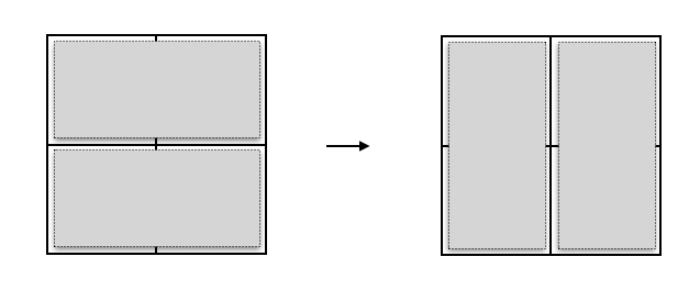
Figure 1. A local flip.

Definition 2.2.

Let $R$ be a cubiculated region, and let $\mathcal{M}_{R}$ be a set of possible moves of $R$. We say $\mathcal{M}_{R}$ connects $\mathcal{T}_{R}$ if for every two tilings $T_{1},T_{2}\in\mathcal{T}_{R}$, there exists $M_{1},\ldots M_{r}\in\mathcal{M}_{R}$ such that $T_{2}=T_{1}+M_{1}+M_{2}+\ldots M_{r}$ and $T_{1}+M_{1}+\ldots M_{s}\in\mathcal{T}_{R}$ for all $1\leq s\leq r$.

Two tilings $T_{1}$ and $T_{2}$ are flip connected if there exists a sequence $M_{1},\ldots,M_{r}\in\mathcal{M}_{R_{flip}}$ such that $T_{2}=T_{1}+M_{1}+\ldots M_{r}$ and $T_{1}+M_{1}+\ldots M_{s}\in\mathcal{T}_{R}$ for all $1\leq s\leq r$. A cubiculated region $R$ is flip connected if every two tilings of $R$ are flip connected. It is known that if a $2$-dimensional region is simply connected then its corresponding space of tilings is flip connected.

Theorem 2.3.

[25, 22] If $R$ is a simply connected region in $2$-dimensions, then $\mathcal{T}_{R}$ is flip connected.

In [25], and more explicitly in [22], Theorem 2.3 is proved via the construction and analysis of a map from the vertices of a domino tiling to $\mathbb{Z}$ called the height function. In this paper, we give an alternative proof of the theorem using binomial ideals.

2.1. Connections to graph theory

In order to apply tools from combinatorial commutative algebra, it is helpful to think of tilings of a cubiculated region as perfect matchings of a graph. Here we set up the terminology to construct this correspondence.

Let $R$ be a $n$-dimensional cubiculated region. Let $G_{R}$ be the undirected simple graph that has one vertex for each elementary cube in $R$ and an edge between a pair of vertices if their two corresponding cubes in $R$ share a $n-1$ dimensional face. Given a graph $G=(V,E)$, a matching $M$ is an independent edge set. A perfect matching is a matching that covers all vertices in $G$. By the construction of $G_{R}$ from $R$, we see that there is a one-to-one correspondence between tilings of $R$ and perfect matchings on the graph $G_{R}$. This correspondence is illustrated in Figure 2.

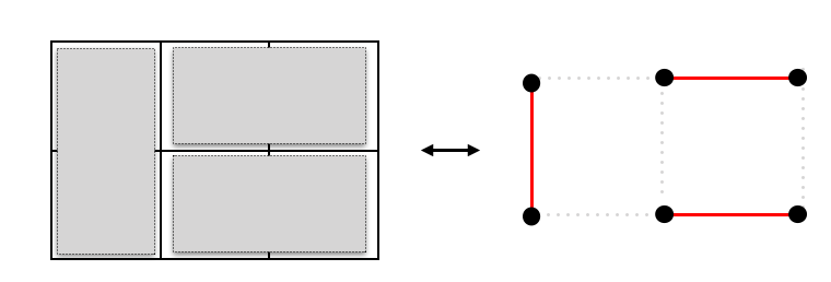
Figure 2. Let $R=B_{2,3}$, the $2\times 3$ box. On the left is a tiling on $R$, on the right is a perfect matching of $G_{2,3}$.

Example 2.4.

Let the region $R$ be the $m\times\ell$ box denoted $B_{m,\ell}$. Then $G_{R}$ is denoted by $G_{m,\ell}$ and is the $m\times\ell$ grid graph whose vertices correspond to the points in $[0,m]\times[0,\ell]\cap\mathbb{Z}^{2}$.

Remark 2.5.

Since $R$ can always be viewed as a subregion of a $n$-dimensional box $B_{m_{1},\ldots,m_{n}}$, the graph $G_{R}$ is a subgraph of the grid graph $G_{m_{1},\ldots,m_{n}}$.

For the rest of this paper, we will refer to tilings and matchings interchangeably. We will use the underlying graph structure to understand the connectivity of the space of $2$-dimensional domino tilings for a region $R$. While tilings on a cubiculated region $R$ can be characterized by perfect matchings on $G_{R}$, moves between two tilings can be characterized by even cycles.

Definition 2.6.

A walk on $G$ is a finite sequence of the form

$$w=\big{(}(v_{1},v_{2}),(v_{2},v_{3}),\dots,(v_{n-1},v_{n})\big{)}$$

with each $v_{i}\in V(G)$ and $\{v_{i-1},v_{i}\}\in E(G)$. In the case where $v_{1}=v_{n}$, then $w$ is called a closed walk. A cycle is a closed walk that traverses each vertex in the walk exactly once. The length of a cycle or closed walk is the number of edges in the walk. A closed walk is even if the cycle has even length. An even closed walk is primitive if it does not contain a proper closed even subwalk.

Proposition 2.7.

Let $R$ be a cubiculated region. Every cycle of the graph $G_{R}$ is even.

Proof.

As implied by Remark 2.5, for any cubiculated region $R$, the graph $G_{R}$ is a subgraph of a grid graph $G_{m_{1},\ldots,m_{n}}$. In particular, $G_{R}$ is bipartite. Thus, every cycle of $G_{R}$ is even [27]. ∎

Remark 2.8.

Since every cycle of $G_{R}$ is even, the only primitive even closed walks on $G_{R}$ are cycles [16].

In the following proposition, we see that the union of two tilings of $R$ corresponds to a collection of cycles on $G_{R}$.

Proposition 2.9.

Let $T_{1}$ and $T_{2}$ be tilings and let $G=T_{1}\cup T_{2}$ (considered as a multigraph). Then $G$ will be a disjoint collection of even cycles, some of which may be $2$-cycles.

Proof.

Consider the graph $G=T_{1}\cup T_{2}$ with $n$ vertices. We know for each $i\in V(G)$ the $deg_{G}(i)=2$. By definition $G$ must be a $2$-regular graph of size $n$. A characterization of $2$-regular graphs gives us that $G$ will be formed by a disjoint collection of cycles. ∎

Since $G=T_{1}\cup T_{2}$ is a disjoint collection of cycles we introduce the following terminology.

Definition 2.10.

Let $G$ be a graph. We say $\mathcal{C}=\{\mathcal{C}_{1},\mathcal{C}_{2},\ldots,\mathcal{C}_{r}\}$ is a cycle cover of $G$ if each $\mathcal{C}_{i}$ is a cycle and every vertex in $G$ is covered by exactly one $\mathcal{C}_{i}$.

Note that given a region $R$ and two tilings, $T_{1}$ and $T_{2}$, the multigraph $\mathcal{C}=T_{1}\cup T_{2}$ is a cycle cover of $G_{R}$. Additionally, we can think of the edges in $\mathcal{C}$ as two-colorable, specifically, we can color the edges corresponding to $T_{1}$ red and the edges corresponding to $T_{2}$ as blue. This coloring will be helpful in later sections.

Finally, we end this section with a discussion on chords, which will play a role in the algebra in the next two sections.

Definition 2.11.

Let $\mathcal{C}$ be a cycle of a graph $G=(V,E)$. An edge $e\in E$ is a chord of $\mathcal{C}$ if $e$ connects two vertices covered by $\mathcal{C}$, but is not in $\mathcal{C}$. A cycle is chordless if it does not have a chord in $G$.

Definition 2.12.

Let $\mathcal{C}=\big{(}(v_{1},v_{2}),(v_{2},v_{3}),\dots,(v_{n-1},v_{n})\big{)}$ be an even cycle of a graph $G=(V,E)$. We say $e=\{v_{i},v_{j}\}\in E(G)$ is a chord of $\mathcal{C}$ with $i<j$. Furthermore, we call $e$ an even chord if $j-i$ is odd, in other words, if the two new cycles obtained by adding $e$ to $\mathcal{C}$ are both even.

3. Tilings and Toric Ideals of Graphs

In this section, we introduce toric ideals of graphs and their connections to tiling spaces. Toric ideals of graphs have been well-studied (see, for example, [26, 16, 17, 21, 24, 12, 11]). By making the connection to toric ideals of graphs, we can describe a set of moves that is guaranteed to connect the tiling space $\mathcal{T}_{R}$ for any cubiculated region $R$.

3.1. Toric ideals of graphs and Markov bases

Let $G=(V,E)$ be a graph. Consider the following two polynomial rings

$$\mathbb{K}[E] =\mathbb{K}[y_{e}\mid e\in E[G]],\text{ and}$$

$$\mathbb{K}[V] =\mathbb{K}[x_{v}\mid v\in V(G)].$$

Let $\phi_{G}$ be the ring homomorphism defined as follows

$$\phi_{G}:\mathbb{K}[E] \to\mathbb{K}[V]$$

$$y_{(i,j)} \mapsto x_{i}x_{j}.$$

The toric ideal of $G$, denoted $I_{G}$, is defined to be the kernel of the map $\phi_{G}$

$$I_{G}:=\ker(\phi_{G})=\{f\in\mathbb{K}[E]\ :\ \phi_{G}(f)=0\}.$$

For our application, we are going to be most interested in the generating set of a toric ideal of a graph. Such generating sets can be described by primitive closed even walks. Furthermore, when $G$ is bipartite, a generating set of $I_{G}$ can be given simply in terms of even cycles.

Definition 3.1.

Let $w$ be an even cycle, i.e.

$$w=\Big{(}(v_{1},v_{2}),(v_{2},v_{3}),\dots,(v_{2n},v_{1})\Big{)}$$

where $e_{i}=\{v_{i},v_{i+1}\}$. The binomial arising from $w$ is

$$B_{w}=\prod_{i=1}^{n}y_{e_{2i-1}}-\prod_{i=1}^{n}y_{e_{2i}}.$$

Proposition 3.2.

Given a bipartite graph $G$, the ideal $I_{G}$ is generated by the set of binomials arising from even cycles on $G$ [26].

Just as we can define a binomial arising from a cycle, we can define a binomial associated to two tilings. Regard two tilings $T_{1}$ and $T_{2}$ of a cubiculated region $R$ as perfect matchings in $G_{R}$.

Definition 3.3.

Define the binomial arising from $(T_{1},T_{2})$ to be

$$B_{T_{1},T_{2}}=\prod_{e_{i}\in T_{1}}y_{e_{i}}-\prod_{e_{j}\in T_{2}}y_{e_{j}}.$$

Note that if $R$ is a cubiculated region and $T_{1},T_{2}\in\mathcal{T}_{R}$, then the binomial $B_{T_{1},T_{2}}$ arising from $(T_{1},T_{2})$ is in the toric ideal $I_{G_{R}}$ since

$$\phi_{G_{R}}(B_{T_{1},T_{2}})=\prod_{e_{i}\in T_{1}}\phi_{G_{R}}\big{(}y_{e_{i}}\big{)}-\prod_{e_{j}\in T_{2}}\phi_{G_{R}}\big{(}y_{e_{j}}\big{)}=\prod_{i\in V(G_{R})}x_{i}-\prod_{i\in V(G_{R})}x_{i}=0.$$

Remark 3.4.

For ease of notation, we will use the following monomial shorthand. Let $E_{0}\subseteq E(G)$, then we define

$$y^{E_{0}}:=\prod_{e_{i}\in E_{0}}y_{e_{i}}.$$

Thus, we will write $B_{T_{1},T_{2}}$ as

$$B_{T_{1},T_{2}}=y^{T_{1}}-y^{T_{2}}.$$

Similar to a binomial $B_{T_{1},T_{2}}$ arising from two tilings, the binomial arising from a tiling move $(D_{1},D_{2})$ is $B_{D_{1},D_{2}}=y^{D_{1}}-y^{D_{2}}$ and is also in $I_{G_{R}}$.

We can describe a way to move between any two tilings in $\mathcal{T}_{R}$ by invoking the Fundamental Theorem of Markov Bases from algebraic statistics [5, 6]. To do this we now build a connection between toric ideals of graphs and the language of Markov bases. First, let’s describe $I_{G}$ in an alternate way using design matrices. Indeed, the most common way to define a toric ideal is through an integer matrix $A$; this matrix is referred to as the design matrix in algebraic statistics. Let $A$ be the vertex-edge incidence matrix of $G$ with $N=\#E(G)$ columns. Then

$$I_{G}=I_{A}:=\langle y^{u}-y^{v}\ |\ u,v\in\mathbb{Z}_{\geq 0}^{N},Au=Av\rangle.$$

In this setting, we can think about $u,v\in\mathbb{Z}_{\geq 0}^{N}$ as integer vectors or as multisets of edges drawn from $E(G)$. The condition $Au=Av$ means that $u$ and $v$ have the same degree sequence as multigraphs.

Let $u\in\mathbb{Z}_{\geq 0}^{N}$. The fiber of $u$ with respect to $A$ is

$$\mathcal{F}(u)=\{v\in Z_{\geq 0}^{N}:Av=Au\}.$$

The fiber of $u$ is precisely the collection of all multigraphs with edges drawn from $E(G)$ with same degree sequence as $u$. Since every tiling of $R$ has the same degree sequence when viewed as a perfect matching of $G_{R}$, it is the case that $\mathcal{T}_{R}=\mathcal{F}(T)$ for any tiling $T$ of $R$. This key observation allows us to use Markov bases to find a set of moves to connect $\mathcal{T}_{R}$.

Definition 3.5.

Let $A\in\mathbb{Z}^{M\times N}$. Let $\text{ker}_{\mathbb{Z}}A=\{v\in\mathbb{Z}^{N}:Av=0\}$ be the integer kernel of $A$. A finite set $\mathcal{MB}\subset\text{ker}_{\mathbb{Z}}A$ is called a Markov basis for $A$ if for all $u\in\mathbb{Z}_{\geq 0}^{N}$ and $v\in\mathcal{F}(u)$, there is a sequence $b_{1},\ldots,b_{r}\in\pm\mathcal{MB}:=\{(-1)^{i}b\ :\ b\in\mathcal{MB},\ i=0,1\}$ such that

$$v=u+\sum_{k=1}^{r}b_{k}\text{ and }u+\sum_{k=1}^{s}b_{k}\geq 0\text{ for all }s=1,\ldots r.$$

The elements of a Markov basis are called Markov moves.

When $A$ is the vertex-edge incidence matrix of $G_{R}$ for a cubiculated region $R$, every Markov move $b$ with $0,1$, and $-1$ entries corresponds to a move $M=(D_{1},D_{2})$ on $R$ by letting $D_{1}$ be the set of edges whose corresponding entries of $b$ have value $-1$ and $D_{2}$ be the set of edges whose corresponding entries of $b$ have value $1$. Let $b_{D_{1},D_{2}}$ be the vector in $\{-1,0,1\}^{N}$ that corresponds to the move $(D_{1},D_{2})$. If $\mathcal{MB}$ is a Markov basis for $A$, then $\mathcal{MB}_{sf}:=\mathcal{MB}\cap\{-1,0,1\}^{N}$ connects $\mathcal{T}_{R}$ (due to the fact that every tiling in $\mathcal{T}_{R}$ can be viewed as a $0-1$ vector and thus applying a move not in $\{-1,0,1\}^{N}$ would move us outside of the fiber $\mathcal{T}_{R}$).

The Fundamental Theorem of Markov Bases gives a way to test whether or not a set $\mathcal{MB}$ is indeed a Markov basis.

Theorem 3.6.

[5] Let $\mathcal{MB}=\{b_{1},\dots,b_{n}\}\subset\mathbb{Z}^{N}$ be a set of vectors; note that every vector $b_{i}$ can be written uniquely as the difference $b_{i}=b_{i}^{+}-b_{i}^{-}$ of two non-negative vectors with disjoint support. The set $\mathcal{MB}=\{b_{1},\dots,b_{n}\}$ is a Markov basis for the matrix $A$ if and only if the corresponding set of binomials $\{x^{b_{i}^{+}}-x^{b_{i}^{-}}\}_{i=1,\dots,n}$ generates the toric ideal $I_{A}$ .

Recall that a move is size $d$ if $|D_{1}|=|D_{2}|=d$.

Theorem 3.7.

If $I_{G_{R}}$ is generated by binomials of degree $d$ or less, then the set of tilings of a cubiculated region $R$ is connected by moves of size $d$ or less.

Proof.

Let $A$ be the vertex-edge incidence matrix of $G_{R}$. Assume $I_{G_{R}}$ is generated by binomials of degree $d$ or less. Then by Theorem 3.6, this means that there is a Markov basis $\mathcal{MB}$ for $A$ whose moves all have size $d$ or less. Since a Markov basis connects every fiber of $A$, and $\mathcal{T}_{R}$ is a fiber of $A$, the set $\mathcal{MB}$ connects $\mathcal{T}_{R}$. ∎

Theorem 3.8.

(Moves that connect tilings spaces) Let $R$ be a cubiculated region with the associated graph $G_{R}$. Let $\mathcal{M}_{cycles}$ be the set of moves on $\mathcal{T}_{R}$ corresponding to the set of chordless cycles of $G_{R}$, i.e.

$$\mathcal{M}_{cycles}:=\{b_{D_{1},D_{2}}\ :\ D_{1}\cup D_{2}\text{ is a chordless cycle of }G_{R}\}.$$

Then $\mathcal{M}_{cycles}$ connects $\mathcal{T}_{R}$.

Proof.

By Lemma 3.1 and 3.2 in [16], since $I_{G_{R}}$ is bipartite, $I_{G_{R}}$ is generated by binomials arising from chordless cycles of $G_{R}$. This means, by Theorem 3.6, $\mathcal{M}_{cycles}$ is a Markov basis for the vertex-edge incidence matrix of $G_{R}$, thus, $\mathcal{M}_{cycles}\subset\{-1,0,1\}^{N}$ connects $\mathcal{T}_{R}$. ∎

Corollary 3.9.

Let $2d$ be the size of the largest chordless cycle in $G_{R}$. Then the space of tilings of $R$ is connected by moves of size $d$ or less.

Note that Corollary 3.9 holds for any $R$ in any dimension. However, in many instances, especially in the 2-dimensional setting, the bound given in Corollary 3.9 is far from sharp. This is due to the fact that tiling binomials can usually be written without using the larger degree generators of $I_{G}$, as we will see in Section 4.

Example 3.10.

  

(a) The graph $G_{R}$ of the cubiculated region $R$ in row (a) of Figure 3 has a single chordless cycle of length $10$. This means $I_{G_{R}}$ is a principal ideal generated by a binomial of degree $5$. The region $R$ has exactly two tilings that are connected by the tiling move of size $5$ that corresponds to the generating binomial of $I_{G_{R}}$.

(b) The largest cycle of the graph $G_{R}$ of the cubiculated region $R$ in row (b) of Figure 3 is length $8$. However, this length $8$ cycle is not chordless. In fact, $G_{R}$ has no chordless cycles of length $>4$. This means $I_{G_{R}}$ is generated by quadratics and $\mathcal{T}_{R}$ is flip connected. Indeed, by this same reasoning and applying Theorem 3.8, we can conclude if $R$ is the $2\times\ell$ box $B_{2,\ell}$, then $\mathcal{T}_{R}$ is flip connected.

(c) The graph $G_{R}$ of the cubiculated region $R$ in row (c) of Figure 3 has a chordless cycle of length $10$. The degree $5$ binomial in $I_{G}$ corresponding to this cycle is an indispensable binomial of $I_{G}$ [21], meaning that there exists a nonzero constant multiple of it in every minimal system of binomial generators of $I_{G}$. However, unlike the region in row (a), for this region, the space of tilings $\mathcal{T}_{R}$ is flip connected and we do not need the size $5$ move to connect the space of tilings.

(d) The graph $G_{R}$ of the cubiculated region R in row (d) of Figure 3 has a chordless cycle of length $6$, which corresponds to the trit move described in [15]. The cubic binomial in $I_{G}$ corresponding to this cycle is an indispensable binomial of $I_{G}$. However, for this region, the space of tilings $\mathcal{T}_{R}$ is flip connected and we do not need the trit move; in fact, for $R$, there is no tiling for which we can apply the trit move.

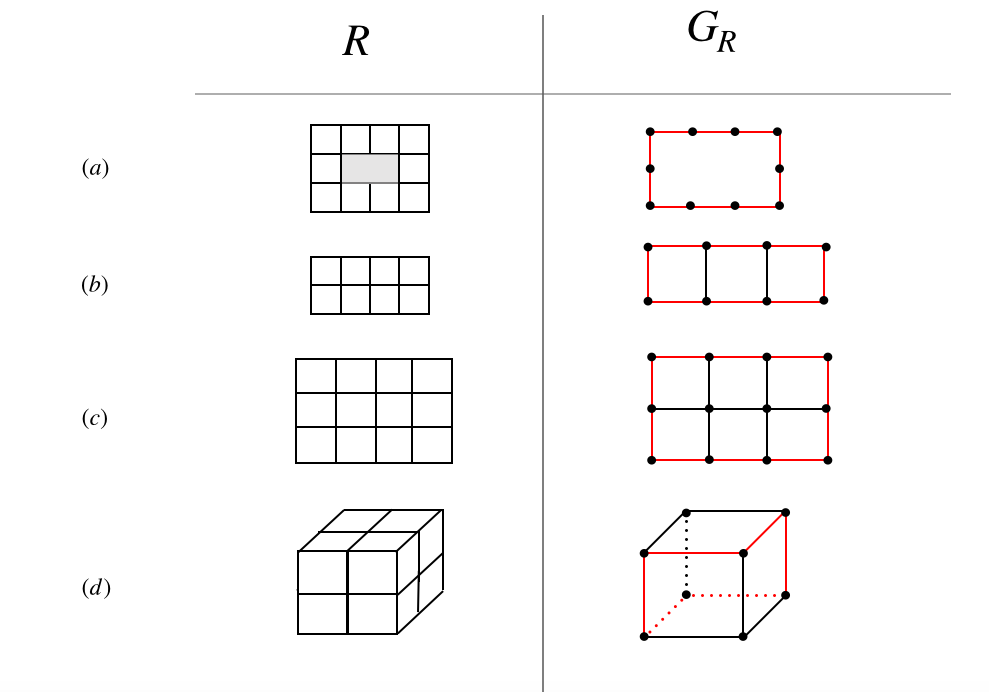
Figure 3. Four cubiculated regions and their corresponding graphs with the largest cycle highlighted.

3.2. Tiling and flip ideals

Theorem 3.8 and Corollary 3.9 give a bound on the size of moves needed to connect the space of tilings of a region $R$, however, this bound can be arbitrarily large. For example, let $m,n\geq 3$, then $G_{m,n}$ contains a chordless cycle of length $2(m+n)$.

A local flip $(D_{1},D_{2})$ corresponds to a $4$-cycle in $G_{R}$ and the corresponding binomial $y^{D_{1}}-y^{D_{2}}$ has degree $2$. Conversely, any non-zero quadratic binomial in $I_{G_{R}}$ must correspond to a $4$-cycle, and consequently, a flip move. Thus, to show $\mathcal{T}_{R}$ is flip connected, we need to show that every binomial arising from two tilings is generated by quadratics.

Definition 3.11.

Let $R$ be a cubiculated region with associated graph $G_{R}$. The flip ideal of $R$ is defined as follows:

$$I_{R_{flip}}:=\langle y^{D_{1}}-y^{D_{2}}\ :\ (D_{1},D_{2})\in\mathcal{M}_{flip}\rangle\subseteq I_{G_{R}}.$$

The tiling ideal of $R$ is defined as follows:

$$I_{R_{tiling}}:=\langle y^{T_{1}}-y^{T_{2}}\ :T_{1},\ T_{2}\in\mathcal{T}_{R}\ \rangle\subseteq I_{G_{R}}.$$

Using the flip and tiling ideal, we can use the language of ideals to restate what it means for a region to be flip connected.

Theorem 3.12.

A tiling space $\mathcal{T}_{r}$ of a cubiculated region $R$ is flip connected if and only if

$$I_{R_{tiling}}\subseteq I_{R_{flip}}.$$

For a region $R$, both the flip ideal and the tiling ideal ideal are subideals of the toric ideal of the graph $G_{R}$:

$$I_{R_{tiling}}\subseteq I_{G_{R}}\ \ \ \ \ \ \ \ \ \ \ \ \ \ \ \ I_{R_{flip}}\subseteq I_{G_{R}}.$$

When $G_{R}$ contains no chordless cycles of length $>4$, we have $I_{R_{flip}}=I_{G_{R}}$, and thus, $I_{R_{tiling}}\subseteq I_{flip}$ and $R$ is flip connected.

While $I_{R_{tiling}}$ and $I_{R_{flip}}$ are binomial ideals, unlike $I_{G_{R}}$ they are not always prime ideals and therefore not always toric ideals. However, the primary decomposition of the flip ideal of a region has interesting combinatorics. Indeed, working from an earlier version of this manuscript, in [2], Chin explores the flip ideals of $3\times\ell$ box regions and gives a complete description of their primary decompositions.

We now explore the three ideals $I_{G_{R}}$, $I_{R_{tiling}}$, and $I_{R_{flip}}$ and their possible relationships through four examples.

Example 3.13.

Let $R=B_{2,3}$, the $2\times 3$ box.

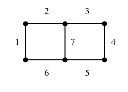
Figure 4. The graph $G_{2,3}$ with edges labeled.

Using the labeling in Figure 4, we have

1. $I_{G_{R}}=\langle\;y_{1}y_{7}-y_{2}y_{6},\;y_{4}y_{7}-y_{3}y_{5}\;\rangle$,
   

2. $I_{R_{tiling}}=\langle\;y_{1}y_{3}y_{5}-y_{2}y_{4}y_{6},\;y_{1}y_{4}y_{7}-y_{1}y_{3}y_{5},\;y_{1}y_{4}y_{7}-y_{2}y_{4}y_{6}\;\rangle$,
   

3. $I_{R_{flip}}=\langle\;y_{4}y_{7}-y_{3}y_{5},\;y_{1}y_{7}-y_{2}y_{6}\;\rangle$.
   

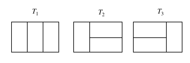
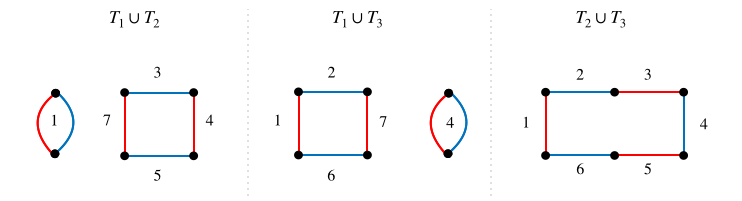
Figure 5. On top are the three tilings, $T_{1},T_{2}$, and $T_{3}$, of the $2\times 3$ box. On bottom are the three cycle covers of $G_{2,3}$ formed by the possible pairs of tilings.

The three tilings of $R$ are depicted in Figure 5. Notice that the last binomial listed in the generating set of $I_{R_{tiling}}$ is not needed and we could have written $I_{R_{tiling}}=\langle y_{1}y_{3}y_{5}-y_{2}y_{4}y_{6},y_{1}y_{4}y_{7}-y_{1}y_{3}y_{5}\rangle$. For this region, it is the case that

$$I_{R_{tiling}}\subseteq I_{R_{flip}}=I_{{G}_{R}}.$$

and thus $\mathcal{T}_{R}$ is flip connected by Theorem 3.12.

Example 3.14.

Now let $R$ be the $2\times 2\times 2$ box. The associated grid graph with edge labels is depicted in Figure 6.

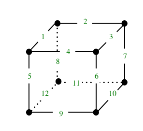
Figure 6. The associated grid graph of the $2\times 2\times 2$ box.

We compute the following

1. $I_{G_{R}}=\langle\;y_{1}y_{3}-y_{2}y_{4},\;y_{3}y_{10}-y_{6}y_{7},\;y_{4}y_{9}-y_{5}y_{6},\;y_{1}y_{12}-y_{5}y_{8},\;y_{2}y_{11}-y_{7}y_{8},\;y_{9}y_{11}-y_{10}y_{12},\;y_{2}y_{5}y_{10}-y_{1}y_{9}y_{7},\;y_{4}y_{7}y_{12}-y_{3}y_{5}y_{11},\;y_{2}y_{6}y_{12}-y_{3}y_{8}y_{9},\;y_{1}y_{6}y_{11}-y_{4}y_{8}y_{10}\;\rangle$
   

2. $I_{R_{tiling}}=\langle\;y_{2}y_{5}y_{6}y_{11}-y_{5}y_{6}y_{7}y_{8},\;y_{4}y_{9}y_{7}y_{8}-y_{5}y_{6}y_{7}y_{8},\;y_{2}y_{4}y_{9}y_{11}-y_{4}y_{9}y_{7}y_{8},\;y_{2}y_{4}y_{9}y_{11}-y_{2}y_{4}y_{10}y_{12},\;y_{1}y_{3}y_{10}y_{12}-y_{2}y_{4}y_{10}y_{12},\;y_{1}y_{3}y_{10}y_{12}-y_{1}y_{3}y_{9}y_{11},\;y_{1}y_{3}y_{10}y_{12}-y_{1}y_{6}y_{11}y_{12},\;y_{1}y_{3}y_{10}y_{12}-y_{3}y_{5}y_{8}y_{10}\rangle$
   

3. $I_{R_{flip}}=\langle\;y_{1}y_{3}-y_{2}y_{4},\;y_{3}y_{10}-y_{6}y_{7},\;y_{4}y_{9}-y_{5}y_{6},\;y_{1}y_{12}-y_{5}y_{8},\;y_{2}y_{11}-y_{7}y_{8},\;y_{9}y_{11}-y_{10}y_{12}\;\rangle.$

For this example, while $I_{R_{flip}}\neq I_{{G}_{R}}$, we do have that $I_{R_{tiling}}\subseteq I_{R_{flip}}$. This can be seen by noticing that every generator of $I_{R_{tiling}}$ is a monomial multiple of an element in $I_{R_{flip}}$. Since $I_{R_{tiling}}\subseteq I_{R_{flip}}$, the tiling space $\mathcal{T}_{R}$ is flip connected by Theorem 3.12.

Example 3.15.

In this example, let $R=B_{3,4}$, the $3\times 4$ box. The associated grid graph with edge labels is depicted in Figure 7.

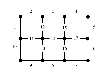
Figure 7. The grid graph associated with the $3\times 4$ box with edges labeled $1$ through $17$.

We compute the following

1. $I_{G_{R}}=\langle\;y_{1}y_{12}-y_{2}y_{11},\;y_{12}y_{15}-y_{3}y_{14},\;y_{5}y_{15}-y_{4}y_{17},\;y_{10}y_{13}-y_{9}y_{11},\;y_{13}y_{16}-y_{8}y_{14},\;y_{6}y_{16}-y_{7}y_{17},\;y_{1}y_{3}y_{9}y_{16}-y_{2}y_{8}y_{10}y_{15},\;y_{4}y_{6}y_{8}y_{12}-y_{3}y_{5}y_{7}y_{13},\;y_{1}y_{3}y_{5}y_{7}y_{9}-y_{2}y_{4}y_{6}y_{8}y_{10}\;\rangle$
   

2. $I_{R_{tiling}}=\langle\;y_{1}y_{5}y_{7}y_{9}y_{12}y_{15}-y_{2}y_{4}y_{7}y_{9}y_{11}y_{17},\;y_{1}y_{5}y_{7}y_{9}y_{12}y_{15}-y_{2}y_{4}y_{6}y_{8}y_{10}y_{14},\;y_{1}y_{5}y_{7}y_{9}y_{12}y_{15}-y_{1}y_{3}y_{5}y_{7}y_{9}y_{14},\;y_{1}y_{5}y_{7}y_{9}y_{12}y_{15}-y_{2}y_{4}y_{6}y_{10}y_{13}y_{16},\;y_{2}y_{5}y_{9}y_{7}y_{11}y_{15}-y_{1}y_{3}y_{5}y_{7}y_{9}y_{14},\;y_{2}y_{5}y_{9}y_{7}y_{11}y_{15}-y_{2}y_{4}y_{6}y_{9}y_{11}y_{16},\;y_{2}y_{4}y_{6}y_{9}y_{11}y_{16}-y_{1}y_{4}y_{7}y_{9}y_{12}y_{17},\;y_{1}y_{4}y_{7}y_{9}y_{12}y_{17}-y_{1}y_{4}y_{6}y_{9}y_{12}y_{16},\;y_{1}y_{4}y_{6}y_{9}y_{12}y_{16}-y_{2}y_{4}y_{7}y_{10}y_{13}y_{17},\;y_{2}y_{4}y_{7}y_{10}y_{13}y_{17}-y_{2}y_{5}y_{7}y_{10}y_{13}y_{15}\rangle$
   

3. $I_{R_{flip}}=\langle\;y_{1}y_{12}-y_{2}y_{11},\;y_{12}y_{15}-y_{3}y_{14},\;y_{5}y_{15}-y_{4}y_{17},\;y_{10}y_{13}-y_{9}y_{11},\;y_{13}y_{16}-y_{8}y_{14},\;y_{6}y_{16}-y_{7}y_{17}\;\rangle$.
   

In this example, as with the previous example, $I_{R_{flip}}\neq I_{{G}_{R}}$, but $I_{R_{tiling}}\subseteq I_{R_{flip}}$, hence, the tiling space $\mathcal{T}_{R}$ is flip connected by Theorem 3.12.

Example 3.16.

Let $R$ be the 3-dimensional region whose associated graph is pictured in Figure 8.

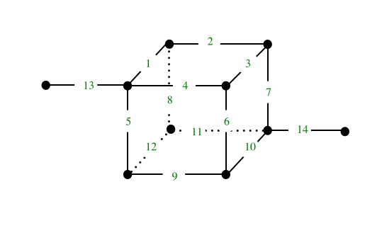
Figure 8. The labeled graph $G_{R}$ of a $3$-dimensional region $R$ that contains the $2\times 2\times 2$ cube as a subregion.

We compute the following

1. $I_{G_{R}}=\langle\;y_{1}y_{3}-y_{2}y_{4},\;y_{3}y_{10}-y_{6}y_{7},\;y_{4}y_{9}-y_{5}y_{6},\;y_{1}y_{12}-y_{5}y_{8},\;y_{2}y_{11}-y_{7}y_{8},\;y_{9}y_{11}-y_{10}y_{12},\;y_{2}y_{5}y_{10}-y_{1}y_{9}y_{7},\;y_{4}y_{7}y_{12}-y_{3}y_{5}y_{11},\;y_{2}y_{6}y_{12}-y_{3}y_{8}y_{9},\;y_{1}y_{6}y_{11}-y_{4}y_{8}y_{10}\;\rangle$
   

2. $I_{R_{tiling}}=\langle\;y_{2}y_{6}y_{12}y_{13}y_{14}-y_{3}y_{9}y_{8}y_{13}y_{14}\;\rangle$
   

3. $I_{R_{flip}}=\langle\;y_{1}y_{3}-y_{2}y_{4},\;y_{3}y_{10}-y_{6}y_{7},\;y_{4}y_{9}-y_{5}y_{6},\;y_{1}y_{12}-y_{5}y_{8},\;y_{2}y_{11}-y_{7}y_{8},\;y_{9}y_{11}-y_{10}y_{12}\;\rangle.$
   

In this example, there are only two tilings of $R$ and thus $I_{R_{tiling}}$ is a principal ideal. The tiling ideal is not contained in the flip ideal, and hence, the tiling space is not flip connected. Indeed, a trit move is needed to connect the space, which can be seen by noting that the single generator of $I_{R_{tiling}}$ can be factored into a monomial and cubic trit binomial

$$y_{13}y_{14}(y_{2}y_{6}y_{12}-y_{3}y_{9}y_{8}).$$

3.3. Tiling binomials in terms of cycle covers

Recall that for two tilings $T_{1}$ and $T_{2}$ of $R$, their union $T_{1}\cup T_{2}$ is a cycle cover of $G_{R}$. In this section, we state and prove a lemma regarding such cycle covers that will be helpful in giving an algebraic proof of Theorem 2.3.

Let $T_{1}$ and $T_{2}$ be two tilings of a cubiculated region $R$ with corresponding cycle cover $T_{1}\cup T_{2}=\mathcal{C}=\{\mathcal{C}_{1},\ldots,\mathcal{C}_{r}\}$ of $G_{R}$. We define the cycle binomial $B_{\mathcal{C}_{i}}$ corresponding to the cycle $\mathcal{C}_{i}$ as follows. Construct a closed walk $w_{i}$ on each $\mathcal{C}_{i}\in\mathcal{C}$ by starting with an edge in $T_{1}$ and then walking in either direction. Then the cycle binomial $B_{\mathcal{C}_{i}}$ is the binomial arising from the walk $w_{i}$:

$$B_{\mathcal{C}_{i}}:=B_{w_{i}}=\prod_{e\in T_{1}\cap\mathcal{C}_{i}}y_{e}-\prod_{e\in T_{2}\cap\mathcal{C}_{i}}y_{e}.$$

Lemma 3.17.

Let $T_{1}$ and $T_{2}$ be two tilings of a cubiculated region $R$ with corresponding cycle cover $T_{1}\cup T_{2}=\mathcal{C}=\{\mathcal{C}_{1},\ldots,\mathcal{C}_{r}\}$ of $G_{R}$. Then $B_{T_{1},T_{2}}$ can be written as the sum of $r$ binomials where the $i$th binomial can be factored into a monomial and the cycle binomial $B_{\mathcal{C}_{i}}$.

Proof.

We begin by describing the $i$th monomial that appears in the sum described by the lemma. Let

$$m_{1}=y^{T_{1}\setminus\mathcal{C}_{1}},$$

and for $i=2,\ldots,r$, let

$$m_{i}=y^{(T_{1}\setminus(\mathcal{C}_{1}\cup\cdots\cup\mathcal{C}_{i}))\bigcup(T_{2}\cap(\mathcal{C}_{1}\cup\cdots\cup\mathcal{C}_{i-1}))}.$$

Then, we can write $B_{T_{1},T_{2}}$ as

$$B_{T_{1},T_{2}}=m_{1}B_{\mathcal{C}_{1}}+m_{2}B_{\mathcal{C}_{2}}+\cdots+m_{r}B_{\mathcal{C}_{r}}.$$

∎

Remark 3.18.

Note that the binomial arising from a $2$-cycle $\mathcal{C}_{i}$ has the following form

$$y_{j}-y_{j}.$$

Therefore adding $B_{\mathcal{C}_{i}}$ is equivalent to adding zero. Thus, we can obtain a similar statement to Lemma 3.17 by letting $\mathcal{C}$ be all cycles of $T_{1}\cup T_{2}$ of length greater than 2.

Example 3.19.

Let $R$ be the $2\times 5$ box and consider the two tilings $T_{1}$ and $T_{2}$ pictured in Figure 9. The cycle cover $\mathcal{C}=\{\mathcal{C}_{1},\mathcal{C}_{2}\}$ of $G_{R}$ induced by $T_{1}\cup T_{2}$ is also shown in Figure 9.

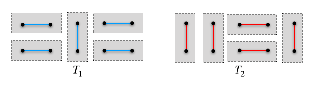
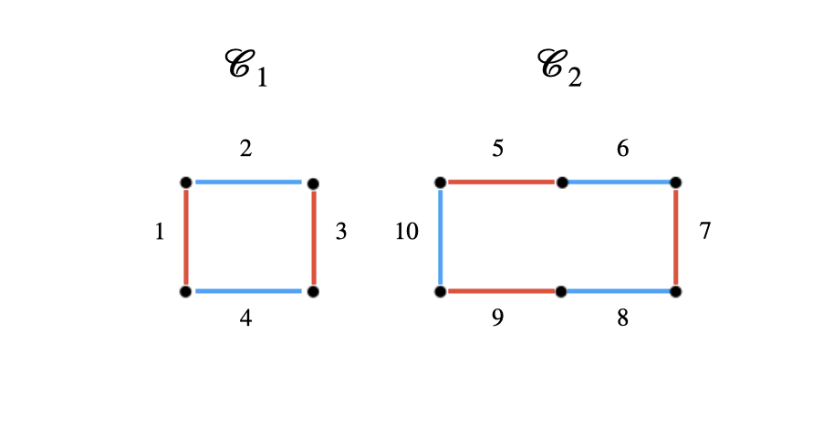
Figure 9. The top row shows two tilings, $T_{1}$ and $T_{2}$, of the $2\times 5$ box. The bottom row shows the two cycles formed when taking the union of $T_{1}$ and $T_{2}$ as edge sets of $G_{R}$.

The binomial arising from $(T_{1},T_{2})$ is

$$B_{T_{1},T_{2}}=y_{1}y_{3}y_{5}y_{7}y_{9}-y_{2}y_{4}y_{6}y_{8}y_{10}.$$

Using Lemma 3.17, we can write $B_{T_{1},T_{2}}$ in terms of $B_{\mathcal{C}_{1}}=y_{1}y_{3}-y_{2}y_{4}$ and $B_{\mathcal{C}_{2}}=y_{5}y_{7}y_{9}-y_{6}y_{8}y_{10}$ as follows

$$B_{T_{1},T_{2}}=y_{5}y_{7}y_{9}(y_{1}y_{3}-y_{2}y_{4})+y_{2}y_{4}(y_{5}y_{7}y_{9}-y_{6}y_{8}y_{10}).$$

Notice that the factored monomials in this sum have the form described in the proof of Lemma 3.17. In particular, working on the labels of the indeterminates appearing in each monomial, we have

$$\{5,7,9\}=T_{1}\setminus\mathcal{C}_{1}=\{1,3,5,7,9\}\setminus\{1,2,3,4\},$$

and

$$\{2,4\}=(T_{1}\setminus(\mathcal{C}_{1}\cup C_{2}))\cup(T_{2}\cap\mathcal{C}_{1})=\emptyset\cup(T_{2}\cap\mathcal{C}_{1})=\{2,4,6,8,10\}\cap\{1,2,3,4\}.$$

4. Connectivity of Tilings of $2$-Dimensional Regions

We conclude this paper by showing any binomial arising from two tilings of a $2$-dimensional simply connected cubiculated region $R$ is generated by quadratics. This allows us to prove that the space of tilings of $R$ is flip connected.

Definition 4.1.

A region $R$ is said to be simply connected if any simple closed curve can be shrunk to a point continuously in the set.

Remark 4.2.

A $2$-dimensional region is simply connected if it has no holes.

Theorem 4.3.

Let $R$ be a $2$-dimensional simply connected cubiculated region. Any binomial arising from two distinct tilings of $R$ is generated by quadratics. In particular, $I_{R_{tiling}}\subseteq I_{R_{flip}}.$

Our proof of Theorem 4.3 relies on a couple of lemmas that we will prove first.

Definition 4.4.

Let $R$ be a $2$-dimensional simply connected cubiculated region with graph $G_{R}$. We call a cycle $\mathcal{C}_{1}$ of $G_{R}$ a contractible cycle if, when $G_{R}$ is drawn in the plane as a grid graph, the interior of $\mathcal{C}_{1}$ contains no vertices.

Contractible cycles can be regarded as Hamiltonian cycles of a subgraph $G_{R^{\prime}}$ of $G_{R}$ where $R^{\prime}$ is a simply connected subregion of $R$. Indeed, if $R$ is simply connected, then any Hamiltonian cycle of $G_{R}$ is a contractible cycle. Moreover, when $R$ is a $2$-dimensional simply connected region, any $2$-cycle of $G_{R}$ is a contractible cycle.

Definition 4.5.

Let $R$ be a $2$-dimensional simply connected cubiculated region with graph $G_{R}$. We call a cycle $\mathcal{C}_{0}$ of $G_{R}$ a perimeter cycle if, when $G_{R}$ is drawn in the plane as a grid graph, the interior of $\mathcal{C}_{0}$ contains no cycles or only $2$-cycles. (The name perimeter comes from that fact that if $T_{1}\cup T_{2}$ contains a single perimeter cycle and no other cycles besides $2$-cycles, then the tilings $T_{1}$ and $T_{2}$ only differ on the perimeter of a simply connected subregion.)

Note that a contractible cycle is a perimeter cycle, and thus, a $2$-cycle is a perimeter cycle.

Lemma 4.6.

Let $T_{1}$ and $T_{2}$ be two tilings of a simply connected $2$-dimensional cubiculated region $R$ such that $T_{1}\cup T_{2}$ is a collection of perimeter cycles $\mathcal{C}_{1},\ldots,\mathcal{C}_{r}$. There exists a sequence of flip moves $(D_{1_{1}},D_{2_{1}}),\ldots,(D_{1_{s}},D_{2_{s}})$ that takes $T_{1}$ to $T_{1}^{\prime}$ and a sequence of flip moves $(D^{\prime}_{1_{1}},D^{\prime}_{2_{1}}),\ldots,(D^{\prime}_{1_{t}},D^{\prime}_{2_{t}})$ that takes $T_{2}$ to $T_{2}^{\prime}$ such that $T_{1}^{\prime}\cup T_{2}^{\prime}$ is a collection of contractible cycles. In particular,

$$B_{T_{1},T_{2}} =y^{T_{1}\setminus D_{1_{1}}}(y^{D_{1_{1}}}-y^{D_{2_{1}}})+\ldots+y^{T_{1}^{\prime}\setminus D_{2_{s}}}(y^{D_{1_{s}}}-y^{D_{2_{s}}})$$

$$+B_{T_{1}^{\prime},T_{2}^{\prime}}$$

$$+y^{T_{2}^{\prime}\setminus D^{\prime}_{2_{t}}}(y^{D^{\prime}_{2_{t}}}-y^{D^{\prime}_{1_{t}}})+\ldots+y^{T_{2}\setminus D^{\prime}_{1_{1}}}(y^{D^{\prime}_{2_{1}}}-y^{D^{\prime}_{1_{1}}})$$

where each binomial of the form $y^{D_{1_{i}}}-y^{D_{2_{i}}}$ or $(y^{D_{2_{i}}}-y^{D_{1_{i}}})$ has degree $2$.

Proof.

Let $k$ be the number of vertices contained in the interiors of $\mathcal{C}_{1},\ldots,\mathcal{C}_{r}$ when $G_{R}$ is drawn in the plane as a grid graph. We will induct on $k$.

For the base case, assume $k=0$. Then $\mathcal{C}_{1},\ldots,\mathcal{C}_{r}$ are all contractible cycles. Therefore, $T_{1}\cup T_{2}$ is a collection of contractible cycles.

Now suppose the statement is true for up to $k-1$ internal vertices and assume the cycles in $\mathcal{C}$ have $k>0$ internal vertices. Since $k>0$, the interior of at least one of $\mathcal{C}_{1},\ldots,\mathcal{C}_{r}$ contains at least one 2-cycle, let’s assume $\mathcal{C}_{1}$ contains at least one 2-cycle. We will consider three cases based on the positions of the interior $2$-cycles.

Case 1: An interior $2$-cycle is parallel to $\mathcal{C}_{1}$.

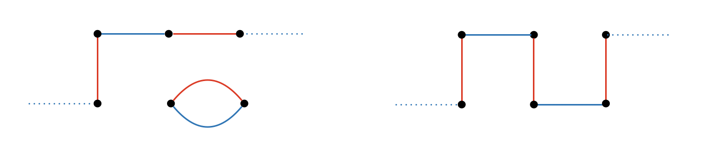
Figure 10. A local flip is performed on with the $2$-cycle parallel to $\mathcal{C}_{1}$.

In this case we can perform a local flip the edge parallel to the $2$-cycle as shown in Figure 10. This yields a decrease in the number of internal vertices by $2$, and then, we can apply the induction hypothesis.

Case $2$: There exists an interior $2$-cycle that is not parallel to $\mathcal{C}_{1}$.

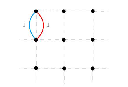
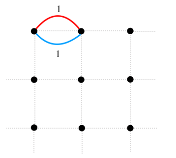
Figure 11. On the left is a north-south 2-cycle. On the right is an east-west $2$-cycle.

  
Let us categorize $2$-cycles into two types: north-south cycles and east-west cycles (see Figure 11). In the case where there is no $2$-cycle parallel to $\mathcal{C}_{1}$, then (i) there exists a east-west cycle such that the two vertices in $G_{R}$ directly north of the $2$-cycle or the two vertices in $G_{R}$ directly south of the $2$-cycle are both contained in $\mathcal{C}_{1}$ or (ii) there exists a north-south cycle such that the two vertices in $G_{R}$ directly east of the $2$-cycle or the two vertices in $G_{R}$ directly west of the $2$-cycle are both contained in $\mathcal{C}_{1}$. We note that if either $(i)$ or $(ii)$ does not hold, then starting at any interior $2$-cycle, there is an infinite sequence of $2$-cycles that can be constructed by choosing the $2$-cycle that covers at least one vertex to the north or east of the previous cycle, and thus $R$ is not finite.

Without loss of generality, let’s assume that there is a $2$-cycle $\mathcal{C}_{2}$ of the form described in situation (i) such that the two vertices directly north of the $\mathcal{C}_{2}$ are both contained in $G_{R}$. In this situation, $\mathcal{C}_{1}$ must transverse the vertices north of $\mathcal{C}_{2}$ in the way illustrated in Figure 12. Note that the edges $e_{1}$ and $e_{2}$ in Figure 12 must be from the same tiling since every chord of $\mathcal{C}_{1}$ must be even. After performing a local flip, $\mathcal{C}_{1}$ is split into two cycles, $\mathcal{C}_{1}^{\prime}$ that contains $\mathcal{C}_{2}$ and $\mathcal{C}_{2}^{\prime}$ that contains no vertices or only $2$-cycles and thus is a new perimeter cycle; see Figure 13. We have not reduced the number of interior vertices, however, we now meet the conditions of Case 1 and can proceed accordingly.

∎

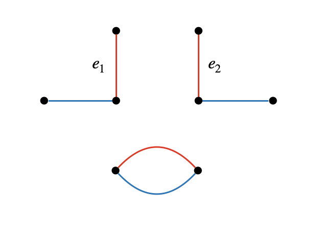
Figure 12. An east-west cycle such that the two vertices in $G_{R}$ directly north of the $2$-cycle are traversed by $\mathcal{C}_{1}$.

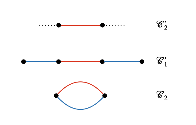
Figure 13. Configuration from Figure 12 after performing a local flip.

Lemma 4.7.

Let $R$ be a simply connected $2$-dimensional cubiculated region and let $T_{1},T_{2}$ be two tilings such that $T_{1}\cup T_{2}$ contains a single contractible cycle of $G_{R}$ of length $\geq 4$ and no other cycles besides $2$-cycles. Then $B_{T_{1},T_{2}}$ is generated by quadratics.

Proof.

Let $\mathcal{C}_{1}$ be the single contractible cycle of length $\geq 4$. We will proceed by induction on the length of $\mathcal{C}_{1}$, which we will denote by $k$.

For the base case, let $k=4$. Then $\mathcal{C}_{1}$ is a single $4$-cycle. Let $\mathcal{C}_{1}$ be labeled as in Figure 14, then $B_{T_{1},T_{2}}$ is the product of a monomial and the quadratic $y_{1}y_{3}-y_{2}y_{4}$, and thus is generated by quadratics.

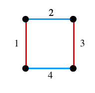
Figure 14. A single $4$-cycle.

Now assume $\mathcal{C}_{1}$ has length $k>4$ and the statement holds whenever the length of $\mathcal{C}_{1}$ is less than $k$. Embed $G_{R}$ into a grid graph and let row $i$ be the first row (scanning from north to south) that contains a vertex covered by $\mathcal{C}_{1}$ and let column $j$ be the first column in row $i$ that contains a vertex covered by $\mathcal{C}_{1}$; we will call the $(i,j)$th vertex of the grid graph, the north-west corner of $\mathcal{C}_{1}$ and refer to it as $v$.

By the way we selected the north-west corner, the vertex $v$ must be traversed by $\mathcal{C}_{1}$ as illustrated in Figure 15. Furthermore, since $R$ is simply connected, and $\mathcal{C}_{1}$ is a contractible cycle, the highlighted vertex in Figure 15 must also be covered by $\mathcal{C}_{1}$. The highlighted vertex can be covered in three ways as shown in Figure 16.

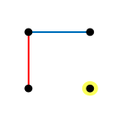
Figure 15. The north-west corner of $\mathcal{C}_{1}$.

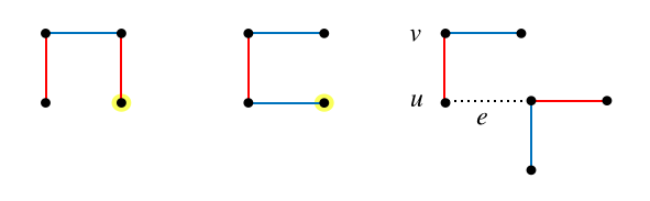
Figure 16. The three ways the north-west corner can be traversed by $\mathcal{C}_{1}$.

For the first two cases illustrated in Figure 16, we can perform a local flip move that decomposes $C_{1}$ into a $2$-cycle and a contractible cycle of length less than $\mathcal{C}_{1}$, and then apply the induction hypothesis.

For the third case illustrated in Figure 16, note that the edge $e$ in $G_{R}$ from $u$, the vertex south of $v$, to the highlighted vertex is an even chord of $\mathcal{C}_{1}$, since $G_{R}$ contains only even cycles. Using $e$, we can split $\mathcal{C}_{1}$ into two even contractible cycles, $\mathcal{C}_{2}$ and $\mathcal{C}_{3}$, that overlap on the edge $e$. Then, similar to the proof of Lemma 3.17, and assuming the edges adjacent to $e$ in $\mathcal{C}_{2}$ belong to $T_{1}$, we can define the following two pairs of tilings:

$$S_{1} =T_{1}\ \ \ \ \ S_{2} =(T_{1}\setminus\mathcal{C}_{2})\cup(\mathcal{C}_{2}\setminus T_{1})$$

$$U_{1} =(T_{1}\setminus\mathcal{C}_{2})\cup(\mathcal{C}_{2}\setminus T_{1})=(T_{2}\setminus\mathcal{C}_{3})\cup(\mathcal{C}_{3}\setminus T_{2})\ \ \ \ \ \ U_{2} =T_{2}.$$

The binomial $B_{T_{,}T_{2}}$ can be written in terms of binomials arising from $S_{1},S_{2}$ and $U_{1},U_{2}$:

$$B_{T_{1},T_{2}}=B_{S_{1},S_{2}}+B_{U_{1},U_{2}}.$$

Since $S_{1}\cup S_{2}$ and $U_{1}\cup U_{2}$ both contain only $2$-cycles and a single contractible cycle of length $\geq 4$ but less than $k$, the binomials $B_{S_{1},S_{2}}$ and $B_{U_{1},U_{2}}$ are both generated by quadratics and thus $B_{T_{1},T_{2}}$ is generated by quadratics. ∎

We now can begin our proof of Theorem 4.3. We will induct on the binomial degree of the tiling binomial.

Definition 4.8.

Let $b$ be a homogeneous binomial of the form $b=m(u-v)$ where $m,u,v$ are monomials and $\gcd(u,v)=1$. We will call the $\deg u=\deg v$, the binomial degree of $b$.

Proof of Thoerem 4.3.

Let $B_{T_{1},T_{2}}$ be a non-zero binomial arising from two tilings $T_{1},T_{2}$. We will induct on the binomial degree of $B_{T_{1},T_{2}}$.

In the base case, let’s assume the binomial degree of $B_{T_{1},T_{2}}$ is 2. Then

$$B_{T_{1},T_{2}}=y^{T_{1}\setminus D_{1}}(y^{D_{1}}-y^{D_{2}})$$

where the size of the move $(D_{1},D_{2})$ is 2 and thus a flip move.

Now, assume that the binomial degree of $B_{T_{1},T_{2}}$ is $k>2$ and the statement holds whenever the binomial degree is less than $k$. Note that the binomial degree of $B_{T_{1},T_{2}}$ is equal to $1/2$ the sum of the lengths of all cycles with length $>2$ in $T_{1}\cup T_{2}$. Thus, we can proceed by considering two cases based on whether $T_{1}\cup T_{2}$ has more than one cycle with length $>2$ or a single cycle of length $>2$.

For the first case, assume $T_{1}\cup T_{2}$ has more than one cycle with length $>2$; let’s call these cycles $\mathcal{C}_{1},\ldots,\mathcal{C}_{r}$. By Lemma 3.17, $B_{T_{1},T_{2}}$ can be written as the sum of $r$ binomials where the $i$th binomial can be factored into a monomial and the cycle binomial $B_{\mathcal{C}_{i}}$. This means that the $i$th binomial in the sum has binomial degree equal to $1/2\cdot$(length of $\mathcal{C}_{i}$), which is less than $k$. Thus, by applying the induction hypothesis to each binomial in the sum, we have that $B_{T_{1},T_{2}}$ is generated by quadratics and $B_{T_{1},T_{2}}\in I_{flip}$.

For the second case, assume $T_{1}\cup T_{2}$ has a single cycle $\mathcal{C}_{1}$ with length $>2$. In this case, $\mathcal{C}_{1}$ is a perimeter cycle, Thus, by combining Lemma 4.6 and Lemma 3.17, and applying Lemma 4.7 to each resulting contractible cycle, we have $B_{T_{1},T_{2}}\in I_{flip}$. ∎

Corollary 4.9.

Let $R$ be a $2$-dimensional simply connected cubiculated region. Then $\mathcal{T}_{R}$ is flip connected.

References

- [1] J. Bouttier, G. Chapuy, and S. Corteel, From Aztec Diamonds to pyramid: Steep Tilings, Trans. Amer. Math. Soc. (2017), 5921–5959.
- [2] T. Chin, A computational commutative algebra approach to tilings, Applied Mathematics Theses and Dissertations. Brown Digital Repository. Brown University Library (2019).
- [3] M. Ciucu, An improved upper bound for the three dimensional dimer problem, Duke Mathematical Journal (1998), 1–11.
- [4] H. Cohn, R. Kenyon, and J. Propp, A Variational Principle for Domino Tilings, Journal of the AMS 14 (2001), 297–346.
- [5] P. Diaconis and B. Sturmfels, Algebraic algorithms for sampling from conditional distributions, The Annals of Statistics 26 (1998), no. 1, 363–397.
- [6] M. Drton, B. Sturmfels, and S. Sullivant, Lectures on algebraic statistics, vol. 39, Springer Science & Business Media, 2008.
- [7] H.D. Ebbinghaus, Computation Theory and Logic. Lecture Notes in Computer Science, 1987.
- [8] M. Fisher and H. Temperley, The Dimer Problem in Statistical Mechanics–an Exact Result, Philosophical Magazine (1961), 1061–1063.
- [9] R.H. Fowler and G.S. Rushbrooke, Statistical theory of perfect solutions, Transactions of Faraday Society (1937), 1272–1294.
- [10] J. Freire, C. Klivans, P. Milet, and N. Saldanha, On the Connectivity of Spaces of Three-dimensional Domino Tilings, arXiv preprint arXiv:1702.00798 (2017).
- [11] F. Galetto, J. Hofscheier, G. Keiper, C. Kohne, A. Van Tuyl, M. Paczka, and E. Uribe, Betti numbers of toric ideals of graphs: A case study, Journal of Algebra and Its Applications 18 (2019), no. 12, 1950226.
- [12] and A. Van Tuyl J. Biermann, A. O’Keefe, Bounds on the regularity of toric ideals of graphs, Advances in Applied Mathematics 85 (2017), 84–102.
- [13] P. Kasteleyn, The Statistics of Dimers on a Lattice I. The Number of Dimer Arrangements on a Quadratic Lattice, Physica 27 (1961), 1209–1225.
- [14] R. Kenyon and A. Okounkov, Planar dimers and Harnack curves, Duke Mathematical Journal (2006), 499–524.
- [15] P.H. Milet and N.C. Saldanha, Domino Tilings of Three-dimensional Regions: flips, trits and twists, (2014).
- [16] H. Ohsugi and T. Hibi, Toric Ideals Generated by Quadratic Binomials, Journal of Algebra 218 (2009), 509–527.
- [17] by same author, Toric Ideals and their Circuits, Journal of Commutative Algebra 5 (2012), 309–322.
- [18] R. Kenyon A. Okounkov and S. Sheffield, Dimers and amoebae, Annals of Mathematics (2006), 1019–1056.
- [19] J. Propp and R. Stanley, Domino tilings with barriers, Journal of Combinatorial Theory, Series A (1999), 347–366.
- [20] D. Randall and G. Yngve, Random three-dimensional Domino Tilings of Aztec octahedra and tetrahedra: An Extension of Domino Tilings, Proceedings of the eleventh annual ACM-SIAM symposium on Discrete Algorithms (2000), 207–233.
- [21] E. Reyes, C. Tatakis, and A. Thoma, Minimal generators of toric ideals of graphs, Advances in Applied Mathematics 48 (2012), no. 1, 64–78.
- [22] N.C. Saldanha, C. Tomei, M.A. Casarin Jr, and D. Romualdo, Spaces of Domino Tilings, Discrete and Computational Geometry (1995), 207–233.
- [23] R. Stanley, What is enumerative combinatorics?, Springer, 1986.
- [24] C. Tatakis and A. Thoma, On the universal gröbner bases of toric ideals of graphs, Journal of Combinatorial Theory, Series A 118 (2011), no. 5, 1540–1548.
- [25] W. Thurston, Conway’s Tiling Groups, The American Mathematical Monthly (1990), 757–773.
- [26] R. Villareal, Monomial Algebras, 2nd ed., CRC Press, 2015.
- [27] D. West, Introduction to Graph Theory, 2nd ed., Pearson, 2015.