General Initial Value Problem for the Nonlinear Shallow Water Equations: Runup of Long Waves on Sloping Beaches and Bays

Abstract

We formulate a new approach to solving the initial value problem of the shallow water-wave equations utilizing the famous Carrier-Greenspan transformation [G. Carrier and H. Greenspan, J. Fluid Mech. 01, 97 (1957)]. We use a Taylor series approximation to deal with the difficulty associated with the initial conditions given on a curve in the transformed space. This extends earlier solutions to waves with near shore initial conditions, large initial velocities, and in more complex U-shaped bathymetries; and allows verification of tsunami wave inundation models in a more realistic 2-D setting.

I Introduction

Tsunami modeling and forecast is an important scientific problem impacting coastal communities worldwide. Many models for tsunami wave propagation use the 2+1 shallow water equations (SWE), an approximation of the Navier-Stokes equation Kanoglu et al. (2015). These numerical models must be continuously verified and validated to ensure the safety of coastal communities and infrastructure NTHMP (2012). Apart from verification against data from actual tsunami events, numerical models are also extensively verified against analytical solutions of the 2+1 SWE which exist for idealized bathymetries Synolakis et al. (2008). These analytical solutions also give important qualitative insight to tsunami run-up and amplification.

Typically, the process of tsunami generation is considered as an instant vertical motion of the sea bottom ignoring the water velocities in the source. However, incorporation of the water velocities into the initial conditions is important from physical point of view, see for instance Kanoglu and Synolakis (2006). For a more complete analysis of tsunami hydrodynamics, modeling and forecast, we refer the reader to Synolakis and Bernard (2006); Synolakis et al. (2008); Kanoglu et al. (2015); NTHMP (2012); Kanoglu and Synolakis (2015).

A classical example of an analytical solution for the 2+1 SWE is computing the run-up of long-waves on a sloping beach Synolakis (1987). Because of the symmetric bathymetry, the 2+1 SWE reduce to the 1+1 SWE, which could be solved directly in the physical space Antuono and Brocchini (2010) or in the new coordinates using the Carrier-Greenspan transformation Carrier and Greenspan (1957). The SWE in the transformed coordinates has been extensively studied as an initial value problem (IVP) Carrier et al. (2003); Kanoglu (2004); Kanoglu and Synolakis (2006); Harris et al. (2015a); Aydin and Kanoglu (2017) and as a boundary value problem Synolakis (1987); Antuono and Brocchini (2007). The IVP for waves with non-zero initial velocity have been previously derived using a Green’s function in Carrier et al. (2003); Kanoglu and Synolakis (2006), though both solutions imply assumptions regarding the initial velocity as discussed later. Thus, the complete and exact solution to the IVP for waves with nonzero initial velocities remains a long standing open problem Tuck and Hwang (1972); Kanoglu and Synolakis (2006); Antuono and Brocchini (2007).

The 1+1 SWE for the sloping beach have recently been generalized to model waves in sloping narrow channels using the cross-sectionally averaged 1+1 SWE Zahibo et al. (2006). Furthermore, the hodograph transform given by Carrier and Greenspan (1957) can be generalized to sloping bays with arbitrary cross sections, allowing a much richer problem to study Rybkin et al. (2014). Though the cross-sectionally averaged 1+1 SWE have no analytical solution for bays with arbitrary cross sections, an analytical solution exists for symmetric U-shaped bays, i.e bays with a cross section $z\propto y^{m}$ Zahibo et al. (2006); Rybkin et al. (2014); Anderson et al. (2017). The known solution for sloping beaches is an asymptotic solution of such bays when $m\rightarrow\infty$.

In this letter we propose a new approach to solve the IVP for the cross-sectionally averaged 1+1 SWE in U-shaped bays for waves with arbitrary initial velocities exactly. Our solution uses a Taylor expansion to deal with the initial data given on a curve (under the Carrier-Greenspan transformation the line $t=0$ is mapped to a curve in the transformed plane), a problem that was not sufficiently treated in the previous solutions. This allows run-up computation of near shore long waves, unlike the previous IVP solutions that require the initial wave to be far from shore Kanoglu and Synolakis (2006). Additionally, we present some qualitative geophysical implications using this new solution.

II Solution of the IVP

The cross-sectionally averaged 1+1 SWE for U-shaped bays describe the evolution of long waves in a sloping narrow bay with an unperturbed water height $h(x)=x$ along the main axis of the bay in dimensionless form. The wave is assumed to propagate uniformly through the bay in the $x$ direction, a valid assumption as shown in Shimozono and Takenori (2016); Anderson et al. (2017). The cross-sectionally averaged SWE for such bays in dimensionless form are given by Zahibo et al. (2006); Anderson et al. (2017) to be

$$\eta_{t}+u(1+ \eta_{x} )+\beta^{2}(x+\eta)u_{x}=0,$$ (1a)

$$u_{t} + uu_{x}+\eta_{x}=0,$$ (1b)

where $u(x,t)$ and $\eta(x,t)$ are the horizontal depth-averaged velocity and free-surface elevation along the main axis of the bay, respectively, and $\beta^{2}=m/(m+1)$ is the wave propagation speed along a constant depth channel. An arbitrary scaling parameter $l$ is used to introduce the dimensionless variables $x=\tilde{x}/l$, $\eta=\tilde{\eta}/(l\alpha)$, $u=\tilde{u}/\sqrt{g\alpha l}$ and $t=\tilde{t}\sqrt{g\alpha/l}$. Here $\tilde{x},\tilde{t},\tilde{\eta}$ and $\tilde{u}$ are the dimensional variables, $g$ is the gravitational acceleration, and $\alpha$ is the slope of the incline.

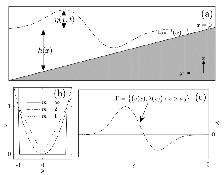
Figure 1: Definition sketch: (a) $x-z$ cross section with perturbed and unperturbed water heights, not to scale. (b) $y-z$ cross section of a plane beach where $m=\infty$, a parabolic bay where $m=2$, and a V-shaped bay where $m=1$. (c) The curve $\Gamma$ on which the initial conditions are prescribed in the transformed space for the wave shown in (a), not to scale.

We use the form of the Carrier-Greenspan transformation presented in Tuck and Hwang (1972),

$$\varphi=u,\ \psi=\eta+\frac{u^{2}}{2}$$ (2a)

$$s=x+ \eta,\ \ \ \ \ \ \ \ \ \lambda=t-u,$$ (2b)

to reduces (1) to the linear system

$$\Phi_{\lambda}+A(s)\Phi_{s}+B\Phi=0,$$ (3)

where $\Phi(s,\lambda)=\begin{pmatrix}\varphi(s,\lambda)\\ \psi(s,\lambda)\end{pmatrix}$, $A(s)=\begin{pmatrix}0&1\\ \beta^{2}s&0\end{pmatrix}$, and $B=\begin{pmatrix}0&0\\ 1&0\end{pmatrix}$. This form of the Carrier-Greenspan transformation has two useful properties, the moving shoreline is fixed at $s=0$ and the resulting linear system, (3), is the linear SWE. For comparison to other texts, specifically Kanoglu and Synolakis (2006); Rybkin et al. (2014); Carrier and Greenspan (1957); Synolakis (1987), the transform variable $\sigma=2\sqrt{s}/\beta$ is typically used, along with the introduction of a potential function to form a single linear second order partial differential equation.

We consider (3) with the general initial conditions in physical space $\eta(x,0)=\eta_{0}(x)$ and $u(x,0)=u_{0}(x)$. Under transformation (2b), $\eta_{0}(x)$ and $u_{0}(x)$ transform into initial conditions on a parameterized curve $\Gamma$ in the $(s,\lambda)$ plane, depicted in Fig. 1c, which leads to a non-trivial IVP. It is natural to parameterize this curve using the coordinate $x$, $\Gamma=\{\Gamma(x):x>x_{0}\}$, where

$$\Gamma(x)=\big{(}s(x),\lambda(x)\big{)}=\big{(}x+\eta_{0}(x),-u_{0}(x)\big{)},$$ (4)

and $x_{0}$ is the $x$ position of the shoreline at time $t=0$. The initial condition is then given by

$$\Phi|_{\Gamma(x)}=\Phi_{0}(x)=\begin{pmatrix}u_{0}(x)\\ \eta_{0}(x)+u_{0}^{2}(x)/2\end{pmatrix}.$$ (5)

A general solution to (3) can be found using the Hankel transform to be Zahibo et al. (2006); Anderson et al. (2017)

$$\psi(s,\lambda) = s^{-\frac{1}{2m}}\int_{0}^{\infty}\left\{a(k)\cos(\beta k\lambda)+b(k)\sin(\beta k\lambda)\right\}$$ (6a)

$$\times J_{1/m}\left(2k\sqrt{s}\right)dk,$$

$$\varphi(s,\lambda) = \frac{1}{\beta}s^{-\frac{1}{2m}-\frac{1}{2}}\int_{0}^{\infty}\left\{a(k)\sin(\beta k\lambda)-b(k)\cos(\beta k\lambda)\right\}$$ (6b)

$$\times J_{1/m+1}\left(2k\sqrt{s}\right)dk,$$

where $J_{\nu}(\alpha)$ is the Bessel function of the first kind of order $\nu$, and $a(k)$ and $b(k)$ are arbitrary functions determined by the initial conditions. We note that the apparent singularities at $s=0$ are removed using the asymptotic of the Bessel function of the first kind around zero.

In the piston model of generation, i.e. with zero initial velocity, the curve $\Gamma$ coincides with the line $\lambda=0$. For arbitrary initial conditions on the line $\lambda=0$, using the inverse Hankel transform, we have that

$$a(k) = 2k\int_{0}^{\infty}\psi(s_{*},0)s_{*}^{\frac{1}{2m}}J_{\frac{1}{m}}\left(2k\sqrt{s_{*}}\right)ds_{*},$$ (7a)

$$b(k) = -2\beta k\int_{0}^{\infty}\varphi(s_{*},0)s_{*}^{\frac{1}{2m}+\frac{1}{2}}J_{\frac{1}{m}+1}\left(2k\sqrt{s_{*}}\right)ds_{*}.\ \ \ \ \ \ \ \$$ (7b)

For waves with zero initial velocity, using (5) and a simple change of variables, (7) simplifies to $b(k)=0$, and

$$a(k)=2k\int_{x_{0}}^{\infty} \eta_{0}(x_{*})\big{(}x_{*}+\eta_{0}(x_{*})\big{)}^{\frac{1}{2m}}J_{\frac{1}{m}}\left(2k\sqrt{x_{*}+\eta_{0}(x_{*})}\right)$$ (8)

$$\times(1+\eta_{0}^{\prime}(x_{*}))dx_{*},$$

where primes denote derivatives in $x$. Using (6), $\varphi(s,\lambda)$ and $\psi(s,\lambda)$ can be computed . The solution is then transformed to physical space using (2). The solution over a large number of grid points can be found by interpolation using Delaunay triangulation, as in Anderson et al. (2017). Alternatively, Newton-Raphson iterations can be used to find the solution for a particular location $x$ or time $t$, as in Synolakis (1987); Kanoglu (2004).

If the initial wave has an initial velocity, the curve $\Gamma$ may be complicated so that an exact solution does not exist. Reference Kanoglu and Synolakis (2006) used the approximation $s\approx x$ to find an approximate solution for wave run-up on plane beaches using a Green’s function. This solution is similar to (6) and (7) under the appropriate change of variables and order of integration, with $m=\infty$. Although Kanoglu and Synolakis (2006) defined the initial condition along a curve in the transform space, the obtained results are expressed as trigonometric functions of $\lambda-\lambda_{0}(s)$, where $\lambda_{0}(s)=-u_{0}(s)$. Therefore, the resulting function solves the governing partial differential equation approximately as long as ${\partial u_{0}}/{\partial x}\approx 0$. An interested reader could find further details in the Appendix. Even though approximation in Kanoglu and Synolakis (2006); Carrier et al. (2003) are applicable to many geophysical conditions, i.e. when ${\partial u_{0}}/{\partial x}\approx 0$ or $u_{0}\approx 0$, but for near shore waves with large initial velocities those solutions might break down.

To overcome this difficulty, we propose to project the initial conditions onto the line $\lambda=0$ using Taylor’s theorem. For such a projection to exist, the transformation $s=x+\eta_{0}(x)$ must be bijective, and therefore $\eta_{0}^{\prime}(x)>-1$ for all $x$. We will call the projection of the initial condition to $n^{\text{th}}$ order

$$\Phi_{n}(x)=\Phi_{n}(s(x))=\sum_{k=0}^{n}\left[\frac{(-\lambda)^{k}}{k!}\frac{\partial^{k}\Phi}{\partial\lambda^{k}}\right]_{\Gamma(x)}.$$ (9)

Once the desired $\Phi_{n}(x)$ is obtained, $a(k)$ and $b(k)$ can be computed using (7). Furthermore, a simple change of variables $s_{*}=x_{*}+\eta_{0}(x_{*})$ in the integration of $a(k)$ and $b(k)$, similar to the change of variables in (8) for waves with zero initial velocity, nullifies the need for the approximation $s\approx x$ required in the previous IVP solutions in Kanoglu and Synolakis (2006); Carrier et al. (2003). The complete solution can then be found using (2) as described above. This method allows computing the solution to any desired accuracy without assumptions on the initial velocity profile.

The partial derivatives in (9) are not explicitly computable from our initial conditions. To put (9) in explicit form we use the chain rule

$$\Phi_{0}^{\prime}=\frac{d\Phi_{0}}{dx} = (1+\eta_{0}^{\prime})\frac{\partial\Phi}{\partial s}\Big{|}_{\Gamma}-u_{0}^{\prime}\frac{\partial\Phi}{\partial\lambda}\Big{|}_{\Gamma}$$ (10)

$$= (1+\eta_{0}^{\prime})\frac{\partial\Phi}{\partial s}\Big{|}_{\Gamma}+u_{0}^{\prime}\left[A\frac{\partial\Phi}{\partial s}+B\Phi\right]_{\Gamma}$$

$$= D\frac{\partial\Phi}{\partial s}\Big{|}_{\Gamma}+u_{0}^{\prime}B\Phi\Big{|}_{\Gamma},$$

where $D=(1+\eta_{0}^{\prime})I+u_{0}^{\prime}A$, and $I$ is the $2$-by-$2$ unit matrix. Noting that

$$\Phi_{1}=\left[\Phi-\lambda\frac{\partial\Phi}{\partial\lambda}\right]_{\Gamma}=\Phi|_{\Gamma}+u_{0}\frac{\partial\Phi}{\partial\lambda}\Big{|}_{\Gamma}=\Phi|_{\Gamma}-u_{0}\left[A\frac{\partial\Phi}{\partial s}+B\Phi\right]_{\Gamma}$$

and after substituting $\Phi_{s}$ from (10), while recalling that $\Phi_{0}=\Phi|_{\Gamma}$, we obtain

$$\Phi_{1}=\Phi_{0}+u_{0}\left\{u_{0}^{\prime}AD^{-1}B\Phi_{0}-B\Phi_{0}-AD^{-1}\Phi_{0}^{\prime}\right\}.$$

Similarly, higher order terms can be found using the recursive relationship

$$\Phi_{n} = \Phi_{n-1}+\frac{(u_{0})^{n}}{n!}\left[u_{0}^{\prime}AD^{-1}B-B-AD^{-1}\frac{d}{dx}\right]^{n}\Phi_{0}$$ (11)

$$= \Phi_{n-1}+\frac{1}{n}\left[u_{0}u_{0}^{\prime}AD^{-1}B-u_{0}B+(n-1)u_{0}^{\prime}AD^{-1}\right]$$

$$\ \ \times(\Phi_{n-1}-\Phi_{n-2})-\frac{u_{0}}{n}AD^{-1}(\Phi_{n-1}^{\prime}-\Phi_{n-2}^{\prime}).$$

It is important to understand the limitations of this approach. Based on the given formulas, the projection of the initial conditions remains one-to-one so long as $D$ remains nonsingular, which corresponds to $\left(1+\eta_{0}^{\prime}\right)^{2}-(u_{0}^{\prime})^{2}\beta^{2}(x+\eta_{0})>0$ for all $x$. To simplify this condition, we define the breaking parameter to be

$$\text{Br}=\max_{x\in[x_{0},\infty)}\left\{\beta|u_{0}^{\prime}(x)|\sqrt{x+\eta_{0}(x)}-\eta_{0}^{\prime}(x)\right\}.$$

So long as $\text{Br}<1$ the projection is one-to-one. We emphasize that our solution method is only valid for initial profiles and velocities that satisfy the conditions $\text{Br}<1$ and $\eta_{0}^{\prime}>-1$. From (2b) and (1), it follows that the condition $\text{Br}<1$ is equivalent to the Jacobian of the Carrier-Greenspan transform not vanishing at $t=0$. For application purposes, typical tsunami waves have a much larger wavelength than wave height Kanoglu and Synolakis (2006), and thus satisfy $|u_{0}^{\prime}|,|\eta_{0}^{\prime}|\ll 1$. Therefore these conditions pose little restrictions for the modeling of geophysical long waves (i.e. “localized” water disturbance such as Gaussian, solitary or N-waves having the water level $\eta_{0}(x)$ and velocity $u_{0}(x)$ infinitesimal for $x\to\infty$).

III Qualitative Analysis

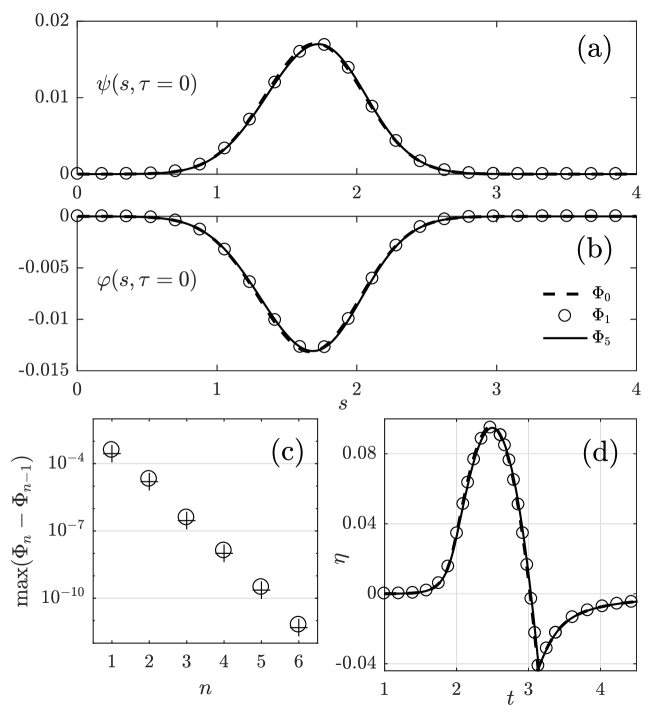
Figure 2: The transformation of an incident Gaussian wave given by (12) with $a=0.017$, $b=4.0$ and $x_{0}=1.69$. (a) $\psi(s,\lambda=0)$ to zeroth, first, and fifth order. (b) $\varphi(s,\lambda=0)$ to zeroth, first, and fifth order. (c) The maximum difference between approximations of the initial profile: $\circ$ and $+$ represent the maximum difference in $\varphi(s,\lambda=0)$and $\psi(s,\lambda=0)$, respectively. (d) Comparison of the shoreline displacement for the three orders of approximation ($n=0,1,5$) of projection of the initial conditions in (a) and (b), the line code is the same as in plot (b).

Although use of solitary waves as proxies for geophysical tsunamis is subject to the discussion Madsen et al. (2008), we seek to validate our proposed solution to the IVP by checking the convergence of the solution and comparing it to the previous solution in Kanoglu and Synolakis (2006). Reference Kanoglu and Synolakis (2006) analyzed a Gaussian initial wave profile defined by

$$\eta_{0}(x)=ae^{-b(x-x_{0})^{2}},$$ (12)

with the linear approximation of initial velocity $u_{0}(x)=-\eta_{0}(x)/\sqrt{x}$. At the same time, the developed method (9) also allows computations for the nonlinear approximation to the initial velocity $u_{0}(x)=-2(\sqrt{x+\eta_{0}}-\sqrt{x})$.

In Fig. 2a,b we present several orders of approximations for the transformation of the initial profile of such wave. We note that the iterations converge very rapidly, with the higher order approximations overlapping with the zeroth order approximation. The maximum change in the initial profile between iterations is presented in Fig. 2c. The convergence appears linear, with the difference after just six iterations approaching the machine limit. In Fig. 2d we present the shoreline run-up for several different orders of approximation. Notice that the zeroth order profile coincides almost completely with the higher order approximations. Because of this, both previous solutions Kanoglu and Synolakis (2006); Carrier et al. (2003) with assumptions ${\partial u_{0}(x)}/{\partial x}\approx 0$ or $u_{0}(x)\approx 0$, give valid results for such initial conditions. Figure 2d allows direct comparison to figure 3d in Kanoglu and Synolakis (2006).

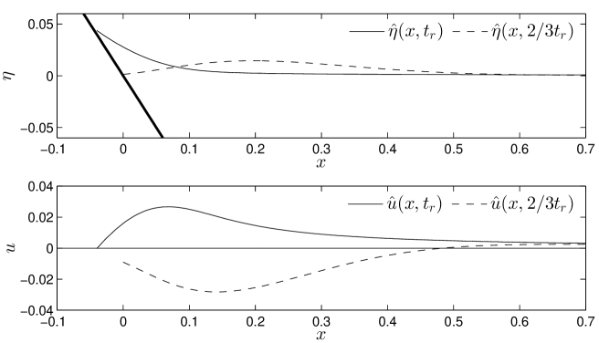
Figure 3: Profiles of the water level $\hat{\eta}$ (top) and water velocity $\hat{u}$ (bottom) for the initial condition: a zero-velocity Gaussian waves given by (12) with $a=0.017$, $b=4.0$ and $x_{0}=1.69$ running up a plane beach ($m=\infty$).

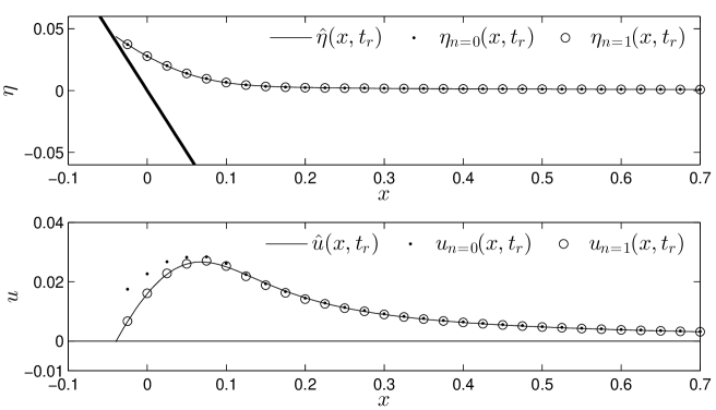
Figure 4: Comparison of the water level $\eta$ (top) and water velocity $u$ (bottom) at the time $t=t_{r}$ of maximum runup. Quantities $\eta_{n}$ and $u_{n}$ are computed for different approximations of $\{\Phi_{n}\}_{n=0}^{1}$ from the transfer point $t=2/3t_{r}$, while taking a non-zero velocity $\hat{u}(x,2/3t_{r})$.

To validate the presented approach, we consider a Gaussian-shaped initial wave ($a=0.017$ and $b=4.0$) centered at the distance of $x_{0}=1.69$ from the shore of a plane beach ($m=\infty$). We additionally assume that the initial water velocity $u_{0}$ is zero. For this case, we can easily compute water level $\hat{\eta}$ and velocity $\hat{u}$ until the moment of maximum runup at $t_{r}\approx 2.475$. The obtained profiles $\hat{\eta}(x,t_{r})$ and $\hat{u}(x,t_{r})$ are later used to validate the proposed methodology to compute water dynamics from the initial conditions with a non-zero velocity as follows. In particular, while computing $\hat{\eta}(x,t_{r})$ and $\hat{u}(x,t_{r})$, we save the water level and velocity at some transient time, $t=2/3t_{r}$, when the wave is about to runup on the shore. Fig. 3 displays wave profile and velocity at the time of maximum runup and at the transient point.

At the transient point, we use $\hat{\eta}(x,2/3t_{r})$ and $\hat{u}(x,2/3t_{r})$ to setup initial conditions for the general initial value problem. Since the water velocity $\hat{u}(x,2/3t_{r})\neq 0$, we project $\hat{\eta}(x,2/3t_{r})$ and $\hat{u}(x,2/3t_{r})$ onto the line $\lambda=0$ via (9) and then apply formulae (6) to model propagation of the wave further onshore. Furthermore, we investigate an accuracy of the obtained solution $\eta_{n}(x,t)$ and $u_{n}(x,t)$ by considering different orders of approximation, $n$.

Comparison of the water level profiles $\hat{\eta}(x,t_{r})$, $\eta_{n=0}(x,t_{r})$, and $\eta_{n=1}(x,t_{r})$ at the moment of maximum runup is shown in the top plot in Fig. 4. One may note that even for the zeroth approximation, $n=0$, the match between the water elevation profiles is rather good. Comparison between the water velocities $\hat{u}(x,t_{r})$ and $u_{n=0}(x,t_{r})$ shows a discrepancy near the shore. However, the first order approximation for the velocity $u_{n=1}(x,t_{r})$ provides a satisfactory match with the analytical solution $\hat{u}(x,t_{r})$ computed for the zero-initial velocity. This comparison implies that the proposed methodology can be satisfactory applied to model wave propagation with a non-zero initial velocity.

With converges of our solution verified, we highlight some geophysical implications that our solution has. In particular, our solution allows analysis of long wave waves in 2-D U-shaped bathymetries, rather than only on plane beaches. In light of this, and because local bathymetry can significantly affect run-up height Synolakis et al. (1997); Synolakis and Bernard (2006), we analyze the effect of the bay shape on the height of maximum run-up. We look at the run-up of the same Gaussian wave with the linear approximation of initial velocity in three different bays: a plane beach ($m=\infty$), a parabolic bay ($m=2$) and a V-shaped bay ($m=1$). The shoreline displacement of these three run-up scenarios is presented in Fig. 5. We see that the maximum run-up is almost twice as large in parabolic bays, and almost three times as large in V-shaped bays, than over a regular plane beach. This result shows that long waves can be greatly amplified in heads of narrow bays, and can help explain amplification of long waves in narrow channels and bays.

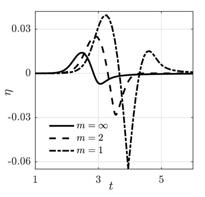
Figure 5: Comparison of the shoreline displacement for identical incident Gaussian waves given by (12) with $a=0.0025$, $b=4.0$ and $x_{0}=1.69$, in a plane beach ($m=\infty$), parabolic bay ($m=2$), and V-shaped bay ($m=1$).

These findings have profound implications not only for coastal engineering in narrow bays or channels, but also for hydraulic engineering. For example, the Vajont dam in Italy is located at the head of narrow V-shaped valley. In 1963, a landslide caused a $\sim 200$ meter high wave that overcame the dam and caused massive destruction to towns downstream. Such events can be modeled using shallow water theory Bosa and Petti (2011), and our results can help explain why the wave was highly amplified in the narrow channel. Understanding the effects of narrow channel bathymetry on wave amplification is crucial for ensuring the safety of communities near bays and dams.

IV Discussion and Conclusions

The current models used for tsunami forecast have primarily been verified against the analytical solutions for sloping bays Synolakis et al. (2008); Kanoglu et al. (2015). With local bathymetry significantly effecting the run-up of tsunami waves, the proposed analytical solution, along with other existing analytical solutions Zahibo et al. (2006); Rybkin et al. (2014); Anderson et al. (2017), allow verification of tsunami models in a more realistic settings of a 2-D bathymetry. Furthermore, 1-D shallow water theory has been shown to have similar inundation predictions to the full 2-D models in the realistic setting of Alaskan fjords, with significantly less computation time Harris et al. (2015b). Incorporating 1-D shallow water theory into large scale tsunami inundation models may significantly reduce computation and forecasting time Harris et al. (2015b); Anderson et al. (2017), potentially saving lives and resources.

When modeling tsunamis generated by near shore earthquakes and submarine landslides, initial conditions must be prescribed directly on the sloping beach. The previous IVP solutions had some limitations to modeling such phenomena because of the linearization of the initial conditions Carrier et al. (2003) or certain implicit assumptions Kanoglu and Synolakis (2006). The presented solution is a further step towards modeling such near-field events, which are the Achilles heel of current tsunami models Kanoglu et al. (2015); Synolakis and Bernard (2006); Kanoglu and Synolakis (2015). The initial conditions associated with submarine landslides are still debated and we refer the interested reader to Løvholt et al. (2015).

On the other hand, earthquakes in the open ocean generate waves that propagate from far off-shore, and then deform over a sloping beach. This problem is modeled as a boundary value problem Kanoglu and Synolakis (2006); Synolakis (1987), though specifying the boundary condition is nontrivial Antuono and Brocchini (2007). Analysis of our solution infers that the zeroth order projection of the initial conditions (i.e. $\Phi_{0}$) is likely adequate for modeling runup of geophysical tsunamis. As the ocean side of the sloping beach is usually far from shore, the wave should behave linearly at this boundary, and zeroth order approximation of the boundary condition could be sufficient. To model water velocities is likely necessary to use the first order projection (i.e. $\Phi_{1}$), however further investigations are necessary. We also would like to emphasize the computational expenses to compute various projections $\Phi_{n}$, $n=0,\dots,10$ according to (11) are negligibly small in comparison to evaluating of integral in (6).

To conclude, in this letter we formulate a new complete solution to the IVP of the cross-sectionally averaged SWE for initial conditions with and without initial velocity. This proposed solution deals with the difficulty associated with the initial conditions given on a curve in the transformed space, an important subtlety not previously acknowledged, and also avoids linearizion of the spatial coordinate in the transformation of the initial conditions. This allows modeling problems with near shore initial conditions, and extends earlier solutions beyond waves with small initial velocities. It also extends the solution from only plane beaches to more complex U-shaped bathymetries. Our proposed solution can be used for analytical verification of tsunami models in realistic 2-D settings, and may potentially allow fast tsunami forecasting in narrow bays and fjords.

*

Appendix A Appendix: Analysis of solution in Kanoglu and Synolakis (2006)

We would like to examine a solution to the non-linear shallow water equation provided in Kanoglu and Synolakis (2006). In particular, we would like to analyze formula (4) in Kanoglu and Synolakis (2006), namely:

$$\psi(\sigma,\lambda)=2\int_{0}^{\infty}\Big{[}\psi(\xi,\lambda_{0})G_{\lambda}+\psi_{\lambda}(\xi,\lambda_{0})G\Big{]}d\xi.$$ (13)

Here, the quantity $G$ is given by

$$G(\xi,\sigma,\bar{\lambda})=\xi\int_{0}^{\infty}{J_{0}}(\omega\xi)J_{0}(\omega\sigma)\sin\big{(}\frac{1}{2}\omega\bar{\lambda}\big{)}d\omega,$$

where $\bar{\lambda}=\lambda-\lambda_{0}$. Note that $\lambda_{0}=\lambda_{0}(\sigma)=-u_{0}(x(\sigma))$. We now show that if $\psi(\sigma,\lambda)$ is given by Eq. (13) then

$$4\sigma\psi_{\lambda\lambda}-(\sigma\psi_{\sigma})_{\sigma}=O(\frac{\partial{\lambda_{0}}}{\partial\sigma})\not=0$$ (14)

which means that (13) is not an exact solution to the shallow water equations in the transformed coordinates, see formula (3) in Kanoglu and Synolakis (2006).

To this end, consider

$$I(\sigma,\lambda)\equiv 2\int_{0}^{\infty}\Big{[}\psi(\xi,\lambda_{0})G_{\lambda}+\psi_{\lambda}(\xi,\lambda_{0})G\Big{]}d\xi.$$

Inserting the expression for $G$ (the Green’s function) in the integral, one has

$$I =\int_{0}^{\infty}\psi(\xi,\lambda_{0})\Big{[}\xi\int_{0}^{\infty}\omega{J_{0}}(\omega\xi)J_{0}(\omega\sigma)\cos\big{(}\frac{1}{2}\omega\bar{\lambda}\big{)}d\omega\Big{]}d\xi$$

$$+2\int_{0}^{\infty}\psi_{\lambda}(\xi,\lambda_{0})\Big{[}\xi\int_{0}^{\infty}{J_{0}}(\omega\xi)J_{0}(\omega\sigma)\sin\big{(}\frac{1}{2}\omega\bar{\lambda}\big{)}d\omega\Big{]}d\xi.$$

Interchanging the order of integration yields

$$I =\int_{0}^{\infty}\omega{J_{0}}(\omega\sigma)\cos\big{(}\frac{1}{2}\omega\bar{\lambda}\big{)}\int_{0}^{\infty}\xi{J_{0}}(\omega\xi)\psi(\xi,\lambda_{0})d\xi d\omega$$

$$+2\int_{0}^{\infty}{J_{0}}(\omega\sigma)\sin\big{(}\frac{1}{2}\omega\bar{\lambda}\big{)}\int_{0}^{\infty}\xi{J_{0}}(\omega\xi)\psi_{\lambda}(\xi,\lambda_{0})d\omega d\xi$$

$$=\int_{0}^{\infty}\omega{J_{0}}(\omega\sigma)\cos\big{(}\frac{1}{2}\omega\bar{\lambda}\big{)}\overline{P}(\omega)d\omega+2\int_{0}^{\infty}{J_{0}}(\omega\sigma)\sin\big{(}\frac{1}{2}\omega\bar{\lambda}\big{)}\overline{F}(\omega)d\omega$$

$$=I_{1}+I_{2},$$

where

$$\overline{P}(\omega)=\int_{0}^{\infty}\sigma{J_{0}}(\omega\sigma)\psi(\sigma,\lambda_{0})d\sigma,~{}~{}~{}~{}~{}~{}~{}~{}\overline{F}(\omega)=\int_{0}^{\infty}\sigma{J_{0}}(\omega\sigma)\psi_{\lambda}(\sigma,\lambda_{0})d\sigma$$

are the Fourier-Hankel transforms of $\psi(\sigma,\lambda_{0})$ and $\psi_{\lambda}(\sigma,\lambda_{0})$.

We now substitute $I$ in the left hand side of equation (14). Since (14) is linear and $\overline{P}(\omega)$ and $\overline{F}(\omega)$ are independent, it is enough to consider only

$$I_{1}(\sigma,\lambda)=\int_{0}^{\infty}\omega{J_{0}}(\omega\sigma)\cos(\frac{1}{2}\omega\bar{\lambda})\overline{P}(\omega)d\omega.$$

By a straightforward computation we obtain

$$4\sigma\frac{\partial^{2}}{\partial\lambda^{2}}{I_{1}}-\frac{\partial}{\partial\sigma}\Big{(}\sigma\frac{\partial}{\partial\sigma}{I_{1}}\Big{)}=\int_{0}^{\infty}\omega\Delta_{1}(\sigma,\lambda,\omega)\overline{P}(\omega)d\omega,$$

where

$$\Delta_{1}(\sigma,\lambda,\omega)$$

$$=\sigma(-\omega^{2}){J_{0}}(\omega\sigma)\cos(\frac{1}{2}\omega\bar{\lambda})-\frac{\partial}{\partial\sigma}\Big{(}\sigma\frac{\partial}{\partial\sigma}\big{(}{J_{0}}(\omega\sigma)\cos(\frac{1}{2}\omega\bar{\lambda})\big{)}\Big{)}$$

$$=-\frac{\omega}{2}\Big{(}2\sigma\frac{\partial{J_{0}(\omega\sigma)}}{\partial\sigma}+{J_{0}}(\omega\sigma)\Big{)}\sin(\frac{1}{2}\omega\bar{\lambda})\frac{\partial{\lambda_{0}}}{\partial\sigma}$$

$$+\frac{\omega}{2}\sigma{J_{0}}(\omega\sigma)\frac{\partial}{\partial\sigma}\Big{(}\sin(\frac{1}{2}\omega\bar{\lambda})\frac{\partial\lambda_{0}}{\partial\sigma}\Big{)}$$

$$=O(\frac{\partial{\lambda_{0}}}{\partial\sigma}).$$

Consequently,

$$4\sigma\frac{\partial^{2}}{\partial\lambda^{2}}{I}-\frac{\partial}{\partial\sigma}\Big{(}\sigma\frac{\partial}{\partial\sigma}{I}\Big{)}=O(\frac{\partial{\lambda_{0}}}{\partial\sigma})$$

and no better. This implies that formula (13) does not solve the wave equation (14), but provides an approximation to the solution up to order at least ${\partial{\lambda_{0}}}/{\partial\sigma}$ (or equivalently ${\partial{u_{0}}}/{\partial\sigma}$). We note that if the initial velocity $u_{0}=0$ then ${{\lambda_{0}=0}}$ and the error term vanishes. I.e. $I\left(\sigma,\lambda\right)$ is then indeed an exact solution (but not in general).