Multiple Explanations for the Single Transit of KIC 5951458 Based on Radial Velocity Measurements Extracted with a Novel Matched-template Technique

Abstract

Planetary systems that show single-transit events are a critical pathway to increasing the yield of long-period exoplanets from transit surveys. From the primary Kepler mission, KIC 5951458 b (Kepler-456b) was thought to be a single-transit giant planet with an orbital period of 1310 days. However, radial velocity (RV) observations of KIC 5951458 from the HIRES instrument on the Keck telescope suggest that the system is far more complicated. To extract precise RVs for this $V\approx 13$ star, we develop a novel matched-template technique that takes advantage of a broad library of template spectra acquired with HIRES. We validate this technique and measure its noise floor to be 4–8 m s^-1 (in addition to internal RV error) for most stars that would be targeted for precision RVs. For KIC 5951458, we detect a long-term RV trend that suggests the existence of a stellar companion with an orbital period greater than a few thousand days. We also detect an additional signal in the RVs that is possibly caused by a planetary or brown dwarf companion with mass in the range of 0.6–82 $M_{\rm Jup}$ and orbital period below a few thousand days. Curiously, from just the data on hand, it is not possible to determine which object caused the single “transit” event. We demonstrate how a modest set of RVs allows us to update the properties of this unusual system and predict the optimal timing for future observations.

1 Introduction

The vast majority of known transiting exoplanets whip around their host stars on orbits of 10 days or less. The detection of transiting exoplanets with short orbital periods results from the twofold bias of the transit method. First, the geometric probability of observing an exoplanet transit scales inversely with the physical separation between the planet and the star. Second, the finite observational baseline reduces the probability of detecting exoplanets that have relatively long orbital periods. Considering both biases, the best means of extending the range of orbital periods of known transiting exoplanets is to observe many stars for as long as possible.

This was the approach of the primary Kepler mission, which achieved a nearly continuous, 4 yr observational baseline for over 150,000 stars (Borucki et al., 2010). This baseline is so far unrivaled among transit surveys, as is the sample of long-period transiting exoplanets identified in the Kepler data set. Long-period exoplanets are more readily discovered through radial velocity (RV) measurements of their host stars. However, the fortuitous alignment that causes a transit also enables analyses that simply cannot be conducted for most RV-detected exoplanets. This means that the long-period sample of transiting exoplanets (e.g., Kawahara & Masuda, 2019) is small, but each one is extraordinarily valuable.

Among these exoplanets is KIC 5951458 b (also known as Kepler-456b), a supposed $\sim$6.6 Earth-radius planet candidate that was only observed to transit once during the Kepler primary mission (Wang et al., 2015; Kawahara & Masuda, 2019). The two previous efforts to characterize this planet candidate measured an orbital period in the range of 1167.6–13721.9 days (Wang et al., 2015) and 1600${}^{+1100}_{-400}$ days (Kawahara & Masuda, 2019). Neither estimate is precise owing to the lack of additional transits. KIC 5951458 b was not categorized as a Kepler object of interest (KOI) by the Kepler pipeline (e.g., Thompson et al., 2018), but subsequent analysis led to its statistical validation (Wang et al., 2015). Statistical validation of exoplanets is a common technique that typically involves ruling out enough of the false-positive scenario parameter space to claim the planetary nature to some probability threshold (e.g., Barclay et al., 2013; Crossfield et al., 2016; Morton et al., 2016). In the case of KIC 5951458 b, the statistical validation process produced a planet probability of 99.8% (Wang et al., 2015). Ideally, validated exoplanets like KIC 5951458 b would also receive sufficient follow-up observation to uniquely measure their mass, which more clearly determines their nature. However, given the ever-growing number of candidates from planet discovery efforts such as Kepler, K2 (Howell et al., 2014), and the Transiting Exoplanet Survey Satellite (TESS; Ricker et al., 2015), statistical validation techniques are becoming increasingly common.

In this work, we explore the validated exoplanet KIC 5951458 b by acquiring a small number of RV observations of its host star. We do not attempt to conduct a full characterization of this system; such an effort will not be possible for many single-transit candidate exoplanets that have been (or will be) discovered by Kepler or TESS. For Kepler single-transit detections, baselines of several years are likely required to cover a full orbit. Additionally, the faintness of typical Kepler host stars severely limits the list of facilities capable of making precise RV measurements. In the case of TESS single-transit detections, time baselines are shorter and host stars are brighter (e.g., Dalba et al., 2020; Eisner et al., 2020; Gill et al., 2020), and the number of detections is expected to be much higher than for Kepler (e.g., Villanueva et al., 2019). As a result, follow-up resources must be used strategically to maximize the science return from single-transit detections. For KIC 5951458, we collect only a modest set of RVs that we then combine with archival data to identify inaccuracies in the currently published properties of KIC 5951458 b. We then demonstrate how a careful consideration of possible scenarios for the nature of the KIC 5951458 system enables informed predictions for future observations.

In Section 2, we identify and process archival observations of KIC 5951458, which include photometry from all quarters of the Kepler primary mission and adaptive optics (AO) imaging. In Sections 3 and 4, we present RV observations of KIC 5951458 from the High Resolution Echelle Spectrometer (HIRES) at the 10 m Keck I telescope. We describe a new method of extracting precision RV measurements that involves matching KIC 5951458 to a star in the HIRES spectral library that already has a spectral template. We validate this method and demonstrate its benefit for faint host stars like those observed by Kepler. In Section 5, we employ the rejection sampling package The Joker (Price-Whelan et al., 2017) to model the RVs. We find that KIC 5951458 likely hosts both a stellar companion and a giant planetary or brown dwarf companion, but it is not clear which one caused the occultation event observed by Kepler. In Section 6, we discuss the various scenarios for the nature of the KIC 5951458 system in the context of other known exoplanets and binary star systems. We also place our efforts for this system in the context of similar ongoing research, mostly related to the TESS mission. Finally, in section 7, we summarize our findings for the remarkable KIC 5951458 system.

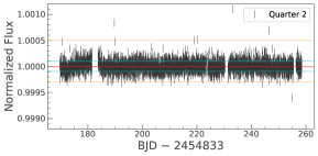
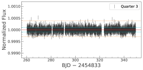
Figure 1: Long-cadence Kepler PDCSAP light curves of KIC 5951458 from the entire Kepler primary mission. The red lines denote the median of each light curve, and the blue and orange lines are plotted at percentiles that approximate the $\pm 1\sigma$ and $\pm 3\sigma$ fluxes, respectively. The single occultation that led to the original validation of KIC 5951458 b is clearly visible in Quarter 4. There are no statistically appreciable counterparts to this event (i.e., transits or eclipses).

2 Archival Data

The combination of high-precision photometry and AO imaging led to the initial validation of KIC 5951458 b (Wang et al., 2015). Here, we present these archival data because they provide critical context to the reevaluation of the properties of the KIC 5951458 system.

2.1 Kepler Photometry

The Kepler spacecraft observed KIC 5951458 in each quarter of the primary Kepler mission (Figure 1). We acquire all Kepler photometry of KIC 5951458 from the Milkuski Archive for Space Telescopes (MAST) using the Lightkurve package (Lightkurve Collaboration et al., 2018). We use the pre-search data conditioning photometry (PDCSAP) from Data Release 25. This release, which uses version 9.3 of the Science Operations Center pipeline, benefits from an accurate determination of the stellar scene and crowding metrics that mitigates errors from so-called “phantom stars” (Dalba et al., 2017) and that leads to higher photometric precision in general (Twicken et al., 2016). We remove long-term variability from each quarter’s PDCSAP light curve using a Savitzky–Golay filter (Savitzky & Golay, 1964). Figure 1 shows the resulting light curves of KIC 5951458. Each panel presents a single quarter, with horizontal lines denoting the following percentiles of the photometry: {0.1, 15.9, 50, 84.1, 99.9}. Visual inspection readily identifies the single occultation event in Quarter 4. Besides this occultation, there are no other statistically significant dimming events (i.e., transits or eclipses) in the light curves.

Figure 2 provides a detailed look at the single occultation from Quarter 4. The occultation depth ($\sim$0.1%) is sufficiently small to suggest that the occulter is planetary in size, but the long ingress and egress durations relative to the occultation duration (i.e., second to third contact) suggest that it was possibly grazing. Indeed, a recent effort to characterize this single occultation inferred an impact parameter of 0.94${}^{+0.01}_{-0.02}$ (Kawahara & Masuda, 2019). This leads to a degeneracy between parameters that prevents the accurate estimation of the size of the occulting object.

Figure 2: Single occultation event for KIC 5951458 observed by Kepler during Quarter 4 of the primary mission. The depth is consistent with a planetary transit, but the shape and duration indicate that it could be a grazing event by a larger body.

The duration of the single occultation event in Quarter 4 is approximately 12.3 hr. This is sufficiently long to suggest that the occulter has a long orbital period relative to the majority of known transiting exoplanets, especially considering that the occultation is likely grazing. Alternatively, the large (albeit imprecise) radius of KIC 5951458 (see Table 1) causes a longer-duration occultation than a smaller star for a planet with a fixed orbital period. Based on analysis of the single occultation, Wang et al. (2015) estimated that the orbital period of KIC 5951458 b is $1320.10^{+12401.80}_{-152.50}$ days. Similarly, Kawahara & Masuda (2019) estimated that the orbital period is $1600^{+1100}_{-400}$ days.

Table 1: Properties of the KIC 5951458 System

Property	Value
Alias	Kepler-456 (b)
R.A. (J2000)	19h 15m 57.979s
Decl. (J2000)	+41d 13m 22.909s
Kepler magnitude	12.713
Spectral type	F5V
Distance (pc)	$743\pm 12$
	HIRES spectrum	Kawahara & Masuda (2019)
$T_{\rm eff}$ (K)	$5930\pm 110$	$5993^{+99}_{-88}$
$R_{\star}$ ($R_{\sun}$)	$1.34\pm 0.18$	$1.81^{+0.03}_{-0.04}$
$[$Fe/H$]$ (dex)	$-0.09\pm 0.09$	$-0.05\pm 0.09$
$M_{\star}$ ($M_{\sun}$)	$1.16\pm 0.04$	$1.20^{+0.05}_{-0.03}$
log $g$ (cgs)	$4.10\pm 0.10$	$4.00\pm 0.02$
$V\sin{i}$ (km s-1)	$3.6\pm 1.0$	$\cdots$
Age (Gyr)	$\cdots$	$4.5^{+1.0}_{-0.4}$

2.1.1 A Lower Limit on Orbital Period

We do not attempt to make a new orbital period measurement from the Quarter 4 occultation event. Instead, we take advantage of the substantial baseline of the Kepler photometry along with the clear nondetection of additional events to estimate a lower limit on this orbital period that does not rely on the event duration. In the simplest case, assuming that an additional occultation event could not have occurred at any time during the primary Kepler mission (such as in a data gap), the shortest possible orbital period would be the time between the end of Quarter 17 and the occultation event in Quarter 4: 1168 days.

However, we also take a more conservative approach to estimate this lower limit. For orbital periods between 1 and 1168 days, incremented by 1 day, we inject identical occultation events into the Kepler light curves. The conjunction time for each period is fixed to the observed occultation timing. If less than half of an occultation occurs during a data gap, we expect that event to have been detected since the photometric precision in each quarter’s light curve is well below the occultation depth. Following this procedure, candidate orbital periods will be those that only yield one detection (i.e., the actual occultation in Quarter 4). We find 56 candidate orbital periods below 1168 days, the shortest of which is 609 days. In later analyses (Section 5.1), we will treat this value as the shortest possible orbital period of the object that caused the Quarter 4 occultation.

2.2 NIRC2 Adaptive Optics Imaging

AO imaging of KIC 5951458 was conducted using the NIRC2 instrument (Wizinowich et al., 2000) on the Keck II telescope (Wang et al., 2015). Images were taken in the $K_{s}$ band to search for stellar companions that may have contaminated the flux in the Kepler apertures or that may indicate that the occultation signal is a false-positive. No stellar companions were identified for KIC 5951458. Instead, limits were placed on the magnitude difference between a potential undetected stellar companion and KIC 5951458 (Figure 3). The detection limits are five times the standard deviation of the flux above the median in concentric annuli at the angular separations shown.

Figure 3: Limits on the magnitude of undetected stellar companions to KIC 5951458 based on NIRC2 AO imaging (Wang et al., 2015). The detection limits are five times the standard deviation of the flux above the median in concentric annuli at the angular separations shown. The projected physical separation is simply the product of the angular separation and known distance to KIC 5951458.

The non-detection of additional stellar components in the KIC 5951458 AO images contributed to the confidence that the observed occultation was not some sort of false-positive scenario. However, this observation does not clearly distinguish between the scenarios of a planet transit or a grazing eclipse of a stellar companion. The distance between KIC 5951458 and the solar system (Table 1) limits the inner edge of the AO detection limit to $\sim 70$ au. Stellar or planetary companions could certainly orbit the host star well within this separation and could have the proper inclination to cause either a transit or an eclipse. Furthermore, there is also a small possibility that the AO observations occurred near the time of inferior or superior conjunction of the stellar companion.

3 Spectroscopic Observations

Despite the apparent grazing nature of the occultation event, the degeneracy between planetary radius and impact parameter, the weak constraint on orbital period, and the limited AO imaging, the observations of KIC 5951458 b were sufficient to validate its planetary nature at a confidence of 99.8% (Wang et al., 2015). In the following sections, we describe efforts to extend the analysis of KIC 5951458 to include spectroscopic characterization and Doppler monitoring with the goal of measuring the mass and determining the planetary nature of KIC 5951458 b.

3.1 Spectroscopic Properties

We began this process by acquiring an iodine-free spectrum of KIC 5951458 with HIRES (Vogt et al., 1994) on the Keck I telescope. The signal-to-noise ratio (S/N) of this spectrum is $\sim$40, which is sufficient to rule out the presence of a second set of spectral lines and to conduct a basic spectroscopic analysis of KIC 5951458. We use SpecMatch-Emp, an empirical spectrum matching technique (Yee et al., 2017), to infer the stellar radius ($R_{\star}$), stellar effective temperature ($T_{\rm eff}$), and iron abundance ($\rm[Fe/H]$) of KIC 5951458. SpecMatch-Emp does not compute stellar surface gravity ($\log{g}$), mass ($M_{\star}$), or projected rotational velocity ($V\sin{i}$). Instead, we employ the SpecMatch technique (Petigura, 2015; Petigura et al., 2017) to calculate these properties. SpecMatch interpolates a grid of model stellar spectra and is especially suited to low-S/N, iodine-free spectra acquired with HIRES. The resulting spectroscopic properties of KIC 5951458 are listed in Table 1.

The properties of KIC 5951458 place it in a region of parameter space near the edge of SpecMatch’s applicability. Therefore, we also list the spectroscopic properties of KIC 5951458 from Kawahara & Masuda (2019) in Table 1. Kawahara & Masuda (2019) processed a spectrum acquired with the Large Sky Area Multi-Object Fiber Spectroscopic Telescope (Cui et al., 2012; Luo et al., 2015) using SpecMatch-Emp and isochrone modeling. This characterization included parallax measurements from the Gaia mission (Bailer-Jones et al., 2018; Gaia Collaboration et al., 2018). Since the applicability of SpecMatch to KIC 5951458 is questionable, we hereafter adopt all stellar properties of KIC 5951458 from Kawahara & Masuda (2019) except for $V\sin{i}$, which was not reported from that analysis.

4 Doppler Monitoring and the Matched-template Technique

To explore possible false-positive scenarios for the KIC 5951458 b occultation event, we conducted a Doppler monitoring campaign with HIRES on the Keck I telescope. We acquired six high-resolution ($R\approx 60,000$) spectra of KIC 5951458. A heated iodine cell in the light path in front of the slit enables precise wavelength calibration of each RV measurement. The observed spectrum, which is the combination of the stellar and the gaseous iodine spectra, is then forward modeled following standard procedures of the California Planet Search (e.g., Howard et al., 2010; Howard & Fulton, 2016).

Iodine-calibrated RV measurements have a long history of producing precise velocities (Marcy & Butler, 1992) but one of the primary limitations of the technique is the need to acquire a high-S/N, iodine-free spectrum of the star. This “template” observation is deconvolved from the instrumental point spread function (PSF) that is derived from bracketing observations of rapidly rotating B stars (taken with the iodine cell) to construct a “deconvolved stellar spectral template” (DSST). This deconvolution requires the template to be high-S/N, ideally near 200 per pixel. During the forward modeling process, the DSST is multiplied by an ideal iodine absorption spectrum as measured with a Fourier transform spectrograph and then convolved with the PSF derived for each observation. Since HIRES is slit-fed, the PSF is highly dependent on the precise illumination pattern of the slit, which is affected by changes in seeing and guiding. The variable PSF requires a complex model with 12 free parameters that is capable of modeling tiny asymmetries in the PSF. The large number of free parameters combined with noise amplification in the deconvolution process drives the need for high S/N ($\sim$200) for high RV precision ($\sim$1 m s^-1). This makes it impractically expensive to observe faint targets like KIC 5951458, which would require an hour-long exposure to reach an S/N of only $\sim$100.

Fulton et al. (2015) developed a technique to utilize model stellar spectra in place of the DSST and showed that RV precision of $\sim$5–15 m s^-1 precision could be achieved without observing a template of the target star. In addition, the noise-free (model) template spectrum allows for much lower S/N for each RV observation. However, this technique is limited to the relatively narrow regime of FGK main-sequence dwarf stars, where the Coelho et al. (2005) models are sufficiently accurate.

Yee et al. (2017) utilized decades of archival HIRES data to construct a library of high-quality template spectra and developed a technique to match these spectra to an observed, low-S/N, iodine-free observation to extract precise stellar parameters (SpecMatch-Emp). In this work, we use this library and spectral matching technique to identify a spectrum in the California Planet Search archive that can be substituted for the DSST. For any star without a DSST, we identify the member of the library with the most similar spectrum as quantified by the absolute $\chi^{2}$ statistic. Some of the stars in the Yee et al. (2017) template library were not observed with bracketing B stars and therefore cannot be used to derive DSSTs. Figure 4 plots the SpecMatch-Emp library on a spectroscopic Hertzprung-Russell (HR) diagram and shows the distribution of library stars with and without DSSTs. Fortunately, 323 of the 404 library stars were observed appropriately and have associated DSSTs in the HIRES database. The stars have effective temperatures spanning from $\sim$6500 K to $\sim$3000 K and $\log{g}$ from $\sim$5 to 2.5 dex, making this technique possible for the majority of main-sequence and subgiant stars amenable to precision RVs.

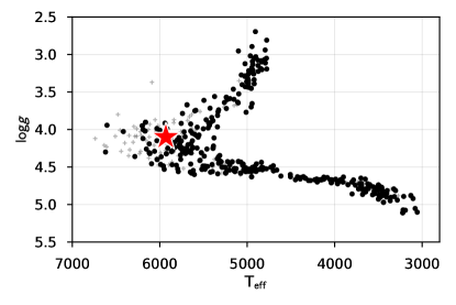
Figure 4: Spectroscopic H-R diagram of the SpecMatch-Emp library. KIC 5951458 is represented by the red star. Stars with DSSTs are plotted as black circles, and library stars without DSSTs are plotted as gray plus signs. Our DSSTs span F to M dwarfs, as well as the majority of the subgiant branch.

4.1 Validation of the Matched-template Technique

We validate the matched-template technique by applying it to the HIRES template library. Since each star in the library has its own template, its RVs can be used as a “ground truth” in the comparison with RVs produced via the matched-template technique. This comparison can also be conducted as a function of stellar properties to additionally explore the sensitivity and limitations of the technique.

We begin by identifying the subset of the 323 stars in the DSST library that are appropriate for this test. We require that stars have at least three iodine-in spectral observations. This criterion removes nine stars. We also require that each star can be suitably matched with another in the library. This criterion removes 67 stars, most of which reside in relatively isolated regions of parameter space. This leaves 247 stars for the test of the matched-template technique. The range of stellar properties of these stars is displayed in Figure 5.

Figure 5: Stellar properties of the 247 stars in the HIRES DSST library on which the matched-template technique is tested and the corresponding rms of the RV residuals (Equation 1). These panels show that the matched-template technique can be applied to a wide variety of stars. However, we identify groups of stars of various properties that have slightly different distributions of rms values (shown in Figure 7). We separate the groups with dotted lines, the values of which are given in Table 2.

For each of the 247 stars, we select up to the 100 spectra with the highest S/N. We process each of these spectra twice: once using the template of the star itself, and once using the best-match star’s template. The best-match star is chosen to be the one with the most similar spectrum, as quantified by the absolute $\chi^{2}$ statistic. Hereafter, we will use the subscripts “self” and “match” to refer to RV data products produced using a star’s own template and its best-match star’s template, respectively. For each star, we calculate the rms of the residuals between the two RV time series as

$${\rm rms}=\sqrt{\frac{\sum_{i=1}^{n}[v_{\rm r,match}(t_{i})-v_{\rm r,self}(t_{i})]^{2}}{n}}$$ (1)

where $v_{\rm r}$ is the stellar RV, $t$ is time, and $n$ is the total number of RV observations for the $i$th star. The median number of RVs for each star used in the calculation of the rms is 26, and the mean number of RVs is 37.

Figure 6 shows the distribution of rms values of the RV residuals for all 247 stars. The logarithms of the rms values form a somewhat normal distribution that is skewed toward higher values. The median of this distribution is 4.6 m s^-1, which serves as a first-order estimate of the noise floor of the matched-template method. On average, the rms of the residuals between the $v_{\rm r,match}$ and $v_{\rm r,self}$ time series is larger than the median uncertainty on $v_{\rm r,self}$. We therefore cannot neglect the error that is introduced by the matched-template analysis.

Figure 6: Distribution of rms values of the RV residuals (Equation 1) for the 247 stars tested with the matched-template method. The various statistics provided for this distribution serve as a general assessment of the precision of the matched-template method.

We consider how the method affects the uncertainty of the derived RV measurements as a function of stellar properties. In Figure 5, the rms of the RV residuals is plotted against $T_{\rm eff}$, $R_{\star}$, $\log{g}$, and $V\sin{i}$. The range of the stellar properties spanned in this figure shows that the matched-template method can be applied to many different types of stars. However, different types of stars produce slightly different distributions of rms values (as separated by dotted lines in Figure 5).

For each of the four stellar properties we consider, we divide the stars into two groups. The locations of these divisions are chosen manually and are meant to separate groups of stars with similar properties and also different distributions of rms values. The values of the divisions in stellar properties are listed in Table 2. The resulting distributions of the rms of the RV residuals are shown in Figure 7. In general, these distributions are unimodal but have tails to larger values. The only distributions that are not unimodal (i.e., $T_{\rm eff}\leq 4400$ K and $V\sin{i}>5.0$ km s^-1) contain substantially fewer stars than the others. This demonstrates that for cool stars, or those with relatively high rotation velocity, the matched-template method will have limited accuracy owing to the limited sample of stars in the HIRES template library. For all other distributions, Figure 7 identifies the mean, 50th percentile (i.e., median), and 84th percentile of the rms of the RV residual values. These values are key to understanding how the matched-template method inflates the RV uncertainty.

Table 2 contains the statistics describing the distributions in Figure 7 and is meant to be a “look-up table.” For a given star—with known $T_{\rm eff}$, $R_{\star}$, $\log{g}$, and $V\sin{i}$—four estimates of the rms of the RV residuals for similar stars can be identified (one for each stellar property). The estimates can each be the mean, median, or 84th percentile, the choice of which depends on the particular application of the matched-template method and the error tolerance. Those four estimates of rms can then be combined (e.g., minimum, maximum, median, etc.) to yield a final error values to be added (in quadrature) to the RV internal errors. For example, for a solar analog star, Table 2 yields median values of 4.6 m s^-1 (for $T_{\rm eff}$), 4.6 m s^-1 (for $R_{\star}$), 4.6 m s^-1 (for $\log{g}$), and 4.7 m s^-1 (for $V\sin{i}$), the average of which is 4.6 m s^-1. Based on the needs of the analysis, more or less conservative approaches may be justified, and the values listed in Table 2 allow for those.

Table 2: Error Incurred by the Matched-template Technique as a Function of Stellar Properties

	Statistics Describing rms of RV Residual Distribution (m s-1)
Stellar Properties	Mean	50th Percentile	84th Percentile
Effective temperature (K)
$T_{\rm eff}\leq 4400$	5.2	4.0	8.6
$T_{\rm eff}>4400$	6.5	4.6	7.8
Radius ($R_{\sun}$)
$R_{\star}\leq 3.5$	6.2	4.6	7.8
$R_{\star}>3.5$	6.5	4.2	8.5
Surface gravity (cgs)
log $g\leq 3.6$	6.1	4.5	7.9
log $g>3.6$	6.3	4.6	8.0
Rotational velocity (km s-1)
$V\sin{i}\leq 5.0$	5.9	4.7	14.4
$V\sin{i}>5.0$	18.9	7.8	19.5

Figure 7: Distributions of rms of RV residuals for each group in each of four stellar parameters. The divisions listed here are represented as the dotted lines in Figure 5. In general, these distributions are unimodal with tails to longer values. The only distributions that are not also have relatively few stars. The values of the orange vertical lines shown here are listed in Table 2 and are useful for determining how to inflate the internal error for RVs produced with the matched-template method.

For most stars that would be subject to precise RV measurements, the matched-template method demonstrates the ability to surpass the $\sim$10 m s^-1 noise floor of the synthetic template technique (Fulton et al., 2015) by nearly a factor of two. For faint stars for which acquiring a high-S/N template is infeasible, assuming that there is a suitable best-match star in the HIRES DSST library, the matched-template technique is preferable. Furthermore, the method is also useful for exploring the RV signals of bright stars prior to the acquisition of a template spectrum. It is typical for several iodine spectra to be acquired prior to a template in order to establish a time baseline for the star of interest. The matched-template method enables a first-order assessment of the RVs associated with those iodine-in spectra that aids in planning and has the potential to save observing time.

4.2 Application of the Matched-template Technique to KIC 5951458

We processed the RV observations of KIC 5951458 from Keck-HIRES with the matched-template technique using the DSST for HD 22484. Table 3 lists the properties of HD 22484 inferred from SpecMatch using its high-S/N iodine-free template spectrum. All properties between the two stars are consistent to within the $1\sigma$ uncertainties except stellar radius.

Table 3: Spectroscopic Properties of HD 22484, the Best Match to KIC 5951458

Property	HD 22484
Spectral type	F9IV-V
$T_{\rm eff}$ (K)	$5964\pm 100$
$R_{\star}$ ($R_{\sun}$)	$1.66\pm 0.04$
$[$Fe/H$]$ (dex)	$-0.01\pm 0.06$
$M_{\star}$ ($M_{\sun}$)	$1.13\pm 0.07$
log $g$ (cgs)	$4.07\pm 0.10$
$V\sin{i}$ (km s-1)	$3.29\pm 1.0$

The Keck-HIRES RVs resulting from the matched-template analysis of KIC 5951458 are listed in Table 4 and are hereafter assigned to the symbol $v_{\rm r}$. The internal errors on $v_{\rm r}$ are $\sim$3 m s^-1. We follow the procedure outlined in Section 4.1 to determine the amount by which we must increase these errors to account for the matched-template method. Based on the properties of KIC 5951458 in Table 1, we identify rms of the RV residuals values of 6.5 m s^-1 (for $T_{\rm eff}$), 6.2 m s^-1 (for $R_{\star}$), 6.3 m s^-1 (for $\log{g}$), and 5.9 m s^-1 (for $V\sin{i}$) from Table 2. We have chosen to use the mean values of the rms distributions as a conservative trade-off between the 50th and 84th percentiles. The average of these four values is 6.2 m s^-1, which we add in quadrature to the internal RV errors. The resulting uncertainty in $v_{\rm r}$ is denoted as $\sigma_{v_{\rm r}}$ and is listed in Table 4.

Table 4: Keck-HIRES RV Measurements for KIC 5951458

Time	Telluric RV $v_{\rm t}$	$\sigma_{v_{\rm t}}$	Precise RV $v_{\rm r}$	$\sigma_{v_{\rm r}}$	$S_{\rm HK}$
(BJDTDB)	(km s-1)	(km s-1)	(m s-1)	(m s-1)
2458386.74225	$-22.39$	0.10	$1463.4$	6.8	$0.130\pm 0.001$
2458393.88630	$-22.47$	0.10	$1400.1$	7.0	$0.133\pm 0.001$
2458622.98313	$-24.09$	0.10	$-178.6$	6.8	$0.136\pm 0.001$
2458659.08536	$-24.62$	0.10	$-447.5$	6.8	$0.130\pm 0.001$
2458723.98153	$-25.13$	0.10	$-910.5$	6.7	$0.124\pm 0.001$
2458780.81064	$-25.46$	0.10	$-1324.8$	6.7	$0.126\pm 0.001$

A corresponding $S_{\rm HK}$ activity indicator is listed with each RV measurement. The HIRES spectra include the Ca II H and K lines, which enable the calculation of the $S_{\rm HK}$ activity indicators (Wright et al., 2004; Isaacson & Fischer, 2010). We find that the Pearson correlation coefficient between the RVs and $S_{\rm HK}$ values is 0.54, and the corresponding two-tailed $p$-value is 0.27.

We also list the low-precision, telluric-calibrated RVs for KIC 5951458 in Table 4. These measurements and their corresponding uncertainties are given the symbols $v_{\rm t}$ and $\sigma_{v_{\rm t}}$, respectively. These RVs were calculated following the methodology of Chubak et al. (2012). They are absolute in that they share a common zero-point with other studies (Latham et al., 2002; Nidever et al., 2002). The telluric RVs of KIC 5951458 are necessary for analysis conducted in Section 5.2.

Upon first glance, the RV time series of KIC 5951458 displays a trend on the order of several kilometers per second (Figure 8). These RV measurements are extremely linear over the 394-day baseline; the Pearson correlation coefficient between time and RV is $-$0.99994. This trend is indicative of a massive companion on a long-period orbit. When combined with the shape and duration of the occultation event in the Kepler photometry, the RVs may suggest that KIC 5951458 b is a misidentified grazing, eclipsing binary. However, a closer inspection of the RVs uncovers an additional (potentially Keplerian) signal on top of the large trend. Could there be a planet in this binary system that indeed caused the occultation event observed by Kepler?

Figure 8: Top: Keck-HIRES RV measurements of KIC 5951458 extracted using the matched-template analysis. Bottom: RV measurements after removing the trend with a linear regression. Note the difference in scale between the two panels. The errors shown here and used in this analysis include the uncertainty incurred by the matched-template technique (see Section 4.1).

5 Rejection Sampling Analysis

With only six RV observations, a single occultation event, and a nondetection in the AO imaging, we cannot uniquely determine the properties and architecture of the KIC 5951458 system. However, we can explore a wide range of stellar, substellar, and planetary solutions that are consistent with these data to make useful inferences and predictions.

We model the RV observations with the The Joker (Price-Whelan et al., 2017). The Joker is a Monte Carlo sampler that specifically models RV observations of two-body systems. This package employs a specific case of rejection sampling whereby the prior probability distribution functions (PDFs) of the model parameters are densely sampled and their likelihood is used as the rejection scalar. The Joker is able to sample the posterior PDF of the model parameters despite the complex nature of the likelihood function and despite sparse or low-precision data.

By construction, the choice of prior PDFs for the model parameters is critical to the rejection sampling analysis. In all cases, we employ the default priors of The Joker (Price-Whelan et al., 2017). For the companion orbital period ($P$), the prior PDF is uniform in the natural log of $P$ between some minimum ($P_{\rm min}$) and maximum ($P_{\rm max}$) values. The values of $P_{\rm min}$ and $P_{\rm max}$ are chosen on a case-by-case basis as described below. For the companion orbital eccentricity ($e$), the prior PDF is a beta distribution with shape parameters $s_{1}=0.867$ and $s_{2}=3.03$. This particular beta distribution is empirically motivated by observations of RV exoplanets (Kipping, 2013). For the argument ($\omega$) and phase ($\phi_{p}$) of periastron, the prior PDFs are uniform over the domain (0, 2$\pi$). The semiamplitude ($K$) and the systemic velocity ($\gamma$) vary linearly with the RV and are treated differently than the previous four. The prior PDFs for $K$ and $\gamma$ are assumed to be broad Gaussian functions, such that they are essentially uniform over the range of interest (Price-Whelan et al., 2017). Lastly, for all cases we hold the RV jitter fixed at 0 m s^-1.

In the following sections, we divide our analyses based on the different signals in the RV data. First, in Section 5.1, we use The Joker to remove the long-term RV trend and characterize the potential planetary signal (Figure 8, bottom panel). The plausibility of a planetary culprit of the occultation event is also considered. Then, in Section 5.2, we use The Joker to characterize the long-term RV trend (Figure 8, top panel), ignoring the planetary signal. We also consider the possibility that the Kepler occultation is actually the result of an eclipsing binary system. Finally, in Section 5.3, we synthesize the results of both rejection sampling analyses.

5.1 The Potential Planetary Signal

To investigate the potential planetary signal in the RV measurements of KIC 5951458 (Figure 8, bottom panel), we use The Joker with an additional parameter for the first-order acceleration of the companion ($\dot{\gamma}$). We account for the trend in the data using the median value of the posterior PDF for $\dot{\gamma}$. In this application of The Joker, the prior on orbital period is bounded by $P_{\rm min}=10$ days and $P_{\rm max}=100,000$ days. These value are chosen by iterating over increasingly wider domains in $P$ until the shape of the posterior PDF shows no appreciable changes. We use The Joker to sample the prior PDFs $2^{21}$ times. Of these, 38,466 samples of the posterior PDFs survive.

The marginal posterior PDFs from all solutions for $P$ and $K$ are shown in Figure 9. The PDF for $K$ is unimodal, although non-Gaussian, and 93% of samples are below 100 m s^-1. The PDF for $P$ is more complicated, with multiple regions of posterior probability for orbital periods between 10 and 100 days along with a wide, non-Gaussian distribution peaked at $\sim$430 days. Almost no solutions have $P>10,000$ days.

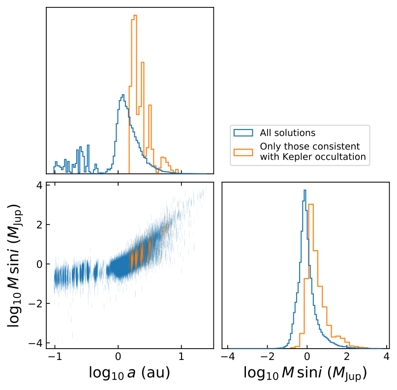
Figure 9: Left panels: marginal posterior PDFs for orbital period ($P$) and RV semiamplitude ($K$) from the rejection sampling of the potential planetary signal. The dashed line shows the 5th percentile in orbital period for solutions that are consistent with the Kepler occultation (orange). Right panels: marginal posterior PDFs for the derived parameters companion minimum mass ($M\sin{i}$) and orbital semi-major axis ($a$). Both groups of panels show the posteriors for all solutions (blue), as well as the subset consistent with the Kepler occultation (orange). For the latter, 95% of solutions have $M\sin{i}=0.6-82\;M_{\rm Jup}$ and $P>687$ days, suggesting that the companion would likely be a long-period giant planet or brown dwarf.

We also derive and display in Figure 9 the posterior PDFs from all solutions for orbital semi-major axis ($a$) and the companion minimum mass ($M\sin{i}$). In doing so, we solve for $M\sin{i}$ numerically and do not assume that the companion mass is negligible compared to the host mass. The PDF for $a$ mirrors that for $P$. The $M\sin{i}$ posterior PDF peaks at 0.75 $M_{\rm Jup}$ and 95% of samples are in the range of 0.2–20 $M_{\rm Jup}$. This distribution suggests that if this RV signal is caused by a companion, then that companion is likely a giant planet or a brown dwarf.

Could this potential giant planet or brown dwarf be the cause of the occultation observed by Kepler? The depth of the occultation is readily consistent with a grazing transit of a 1 $R_{\rm Jup}$ object. However, we address this question in more detail by considering the subset of the rejection sampling solutions that are consistent with the Kepler occultation. For each solution, we determine the time of inferior conjunction (in BJD_TDB) in the vicinity of the Kepler occultation. We calculate the true anomaly ($f$) during transit

$$f=\frac{\pi}{2}-\omega\;,$$ (2)

the corresponding eccentric anomaly ($E$; Murray & Dermott, 1999, p. 33)

$$E=2\;\mathrm{tan}^{-1}\left[\sqrt{\frac{1-e}{1+e}}\;\tan{\left(\frac{f}{2}\right)}\right]\;,$$ (3)

and the corresponding mean anomaly ($M$; Murray & Dermott, 1999, p. 34)

$$M=E-e\sin{E}\;.$$ (4)

Finally, substituting Equation (3) from Price-Whelan et al. (2017), we solve for the time of inferior conjunction $t_{\rm c}$

$$t_{\rm c}=\frac{P}{2\pi}(\phi_{\rm p}+M)+c$$ (5)

where $c$ is a temporal offset that shifts $t_{\rm c}$ to BJD.

We consider a solution to be consistent with the Kepler occultation if its conjunction time is within $\pm$5% of that solution’s orbital period of the Kepler occultation. This buffer does not reflect the precision on the measured occultation timing, but rather the limit of an individual solution’s ability to represent its local region of parameter space.

In addition to $t_{c}$, we also impose that solutions consistent with the Kepler occultation must have $P>609$ days, which is the lower limit calculated from the KIC 5951458 light curves in Section 2.1.1.

We present the posterior PDFs from only those solutions that are consistent with the Kepler occultation in Figure 9. The histograms in this figure have each been normalized such that they integrate to unity. Relative to all solutions, those that are consistent with the occultation have longer orbital periods, larger RV semiamplitudes, and higher masses in general. Specifically, 95% of these solutions have $P>687$ days and $M\sin{i}$ in the range of 0.6–82 $M_{\rm Jup}$. This means that if the RV signal shown in the bottom panel of Figure 8 and the Kepler occultation are caused by the same companion, then that companion is likely a long-period giant planet or brown dwarf.

We further inform our interpretation of these data by considering the occultation duration. Assuming that the occulting companion has a radius of 1 $R_{\rm Jup}$, we calculate the occultation duration as a function of impact parameter ($b$). The transit duration for an eccentric orbit is approximated by (Winn, 2010)

$$T=\frac{P\sqrt{1-e^{2}}}{\pi(1+e\sin{\omega})}\sin^{-1}\left[\frac{R_{\star}}{a}\frac{\sqrt{(1+k)^{2}-b^{2}}}{\sin{i}}\right]$$ (6)

where $k$ is the ratio of the planet radius to the stellar radius. The impact parameter can be substituted for orbital inclination ($i$) according to

$$b=\frac{a\,\cos{i}}{R_{\star}}\left(\frac{1-e^{2}}{1+e\,\sin{\omega}}\right)\;.$$ (7)

We calculate $T(b)$ for all solutions consistent with the Kepler occultation and display the result in Figure 10. The duration of the observed occultation event is 12.3 hr. The curves in this figure are colored by orbital period. We find that 1 $R_{\rm Jup}$ objects that have solutions with $P>1500$ days are incapable of producing the observed occultation regardless of the impact parameter. Kawahara & Masuda (2019) found that $b=0.94^{+0.01}_{-0.02}$, which in this case allows some solutions with $1000<P(\mathrm{days})\lesssim 1500$. Overall, the transit duration places an upper limit on orbital period ($\sim$1500 days) that complements the lower limit ($\sim$687 days).

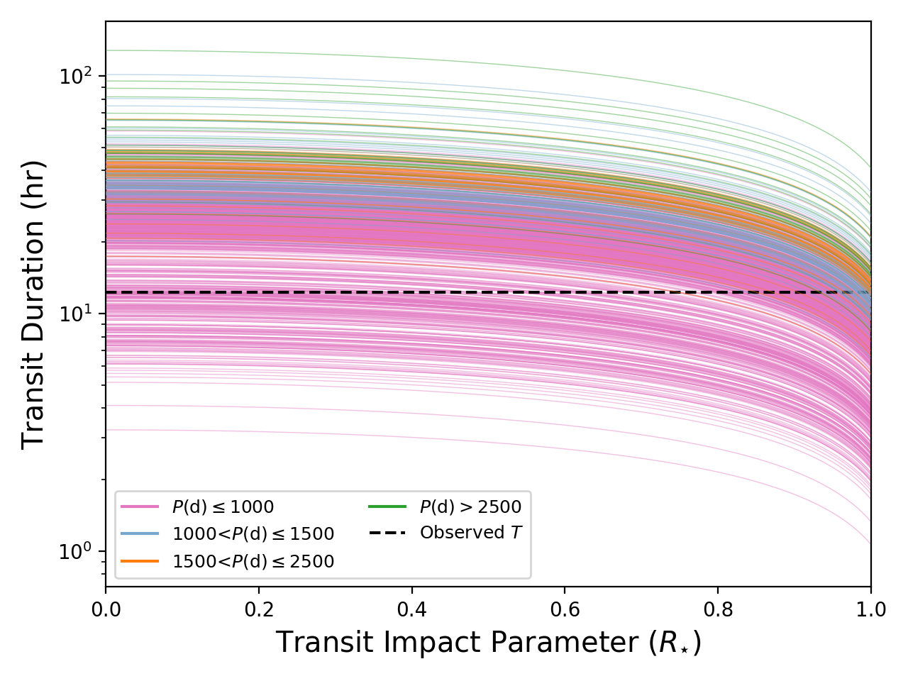
Figure 10: Transit duration ($T$) as a function of impact parameter for the solutions to the potential planetary RV signal that are consistent with the Kepler occultation. The duration of the occultation observed by Kepler (Figure 2) is indicated. We find that 1 $R_{\rm Jup}$ objects that have solutions with $P>1500$ days are incapable of producing the observed occultation regardless of the impact parameter.

5.1.1 Visualizing the RV Time Series

The RV time series of the potential giant planet or brown dwarf companion can also be modeled using the posterior PDFs. We randomly draw 1000 samples from the posterior PDFs of all solutions and calculate their RV time series (Figure 11, top panel). For each draw, the median value of the $\dot{\gamma}$ posterior is used to remove the long-term RV trend from the model time series. The median and 68% confidence region for $\dot{\gamma}$ is $-7.05^{+0.06}_{-0.07}$ m s^-1 day^-1. The same procedure is also applied to the Keck-HIRES data. We use the lower limit of the orbital period (687 days; see Figure 9) to distinguish between long-period solutions that are consistent with the Kepler occultation and short-period solutions that are not.

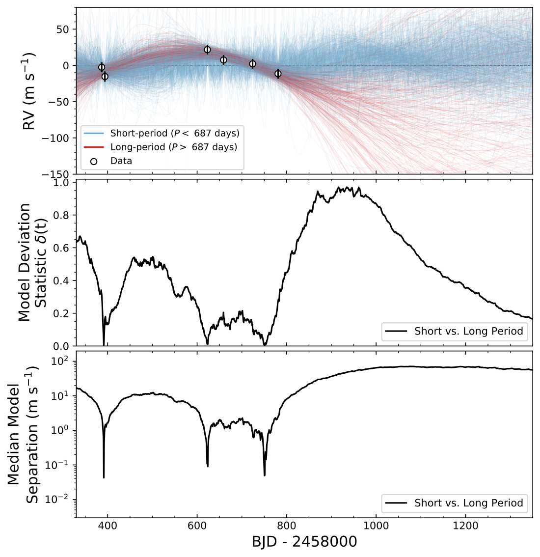
Figure 11: Top: model RV time series of the potential planetary RV signal based on 1000 random draws from the posterior PDFs of all solutions. The Keck-HIRES data are shown as open circles. Middle: the model deviation statistic time series comparing the long-period solutions (red) that are consistent with the Kepler occultation and short-period solutions (blue) that are not. The most useful time to make an observation that distinguishes between groups of solutions was before BJD = 2459000. Bottom: the absolute RV separation between the median time series of each group of solutions.

To aid in predicting future observations that distinguish between groups of solutions, we define a time-dependent model deviation statistic $\delta$

$$\delta(t)=\frac{|M_{\rm short}(t)-M_{\rm long}(t)|}{\sqrt{\sigma_{\rm short}(t)^{2}+\sigma_{\rm long}(t)^{2}}}$$ (8)

where $M_{\rm short}$ and $M_{\rm long}$ are the median RV time series models of the short- and long-period groups of solutions, respectively, $\sigma_{\rm short}$ and $\sigma_{\rm long}$ are the standard deviation time series of the RV models within the short- and long-period groups of solutions, and $t$ is time. This statistic is the difference between two models weighted by the combined spread within each of those models. It is effectively a S/N ratio for the deviation between models. Values of $\delta(t)$ greater than unity highlight strategic times to obtain observations that distinguish between groups of solutions.

As shown in Figure 11, $\delta\approx 1$ between BJD = 2458900 and BJD = 2459000. After this brief period, which has already passed, the short- and long-period model groups mix such that $\delta$ remains below unity for the near-term future. In general, this means that a single observation will likely not distinguish between model groups or, by extension, constrain the nature of the companion that caused the Kepler occultation. The bottom panel of Figure 11 displays the absolute velocity separation between the median time series of the short- and long-period model groups. This suggests that the level of precision yielded by the matched-template technique is sufficient for future observations of this target.

5.2 The Long-term RV Trend

We now investigate the long-term RV trend (Figure 8, top panel) with another rejection sampling analysis. Here, we do not include a parameter for first-order acceleration. Instead, the data are treated as if they cover only a fraction of the phase of a longer signal. We effectively mask the potential planetary signal by increasing the error bars of the Keck-HIRES data by a factor of four. This increase makes the new median error (of $\sim$27 m s^-1) consistent with the peak of the potentially planetary semiamplitude posterior PDF (Figure 9). If we do not increase the data error, the rejection sampling cannot robustly sample the posterior PDFs of the model parameters merely because the model likelihood for all samples is low.

For this rejection sampling analysis, the lower bound on the orbital period prior is set to the observational baseline ($P_{\rm min}=394$ days) since the data clearly do not span a full orbit. The choice of an upper bound for this prior is less straightforward. The high degree of linearity of the precise Keck-HIRES RVs is consistent with a broad range of long periods. However, we can constrain the RV variation of KIC 5951458 with its RV measurements from the Gaia mission (Gaia Collaboration et al., 2018; Katz et al., 2019). Between 2014 July 25 (BJD = 2456863.5) and 2016 May 23 (BJD = 2457531.5), Gaia acquired 11 absolute RV measurements of KIC 5951458. These individual measurements are yet unpublished, but the Gaia Data Release 2 included their median value ($-23.0\pm 1.3$ km s^-1) and the corresponding epoch (2015.5 or BJD = 2457204.5). This Gaia RV can be compared to the telluric-calibrated, absolute RVs produced from the HIRES spectra by the methodology of Chubak et al. (2012), which we list in Table 4. Using standard stars, Soubiran et al. (2018) found excellent agreement between the Gaia RVs and the catalog of Chubak et al. (2012), quantified by a dispersion of only 0.072 km s^-1, which is much lower than the error on the Gaia RV measurement of KIC 5951458. In Figure 12, we show the Gaia RV and the Keck-HIRES telluric RVs of KIC 5951458. It is clear that the linear trend of the Keck-HIRES data must turn over in order for these data to be consistent with the measurement from Gaia. This suggests that we can derive an upper limit on the orbital period of the companion causing the long-term trend.

Figure 12: Absolute, telluric-calibrated RVs from Keck-HIRES (black points) and median RV measurement spanning BJD = 2456863.5–2457531.5 from Gaia (red point). The Gaia measurement shows that the linear trend of the Keck-HIRES data must turn over, thereby setting an upper limit on the orbital period of the companion causing the trend ($P_{\rm max}\approx 13,000$ days). The gray lines are 500 time series created by randomly drawing solutions from a rejection sampling analysis of these RVs.

To derive an upper limit on the orbital period of the companion causing the long-term trend, we conduct a simple rejection sampling analysis on the joint Keck-Gaia RV data set using The Joker. We bound the orbital period prior at 394 days and 1$\,\times\,10^{6}$ days and sample the posterior $2^{21}$ times. From the resulting posterior PDF for orbital period, we calculate the 99.7th percentile to be $\sim$13,000 days. We treat this value as the maximum orbital period of the companion causing the long-term trend.

With the orbital period prior bounded at $P_{\rm min}=394$ days and $P_{\rm max}=13,000$ days, we proceed with the rejection sampling analysis on just the precise Keck-HIRES RVs calculated using the matched-template analysis. We use The Joker to sample the prior PDFs $2^{21}$ times. Of these, 39,666 samples of the posterior PDFs survive.

The marginal posterior PDFs for $P$ and $K$ from all solutions are shown in Figure 13. The PDFs for $K$ and $P$ are smooth, although the latter truncates at 13,000 days owing to the prior. The shortest-period solutions are on the order of 420 days. We also derive and display the posterior PDFs from all solutions for orbital semi-major axis ($a$) and the companion minimum mass ($M\sin{i}$). In doing so, we solve for $M\sin{i}$ numerically and do not assume that the companion mass is negligible compared to the host mass. The $M\sin{i}$ posterior PDF truncates at high values as a result of the minimum possible values of $K$ set by the span of the RV data.

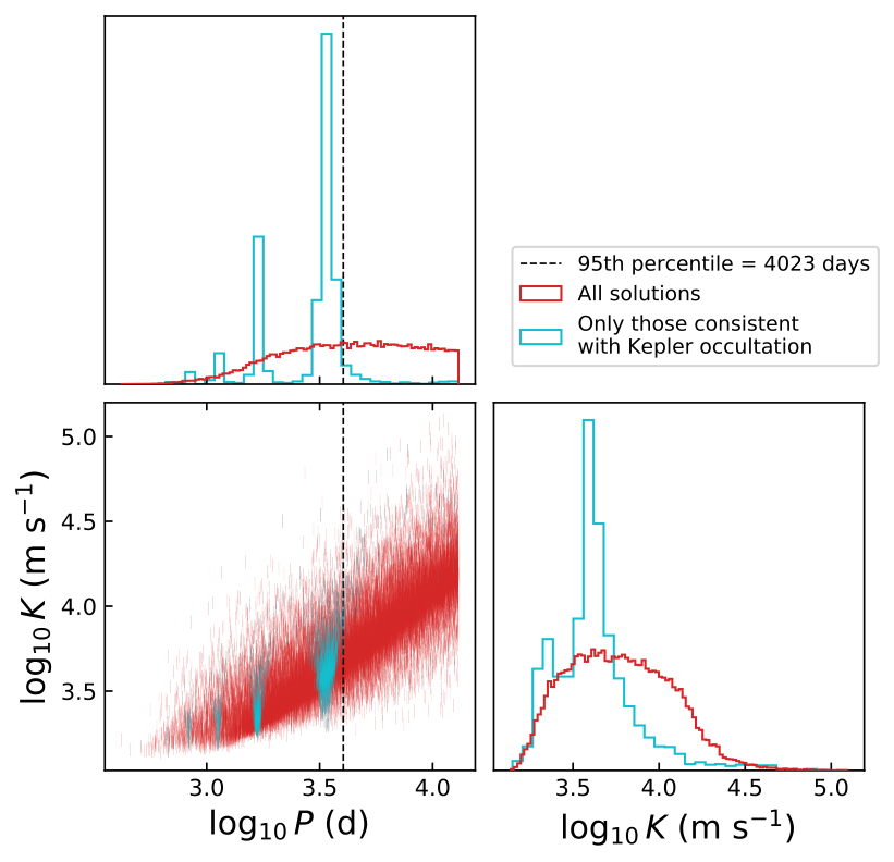
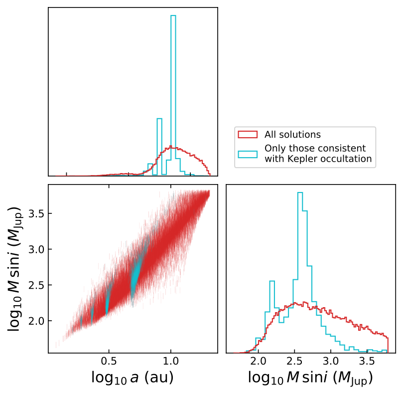
Figure 13: Left panels: marginal posterior PDFs for orbital period ($P$) and RV semiamplitude ($K$) from the rejection sampling of the long-term RV trend. The dashed line shows the 95th percentile in orbital period for solutions that are consistent with the Kepler occultation (cyan). Right panels: marginal posterior PDFs for the derived parameters companion minimum mass ($M\sin{i}$) and orbital semi-major axis ($a$). Both groups of panels show the posteriors from all solutions (red), as well as the subset consistent with the Kepler occultation (cyan). For the latter, 95% of solutions have $M\sin{i}=95-1659\;M_{\rm Jup}$ and $P<4023$ days, suggesting that the companion would likely be a star.

As in Section 5.1, it is informative to identify the subset of the posterior PDF that is consistent with the occultation observed by Kepler. We again compare each solution’s inferior conjunction time with the time of the Kepler occultation as described in Section 5.1. We present the posterior PDFs from only those solutions that are consistent with the Kepler occultation in Figure 13. The histograms in this figure have each been normalized such that they integrate to unity. This posterior PDF for $P$ is multimodal, with distinct peaks at $\sim 1700$ and $\sim 3400$-days. The 95th percentile in orbital period for solutions that are consistent with the Kepler occultation is 4023 days. The posterior PDF for $M\sin{i}$ is broad and also multimodal with peaks at $\sim 155$ and $\sim 400$ $M_{\rm Jup}$. Both of these cases, and the vast majority of all solutions, suggest that the companion causing the long-term trend is stellar in nature.

5.2.1 Visualizing the RV Time Series

We model the RV time series of the stellar companion causing the long-term trend in the RVs. We randomly draw 1000 samples from the posterior PDFs of all the solutions and calculate their RV time series (Figure 14, top panel). We use the upper limit of the orbital period (4023 days; see Figure 13) to distinguish between short-period solutions that are consistent with the Kepler occultation and long-period solutions that are not. From the median RV times series of short- and long-period groups of solutions, we calculate the RV separation and the model deviation statistic $\delta(t)$. As derived in Section 5.1.1, $\delta(t)$ is the time-dependent difference between median models weighted by the uncertainty in that difference. The middle panel of Figure 14 shows a broad peak in $\delta(t)$ near BJD${}_{\rm TDB}=$ 2460000. This peak and subsequent turnover demonstrate how the divergence between the short- and long-period models is eventually overcome by the increasing uncertainty within each group. The bottom panel of Figure 14 shows that the RV separation between the model groups is substantial ($\sim$10 km s^-1) near the peak in $\delta(t)$.

Figure 14: Top: model RV time series of the long-term RV trend for KIC 5951458 based on 1000 random draws from the posterior PDF. The Keck-HIRES data are the open black circles. The short- and long-period solutions are divided at $P=4023$ days, which is the 95th percentile in orbital period for solutions consistent with the Kepler occultation. Middle: the model deviation statistic time series (Section 5.1.1). The broad peak represents a balance between the divergence of short- and long-period models and the increasing uncertainty within each model group. Bottom: The absolute RV separation between median short- and long-period models.

The information displayed in Figure 14 suggests that the optimal time to obtain another RV epoch of KIC 5951458 is near BJD = 24560000 (2023 February). At that time, the short- and long-period model groups will be substantially separated such that a single, high-precision RV measurement could likely distinguish between them and, by extension, constrain the nature of the companion that caused the occultation seen by Kepler.

5.3 Results of the Rejection Sampling Analysis

The rejection sampling analysis of the previous sections is meant to characterize the signals in the sparse set of RV observations and enable an informed interpretation of the single occultation event detected in Quarter 4 of the Kepler primary mission. We find that there are two distinct signals in the RV data. The first signal is a several kilometers-per-second trend from what is likely a stellar companion. The posterior PDF for the minimum mass of this companion is too broad to determine its exact nature, but it is highly unlikely to be planetary. Its orbital period is likely longer than $\sim$1000 days, but not so long that we would expect it to have been detected by the AO imaging (Figure 3). The depth and duration of the occultation event from Kepler are consistent with the properties of this companion, but only if its orbital period is less than $\sim$4023 days or likely either $\sim 1700$ or $\sim$3400 days. If this companion’s orbital period is substantially greater than $\sim$4023 days, then only very fine-tuned combinations of orbital parameters would have allowed it to have passed through inferior conjunction during Quarter 4 of the primary Kepler mission.

Using the RV time series and the model deviation statistic in Figure 14, we predict that just one additional RV epoch acquired in the 2022 or 2023 Kepler observing seasons (surrounding 2460000 BJD) would be particularly helpful in the interpretation of the KIC 5951458 system. At that time, the short-period solutions (which are consistent with the occultation) and the long-period solutions (which are not) will have sufficiently diverged to be able to distinguish between the two. If this RV observation follows the long-period solutions (i.e., the red curves in Figure 14), then the Kepler occultation was likely not caused by the stellar companion. If the RV observation lands in between the two groups or toward the short-period groups, then the stellar companion still may have caused the occultation event. In this case, many additional observations will be necessary to characterize the system.

The second signal in the RV data is that of a potential giant planet or brown dwarf. This signal is seen when the large linear trend is removed (Figure 8, bottom panel). There are several somewhat discrete groups of possible orbital periods for this companion, many of which are shorter than 1000 days. A total of 88% of the solutions qualify this companion as a giant planet with minimum mass in the range of 0.3–13 $M_{\rm Jup}$. Assuming a typical 1 $R_{\rm Jup}$ radius, this planetary or brown dwarf companion is capable of producing the occultation event observed by Kepler. Also, the fact that this companion likely orbits closer to KIC 5951458 than the stellar companion means that it is geometrically more likely to have caused the occultation. However, based on the date of the occultation, its duration, and the nondetection of a second event in the full Kepler data set, the planetary or brown dwarf companion must have an orbital period in the range of $\sim$687–1500 days to have caused the occultation event. This suggests that it would be worthwhile to obtain several RVs to distinguish between various long-period solutions (as described in Section 5.1) and then conduct follow-up photometric monitoring to detect an additional transit.

6 Discussion

We found that the story of KIC 5951458 b—a member of the confirmed exoplanets list—is more complicated than previously thought. Although we cannot uniquely determine the full nature and architecture of the KIC 5951458 system, we know that the current description of KIC 5951458 b as it stands in the list of confirmed exoplanets is incorrect. KIC 5951458 likely hosts a substellar-mass companion with an orbital period less than or around a few thousand days. It could be a giant planet or a brown dwarf, and its radius is unknown because it may not transit its host star.

Despite the uncertainty pertaining to the nature and architecture of the KIC 5951458 system, the scientific potential surrounding the future characterization of this system remains high. Regardless of which object caused the occultation event observed by Kepler, KIC 5951458 appears to be a binary star system where the primary hosts a giant planet or brown dwarf. If we assume the former, this system would join a relatively small group of circumprimary exoplanets, which are useful for probing the extremes of planet formation, as well as for comparison to single-star planetary systems (e.g., Thebault & Haghighipour, 2015, and references therein). Even within the sample of known circumprimary exoplanets, KIC 5951458 b would be quite interesting. To date, only three systems (Kepler-420, (Santerne et al., 2014); Kepler-693, (Masuda, 2017); and HD 42936, (Barnes et al., 2019)) are known to have a circumprimary planet and a secondary star within 10 au.

The KIC 5951458 system becomes even more interesting when we consider which companion caused the Kepler occultation event. If the stellar companion caused the occultation, then KIC 5951458 joins the list of known eclipsing binaries (EBs). Assuming that the binary orbital period is $\sim$3400 days (the highest peak in Figure 13), KIC 5951458 would rank in the 99.9th percentile by period among other EBs (Malkov et al., 2006). According to the Kepler Eclipsing Binary Catalog (e.g., Prša et al., 2011), KIC 5951458 would become the longest-period Kepler EB if its period were 3400 days or even the alias at half of that value. With additional refinement of the binary star ephemeris, future eclipse observations would be particularly useful to characterizing this system.

Alternatively, the scenario in which the giant planet or brown dwarf companion caused the occultation event is perhaps even more tantalizing. To be consistent with the impact parameter measured by Kawahara & Masuda (2019), this object likely has an orbital period between 687 and 1500 days. This alone would make it a remarkable exoplanet or brown dwarf, since the geometric bias of the transit method so severely limits detections to short-period objects. Long-period transiting exoplanets are a valuable pathway toward characterizing the atmospheres, interiors, and formation histories of cooler planets that more resemble the solar system (e.g., Dalba et al., 2015; Dalba & Tamburo, 2019). Conducting future photometric observations to detect additional occultations would be useful for measuring the bulk density of KIC 5951458 b, be it a planet or brown dwarf, and for drawing further conclusions on its formation and evolution.

Finally, the evolving nature of the narrative describing the KIC 5951458 system is one that will become more common due to the ongoing transit hunting efforts of TESS (Ricker et al., 2015). TESS is predicted to discover on the order of 1000 single-transit events in its primary mission alone (Villanueva et al., 2019; Dalba et al., 2020; Eisner et al., 2020; Gill et al., 2020). The need to conduct imaging, photometric, and spectroscopic follow-up for many of these discoveries will place an immense burden on the pool of observational resources available to the exoplanet community.

In this work, we have utilized archival data and collected only a small amount (i.e., six RV epochs) of new follow-up data of KIC 5951458. We then conducted an exploratory study of the degeneracies between interpretations of the system’s nature and architecture. This has led to predictions for future observations of this system. An alternate approach would have been to acquire as many RV observations as possible over a full orbit. This approach is commonly applied in exoplanet characterization endeavors, although most transiting exoplanets followed up with RVs have much shorter orbital periods than the companions orbiting KIC 5951458. Moving forward, we argue that the conservative approach—whereby degeneracies in the interpretation of the system are identified and the timing of efficient follow-up opportunities is determined—will become increasingly valuable for the characterization of single-transit planet candidates. The deluge of TESS short-period planet discoveries places a strain on existing RV facilities. Attempts to observe single-transit planet candidates—one of the only avenues to long-period exoplanets suitable for detailed characterization—must find a way to complement efforts to observe shorter-period planets. Our conservative approach is one option, and we have demonstrated its usefulness for the KIC 5951458 system in this work.

7 Summary

We described two novel techniques surrounding the analysis of precise RVs of a supposed exoplanet hosting system KIC 5951458. The first technique pertains to the extraction of the RVs of KIC 5951458, a 13th-magnitude F5 star previously observed by the primary Kepler mission. To extract precise RVs for this star, we developed a novel matched-template technique that leverages the collection of several hundred high-S/N iodine-free spectra acquired with Keck-HIRES (Section 4). This technique matches a new target star to a current member of the template library and uses its preexisting template to extract precise RVs. Using this method, we were able to forgo the collection of a new iodine-free template spectrum for KIC 5951458, which would have required an expensive investment of time. We found that the RV uncertainty incurred by the matched-template technique (in addition to internal RV errors) is 4–8 m s^-1 for most stars that would be subject to precise RV observations (Figure 6). In Section 4.1, we provide a procedure for determining the suitable error to add to the internal RVs for different types of stars. In general, the matched-template technique will produce RVs that are precise and accurate enough to investigate giant planet signals and to aid in the planning of additional observations.

The second novel technique described in this work surrounds the analysis of a single-transit exoplanet candidate through the synthesis of sparse collections of imaging, photometric, and spectroscopic data. KIC 5951458 was previously thought to host a long-period transiting exoplanet based on a single occultation event detected in Quarter 4 of the Kepler primary mission (Wang et al., 2015; Kawahara & Masuda, 2019). We used the rejection sampling tool The Joker (Price-Whelan et al., 2017) to model the RV observations of KIC 5951458 and explore the possible explanations for the nature of the system. We found that the published parameters for the confirmed planet KIC 5951458 b are incorrect and that the KIC 5951458 system is substantially more complicated than originally thought.

The RVs of KIC 5951458 show a large trend that is indicative of a stellar companion with an orbital period longer than a few thousand days. In addition to the RV trend, there also exists a signal likely caused by a giant planet or brown dwarf companion with mass in the range of 0.6–82 $M_{\rm Jup}$ and orbital period less than a few thousand days. Based on these findings, we cannot clearly identify which companion to KIC 5951458 caused the occultation event detected by Kepler. If the occultation was caused by the giant planet or brown dwarf, then we can further constrain its orbital period to be between $\sim$687 and $\sim$1500 days. Alternatively, if the stellar companion caused the occultation, we can further constrain its orbital period to be less than 4023 days, and likely either $1700$ or $3400$ days.

We offer predictions to be tested by future observations that can distinguish between possible scenarios for the architecture of the KIC 5951458 system. Regardless of which scenario is correct, we explain why KIC 5951458 is a rare and unlikely system worthy of follow-up characterization. Lastly, we argue that investigations conducted after only a small amount of follow-up data have been collected will be critical to maximizing the science return from single-transit objects detected by Kepler and TESS.

References

- Bailer-Jones et al. (2018) Bailer-Jones, C. A. L., Rybizki, J., Fouesneau, M., Mantelet, G., & Andrae, R. 2018, AJ, 156, 58, doi: 10.3847/1538-3881/aacb21
- Barclay et al. (2013) Barclay, T., Burke, C. J., Howell, S. B., et al. 2013, ApJ, 768, 101, doi: 10.1088/0004-637X/768/2/101
- Barnes et al. (2019) Barnes, J. R., Haswell, C. A., Staab, D., et al. 2019, Nature Astronomy, 505, doi: 10.1038/s41550-019-0972-z
- Borucki et al. (2010) Borucki, W. J., Koch, D., Basri, G., et al. 2010, Science, 327, 977, doi: 10.1126/science.1185402
- Chubak et al. (2012) Chubak, C., Marcy, G., Fischer, D. A., et al. 2012, arXiv e-prints, arXiv:1207.6212. https://arxiv.org/abs/1207.6212
- Coelho et al. (2005) Coelho, P., Barbuy, B., Meléndez, J., Schiavon, R. P., & Castilho, B. V. 2005, A&A, 443, 735, doi: 10.1051/0004-6361:20053511
- Crossfield et al. (2016) Crossfield, I. J. M., Ciardi, D. R., Petigura, E. A., et al. 2016, ApJS, 226, 7, doi: 10.3847/0067-0049/226/1/7
- Cui et al. (2012) Cui, X.-Q., Zhao, Y.-H., Chu, Y.-Q., et al. 2012, Research in Astronomy and Astrophysics, 12, 1197, doi: 10.1088/1674-4527/12/9/003
- Dalba et al. (2017) Dalba, P. A., Muirhead, P. S., Croll, B., & Kempton, E. M.-R. 2017, AJ, 153, 59, doi: 10.1088/1361-6528/aa5278
- Dalba et al. (2015) Dalba, P. A., Muirhead, P. S., Fortney, J. J., et al. 2015, ApJ, 814, 154, doi: 10.1088/0004-637X/814/2/154
- Dalba & Tamburo (2019) Dalba, P. A., & Tamburo, P. 2019, ApJ, 873, L17, doi: 10.3847/2041-8213/ab0bb4
- Dalba et al. (2020) Dalba, P. A., Gupta, A. F., Rodriguez, J. E., et al. 2020, arXiv e-prints, arXiv:2003.10451. https://arxiv.org/abs/2003.10451
- Eisner et al. (2020) Eisner, N. L., Barragán, O., Aigrain, S., et al. 2020, MNRAS, doi: 10.1093/mnras/staa138
- Fulton et al. (2015) Fulton, B. J., Collins, K. A., Gaudi, B. S., et al. 2015, ApJ, 810, 30, doi: 10.1088/0004-637X/810/1/30
- Gaia Collaboration et al. (2018) Gaia Collaboration, Brown, A. G. A., Vallenari, A., et al. 2018, A&A, 616, A1, doi: 10.1051/0004-6361/201833051
- Gill et al. (2020) Gill, S., Wheatley, P. J., Cooke, B. F., et al. 2020, arXiv e-prints, arXiv:2005.00006. https://arxiv.org/abs/2005.00006
- Howard & Fulton (2016) Howard, A. W., & Fulton, B. J. 2016, PASP, 128, 114401, doi: 10.1088/1538-3873/128/969/114401
- Howard et al. (2010) Howard, A. W., Johnson, J. A., Marcy, G. W., et al. 2010, ApJ, 721, 1467, doi: 10.1088/0004-637X/721/2/1467
- Howell et al. (2014) Howell, S. B., Sobeck, C., Haas, M., et al. 2014, PASP, 126, 398, doi: 10.1086/676406
- Isaacson & Fischer (2010) Isaacson, H., & Fischer, D. 2010, ApJ, 725, 875, doi: 10.1088/0004-637X/725/1/875
- Katz et al. (2019) Katz, D., Sartoretti, P., Cropper, M., et al. 2019, A&A, 622, A205, doi: 10.1051/0004-6361/201833273
- Kawahara & Masuda (2019) Kawahara, H., & Masuda, K. 2019, AJ, 157, 218, doi: 10.3847/1538-3881/ab18ab
- Kipping (2013) Kipping, D. M. 2013, MNRAS, 434, L51, doi: 10.1093/mnrasl/slt075
- Latham et al. (2002) Latham, D. W., Stefanik, R. P., Torres, G., et al. 2002, AJ, 124, 1144, doi: 10.1086/341384
- Lightkurve Collaboration et al. (2018) Lightkurve Collaboration, Cardoso, J. V. d. M., Hedges, C., et al. 2018, Lightkurve: Kepler and TESS time series analysis in Python, Astrophysics Source Code Library. http://ascl.net/1812.013
- Luo et al. (2015) Luo, A. L., Zhao, Y.-H., Zhao, G., et al. 2015, Research in Astronomy and Astrophysics, 15, 1095, doi: 10.1088/1674-4527/15/8/002
- Malkov et al. (2006) Malkov, O. Y., Oblak, E., Snegireva, E. A., & Torra, J. 2006, A&A, 446, 785, doi: 10.1051/0004-6361:20053137
- Marcy & Butler (1992) Marcy, G. W., & Butler, R. P. 1992, PASP, 104, 270, doi: 10.1086/132989
- Masuda (2017) Masuda, K. 2017, AJ, 154, 64, doi: 10.3847/1538-3881/aa7aeb
- Morton et al. (2016) Morton, T. D., Bryson, S. T., Coughlin, J. L., et al. 2016, ApJ, 822, 86, doi: 10.3847/0004-637X/822/2/86
- Murray & Dermott (1999) Murray, C. D., & Dermott, S. F. 1999, Solar system dynamics (Cambridge University Press: Cambridge)
- Nidever et al. (2002) Nidever, D. L., Marcy, G. W., Butler, R. P., Fischer, D. A., & Vogt, S. S. 2002, ApJS, 141, 503, doi: 10.1086/340570
- Petigura (2015) Petigura, E. A. 2015, PhD thesis, University of California, Berkeley
- Petigura et al. (2017) Petigura, E. A., Howard, A. W., Marcy, G. W., et al. 2017, AJ, 154, 107, doi: 10.3847/1538-3881/aa80de
- Price-Whelan et al. (2017) Price-Whelan, A. M., Hogg, D. W., Foreman-Mackey, D., & Rix, H.-W. 2017, ApJ, 837, 20, doi: 10.3847/1538-4357/aa5e50
- Prša et al. (2011) Prša, A., Batalha, N., Slawson, R. W., et al. 2011, AJ, 141, 83, doi: 10.1088/0004-6256/141/3/83
- Ricker et al. (2015) Ricker, G. R., Winn, J. N., Vanderspek, R., et al. 2015, JATIS, 1, 014003, doi: 10.1117/1.JATIS.1.1.014003
- Santerne et al. (2014) Santerne, A., Hébrard, G., Deleuil, M., et al. 2014, A&A, 571, A37, doi: 10.1051/0004-6361/201424158
- Savitzky & Golay (1964) Savitzky, A., & Golay, M. J. E. 1964, Analytical Chemistry, 36, 1627
- Soubiran et al. (2018) Soubiran, C., Jasniewicz, G., Chemin, L., et al. 2018, A&A, 616, A7, doi: 10.1051/0004-6361/201832795
- Thebault & Haghighipour (2015) Thebault, P., & Haghighipour, N. 2015, Planet Formation in Binaries (Springer, Berlin, Heidelberg), 309–340, doi: 10.1007/978-3-662-45052-9_13
- Thompson et al. (2018) Thompson, S. E., Coughlin, J. L., Hoffman, K., et al. 2018, ApJS, 235, 38, doi: 10.3847/1538-4365/aab4f9
- Twicken et al. (2016) Twicken, J. D., Jenkins, J. M., Seader, S. E., et al. 2016, AJ, 152, 158, doi: 10.3847/0004-6256/152/6/158
- Villanueva et al. (2019) Villanueva, Steven, J., Dragomir, D., & Gaudi, B. S. 2019, AJ, 157, 84, doi: 10.3847/1538-3881/aaf85e
- Vogt et al. (1994) Vogt, S. S., Allen, S. L., Bigelow, B. C., et al. 1994, in Proc. SPIE, Vol. 2198, Instrumentation in Astronomy VIII, ed. D. L. Crawford & E. R. Craine, 362, doi: 10.1117/12.176725
- Wang et al. (2015) Wang, J., Fischer, D. A., Barclay, T., et al. 2015, ApJ, 815, 127, doi: 10.1088/0004-637X/815/2/127
- Winn (2010) Winn, J. N. 2010, in Exoplanets, ed. S. Seager (Tucson: Univ. of Arizona Press), 55–77
- Wizinowich et al. (2000) Wizinowich, P., Acton, D. S., Shelton, C., et al. 2000, PASP, 112, 315, doi: 10.1086/316543
- Wright et al. (2004) Wright, J. T., Marcy, G. W., Butler, R. P., & Vogt, S. S. 2004, ApJS, 152, 261, doi: 10.1086/386283
- Yee et al. (2017) Yee, S. W., Petigura, E. A., & von Braun, K. 2017, ApJ, 836, 77, doi: 10.3847/1538-4357/836/1/77