Exact Solutions of the Time Derivative Fokker-Planck Equation: A Novel Approach

Abstract: In the present article, an approach to find the exact solution of the fractional Fokker-Planck equation is presented. It is based on transforming it to a system of first-order partial differential equation via Hopf transformation, together with implementing the extended unified method. On the other hand, reduction of the fractional derivatives to non autonomous ordinary derivative. Thus the fractional Fokker-Planck equation is reduced to non autonomous classical ones. Some explicit solutions of the classical, fractional time derivative Fokker-Planck equation, are obtained . It is shown that the solution of the Fokker-Planck equation is bi-Gaussian’s. It is found that high friction coefficient plays a significant role in lowering the standard deviation. Further, it is found the fractionality has stronger effect than fractality. It is worthy to mention that the mixture of Gaussian’s is a powerful tool in machine learning. Further, when varying the order of the fractional time derivatives, results to slight effects in the probability distribution function. Also, it is shown that the mean and mean square of the velocity vary slowly.

Keywords: Reduction of fractional derivatives; Non autonomous Fokker-Planck equation; Exact solutions; Extended unified method; Mixed-Gaussian’s

1 Introduction

The Fokker-Planck equation (FPE) deals with fluctuations of systems which stem from disturbances, each of which changes the variables of the system in an unpredictable way. When macroscopic particles are immersed in fluid, they are pulled by the fluid and the position of particles is an unpredictable. So that they fluctuate about an expected position with a certain probability to find the particle in a given region. The probability density function can be determined via the FPE.This equation is used in many different fields in natural science, in solid-state physics, quantum optics, chemical physics, and mathematical biology. Anomalous diffusion is an eminent behavior and characterizes the transport processes of problem in several models [1–4].The features of diffusion can be classified to sub- and super- diffusion. They may be measured by evaluating the variance, relevant to the displacement of particles in the medium, which behaves as $x^{\beta}$where $x$ is the space variable. When $0<\beta<1$, this stands to sub-advection (or in transition state) and when $1<\beta<2$, this case is sub-diffusion (or the transition from advection to diffusion). While in the case when $2<\beta<3$ describes super-diffusion (or the transition from diffusion to dispersion). The first case assigns to spatially disordered or fractal media and also in fractional Brownian motion and random processes [5,  6]. To this end the fractal and fractional time-space derivatives, of orders $\alpha,\,\,0<\alpha<1$ and $\beta,\>1<\beta<2,$ respectively, do emerge in the formulation of diffusion equations relevant to the study of the transport process. By using the time time fractional derivative, the effects of time distributed delay in the transport process are then taken into consideration. While fractal derivative reflect instantaneous frangibility effect.

Fractional derivatives which was proposed in the literature assume numerous definitions; Caputo, Caputo-Fabrizio [7,  8], and a very recently Atangana-Baleneau derivatives [9] and slso Riemann-Liouville, Riesz (see [21]), In the last three, only the kernel of the integral is different depending to when it is singular or not. Analytical investigation of the fractional KPE equation that describes anomalous diffusion of energetic particles [10] are accomplished. An approach was proposed in [11–13] to solve analytically the fractional force-less 1-D FPE. The Klein–Kramers equation (KKE) [14,15] that describes the transport of energetic particles in turbulent magnetic fields are often reduced to the force-less homogeneous one-dimensional FPE.

The KKE [33,  34], which depicts the the Brownian motion of particles in the presence of an outer force $F(z)$ is

$$\frac{\partial}{\partial t}W(t,z,v)=(-v\frac{\partial}{\partial z}+\frac{\partial}{\partial v}(\eta v-\frac{F(z)}{m})+B\frac{\partial^{2}}{\partial v^{2}})W(t,z,v),$$ (1)

where $W(t,z,v)$ is the probability density function of particles, $B=\frac{\eta K_{B}T}{m}$,   $K_{B}$ is the Boltzmann constant, $T$ is the absolute temperature and $m$ is the mass of a diffusing particle, $v$ its velocity, $\eta$ denotes the friction coefficient, $F(z)$ is an external force field.

To depict the distribution in the velocity space, we evaluate the mean and mean square of the particle position in the absence of the external force. In this case, (1) reduces to the FPE that inspect the diffusion of a test particle in the phase space,

$$\frac{\partial}{\partial t}f(t,v)=\eta\frac{\partial}{\partial v}(f(t,v)v)+B\frac{\partial^{2}}{\partial v^{2}}f(t,v),$$ (2)

$f(t,v)=\int_{-\infty}^{\infty}W(t,z,v)dz$ designates the distribution function.

Here, we consider the fractional time KPE of (2) that generalizes the energetic particles transport equations, that is by replacing the ordinary derivatives using the Caputo and Caputo-Fabrizio fractional time derivatives [7,8] to create a prediction of the evolution of the particle distribution function in phase space. We mention that the results obtained incorporate the effects of the distributed time delay.

2 Fractional Derivative

The Caputo fractional derivative (CFD) is defined as follows [21]:

$${}_{0}^{C}D^{\alpha}_{t}f(t)=\frac{1}{\Gamma(m-\alpha)}\int_{0}^{t}(t-t_{1})^{-\alpha+(m-1)}f^{(m)}(t_{1})dt_{1},\>m-1<\alpha<m,\ \ \ t>0,$$ (3)

provided that $f$ is Hoder continuous , $f\epsilon H^{m,\alpha-(m-1)}(\mathbb{R}^{+})$ and the integral exists.

The Caputo-Fabrizio fractional derivative (CFFD) is defined as follows [7]:

$${}_{0}^{CF}D^{\alpha}_{t}f(t)=\frac{2\alpha}{(1-\alpha)(2-\alpha)}\int_{0}^{t}e^{-\frac{\alpha}{1-\alpha}(t-t_{1})}f^{\prime}(t_{1})dt_{1},\ \ 0<\alpha<1,\ \ \ t>0,$$ (4)

provided that $f\epsilon H^{1,\alpha}(\mathbb{R}^{+})$.

The Atangana-Baleanu fractional derivative (ABFD), in the Caputo sense, is defined as follows [9,20]:

$${}_{0}^{AB}D^{\alpha}_{t}f(t)=\frac{B(\alpha)}{1-\alpha}\int_{0}^{t}E_{\alpha}(-\frac{\alpha}{1-\alpha}(t-t_{1})^{\alpha})f^{\prime}(t_{1})dt_{1},\ \ \ 0<\alpha<1,\ \ \ t>0,$$ (5)

where $B(\alpha)>0$ is a normalization function satisfying $B(0)=B(1)=1$ and $E_{\alpha}(t)$ is the Mittag–Leffler function and $f\epsilon H^{1,\alpha}(\mathbb{R}^{+})$. It is worth noticing that this function is not invariant under the CFD. The function which is invariant is $e_{\alpha}(t)$ [26] where

$$E_{\alpha}(t)=\sum_{n=0}^{\infty}\frac{t^{n}}{\Gamma(\alpha n+1)},\ \ \ e_{\alpha}(t):=e_{\alpha,1}(t)=\sum_{n=0}^{\infty}\frac{t^{\alpha n}}{\Gamma(\alpha n+1)},$$ (6)

and the last fractional exponential function generalizes to

$$e_{\alpha,\beta}(\lambda,t)=\sum_{n=0}^{\infty}\frac{\lambda^{n}t^{\alpha n}}{\Gamma(\alpha n+\beta)}.$$ (7)

Here, we propose a new fractional derivative called Gawad’s fractional derivative (GFD) which is defined as follows:

$${}_{0}^{G}D^{\beta}_{t}f(t)=\frac{2\lambda^{\frac{1}{\beta}}}{\lambda+2}\int_{0}^{t}e^{-\lambda(t-t_{1})^{\beta}}f^{\prime}(t_{1})dt_{1},\ \ \beta>0,\ \ \ t>0,$$ (8)

provided that $f\epsilon H^{1,\beta}(\mathbb{R}^{+})$. We mention that the CFFD is a particular case from (8), when $\beta=1$and $\lambda=\frac{\alpha}{1-\alpha}$. The kernel in the fraction derivative (8) is of interest) in the theory of distributions. As when $0<\beta\leq 1$, the fractional exponential distribution is $f(t)=\lambda^{1/\beta}e^{-\lambda t^{\beta}}$generalizes the classical exponential distribution and when $1<\beta\leq 2$, the fractional Gaussian distribution is $f(t)=\frac{\lambda^{1/\beta}}{\sqrt{\pi}}e^{-\lambda t^{\beta}}.$ This later distribution may be considered as transition between the exponential and the Gaussian’s.

2.1 Reduction of the Fractional Derivatives

Here, we shall reduce the fractional derivatives to non autonomous ordinary derivatives, that is with time dependent coefficients [ 22-24].

We consider (3) when $0<\alpha<1,$ is given as follows:

$${}_{0}^{C}D^{\alpha}_{t_{1}}f(t_{1})=\frac{1}{\Gamma(1-\alpha)}\int_{0}^{t_{1}}(t_{1}-t_{2})^{-\alpha}f^{\prime}(t_{2})dt_{2}.$$ (9)

Theorem 2.1.

We assume that the integrand in (9 ) is uniformly integrable on $[0,T_{0}],$ then the CFD is reduced to

$${}_{0}^{C}D^{\alpha}_{t}f(t)=\frac{1}{\Gamma(2-\alpha)}(T_{0}-t)^{1-\alpha}f^{\prime}(t),\ \ \ 0\leq t\leq T_{0}.$$ (10)

$Proof$ In (9), when operating by the integral, over $t_{1}$ on $[0,t]$, it holds that

$$\int_{0}^{t}{{}_{0}^{C}D^{\alpha}_{t_{1}}f(t_{1})}\,dt_{1}=\int_{0}^{t}\Bigg{(}\frac{1}{\Gamma(1-\alpha)}\int_{0}^{t_{1}}(t_{1}-t_{2})^{-\alpha}f^{\prime}(t_{2})dt_{2}\Bigg{)}dt_{1}.\ \$$ (11)

By using the assumption, we permute the inner with the outer integral in the RHS of (11), and have

$$\frac{1}{\Gamma(1-\alpha)}\int_{0}^{t}\Bigg{(}\int_{t_{2}}^{t}(t_{1}-t_{2})^{-\alpha}dt_{1}\Bigg{)}f^{\prime}(t_{2})dt_{2},$$

or

$$\int_{0}^{t}{{}_{0}^{C}D^{\alpha}_{t_{1}}}f(t_{1})dt_{1}=\frac{1}{\Gamma(1-\alpha)}\int_{0}^{t}\frac{(t-t_{2})^{1-\alpha}}{1-\alpha}f^{\prime}(t_{2})\,dt_{2}.$$ (12)

From (12), it holds that

$${}_{0}^{C}D^{\alpha}_{t}f(t)=\frac{1}{\Gamma(2-\alpha)}(T_{0}-t)^{1-\alpha}f^{\prime}(t),\ \ \ 0\leq t\leq T_{0}.$$ (13)

Which is identically (9).$\square$

By using the transformation $f(t):=\tilde{f}(\tau),$ (16) can be rewritten:

$${}_{0}^{C}D^{\alpha}_{t}f(t):=\frac{d}{d\tau}\tilde{f}(\tau),\ \ \tau=\frac{\Gamma(2-\alpha)}{\alpha}(T_{0}^{\alpha}-(T_{0}-t)^{\alpha}).$$ (14)

The equations (10) and (14) are among the main results in this work.

By the same way, we find

$$\begin{array}[]{c}{}_{0}^{CF}D^{\alpha}_{t}f(t)=\frac{2}{(2-\alpha)}\Bigg{(}1-e^{-\frac{\alpha}{1-\alpha}(T_{0}-t)}\Bigg{)}f^{\prime}(t):=\frac{d}{d\tau}\tilde{f}(\tau),\\ \tau=\frac{(2-\alpha)(1-\alpha)}{2\alpha}Log\Bigg{(}\frac{e^{\frac{\alpha}{1-\alpha}(T_{0}-t)}-1}{e^{\frac{\alpha}{1-\alpha}T_{0}}-1}\Bigg{)},\ \ 0\leq t\leq T_{0},\end{array}$$ (15)

$${}_{0}^{AB}D^{\alpha}_{t}f(t)=\frac{B(\alpha)}{(1-\alpha)}(T_{0}-t)e_{\alpha,2}\Bigg{(}-\frac{\alpha}{1-\alpha},(T-t_{1})\Bigg{)}f_{0}^{\prime}(t),$$ (16)

where [25]

$$e_{\alpha,\beta}(\sigma,x)=\sum_{n=0}^{\infty}\frac{\sigma^{n}x^{\alpha n}}{\Gamma(\alpha n+\beta)},$$ (17)

and

$$\begin{array}[]{c}{}_{0}^{G}D^{\beta}_{t}f(t)=\frac{2}{\lambda+2}\gamma(\frac{1}{\beta},\lambda(T_{0}-t)^{\beta})f^{\prime}(t):=\frac{d}{d\tau}\tilde{f}(\tau),\\ \tau=\frac{(\lambda+2)}{2}\int_{0}^{t}\frac{1}{\gamma(\frac{1}{\beta},\lambda(T_{0}-t_{1})^{\beta})}dt_{1},\ \ 0\leq t\leq T_{0},\ \ 0<\beta<1,\end{array}$$ (18)

where $\gamma(m,t)$ is the incomplete lower Gamma function. We mention that

$$\gamma(a,x)+\varGamma(a,x)=\Gamma(a),\ \ \ a>0,\ \ \ x>0,\ \ \ \ \varGamma(a,x)=\int_{x}^{\infty}e^{-y}y^{a-1}dy.$$ (19)

Now, we will prove the following theorem by using (19).

Theorem 2.2.

The GFD satisfies the following:

(i) ${}_{0}^{G}D^{\beta}_{t}(g(t)+f(t))=_{0}^{G}D^{\beta}_{t}g(t)+_{0}^{G}D^{\beta}_{t}f(t)$.

(ii) ${}_{0}^{G}D^{\beta}_{t}(f(t)g(t))=f(t)$${}_{0}^{G}D^{\beta}_{t}g(t)+g(t)_{0}^{G}D^{\beta}_{t}f(t).$

(iii)${}_{0}^{G}D^{\beta}_{t}(\frac{f(t)}{g(t)}))=\frac{g(t)_{0}^{G}D^{\beta}_{t}f(t)-f(t)_{0}^{G}D^{\beta}_{t}g(t)}{g(t)^{2}}$.

Further, by using (19) the function $f(t)$ which is invariant under the GFD and

$${}_{0}^{G}D^{\beta}_{t}e_{\beta,G}(t)=e_{\beta,G}(t),$$

is found directly by:

$$e_{\beta,G}(t)=e^{\frac{(\lambda+2)}{2}\int_{0}^{t}\frac{1}{\gamma(\frac{1}{\beta},\lambda(T_{0}-t_{1})^{\beta})}dt_{1}}.$$ (20)

3 Solutions of the FPE

We present a novel approach to solve of (2) as follows. Here we use the transformations

$$f_{v}(t,v)=F(v,t)\,f(t,v),\ \ \ \ f_{t}(t,v)=G(t,v)\,f(t,v).$$

Thus (2) is rewritten as follows:

$$\begin{array}[]{c}f_{v}(t,v)-F(t,v)\,f(t,v)=0,\ \ \ f_{t}(t,v)-G(t,v)\,f(t,v)=0,\\ G(t,v)-\eta(1+vF(t,v))-B(F_{v}(t,v)+F(t,v)^{2})=0.\end{array}$$ (21)

On the other hand, the unified method is implemented. It asserts that the solutions of partial differential equations (PDEs) can be expressed by a polynomial or a rational forms in an auxiliary functions that satisfy appropriate auxiliary equations. Here, we are concerned with rational forms in the cases of different auxiliary equations. This will be classified in what follows.

3.1 Case of Linear Auxiliary Equations

We write the solutions of (21) in the form.

$$\begin{array}[]{c}f(t,v)=\frac{s_{1}(v)g(t,v)+s_{0}(v)}{a_{1}(v)g(t,v)+a_{0}(v)},\ \ \ F(t,v)=\frac{b_{1}(v)g(t,v)+b_{0}(v)}{s_{1}(v)g(t,v,z)+s_{0}(v)},\\ G(t,v)=\frac{d_{1}(v)g(t,v)+d_{0}(v)}{s_{1}(v)g(t,v)+s_{0}(v)}.\end{array}$$ (22)

We assume that the auxiliary equations are linear,

$$\begin{array}[]{c}g_{t}(t,v)=\mu\,(c_{1}g(t,v)+c_{0}),\ \ \ \ g_{v}(t,v)=h(v)\,(c_{1}g(t,v)+c_{0}).\end{array}$$ (23)

It is worth noticing that in (23), the compatibly equation $g_{tv}(t,v)=g_{vt}(t,v)$ holds.

By inserting (22) and (23) into (21), and by using (24), we get a system of nonlinear algebraic equations in  $a_{i}(v),\ \ b_{i}(v)\ and\ d_{i}(v),$   $i=1,2...\ .$  We found that the calculations are not straight forward due to two facts.
(i)The equations obtained are nonlinear.
(ii) It arises that we can have two equations in the same dependent variable, for example,  $a_{j}(v)$  and  $a_{j}^{\prime}(v),\ \ \ j=0,1,...,$ so, we have to use the compatibly equation, $b_{j}^{\prime}(v)-(b_{j}(v))^{\prime}=0$.

By setting the coefficients of $g(t,v)^{j},\ \ \ j=0,1,...,$ equal to zero, we have the following equations

$$a_{0}^{\prime}(v) =\frac{1}{s_{0}(v)}\Bigg{(}-c_{0}a_{1}(v)h(v)s(v)+a_{0}(v)\Bigg{(}-b_{0}(v)$$

$$+c_{0}h(v)s_{1}(v)+s_{0}^{\prime}(v)\Bigg{)}\Bigg{)},$$

$$s_{1}^{\prime}(v) =b_{1}(v),$$

$$s_{0}^{\prime}(v) =b_{0}(v)+h(v)\Bigg{(}-c_{0}s_{1}(v)+c_{1}s_{0}(v)\Bigg{)},$$ (24)

$$b_{0}^{\prime}(v) =\frac{1}{m\,B}\Bigg{(}b_{0}(v)(-m\,v\,\eta+F_{0}+Bc_{1}mh(v))$$

$$-m\Bigg{(}Bc_{0}b_{1}(v)h(v)-c_{0}(k_{0}v+\mu)s_{1}(v)$$

$$+\Bigg{(}c_{1}k_{0}v+\eta+c_{1}\mu\Bigg{)}s_{0}(v)\Bigg{)}\Bigg{)},$$

$$b_{1}^{\prime}(v) =\frac{1}{m\,B}(b_{1}(v)(-m\,v\,\eta+F_{0})-m\,\eta s_{1}(v)),$$

and

$$\begin{array}[]{c}d_{1}(v)=0,\;d_{0}(v)=\frac{c_{1}\mu}{a_{1}(v)}\Bigg{(}s_{1}(v)-a_{1}(v)s_{0}(v)\Bigg{)},\\ \;a_{1}(v)=c_{1}/c_{0},\ \ \ a_{0}(v)=1.\end{array}$$ (25)

By rewriting the second equation in (24) as   $b_{1}(v)=s_{1}^{\prime}(v),$  the compatibly equation

$$b_{1}^{\prime}(v)-(b_{1}(v))^{\prime}=0,$$

gives rise to

$$m\,\eta s_{1}(v)+mv\eta s_{1}^{\prime}(v)+B\,ms_{1}^{\prime\prime}(v)=0,$$ (26)

where (26) solves to

$$\begin{array}[]{c}s_{1}(v)=A_{2}e^{-\frac{v^{2}\eta}{2\,B}}+A_{1}\sqrt{\frac{\pi\,B}{2\eta}}e^{\frac{v^{2}\eta}{2\,B}-\frac{F_{0}^{2}}{2Bm^{2}\eta}}erfi(\frac{m\,v\,\eta}{\sqrt{2B\eta}m}),\\ erfi(x)=e^{-x^{2}}\int_{0}^{x}e^{y^{2}}dy.\end{array}\;$$ (27)

Thus, we can evaluate $b_{1}(v)=s_{1}^{\prime}(v).$
By the same way, we rewrite the third equation in (24) as

$$b_{0}(v)=-s_{0}^{\prime}(v)+h(v)(-c_{0}s_{1}(v)+c_{1}s_{0}(v)),$$ (28)

we find that the compatibly equation $b_{0}^{\prime}(v)-(b_{0}(v))^{\prime}=0,$ gives rise to:

$$(m\,v\,\eta)h(v)+Bc_{1}mh(v)^{2}+m(+\mu-Bh^{\prime}(v))=0.$$ (29)

The solutions of (29) gives rise to :

$$\begin{array}[]{c}c_{1}=\frac{n\,\eta}{\mu},\ \ \ h(v)=\frac{P_{1}(v)}{Q_{1}},\ \ \ P_{1}(v)=-\sqrt{\frac{2B}{\eta}}\mu B_{0}H_{n-1}\Bigg{(}\frac{v\sqrt{\eta}}{\sqrt{2B}}\Bigg{)}\\ +v\mu_{1}F_{1}\Bigg{(}1-\frac{n}{2},\frac{3}{2},\frac{v^{2}\eta}{2B}\Bigg{)},\\ Q_{1}(v)=BB_{0}H_{n}(\frac{v\sqrt{\eta}}{\sqrt{2B}})+{}_{1}F_{1}\Bigg{(}-\frac{n}{2},\frac{1}{2},\frac{\eta v^{2}}{2B}\Bigg{)},\end{array}$$ (30)

where $H_{n}(v\sqrt{\frac{\eta}{2B}})$ and ${}_{1}F_{1}(-\frac{n}{2},\frac{1}{2},\frac{\eta v^{2}}{2B})$ are the Hermite polynomial and the hyper geometric functions respectively.

Further the solution of the auxiliary equations give rise to

$$g(v,t)=-\frac{c_{0}}{c_{1}}+B_{3}e^{c_{1}\int h(v)dv+\mu t}.$$ (31)

We mention that$\int h(v)dv$ can not be directly evaluated. To this end we assume that (cf. (30))

$$(Q_{1}+s(v))^{\prime}=P_{1},$$ (32)

and the calculations give

$$\begin{array}[]{c}s(v)=\frac{(n\eta+\mu)}{n\eta}(-BB_{0}H_{n}\Bigg{(}\frac{v\sqrt{\eta}}{\sqrt{2B}}\Bigg{)}+B(1-_{P}F_{Q}(\{-\frac{n}{2}\},\{\frac{1}{2}\},\frac{\eta v^{2}}{2B})),\\ \end{array}$$ (33)

where ${}_{P}F_{Q}$ is the generalized hyper geometric function. Finally, we get

$$\int h(v)dv=Log(\mid P_{1}(v)+s(v)\mid).$$ (34)

By substituting for $s_{i}(v),a_{i}(v)$ and by using (24)-(34) in the first equation in (22) we get the required solution.

$$f(t,v)=\frac{P}{Q},$$

$$P=c_{0}\mu\Bigg{(}e^{-\eta\frac{(1+m^{3}v^{2})}{2Bm^{2}}}(2B_{1}e^{\frac{\eta}{2Bm^{2}}})\eta^{3/2}-\sqrt{\frac{2B}{\pi}}\Bigg{(}2A_{1}Bc_{0}e^{\frac{\eta}{2Bm^{2}}}\Bigg{)}\Bigg{)}m-B_{2}\eta)erfi(\frac{m\,v\,\eta}{\sqrt{2B\eta}m}))$$

$$+\eta^{3/2}e^{-\frac{v^{2}\eta}{2B}}(2A_{2}+A_{1}\sqrt{\frac{2B}{\pi\eta}}erfi(\frac{m\,v\,\eta}{\sqrt{2B\eta}m})g(t,v)),$$

$$Q=2\eta^{3/2}(c_{0}\mu+n\eta g(t,v)),$$ (35)

and

$$g(t,v) =-\frac{c_{0}\mu}{n\eta}+A_{0}e^{n\,t\,\eta+Log(K)}$$

$$K =\frac{1}{n\eta}B\Bigg{(}n\,\eta+\mu-B_{0}\mu H_{n}(v\sqrt{\frac{\eta}{2B}})+n\,\eta\,_{1}F_{1}(-(\frac{n}{2}),\frac{1}{2},\frac{\eta v^{2}}{2B})$$

$$-(n\,\eta+\mu)_{P}F_{Q}\Bigg{(}\{-(\frac{n}{2})\},\{\frac{1}{2}\},\frac{\eta v^{2}}{2B}\Bigg{)}\Bigg{)}.$$ (36)

3.2 Case of Quadratic Auxiliary Equations

We assume that the auxiliary equations are quadratic. We write the solution of (21) in the form

$$\begin{array}[]{c}f(t,v)=\frac{s_{1}g(t,v)+s_{0}}{a_{1}(v)g(t,v)+a_{0}(v)},\>F(t,v)=\frac{b_{1}(v)g(t,v)+b_{0}(v)}{s_{1}g(t,v)+s_{0}},\\ G(t,v)=\frac{d_{1}(v)g(t,v)+d_{0}(v)}{s_{1}g(t,v)+s_{0}},\end{array}$$ (37)

together with auxiliary equation

$$g_{t}(t,v)=\mu\,(c_{2}g(t,v)^{2}+c_{1}g(t,v)+c_{0}),\>g_{v}(t,v)=h(v)\,(c_{2}g(t,v)^{2}+c_{1}g(t,v)+c_{0}).$$ (38)

It is worth noticing that in (38), the compatibility equation $g_{tv}(v,t)=g_{vt}(v,t)$ holds.

By inserting (35) into (21) and by using (38), again we find that the calculations are not straight forward due to two facts.

(i) The equations obtained are nonlinear

(ii) It arises that we can have two equations for $a_{j}(v)$  and  $a_{j}^{\prime}(v),\ \ j=0,1,$   so we have to use the compatibly equation, $a_{j}^{\prime}(v)-(a_{j}(v))^{\prime}=0$. By the same way as in subsection 4.1, we have the following equations

$$a_{0}^{\prime}(v) =\frac{1}{s_{0}}\Bigg{(}-ao(v)bo(v)-c_{0}s_{0}a_{1}(v)h(v)+c_{0}s_{1}a_{0}(v)h(v)\Bigg{)},$$

$$a_{1}^{\prime}(v) =\frac{1}{s_{1}}\Bigg{(}-a_{1}(v)b_{1}(v)-c_{2}s_{0}a_{1}(v)h(v)+c_{2}s_{1}a_{0}(v)h(v)\Bigg{)},$$

$$a_{1}(v) =\frac{a_{0}(v)\Bigg{(}(c_{1}^{2}-k_{0}^{2})s_{1}\mu-4c_{2}d_{0}(v)\Bigg{)}}{\Bigg{(}c_{1}^{2}-k_{0}^{2}\Bigg{)}s_{0}\mu},$$

$$d_{1}(v) =-\frac{\Bigg{(}d_{0}(v)\Bigg{(}(c_{1}^{2}-k_{0}^{2})s_{1}\mu-4c_{1}c_{2}s_{0}\mu-4c_{2}d_{0}[v]\Bigg{)}\Bigg{)}}{\Bigg{(}c_{1}^{2}-k_{0}^{2}\Bigg{)}s_{0}\mu},$$

$$b_{1}(v) =\frac{1}{4c_{2}s_{0}}(4c_{2}s_{1}b_{0}(v)-(c_{1}^{2}-k_{0}^{2})s{}_{1}^{2}h(v)$$

$$+4c_{1}c_{2}s_{1}s_{0}h(v)-4c_{2}{}_{2}^{2}so^{2}h(v),$$

$$d_{0}(v) =-\frac{1}{4c_{2}}\Bigg{(}(c_{1}+k_{0})(-c_{1}s_{1}+k_{0}s_{1}+2c_{2}s_{0})\mu\Bigg{)},$$

$$b_{0}^{\prime}(v) =-\frac{1}{4B^{2}c_{2}h(v)^{2}}(B^{2}c_{2}k_{0}^{2}s_{0}h(v)+c2s_{0}(\mu-Bh^{\prime 2}(v)$$

$$+h(v)^{2}\Bigg{(}c_{2}s_{0}(4B\eta-v^{2}\eta^{2}+2Bk_{0}\mu)+B^{2}\Bigg{(}-c_{1}^{2}s_{1}+k_{0}^{2}s_{1}+2c_{1}c_{2}s_{0}\Bigg{)}h^{\prime}(v)\Bigg{)},$$

$$b_{0}(v) =\frac{1}{4Bc_{2}h(v)}\Bigg{(}2c_{2}s_{0}\mu-2c_{2}s_{0}v\eta h(v)+Bc12s_{1}h^{2}(v)-Bk_{0}2s1h^{2}(v)$$

$$-2Bc_{1}c_{2}s_{0}h^{2}(v)-2Bc_{2}s_{0}h^{\prime}(v)\Bigg{)},\ \ \ c_{0}=\frac{c_{1}^{2}-k_{0}^{2}}{4c_{2}}.$$ (39)

The compatibly equation between  $b_{0}^{\prime}(v)$  and  $b_{0}(v)$ gives rise to

$$\begin{array}[]{c}s_{0}\Bigg{(}\mu^{2}+\Bigg{(}-v^{2}\eta^{2}+2B(\eta+k_{0}\mu)\Bigg{)}h^{2}(v)+B^{2}k_{0}^{2}h^{4}(v)-4B\mu h^{\prime}(v)\\ +3B^{2}h^{\prime 2}(v)-2B^{2}h(v)h^{\prime\prime}(v)\Bigg{)}=0.\end{array}$$ (40)

The equation has the first integral

$$h^{\prime}(v)=\frac{1}{B}(\eta+v\eta h(v)+Bk_{0}h^{2}(v)),$$ (41)

that integrates to

$$\begin{array}[]{c}h(v)=-\frac{P(v)}{Q(v)},\;P(v)=\mu(\sqrt{B}\sqrt{2}n\sqrt{\eta}B_{0}H_{n-1}\Bigg{(}\frac{v\sqrt{\eta}}{\sqrt{2B}}\Bigg{)}-nv\eta\>_{1}F_{1}(1-\frac{n}{2},\frac{3}{2},\frac{v^{2}\eta}{2B})),\\ Q(v)=n\,\eta B(B_{0}H_{n}(\frac{v\sqrt{\eta}}{\sqrt{2B}})-nv\eta\>_{1}F_{1}(-\frac{n}{2},\frac{1}{2},\frac{v^{2}\eta}{2B})),\ \ \ k_{0}=\frac{n\,\eta}{\mu},\end{array}$$ (42)

where $H_{n}(x)$ and $\ \ \ {}_{1}F_{1}(a,b,x)$ are the Hermite polynomial and hyper-geometric function respectively.

The compatibly equation between $a_{1}^{\prime}(v)$ and $a_{1}(v)$ holds identically. It remains to find $a_{0}(v),$ by using (39), we get

$$a_{:0}(v)=e^{\frac{v^{2}\eta}{2B}}B_{1},\ \ \ a_{1}(v)=\frac{2c_{2}a_{0}(v)}{c_{1}-k_{0}}.$$ (43)

The solution of the auxiliary equation (38) gives rise to

$$g(v,t)=\frac{(n\,\eta-e^{n\,\eta(t+\int h(v)dv)}n\,\eta-c_{1}\mu-c_{1}e^{n\,\eta(t+\int h(v)dv)})\mu)}{2c_{2}\mu(1+e^{(n\,\eta(t+\int h(v)dv)})}.$$ (44)

By substituting from (43) and (44) into the first equation in (37) we have

$$\begin{array}[]{c}f(t,v)=\frac{P_{1}}{Q_{1}},\;P_{1}=e^{\frac{v^{2}\eta}{2B}}(c_{1}-k_{0})((-1+e^{n\,\eta(t+\int h(v)dv)})ns_{1}\eta+\\ (1+e^{n\,\eta(t+\int h(v)dv)})(c_{1}s_{1}-2c_{2}s_{0})\mu),\;Q_{1}=2B_{1}c_{2}n((-1+e^{n\,\eta(t+\int h(v)dv)})n\eta\\ +(1+e^{n\,\eta(t+\int h(v)dv)})k_{0}\mu).\end{array}$$ (45)

Now we evaluate $\int h(v)dv$, to this end we use (40) and assume that

$$P(v)=(Q(v)+S(v))^{\prime},$$ (46)

where $S(v)$ is to be determined. Calculations show that

$$S(v) = \frac{(n\eta+\mu)B}{(n\sqrt{\eta}}(n\sqrt{\eta})(-B_{0}H_{n}(\frac{v\sqrt{\eta}}{\sqrt{2B}})+(1-_{P}F_{Q}(\{-\frac{n}{2}\},\{\frac{1}{2}\},\frac{v^{2}\eta}{2B})),$$ (47)

where ${}_{P}F_{Q}$ $({a},{b},x)$ is the generalized hyper geometric function [19]. Finally we get

$$\int h(v)dv=-Log(\mid Q(v)+S(v)\mid),$$ (48)

where $Q(v)$ and $S(v)$ are give by (45) and (47) respectively.

3.3 Self Similar Solution

Now we consider the similarity transformations $z=v\,\omega(t),\ \ \ t:=t,$  and $f(t,v)=\bar{f}(t,z)$ so the equation (2) is

$$\frac{\partial}{\partial t}\bar{f}(z,t)=\eta\frac{\partial}{\partial z}(z\bar{f}(z,t))+B\omega(t)^{2}\frac{\partial^{2}}{\partial z^{2}}\bar{f}(z,t),$$ (49)

and as in subsection 4.1, (48) is transformed to

$$\begin{array}[]{c}\tilde{f}_{z}(z,t)-F(z,t)\,\tilde{f}(z,t)=0,\>\tilde{f}_{t}(z,t)-G(z,t)\,\tilde{f}(z,t)=0,\\ G(z,t)-\eta(1+zF(z,t))-B\omega(t)^{2}(F_{z}(z,t)+F(z,t)^{2})=0.\end{array}$$ (50)

We assume that the solutions, by using (50), have the form

$$\begin{array}[]{c}\tilde{f}(z,t)=\frac{s_{1}g(z,t)+s_{0}}{a_{1}(z,t)g(z,t)+a_{0}(z,t)},\>F(z,t)=\frac{b_{1}(z,t)g(z,t)+b_{0}(z,t)}{s_{1}g(z,,t)+s_{0}},\\ G(z,t)=\frac{d_{1}(z,t)g(z,t)+d_{0}(z,t)}{s_{1}g(z,,t)+s_{0}},\end{array}$$ (51)

and

$$\begin{array}[]{c}g_{t}(z,t)=\mu(t)\,(c_{2}g(z,t)^{2}+c_{1}g(z,t)+c_{0}),\\ g_{z}(z,t)=h(z)\,(c_{2}g(z,t)^{2}+c_{1}g(z,t)+c_{0}).\end{array}$$ (52)

By inserting (51) and (52) into (50), we have following equations

$$\begin{array}[]{c}a_{0z}(z,t)=\frac{1}{s_{0}\omega(t)}(-a_{0}(z,t)b(z,t)-c_{0}s_{0}a_{1}(z,t)h(z)\omega(t)\\ +c_{0}s_{1}a_{0}(z,t)\,h(z)\omega(t),\\ a_{1z}(z,t)=\frac{1}{s_{1}\omega(t)}(-a_{1}(z,t)b_{1}(z,t)-c_{2}s_{0}a_{1}(z,t_{0}\,h(z)\omega(t)\\ +c_{2}s_{1}a_{0}(z,t)\,h(z)\omega(t)),\\ b_{1}(z,t)=\frac{1}{s_{0}}(s_{1}b_{0}(z,t)-c_{0}s_{1}^{2}h(z)\omega(t)+c_{1}s_{1}s_{0}h(z)\omega(t)\\ -c_{2}s_{0}^{2}h(z)\omega(t)),a_{0t}(z,t)=\frac{1}{s_{0}}(-a_{0}(z,t)d_{0}(z,t)-c_{0}s_{0}a_{1}(z,t)\mu(t)\\ +c_{0}s_{1}a_{0}(z,t)\mu(t)),\\ a_{1t}(z,t)=\frac{1}{s_{1}}(-a_{1}(z,t)d_{1}(z,t)-c_{2}s_{0}a_{1}(z,t)\mu(t)+c_{2}s_{1}a_{0}(z,t)\mu(t))\\ b_{0z}(z,t)=\frac{1}{4B^{2}h(z)^{2}\omega(t)^{3}}(-s_{0}\mu(t)^{2}+\\ 2B\mu(t)\omega(t)^{2}((-2c_{0}s_{1}+c_{1}s_{0})h(z)^{2}+s_{0}h^{\prime}(z))\\ +\omega(t)^{2}(-B^{2}(c_{1}^{2}-4c2co)s_{0}h(z)^{4}\omega(t)^{2}-B^{2}s_{0}\omega(t)^{2}h^{\prime 2}(z)\\ +h(z)^{2}(s_{0}\eta(-4B+z^{2}\eta)+4Bd_{0}(z,t)\end{array}$$ (53)

$$\begin{array}[]{c}+2B^{2}(2c_{0}s_{1}-c_{1}s_{0})\omega(t)^{2}h^{\prime}(z))),\\ b_{0}(z,t)=\frac{1}{2Bh(z))\omega(t)}(s_{0}\mu(t)-s_{0}z\eta h(z)\omega(t)+2Bc_{0}s_{1}h(z)^{2}\omega(t)^{2}\\ -Bc_{1}s_{0}h(z)^{2}2\omega(t)^{2}-Bs_{0}\omega(t)^{2}h^{\prime}(z)).\end{array}$$

Now the compatibly equation $b_{0z}(z,t)-(b_{0}(z,t))_{z}=0$ , solves to

$$\begin{array}[]{c}d_{0}(z,t)=\frac{1}{4Bh(z)^{2}\omega(t)^{2}}(s_{0}\omega(t)^{2}+2B\mu(t)\omega(t)^{2}((2c_{0}s_{1}-c_{1}s_{0})h(z)^{2}\\ -2s_{0}h^{\prime}(z))+s_{0}\omega(t)^{2}(B^{2}(c_{1}^{2}-4c_{2}c_{0})h(z)^{4}\omega(t)^{2}\\ -\eta h(z)^{2}(-4A+z2\eta+2B\omega(t))\\ +3B^{2}\omega(t)^{2}h^{\prime 2}(z)-2B^{2}h(z)\omega(t)^{2}h^{\prime\prime}(z))).\end{array}$$ (54)

The compatibly equations  $(a_{iz}(z,t))_{t}-(a_{it}(z,t))_{z}=0,$ give rise to

$$\begin{array}[]{c}(-B^{2}(c_{1}^{2}-4c_{2}c_{0})h(z)^{4}\omega(t)^{5}h^{\prime}(z)+\omega(t)h(z)(\mu(t)^{2\mu(t)}\\ -4B\mu(t)\omega(t)^{2}h^{\prime}(z)+3B^{2}\omega(t)^{4}h^{\prime 2}(z)+z\eta h(z)^{3}\omega(t)(\eta\omega(t)^{2}+\omega^{\prime}(t))\\ +2Bh(z)\omega(t)^{3}(\mu(t)-2B\omega(t)^{2}h^{\prime}(z))h^{\prime\prime}(z)\\ +h[z]2(\omega(t)\mu^{\prime}(t)-2\mu(t)\omega(t))+B^{2}\omega(t)^{5}h^{(3)}(z)))=0.\end{array}$$ (55)

We find that (54) holds when

$$\begin{array}[]{c}\mu(t)=A_{0}\omega^{2}(t),\;\omega^{\prime}(t)=-\eta\omega(t)^{2},\ \ \ c_{0}=(c_{1}^{2}-p_{3}^{2})/(4c2),\\ h^{\prime}(z)=\frac{A_{0}}{A}+p_{1}h(z)+p_{2}h(z)^{2}.\end{array}$$ (56)

It remains to evaluate $a_{j}(z,t),\ \ \ j=0,1,...$,  where detailed calculations yield

$$\begin{array}[]{c}a_{1}(z,t)=\frac{B_{3}\sqrt{B_{0}+t\eta}}{\sqrt{B_{0}}}e^{(\frac{1}{4}(2p_{1}z-4t\eta+(z^{2}\eta B_{0}+t\eta))/B-(Bp_{1}^{2}t)/(B_{0}^{2}+B_{0}t\eta)+(4A_{0}p_{2}t)/(B_{0}^{2}+Bot\eta)-4c_{1}\int h(z)dz))},\\ \\ a_{0}(z,t)=e^{\int_{0}^{t}\frac{1}{4}((\eta(-4+\frac{z^{2}\eta}{B})+2\eta\omega(t_{1})-Bp_{1}^{2}\omega(t_{1})^{2})dt_{1}}e^{(\frac{p_{1}z}{2}+\frac{B_{0}z^{2}\eta}{4B}}B_{1},\ \ \ c_{0}=0,\ \ \ c_{2}=0.\end{array}$$ (57)

The solution of the auxiliary equation is

$$g(z,t)=B_{2}e^{c_{1}(\int_{0}^{t}\mu(t_{1})dt_{1}+\int h(z)dz)},$$ (58)

together with

$$h(z)=-\frac{-p1\sqrt{B}-rtanh(\frac{r(z+A_{1})}{2\sqrt{B}})}{2c_{1}\sqrt{B}},\ \ \ r=\sqrt{Bp_{1}^{2}+4A_{0}c_{1}}.$$ (59)

Finally we get the solution of (50) which is

$$\begin{array}[]{c}f(z,t)=\frac{P_{2}}{Q_{2}},\ \ P_{1}=\sqrt{B_{0}}e^{-\frac{p_{1}z}{2}-\frac{z^{2}\eta(Bo+t\eta)}{4B}+t(\eta+\frac{Bp_{1}^{2}}{4B_{0}^{2}+4B_{0}t\eta})}\\ (B_{2}e^{\frac{1}{2}(\frac{(2A_{0}(-1+t)c_{1})}{(B_{0}+\eta)(B_{0}+t\eta)}-p_{1}z-2Log(cosh((\frac{\sqrt{Bp_{1}^{2}+4A_{0}c_{1}}(z+A_{1})}{2\sqrt{B}}))}s_{1}+s_{0}),\\ Q_{1}=(B_{1}+B_{2}B_{3}e^{\frac{A_{0}(B_{0}(c_{1}(-1+t)-c_{1}t)-c_{1}t\eta)}{B_{0}(B_{0}+\eta)(Bo+t\eta)}})\sqrt{Bo+t\eta},\ \ \ z=v,\ \ \ \omega(t)=\frac{v}{\sqrt{Bo+t\eta}}.\end{array}$$ (60)

4 Solutions of Fractional FPE

The study of fractional evolution equations occupies a remarkable area in the literature [29-32]. Here the fractional time derivative FPE is reduced to the classical one’s by using the similarity transformations $f(t,v)=\tilde{f}(\tau,v)$  and   $\tau$ is given by

$(a_{1})$ in the case CFD $\tau=\frac{\Gamma(2-\alpha)}{\alpha}(T_{0}^{\alpha}-(T_{0}-t)^{\alpha})$.

$(a_{2})$ in the case of CFFD $\tau=\frac{(2-\alpha)(1-\alpha)}{2\alpha}Log(\frac{e^{\frac{\alpha}{1-\alpha}(T_{0}-t)}-1}{e^{\frac{\alpha}{1-\alpha}T_{0}}-1}).$

$(a_{3})$ in the case of GFD $\tau=\frac{(\lambda+2)}{2}\int_{0}^{t}\frac{1}{\gamma(\frac{1}{\beta},\lambda(T_{0}-t_{1})^{\beta})}dt_{1}.$

The equation (2) is rewritten as follows:

$$\frac{\partial}{\partial\tau}\widetilde{f}(\tau,v)=\eta\frac{\partial}{\partial v}(v\tilde{f}(\tau,v))+B\frac{\partial^{2}}{\partial v^{2}}\tilde{f}(\tau,v).$$ (61)

We find two classes of solutions, first by using the similarity transformations, where (61) is used and second by considering (2) as a non autonomous equation

$$p(t)\frac{\partial}{\partial t}f(t,v)=\eta\frac{\partial}{\partial v}(vf(t,v))+B\frac{\partial^{2}}{\partial v^{2}}f(t,v),$$ (62)

where $p(t)$ takes one of the forms:

$(b_{1})$ in the case CFD $p(t)=\frac{1}{\Gamma(2-\alpha)}(T_{0}-t)^{1-\alpha}$.

$(b_{2})$ in the case of CFFD $p(t)=\frac{2}{(2-\alpha)}(1-e^{-\frac{\alpha}{1-\alpha}(T_{0}-t)}).$

$(b_{3})$ in the case of GFD $p(t)=\frac{2}{\lambda+2}\gamma(\frac{1}{\beta},\lambda(T_{0}-t)^{\beta}).$

Here, we consider (61) and by using $(a_{i}),i=1,2,3,4$, the numerical results of the solution, which given by (35) and (36), are evaluated.

We confine ourselves to present some numerical results with relevance to subsection 4.1. Attention is focused to consider the cases of fractional and CFD.

The results of the solution, given in subsection 4.1 are displayed against $v$ and $t$, and they are shown in Figures 1 (i)-(iii) for different values of $\beta$ and the friction coefficient $\eta$.

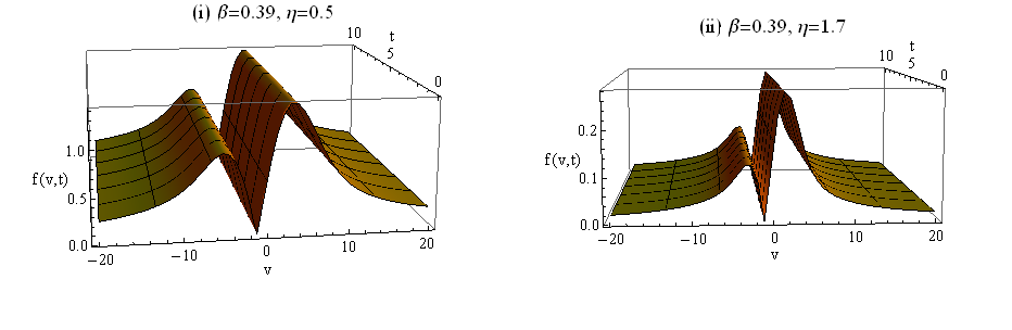
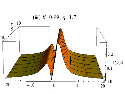
Figure 1: The behavior of distribution function, when (i) $B_{0}=1.5,\ c_{0}=2,\ n=10,\ \eta=1.7,\ A_{0}=1.3,\ A_{1}=2.3,\ B=5,\ m=2.5,\ \tau=t^{\beta},\ \beta=0.39,\ A_{2}=3,\ \mu=-0.5,\ B_{1}=1.9,\ B_{2}=0.7$. (ii) the same caption as in (i) but $\eta=1.7.$  (iii) the same caption as in (i) but  $\beta=0.99.$

Figures 1 show that the distribution function is mixed-Gaussian’s and that the friction coefficient plays a significant role in lowering the magnitude of the distribution density function. While the effect of vanning the fractional order plays a in lowering the tails.

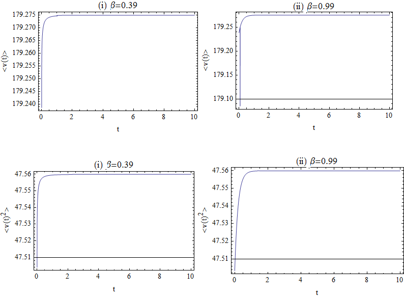
Figure 2: The mean and mean square of the velocity, when $B_{0}=1.5,\ c_{0}=2,\ n=10,\ \eta=0.5,\ A_{0}=1.3,\ A_{1}=2.3,\ B=5,\ m:=2.5,\ \tau=t^{\beta},\ \beta=0.99,\ A_{2}=3,\ \mu=-0.5,\ B_{1}=1.9,\ B_{2}=0.7.$

The order of the fractional time derivative has no remarkable effect on the mean and the mean square.

For the solution of fractional FPE in the caputo sense, the results in subsection 5.1 are displayed against $v$ and $t$, and they are shown in Figures3 (i)-(iii), for different values of $\alpha$ and the friction coefficient  $\eta$.

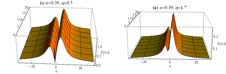
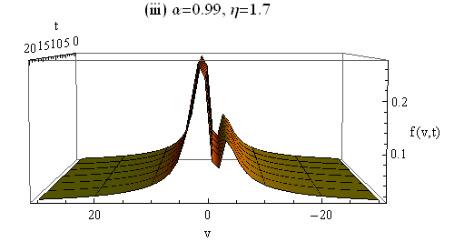
Figure 3: The behavior of distribution function, when (i) $B_{0}=1.5,\ c_{0}=2,\ n=10,\ \eta=0.5,\ A_{0}:=1.3,\ A_{1}=2.3,\ B=5,\ m=2.5,\ \tau=\frac{\Gamma(2-\alpha)}{\alpha}(T_{0}^{\alpha}-(T_{0}-t)^{\alpha}),\ \ \alpha=0.39,\ T_{0}=20,\ A_{2}:=3,\ \mu=-0.5,\ B_{1}:=1.9,\ B_{2}:=0.7.$ (ii) the same caption as in (i) but $\eta=1.7.$  (iiii) the same caption as in (i) but $\alpha=0.99.$

Figures 3 show mixed Gaussian’s. The friction coefficient plays a dominant role in lowering the magnitude of the distribution function. While when $\alpha=0.99$, permutation the Gaussian’s occurs.

Figures 4 show the mean and mean square of the velocity are displayed against t, by varying the fractional order.

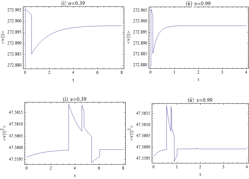
Figure 4: The mean and mean square for the same caption as in Figs.3.

Figures 4 (i) and (ii), show no remarkable variation in the mean and mean square when varying the fractional order.

5 Conclusions

An approach for finding solutions of linear PDEs with variable coefficients is presented. It is established by transforming the PDE to a system of first order PDEs and the extended unified method is implemented a class of solutions of fractional Fokker Planck equations are obtained. The solutions show that the distribution function is mixed-Gaussian’s. Further the friction coefficient plays the role of lowering the magnitude of the distribution function. On the other hand, varying the order of the fractional time derivative has the effect of permuting the Gaussian’s the distribution function.

References

• [11] R. Kazakeviˇcius, J. Ruseckas, Anomalous diffusion in non homogeneous media: power spectral density of signals generated by time-subordinated nonlinear Langevin equations. Physica A 438, 210–222 (2015).
• [2] A. Compte, Continuous time random walks on moving fluids. Phys. Rev. E 55(6), 6821 (1997).
• [3] V. Uchaikin, Anomalous transport equations and their application to fractal walking. Physica A 255, 65–92 (1998).
• [4] R. Klages, G. Radons, L. M. Sokolov, Anomalous transport: foundations and applications.Wiley, New York (2008)
• [5] I. Goychuk, Fractional-time random walk sub diffusion and anomalous transport with finite mean residence times: faster, not slower. Phys. Rev. E 86(2), 021113 (2012).
• [6] J. Anderson, E. Kim, S. Moradi, A fractional Fokker-Planck model for anomalous diffusion. Phys. Plasma 21(12), 122109 (2014).
• [7] M. Caputo , M. Fabrizio , A new definition of fractional derivative without singular Kernel, Progr. Fract. Differ. Appl. 1, 73–85 (2015).
• [8] J. Losada , .J. Nieto, Properties of the new fractional derivative without singular Kernel, Progr. Fract. Differ. Appl. 1, 87–92 (2015).
• [9] A. Atangana, D. Baleanu, New fractional derivatives with non-local and non-singular kernel: theory and applications to heat transfer model Therm Sci, 20 (2016) 763-769.
• [10] A. M. Tawfik, H. A. Fichtner, A. Elhanbaly , Schlickeiser R, An analytical study of fractional Klein–Kramers Approximations for describing anomalous diffusion of energetic particles.,J. of Stat. Phys. 174,830–845 (2019).
• [11] S. Moradi, J. Anderson, B. Weyssow, A theory of non-local linear drift wave transport. Phys. Plasmas 18(6), 062106 (2011).
• [12] E. Barkai, Stable equilibrium based on Lévy statistics: stochastic collision models approach. Phys. Rev. E 68(5), 055104 (2003).
• [13] S. Moradi, J. Anderson, Non-local gyrokinetic model of linear ion-temperature-gradient modes. Phys. Plasmas 19(8), 082307 (2012).
• [14] H. Risken, The Fokker-Planck Equation. Springer Series in Synergetics, vol. 18. Springer, Berlin (1989).
• [15] N. G. Van Kampen, Stochastic processes in chemistry and physics. Amsterdam 1, 120–127 (1981).
• [16] W. Chen, Timespace fabric underlying anomalous diffusion, Chaos, Solitons and Fractals 28, 923929 (2006).
• [17] W. Chen, Fractional and fractal derivatives modeling of turbulence [J], Arxiv preprint nlin/0511066, (2005).
• [18] R. Kanno, Representation of random walk in fractal space-time, Physica A 248, 165175 (1998) .
• [19] F. A. Al-Musallam, and V. K. Tuan,"H-Function with Complex Parameters II: Evaluation." Int. J. Math. Math. Sci. b25, 727-743, (2001).
• [20] M.I.Syama , M. Al -Refa, Fractional differential equations with Atangana–Baleanu fractional derivative: analysis and applications.Chaos, Solitons & Fractals 2, 100013 (2019).
• [21] I. Podlubny, Fractional Differential Equations: An Introduction to Fractional Derivatives, Fractional Differential Equations, toMethods of Their Solution and Some of Their Applications, vol. 198. Academic Press, Cambridge (1998)
• [22] H. I. Abdel-Gawad , M. Tantawy, D. Baleanu, Fractional KdV and Boussenisq-Burger’s equations, reduction to PDE and stability approaches. Math. Meth. Appl. Sci. on line.(2020)
• [23] N.H Sweilam, S. M. ALMekhlafi, D Baleanu, Optimal Control for a Fractional Tuberculosis Infection Model Including the Impact of Diabetes and Resistant Strains J.of Adv. Res. 17, 125–137 (2019)
• [24] N. H. Sweilam, S. M Ahmed, M Adel, A simple numerical method for two-dimensional nonlinear fractional anomalous sub-diffusion equations, Math Meth Appl. Sci. ;1–20 (2020).
• [25] H.. I. Abdel-Gawad, Towards a unified method for exact Solutions of evolution Equations. An application to reaction diffusion equations with finite memory transport, J. Stat. Phys. 147, 506–521 (2012).
• [26] H. I. Abdel-Gawad, , N El-Azab, and M. Osman, Exact solution of the space-dependent KdV equation by the extended unified method, JPSP, 82,044004,(2013).
• [27] H. M. Srivastava , H. I. Abdel-Gawad and Khaled M. Saad, Stability of Traveling Waves Based upon the Evans Function and Legendre Polynomials, Appl. Sci. 10, 846 (2020).
• [28] H. .I. Abdel-Gawad , M. Tantawy and R. E. Abo-Elkhair, On the extension of solutions of the real to complex KdV equation and a mechanism for the construction of rogue waves, Wave Random Complex. 26, 397–406 (2016).
• [29] D. Kumar , J. Singh , D. Baleanu , M.A. Qurashi, Analysis of logistic equation pertaining to a new fractional derivative with non- singular kernel, Adv. Mech. Eng. 9 (1), 1–8 (2017).
• [30] A. Atangana , B.T. Alkahtani , Analysis of non- homogeneous heat model with new trend of derivative with fractional order, Chaos Soliton Fract. 89, 566–571 (2016).
• [31] A. Choudhary , D. Kumar, J. Singh, Analytical Solution of fractional differential equations arising in fluid mechanics by using Sumudu transform method, Nonl. Eng. 3 (3), 133–139 (2014) .
• [32] J.-S. Duan, R. Rach, D. Baleanu, A. M. Wazwaz, A review of the Adomian decomposition method and its applications to fractional differential equations., Commun. Frac. Calc. 73 - 99 (2012).
• [33] M. Magdziarz and A. Weron, Numerical approach to the fractional Klein-Kramer’s equation , Phys. Rev. 76, 066708 (2007).
• [34] K. Sau Fa, Generalized Klein-Kramer’s equations, J. Chem. Phys. 137, 234102 (2012).