Investigating the Chinese Postman Problem on a Quantum Annealer

Abstract

The recent availability of quantum annealers has fueled a new area of information technology where such devices are applied to address practically motivated and computationally difficult problems with hardware that exploits quantum mechanical phenomena. D-Wave annealers are promising platforms to solve these problems in the form of quadratic unconstrained binary optimization. Here we provide a formulation of the Chinese postman problem that can be used as a tool for probing the local connectivity of graphs and networks. We treat the problem classically with a tabu algorithm and simulated annealing, and using a D-Wave device. The efficiency of quantum annealing with respect to the simulated annealing has been demonstrated using the optimal time to solution metric. We systematically analyze computational parameters associated with the specific hardware. Our results clarify how the interplay between the embedding due to limited connectivity of the Chimera graph, the definition of logical qubits, and the role of spin-reversal controls the probability of reaching the expected solution.

1 Introduction

Since their proposal by Kadowaki and Nishimori Kadowaki_PhysRevE1998 , quantum annealers (such as D-Wave machines) have advanced to the point that there is now a community of users whose goal is mainly to apply adiabatic quantum optimization (AQO) to a diverse set of computational problems in fields ranging from materials venturelli2015quantum and biological properties DiFelice ; perdomo2012finding to machine learning li2019unconventional ; neven2008image , fault detection faultdetection_ICT2016 and optimization Neukart ; Bian_2019 ; Stollenwerk_IEEE2020 ; SHOWALTER2014395 ; 8656874 ; Gomes2016OptimizationOR . Adiabatic quantum computation has been extensively reviewed albash2018adiabatic ; Das_RevModPhys2008 ; mcgeoch_book2014 ; aharonov2008adiabatic , as well as hardware/software aspects of D-Wave quantum annealers Dwave_Nature2011 ; Raymond_ICT2016 ; HardwareDWave_IEEE2014 ; boixo2014evidence ; albash2015reexamining . However, it remains important to expand the library of applications of quantum annealing for several reasons. First, these problems are stepping stones on the way to solving practical problems that may be beyond the reach of classical computation. Further, by comparing these algorithms with their classical counterparts one can probe the computational reach of quantum devices. Lastly, they enable both the providers and the users to identify optimal modes of operation and necessary improvements for the currently available machines.

AQO proceeds from an initial Hamiltonian $H_{0}$ to a final Hamiltonian $H_{1}$ whose ground state encodes the solution of the computational problem under consideration Santoro_Science2002 . The evolution is controlled by $t\in[0,T]$ (possibly with $T\rightarrow\infty$) through two monotonic functions $A(t)$ and $B(t)$ such as $A(T)=0$ and $B(0)=0$:

$$H(t)=A(t)H_{0}+B(t)H_{1}.$$

Starting from the ground state of $H_{0}$, the adiabatic theorem guarantees that the quantum state will remain in the ground state of $H(t)$, under Schrödinger evolution, provided that the Hamiltonian is varied slowly enough Kadowaki_PhysRevE1998 . In D-Wave systems, the initial configuration is given by the ground state of $H_{0}=-\sum_{i}h_{i}\sigma^{x}_{i}$ ($\sigma^{\alpha}_{i}$ are the Pauli operators for spin $i$ in the direction $\alpha$) with all the spins aligned along the $x$-direction. During the adiabatic process those spins start to interact à la Ising,

$$H_{1}=\sum_{ik}J_{ik}\sigma^{z}_{i}\sigma^{z}_{k}+\sum_{i}h_{i}\sigma^{z}_{i},$$

according to the specific choice of the parameters $J_{ik}$ and $h_{i}$. Since $[H_{0},H_{1}]\neq 0$, the quantum evolution is not trivial. At the end of each adiabatic cycle, a reading of the spin configuration in the $z$-basis provides a classical sample with a specific energy ($[\sigma^{z}_{i},H_{1}]=0$). Repeated measurements allow to extract the probability distribution for the solution. AQO mimics classical simulated thermal annealing but uses quantum superposition and tunneling instead of thermal fluctuations in order to reach a global minimum Denchev_PhysRevX2016 . While D-Wave has been successfully applied to solve many difficult problems, the advantages of D-Wave system to analyze optimization problems over classical algorithms are not clear; noise and decoherence play an important role and performance depends on parameters that are not easily controllable mishra2018 ; Tameem_PhysRevX2018 ; parekh2016benchmarking ; karimi2012investigating .

In this paper, we use D-Wave to analyze the undirected Chinese postman problem (CPP) Garey originally formulated in 1962 by the mathematician Kwan Mei-ko CPP . The CPP involves finding the “length” of the shortest closed path traveling across all edges of the network at least once. From a practical point of view the CPP problem is of interest in many situations where something or someone has to periodically traverse or inspect every link in a network, e.g. parallel programming, security patrolling, school bus route, etc. Modifications of routing problems may be used to model defects and transport in solids, which motivates us to choose CPP problem for the exploration of quantum computation in materials science. Besides all the possible applications, it is worthy to underline that none of the problems in the CPP class has been yet solved on a quantum annealer. The idea of this work is to implement the easiest CPP problem as a starting point towards developing generalizations to more complicated situations. There are several algorithms that solve the CPP Pearn ; Ahr ; Zhang ; Eiselt . This paper introduces a quadratic unconstrained binary optimization (QUBO) formulation of the CPP, which can be programmed into a quantum annealer. In addition, we run our algorithm on D-Wave 2X, detail the parameters that control the quality of the results, and exploit the solutions to probe features of the network topology.

Figure 1: Left panel: The network $G(E,V,w)$ used to illustrate the solution of the CPP. Right panel: One possible solution path of the CPP in this specific network.

2 The Chinese Postman Problem

The CPP is modeled using a network $G(V,E,w)$ (with $V=\{v_{1},v_{2},\dots\}$ being the set of all the nodes, $E=\{(v_{1},v_{2}),\dots,(v_{i},v_{j}),\dots\}\subset V\times V$ the set of all the edges, and $w:E\rightarrow\mathbb{R}$ a mapping assigning a “length” $w_{ij}$ to each edge). The goal is to find the shortest closed path length that crosses all the elements of $E$ at least once. While the undirected CPP and the directed CPP can be solved in polynomial time, common generalizations (e.g. the mixed CPP and the rural CPP) are NP-hard CPPApplications_2005 . The CPP admits a solution if and only if there exists at least one Eulerian cycle, i.e. a cycle that crosses each edge exactly once Euler ; Hedetniemi . A finite graph contains zero odd degree nodes (Eulerian graph) or an even number (non-Eulerian graph). In case of non-Eulerian network topologies, the algorithm dictates that extra paths linking odd degree nodes must be added to guarantee the existence of an Eulerian cycle; in other words the algorithm allows for the edges to be crossed more than once. Then, the shortest extra path has to be chosen. The two cases above are solved exactly.
In the network of Fig. 1a, for instance, there are four nodes of odd degree, $V_{O}=\{v_{0},v_{1},v_{2},v_{3}\}\subset V$ ($|V_{O}|=d=4$) and three possibilities for the extra paths

$$\begin{split}m(\pi_{1})=\quad&W(v_{0},v_{1})+W(v_{2},v_{3})=2+3=5\\ m(\pi_{2})=\quad&W(v_{0},v_{2})+W(v_{1},v_{3})=5+5=10\\ m(\pi_{3})=\quad&W(v_{0},v_{3})+W(v_{1},v_{2})=7+7=14.\end{split}$$ (1)

The “length” of each extra path between pairs of odd degree nodes is determined by computing the minimum across all the possible paths in $G(V,E,w)$ , e.g. $W(v_{0},v_{3}$) is the minimum between $w(v_{0},v_{1})+w(v_{1},v_{3})=7$, $w(v_{0},v_{2})+w(v_{2},v_{3})=11$, $w(v_{0},v_{5})+w(v_{5},v_{1})+(v_{1},v_{3})=9$, etc. The shortest “length”, which is the solution of the CPP problem, is given by the sum of all the arcs’ lengths plus the shortest extra path,

$$l_{T}(G)=\sum_{e\in E}w(e)+W(v_{0},v_{1})+W(v_{2},v_{3})=25+5.$$

The path corresponding to the solution of the CPP is shown Fig. 1b. Note that the path is not unique; at least a second path exists by the inversion of all the edge directions (since we are dealing with an undirected CPP).

Goodman and Hedetniem Goodman demonstrated that given a finite undirected network $G(V,E,w)$ with $d$ odd degree nodes, it is always possible (1) to find $(d-1)!!$ perfect matchings $\pi_{\alpha}$ of pairs of odd degree nodes (as in Eq. 1), (2) to assign to each $\pi_{\alpha}$ a minimal path “length” $m(\pi_{\alpha})$, and (3) to determine the solution of the CPP by using

$$l_{T}(G)=\sum_{e\in E}w(e)+\min_{\alpha}m(\pi_{\alpha})=\sum_{e\in E}w(e)+M_{min}$$ (2)

3 QUBO for the CPP

In quantum annealing, optimization problems are encoded as Ising Hamiltonians whose ground state configuration is a binary string solution to the corresponding problem. Ising Hamiltonian can be mapped to quadratic unconstrained binary optimization (QUBO). Finding the ground state of the Ising then is equivalent to the minimization of a quadratic form in $\mathbb{Z}_{2}^{2N}$ Laughhunn .

Here, we are going to derive for the first time the QUBO formulation for the CPP problem. In order to do that, the objective function $m(\pi_{\alpha})$ has to be expressed as binary integer problem (BIP, for a binary variable, $x=x^{2}$). Given an undirected network $G(V,E,w)$ and $V_{O}\subset V$ with $d$ nodes of odd degree, the possible paths can be represented by the variable $x_{ij}$ where $i,j\in\{0,..,d-1\}$ and $i\neq j$ such as:

$$x_{ij}=\begin{cases}1\quad\text{if node}\,i\,\text{is paired with node}\,j\\ 0\quad\text{otherwise.}\end{cases}$$ (3)

Thus, a binary vector $\mathbf{x}\in\mathbb{Z}_{2}^{d(d-1)}$ of decision variables for the QUBO can be used to search for the global shortest “length” by minimizing the sum of all the shortest distances of all the permutations of nodes of odd degree.

$$F(\mathbf{x})=\sum_{i\neq j}^{d-1}W_{ij}x_{ij},$$ (4)

where $W_{ij}=W(v_{i},v_{j})$ is the “length” of the minimum path between the odd degree nodes $i$ and $j$ by taking into account all the network features as discussed in Sec. 2. In the case of the CPP, $F(\mathbf{x})$ is subject to two constrains which guarantee that the ordered pairs of nodes are unique and that each node is counted only once in each subset $\pi_{\alpha}$. $P_{1}(\mathbf{x})$ penalizes double counting of pairs of nodes in $V_{O}$ and $P_{2}(\mathbf{x})$ penalizes whenever the combination of the pairs is not legal (see the Supplementary Material for details). Overall, the quadratic function to be optimized is

$$Q(\mathbf{x})=\sum_{i\neq j}^{d-1}W_{ij}x_{ij}^{2}+pP_{1}(\mathbf{x})+pP_{2}(\mathbf{x})$$ (5)

with

$$P_{1}(\mathbf{x})=\sum_{i\neq j}^{d-1}\left(1-\sum_{j=0}^{d-1}(x_{ij}+x_{ji})\right)^{2}$$ (6)

and

$$P_{2}(\mathbf{x})=\sum_{i\neq k;j\neq k}^{d-1}(x_{ik}x_{jk}+x_{ki}x_{kj})$$ (7)

for some constant $p\geqslant d$.

For the network shown in Fig. 1 all the ordered pair of vertices of odd degree can be easily listed:

$$\begin{split}&\{(v_{0},v_{1}),(v_{0},v_{2}),(v_{0},v_{3}),(v_{1},v_{0}),(v_{1},v_{2}),(v_{1},v_{3}),\\ &(v_{2},v_{0}),(v_{2},v_{1}),(v_{2},v_{3}),(v_{3},v_{0}),(v_{3},v_{1}),(v_{3},v_{2})\}\end{split}$$

and the representing vector is $\mathbf{x}=(x_{01},x_{02},x_{03},x_{10},x_{12},x_{13},x_{20},x_{21},x_{23},x_{30},x_{31},x_{32})\in\mathbb{Z}_{2}^{12}$. The legal combinations of pairs are represented by $\pi_{\alpha}$ with $\alpha=1,2,3$. The coefficients of the matrix representing the quadratic form are determined using $p=8$ and are shown in Table 1. The minimum of $Q(\mathbf{x})$ is given by

$$\mathbf{x_{*}}=(1,0,0,0,0,0,0,0,1,0,0,0),$$

meaning that the legal partition of pairs formed with odd degree nodes is $\{(v_{0},v_{1}),(v_{2},v_{3})\}$. The shortest paths are shown in Fig. 1b. The minimum sum of pairs of nodes with odd degree is given by $Q(\mathbf{x_{*}})$.

Pairs	$x_{01}$	$x_{02}$	$x_{03}$	$x_{10}$	$x_{12}$	$x_{13}$	$x_{20}$	$x_{21}$	$x_{23}$	$x_{30}$	$x_{31}$	$x_{32}$
$x_{01}$	-12	16	16	48	16	16	16	16	0	16	16	0
$x_{02}$	16	-6	16	16	16	0	48	16	16	16	0	16
$x_{03}$	16	16	-2	16	0	16	16	0	16	48	16	16
$x_{10}$	48	16	16	-12	16	16	16	16	0	16	16	0
$x_{12}$	16	16	0	16	-2	16	16	48	16	0	16	16
$x_{13}$	16	0	16	16	16	-6	0	16	16	16	48	16
$x_{20}$	16	48	16	16	16	0	-6	16	16	16	0	16
$x_{21}$	16	16	0	16	48	16	16	-2	16	0	16	16
$x_{23}$	0	16	16	0	16	16	16	16	-10	16	16	48
$x_{30}$	16	16	48	16	0	16	16	0	16	-2	16	16
$x_{31}$	16	0	16	16	16	0	0	16	16	16	-6	16
$x_{32}$	0	16	16	0	16	16	16	16	48	16	16	-10

Table 1: QUBO matrix for CPP on the network in Fig. 1. The penalty constant is chosen to be equal to the number of nodes+2 ($p=8$). Details on the derivation of the matrix elements $Q_{ij}$ can be found in the SM, Sec. 1.

4 Computational Methods

We first solve several cases of the CPP classically using the software qbsolv Qbsolv_new, a solver that finds the minimum value for QUBO problem using a metaheuristic tabu search algorithm Gendreau2003 . We then implement our formulation on D-Wave 2X following a protocol that facilitates comparisons with the classical solutions and provide insight on the parameters of the calculations. In order to estimate the efficiency of the quantum annealing we also compared with classical simulated annealing (SA) following the work of Albash and Lidar Tameem_PhysRevX2018 .

In D-Wave systems, physical qubits are arranged in a Chimera graph topology; in order to be able to represent the QUBO, a set of linked (logical) qubits must be defined S_Humble_2014 . Physical qubits are organized in chains to “simulate” the logical qubits; this is known as a minor embedding min_emb . D-Wave’s API provides a function called minorminer which heuristically searches for the optimal (minor)embedding Cai_2014 ; Choi2011 . minorminer minimizes the length of each embedding chain, as shorter chains are less prone to breaking into domains where physical qubits have opposite spin orientations. The choice of intra-chain coupling ($J_{F}$) is important as it affects the time-dependent energy spectrum in the adiabatic evolution and determines the ability of the chain to act as a single variable. $J_{F}$ couplings should be strong enough to avoid chain-breaking without dominating the dynamics. Tight bounds on these conditions are derived in Ref. Choi2011 . In addition, due to the dynamic range and the precision of the hardware control Barahona , the representation of the QUBO in terms of the Ising Hamiltonian parameters depends on the relative scale of $J_{ij}$ and $h_{i}$.

Our protocol on D-Wave involves: (1) selecting a network to study the CPP, (2) scaling appropriately the entries of the QUBO matrix, (3) embedding the specific QUBO topology on the Chimera graph using minorminer, (4) assessing the quality of different embeddings, (5) optimizing intra-chain coupling ($J_{F}$), (6) comparing the results with qbsolv when possible.

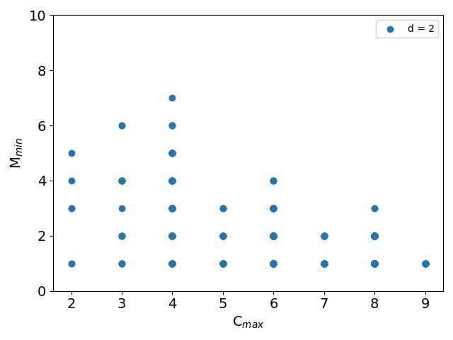
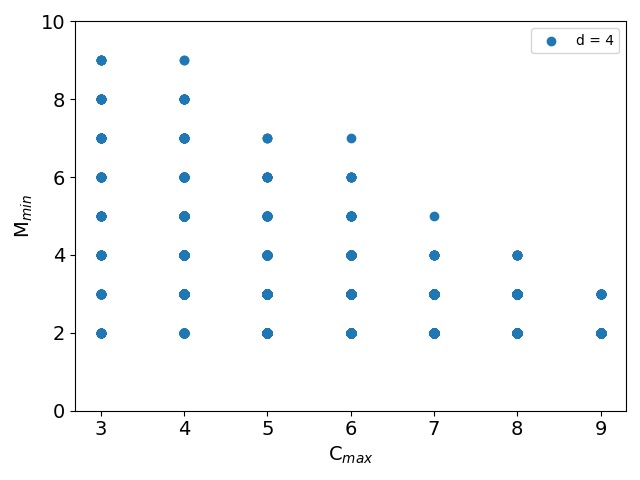
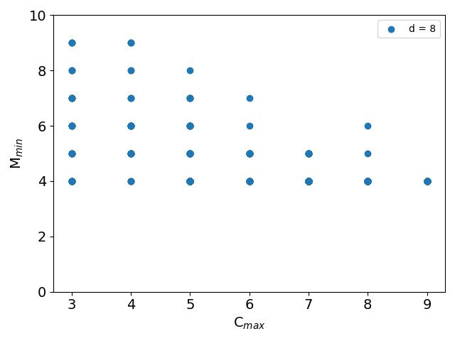
Figure 2: $M_{min}$ as a function of the largest degree of nodes in the graph (we used $w_{ij}=1\ \forall\ i,j$ to simplify the analysis). The results were obtained with a sample of 10,000 randomly generated graphs with $n=10$. Results are divided according to the number of nodes with odd degree ($d$) in the graph. We report only three representative subsets in this figure. Left panel: 875 graphs with $d=2$. Middle panel: 4,025 graphs with $d=4$. Right panel: 809 graphs with $d=8$.

5 Classical Results by qbsolv

In order to test the QUBO formulation and establish references for the D-Wave calculations, we randomly generate 10,000 non-Eulerian networks of order $n$ with variable number of nodes with odd degree $d\geqslant 2$ and variable size (the number of edges specified in $E\subset V\times V$).

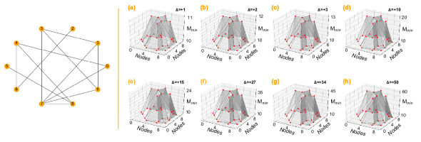
Figure 3: Left panel: Visual representation of the graph $G(E,V,w=1)$ with $n$=10 nodes and $d$=8. Right panel: value of $M_{min}(i,j)$ as function of the $(i,j)$ position of the defect in the adjacency matrix. Each plot corresponds to a different value ($\Delta$) for the defected edge.

As expected, longer CPP paths ($M_{min}$, see Eq. 2) are associated with the presence of nodes with small degree, conversely if there are large degree nodes, the value of $M_{min}$ is reduced to the minimum $M_{min}=d/2$. Notably, the result of the optimization problem depends on the degree of all the nodes in the network. In Fig.2, we report $M_{min}$ as function of the maximum degree ($c_{MAX}$) for graphs with $n=10$ where edge weights are all set to unity, $w_{ij}=\epsilon=1\ \forall\ i,j$. The CPP solution is sensible to the degree of the vertices suggesting that the CPP can be used to explore the degree of the nodes in a graph. In order to gain additional insight, we introduce multiple random “defects” in the network by varying one or more $w_{ij}$. In particular, we analyze $M_{min}$ in the case of $n=10,\,14,\,17$ (see Tab.2) by setting from one to threeedges to $\epsilon+\Delta$, with $\Delta=1,2,3,10,15,27,34,50$. Given a graph, the CPP has been solved for all the possible arrangements of one, two, and three defected edges in the graph. A total of 1,000 random graphs has been investigated with all the $\Delta$ values. Our intention is to explore ways to use the CPP algorithm to characterize defected networks.

$n$	$d$	$c_{MAX}$	$c_{min}$	$c_{1}$
10	8	3	1	2
14	4	5	1	2
17	4	8	2	0

Table 2: Main features of the graphs: number of vertices ($n$), number of nodes with odd degree ($d$), max degree ($c_{MAX}$) and min degree ($c_{min}$) among all nodes, number of nodes with degree equal to 1, ($c_{1}$).

For $n=10$, a reference graph with 8 nodes with odd degree that gives $M_{min}=10$ was chosen to illustrate the effect (see Fig. 3 left panel). The right panel of Fig. 3 shows the value of $M_{min}$ as function of the position of the defect in the $(i,j)$ element of the the adjacency matrix of the graph ($M_{min}(i,j)$). Due to the introduction of a single defect, 6 distinct peaks arise regardless the $\Delta$ value. Despite the difference in the absolute values of the maximum $M_{min}$ with $\Delta$, features and shapes are preserved. Since the adjacency matrix $A$ is, by definition, symmetric, only 3 distinct edges, $(v_{2},v_{6}),(v_{5},v_{8}),(v_{4},v_{6})$, are crucial for the CPP. Two different behaviors can be observed: (1) the edges $(v_{2},v_{6}),(v_{5},v_{8})$ link nodes with degree one ($v_{2}$ and $v_{5}$) or (2) $M_{min}$ is maximum for the edge $(v_{4},v_{6})$ is associated to a node of degree 2 ($v_{6}$). In general, $M_{min}$ reaches a maximum value when the postman is forced to travel twice of the edge with increased “length” (defect) when nodes with small degree are present. Similar behavior is observed in the case of two defects, while for three defects in a small graph is impossible to extract information regarding the local topology (nodes’ degree).

Finally, we analyze the case of networks with $n$=10, 14, 17 with random $w_{ij}$. One specific case of a network with $n=14$, $d=4$, and $c_{1}=2$ ($c_{1}$ is the number of vertices with degree equal to one) is shown in Fig. 4. In case of a large defect ($\Delta\gg w_{ij}\ \forall\ i,j$) the plots in Fig. 4 resemble the ones in Fig. 3. The edge weights take values in the range $w\in\{1,\dots,5\}$. For $\Delta\geqslant 27$ the $M_{min}$ representation (we used the same format as in Fig. 3) is equivalent to the one of the graph (Fig.4a). This is reasonable, if the defected edge is linked to one of the two nodes with degree one, it has to be included in the $M_{min}$ computation. Overall, for arbitrary networks assessing $M_{min}(i,j,\Delta)$ is an effective way to detect nodes of degree one. The appropriate $\Delta$ value required to access the local connectivity depends on $c_{MAX}$, $d$, and the size of the network.

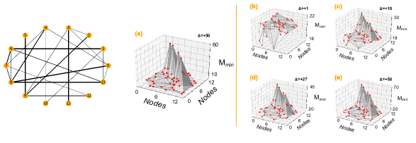
Figure 4: Left panel: Visual representation of the network $G(E,V,w)$ with order $n=14$, four odd degree nodes ($d=4$ $\{v_{1},v_{5},v_{8},v_{11}\}$: the weights $w_{ij}\in\{1,\dots,5\}$ are shown with line thickness. (a) $M_{min}(i,j)$ is represented as in Fig. 3 for $\Delta=0$. Right panel: Plots illustrate the effect of introducing defects of magnitude $\Delta$ on the edge $(v_{i},v_{j})\in E$.

6 Results by Quantum Annealing (D-Wave)

Using D-Wave 2X, we analyze the quality of the CPP solution by changing embedding parameters (see Sec. 4), the intra-chain coupling ($J_{F}$), and the scaling of the QUBO to fit the dynamic range of the hardware. Initially, we select graphs ($w_{ij}=1\ \forall i,j$) with increasing number of odd degree nodes ($d=2,4,6,8$, intuitively pointing to the complexity of the specific CPP), rescale the QUBO matrix elements (using autoscale), and embed the CPP problem on $12\times 12\times 8$ physical qubits (minus 54 malfunctioning physical qubits) of the D-Wave Chimera. The “quality” of the embeddings is assessed using the probability of reaching the desired ground state (P_gs) and the performance of DWave 2X is assessed by computing the time to get the solution with probability 99%:

$$\mbox{T}_{99}=\dfrac{ln(1-0.99)}{ln(1-\mbox{P}_{gs})}T$$

where T is the annealing time. Even after selecting the embedding (see for instance Fig. 5 for the cases $d=4$ and $d=8$), the P_gs depends significantly on the choice of the intra-chain coupling $J_{F}$ venturelli2015quantum ; Stollenwerk_IEEE2020 and the annealing time T. Because the best T is different from one embedding to another, it is not possible to select a T that allows top performance for all the embeddings. According to this, we have evaluated $\mbox{T}_{99}$ using the default T=$20\mu s$ ($\mbox{T}^{A}_{99}$) and the optimal annealing time for the best embedding at a given size $d$ of the problem ($\mbox{T}^{B}_{99}$). The performance of D-Wave 2X has been compared also with simulated annealing as implemented in D-Wave Ocean SDK Ocean . Following Albash and Lidar Tameem_PhysRevX2018 , the time to solution for SA reads as:

$$\mbox{TTS}=N^{2}\dfrac{ln(1-0.99)}{ln(1-\mbox{P}_{gs})}\tau_{s}n_{s}$$

where $N$ is the size of the graph (see Supporting Material for further clarifications), $n_{s}$ is the number of sweeps, and $\tau_{s}=1/f_{SA}$ the time required to perform a single sweep ($f_{SA}$ is the number of spin updates per unit time). Because the SA algorithm performs one spin flip per time step and the clock rate of our cpu is $2.4$ GHz, $f_{SA}=2\,\text{ns}^{-1}$. The chosen SA annealing schedule $\beta$ is comparable to the one of D-Wave 2X.

$d$	Logical qubits	Number of Qij terms	Physical qubits	Pgs (%)	T${}^{A}_{99}$ (s)	T${}^{B}_{99}$ (s)	TTS (s)
2	2	2	2	99.99	9.7e-6	7.1e-6	4.0e-4
4	12	54	44	87.83	4.37e-5	2.0e-5	7.0e-3
6	30	256	248	51.07	1.29e-4	2.3e-4	1.8e-2
8	56	700	864	0.21	4.38e-2	1.8e-2	7.9e-2

Table 3: Parameters and performance of the “optimal” embedding for the CPP cases studied with D-Wave 2X: number of nodes with odd degree ($d$), number of logical qubits (equal to the number of variables in the optimization problem), number of terms in the QUBO, number of physical qubits required in the embedding, best probability of finding the correct ground state P_gs, time to solution with T=20 $\mu s$ (T${}^{A}_{99}$), optimal time to solution T (T${}^{B}_{99}$), time to solution of the simulated annealing TTS. The embeddings were generated with minorminer and chosen according to the criteria discussed in the text.

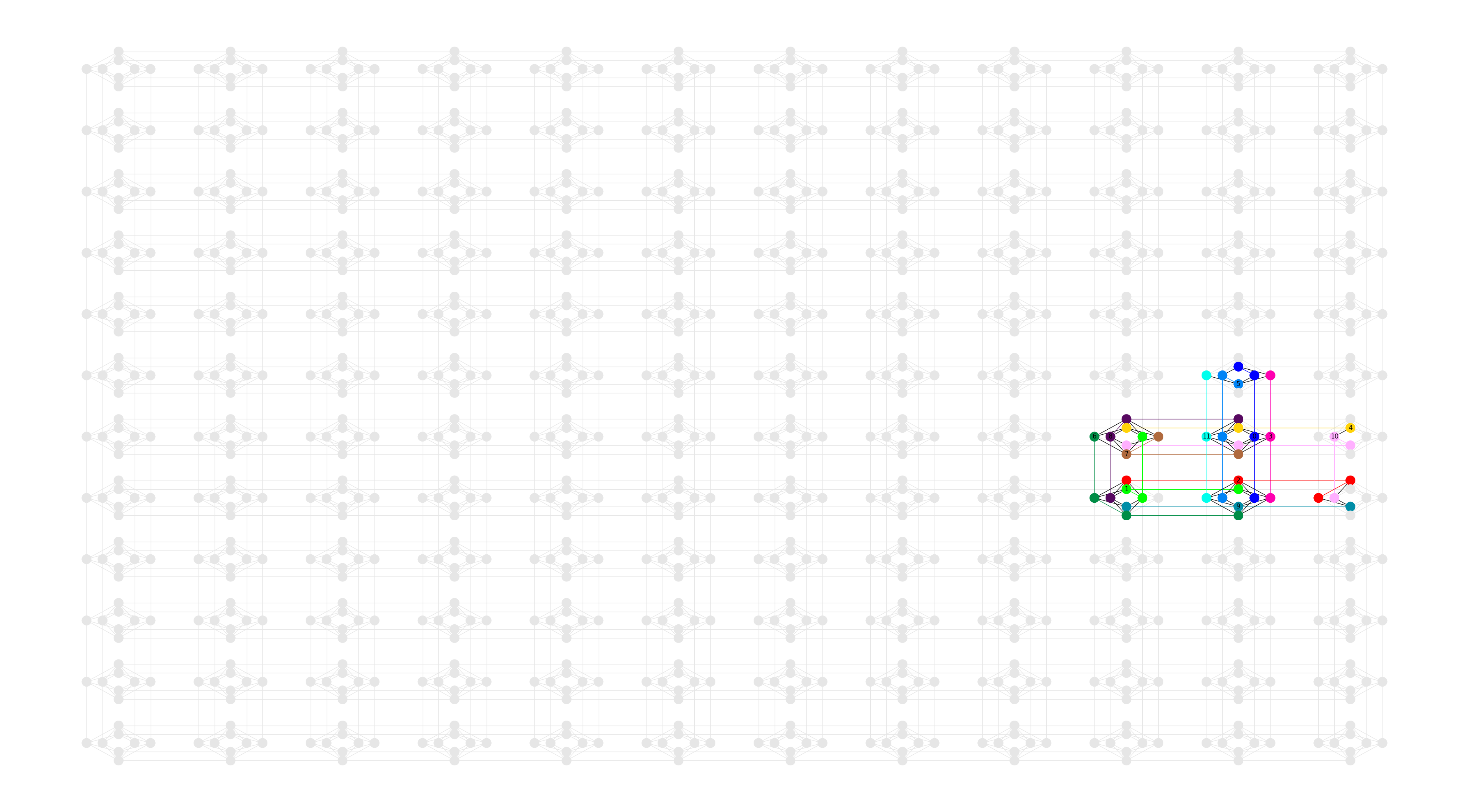
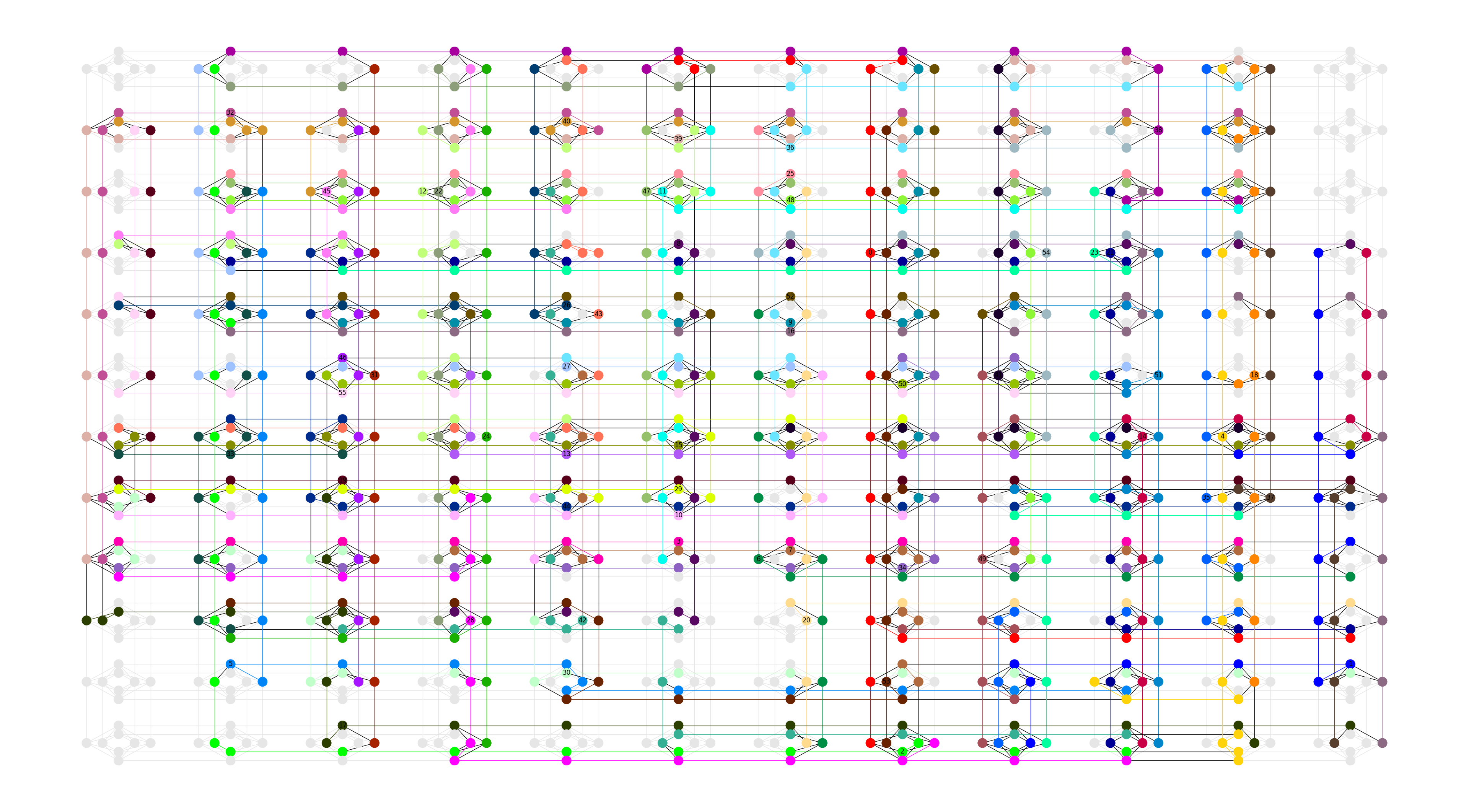
Figure 5: Map of two of the “optimal” embeddings on the whole Chimera graph for case of a QUBO with $d=4$ (left) and $d=8$ (right). Different colors highlight different spin-chains, namely different logical qubits. The case for $d=8$ has long chains and uses 902 out of 12 $\times$ 12 $\times$ 8 physical qubits in D-Wave 2X. This makes very difficult to control the noise induced by chain breaking.

Tab. 3 reports the information for the “optimal” embeddings (largest P_gs) for each problem size ($d$) we considered. For $d=2$ physical and logical qubits are the same so the D-Wave results match the classical results consistently (P_gs=99.97%, see Tab. 3). However, for $d\geqslant 4$, embeddings become necessary. When the chain alignment in an embedding breaks, D-Wave automatically performs a majority vote to assign a value to the corresponding logical qubit: we report in the Supplementary Material (SM Tab. 1) detailed information on the topology of the embeddings as well as P_gs and the best time to solution (T₉₉) counting all chains regardless possible loss of intra-chain alignment. Here we only consider the solution without broken chains, and do not perform any post-processing of the D-Wave solutions.

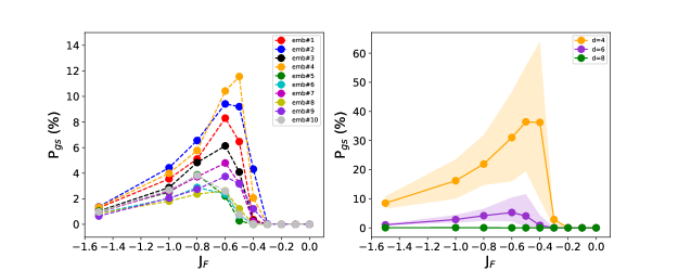
Figure 6: Probability of finding the correct ground state (P_gs) on the D-Wave 2X defined as the ratio between the number of correct solutions and total annealing cycles (40000) as a function of the intra-chain ferromagnetic coupling J_F given in units of the largest coefficient of the embedded Ising model. Only solutions with unbroken chains are counted. Runs are performed using 100 spin reversal operations. Left Panel: We report the case of $d=6$ where different embeddings (different colors) computed with minorminer have been considered. Right panel: Average P_gs (solid lines) computed for different problem size $d$. The average is taken over 10 embeddings per problem size. The shaded areas highlight the variation between the lowest and the highest P_gs among the considered embeddings.

Fig. 6 shows the combined effect of $J_{F}$ and of specific embeddings on P_gs for networks with different dimensions ($d=4,6,8$). For $d=6$, the maximum P_gs (left panel) is greatly affected both by the choice of the embedding and the optimal $J_{F}$; that is true for all the considered embeddings. The classical result is matched in 11.6% of 40,000 annealing cycles. The result for $d=4$ (right panel and Supplementary Material) are similar in term of $J_{F}$ but the P_gs reaches 60%. For $d=8$, the optimal $J_{F}$ is close to 1.0, however, the $J_{F}$ optimization does not improve significantly the performance in this case. Indeed, chains are very long ($\geqslant 23$), intra-chain alignment is lost (chain breaking fraction close to one), and the classical solution is practically never reached (0.1%). We observe that the choice of an optimal $J_{F}$ improves the performance and generally depends on the size of the problem. Overall, the choice of the embedding greatly affects the chance of getting a finite value for P_gs (see Supplementary Material).
The performance in terms of T${}^{A}_{99}$ are shown in Fig. 7 for different sizes of the problem ($d$). As Albash and Lidar have shown before Tameem_PhysRevX2018 , when D-Wave parameters are not optimized (in their case anneal time), the inferred scaling of the time to solution can be lower than the actual scaling. Not optimizing the embedding will have the same effect because T₉₉ can change substantially under different embeddings. How to find an optimal embedding remains an important open question.
The solutions accuracy is also influenced by the number of spin reversal (SR) operations which are performed to limit the effect of persistent bias on the physical couplers. The observed values for P_gs in the absence of spin reversals changes only modestly when we increase SR (see Supporting Material). For the data presented Fig. 6 and Fig. 7, we set the value to SR=100, as in this case it guarantees the convergence of the performance.

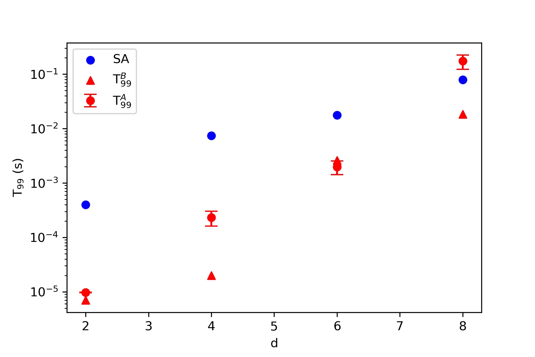
Figure 7: Average time to solution for the default annealing time T=20 $\mu s$ (T${}^{A}_{99}$, red dots) and the optimal annealing time for the best performing embedding (T${}^{B}_{99}$, red triangles), for different problem sizes ($d$=2,4,6,8). Data from 10 different embeddings are bootstrapped over 5000 random samples, and the error bars respond $\pm 2\sigma$ of the bootstrapped sample. In the $d=2$ case, only a single embedding is considered. The scaling of time to solution $T^{A}_{99}$ with the size $d$ is exponential with coefficients $\alpha_{A}=0.52\pm 0.12$. Blue dots correspond to data obtained with simulated annealing (SA) as implemented in Ocean Ocean .

7 Conclusions

We framed the Chinese postman problem (CPP) as a quadratic unconstrained binary optimization problem and solved it using qbsolv, classical simulated annealing, and D-Wave 2X. Further, we used the solution of the CPP to probe local properties of the graph topology. We devised a simple workflow and explored systematically the parameter setting on the quantum annealer, specifically the effect of embedding, intra-chain coupling $J_{F}$, spin-reversal, and problem complexity on the quality of the solutions obtained. By analyzing networks with increasing number of odd degree nodes ($d$), we observed the critical role of the embedding and the appropriate scaling of the qubits interactions, $J_{F}$. Namely, even in cases where the correct solution is hardly reachable under the default settings, one must tune these knobs to get the solutions and optimize the performance. The efficiency of the quantum annealing has been compared with classical simulated annealing in order to assess any possible quantum advantage, finding that quantum annealing as implemented in D-Wave 2X is on average an order of magnitude faster than classical simulated annealing on commercial traditional hardware. Although the CPP is solvable classically in polynomial time, generalizations such as the Mixed CPP or the Windy CPP are NP-hard problems which can take advantage from adiabatic quantum optimization. Such generalizations are potential extensions of this work.

References

- (1) T. Kadowaki, H. Nishimori, Phys. Rev. E 58, 5355 (1998). DOI 10.1103/PhysRevE.58.5355. URL https://link.aps.org/doi/10.1103/PhysRevE.58.5355
- (2) D. Venturelli, S. Mandra, S. Knysh, B. O’Gorman, R. Biswas, V. Smelyanskiy, Physical Review X 5(3), 031040 (2015)
- (3) R. Li, R. Di Felice, R. Rohs, D. Lidar, npj Quantum Information 4(1), 14 (2018). DOI 10.1038/s41534-018-0060-8
- (4) A. Perdomo-Ortiz, N. Dickson, M. Drew-Brook, G. Rose, A. Aspuru-Guzik, Scientific reports 2, 571 (2012)
- (5) R.Y. Li, S. Gujja, S.R. Bajaj, O.E. Gamel, N. Cilfone, J.R. Gulcher, D.A. Lidar, T.W. Chittenden, arXiv preprint arXiv:1909.06206 (2019)
- (6) H. Neven, G. Rose, W.G. Macready, arXiv preprint arXiv:0804.4457 (2008)
- (7) Z. Bian, F. Chudak, R.B. Israel, B. Lackey, W.G. Macready, A. Roy, Frontiers in ICT 3, 14 (2016). DOI 10.3389/fict.2016.00014. URL https://www.frontiersin.org/article/10.3389/fict.2016.00014
- (8) F. Neukart, G. Compostella, C. Seidel, D. von Dollen, S. Yarkoni, , B. Parney, Frontiers in ICT 4(29) (2017)
- (9) Z. Bian, F. Chudak, W. Macready, A. Roy, R. Sebastiani, S. Varotti, arXiv preprint arXiv:1811.02524 (2018)
- (10) T. Stollenwerk, B. O’Gorman, D. Venturelli, S. Mandrà, O. Rodionova, H. Ng, B. Sridhar, E.G. Rieffel, R. Biswas, IEEE Transactions on Intelligent Transportation Systems 21(1), 285 (2020). DOI 10.1109/TITS.2019.2891235
- (11) D.J. Showalter, J.T. Black, Acta Astronautica 105(2), 395 (2014). DOI https://doi.org/10.1016/j.actaastro.2014.09.013
- (12) A. Figueras, J.L. De La Rosa, S. Esteva, X. Cufí, in 2018 IEEE International Smart Cities Conference (ISC2) (2018), pp. 1–6
- (13) F.F. Gomes, M.C. Gomes, A.B. Gonçalves, in ICORES (2016)
- (14) T. Albash, D.A. Lidar, Reviews of Modern Physics 90(1), 015002 (2018). DOI 10.1103/RevModPhys.90.015002
- (15) A. Das, B.K. Chakrabarti, Rev. Mod. Phys. 80, 1061 (2008). DOI 10.1103/RevModPhys.80.1061. URL https://link.aps.org/doi/10.1103/RevModPhys.80.1061
- (16) C.C. McGeoch, Synthesis Lectures on Quantum Computing 5(2), 1 (2014)
- (17) D. Aharonov, W. Van Dam, J. Kempe, Z. Landau, S. Lloyd, O. Regev, SIAM review 50(4), 755 (2008)
- (18) M.W. Johnson, M.H. Amin, S. Gildert, T. Lanting, F. Hamze, N. Dickson, R. Harris, A.J. Berkley, J. Johansson, P. Bunyk, et al., Nature 473(7346), 194 (2011)
- (19) J. Raymond, S. Yarkoni, E. Andriyash, Frontiers in ICT 3, 23 (2016). DOI 10.3389/fict.2016.00023. URL https://www.frontiersin.org/article/10.3389/fict.2016.00023
- (20) P.I. Bunyk, E.M. Hoskinson, M.W. Johnson, E. Tolkacheva, F. Altomare, A.J. Berkley, R. Harris, J.P. Hilton, T. Lanting, A.J. Przybysz, J. Whittaker, IEEE Transactions on Applied Superconductivity 24(4), 1 (2014). DOI 10.1109/TASC.2014.2318294
- (21) S. Boixo, T.F. Rønnow, S.V. Isakov, Z. Wang, D. Wecker, D.A. Lidar, J.M. Martinis, M. Troyer, Nature physics 10(3), 218 (2014)
- (22) T. Albash, T.F. Rønnow, M. Troyer, D.A. Lidar, The European Physical Journal Special Topics 224(1), 111 (2015)
- (23) G.E. Santoro, R. Martoňák, E. Tosatti, R. Car, Science 295(5564), 2427 (2002). DOI 10.1126/science.1068774. URL https://science.sciencemag.org/content/295/5564/2427
- (24) V.S. Denchev, S. Boixo, S.V. Isakov, N. Ding, R. Babbush, V. Smelyanskiy, J. Martinis, H. Neven, Phys. Rev. X 6, 031015 (2016). DOI 10.1103/PhysRevX.6.031015. URL https://link.aps.org/doi/10.1103/PhysRevX.6.031015
- (25) A. Mishra, T. Albash, D.A. Lidar, Nature Communications 9(1), 2917 (2018). DOI https://doi.org/10.1038/s41467-018-05239-9
- (26) T. Albash, D.A. Lidar, Phys. Rev. X 8, 031016 (2018). DOI 10.1103/PhysRevX.8.031016. URL https://link.aps.org/doi/10.1103/PhysRevX.8.031016
- (27) O. Parekh, J. Wendt, L. Shulenburger, A. Landahl, J. Moussa, J. Aidun, arXiv preprint arXiv:1604.00319 (2016)
- (28) K. Karimi, N.G. Dickson, F. Hamze, M.H. Amin, M. Drew-Brook, F.A. Chudak, P.I. Bunyk, W.G. Macready, G. Rose, Quantum Information Processing 11(1), 77 (2012)
- (29) M. Garey, D. Johnson, Computers and Intractability: A Guide to the Theory of NP-Completeness (San Francisco: Freeman, 1978)
- (30) K. Mei-Ko, Chinese Mathematics 1 p. 273–277 (1962)
- (31) W.L. Pearn, C. Liu, Computers & Operations Research 22(5), 479 (1995). DOI 10.1016/0305-0548(94)00036-8
- (32) D. Ahr, G. Reinelt, Computers & Operations Research 33(12), 3403 (2006). DOI 10.1016/j.cor.2005.02.011
- (33) B. Zhang, J. Peng, Industrial Engineering and Management Systems 1(11), 18–25 (2012). DOI 10.7232/iems.2012.11.1.018
- (34) H. Eiselt, M. Gendreau, , G. Laporte, Operations Research 43(2), 231 (1995)
- (35) A.A. Assad, B.L. Golden, in Network Routing, Handbooks in Operations Research and Management Science, vol. 8 (Elsevier, 1995), pp. 375 – 483. DOI https://doi.org/10.1016/S0927-0507(05)80109-4. URL http://www.sciencedirect.com/science/article/pii/S0927050705801094
- (36) L. Euler, Commentarii Academiae Petropolitanae 8, 128–140 (1736)
- (37) S. Hedetniemi, Naval Research Logistics Quarterly 15(3), 453 (1968). DOI 10.1002/nav.3800150309
- (38) S. Goodman, S. Hedetniemi, SIAM Journal on Computing 2(1), 16 (1973). DOI 10.1137/0202003
- (39) D.J. Laughhunn, Operations Research 18(3), 454 (1970). DOI 10.1287/opre.18.3.454
- (40) M. Gendreau, An Introduction to Tabu Search (Springer US, 2003), pp. 37–54. DOI 10.1007/0-306-48056-5
- (41) T.S. Humble, A.J. McCaskey, R.S. Bennink, J.J. Billings, E.F. D’Azevedo, B.D. Sullivan, C.F. Klymko, H. Seddiqi, Computational Science & Discovery 7(1), 015006 (2014). DOI 10.1088/1749-4680/7/1/015006
- (42) S. Okada, M. Ohzeki, M. Terabe, S. Taguchi, Scientific Reports 9(1), 2045 (2019). DOI 10.1038/s41598-018-38388-4
- (43) J. Cai, W.J. Macready, A. Roy, arXiv preprint arXiv:1406.2741 (2014)
- (44) V. Choi, Quantum Information Processing 10(3), 343 (2011). DOI 10.1007/s11128-010-0200-3
- (45) F. Barahona, Journal of Physics A: Mathematical and General 15(10), 3241 (1982). DOI 10.1088/0305-4470/15/10/028
- (46) D-Wave Systems Inc 2018. https://github.com/dwavesystems/dwave-ocean-sdk