Radiative capture rates at deep defects from electronic structure calculations

Abstract

We present a methodology to calculate radiative carrier capture coefficients at deep defects in semiconductors and insulators from first principles. Electronic structure and lattice relaxations are accurately described with hybrid density functional theory. Calculations of capture coefficients provide an additional validation of the accuracy of these functionals in dealing with localized defect states. We also discuss the validity of the Condon approximation, showing that even in the event of large lattice relaxations the approximation is accurate. We test the method on GaAs:$V_{\text{Ga}}$-$\text{Te}_{\text{As}}$ and GaN:C${}_{\text{N}}$, for which reliable experiments are available, and demonstrate very good agreement with measured capture coefficients.

I Introduction

Optical techniques such as absorption, photoluminescence (PL), PL excitation spectroscopy, and time-dependent PL are powerful tools for studying defects in semiconductors and insulators Davies (1999). However, an identification of the microscopic nature of the defects that give rise to specific optical signatures often requires quantum-mechanical calculations that address the atomic and electronic structure at the microscopic level. Specifically, predictive calculations of radiative capture rates can be compared with rates determined from time-dependent PL measurements Glinchuk et al. (1977); Reshchikov (2014); Reshchikov et al. (2016) to provide a microscopic identification of the defects that give rise to optical transitions.

Radiative processes may also be involved in defect-mediated Shockley-Read-Hall (SRH) recombinationShockley and Read (1952); Hall (1952), particularly in wide-band-gap materials. Ascertaining whether radiative recombination channels can be detrimental to device performance requires a quantitative understanding of radiative capture rates at deep defects.

In the past, calculations of carrier capture coefficients were based on analytical models Bebb (1969); Bebb and Chapman (1971); Lucovsky (1965); Ridley (2013). Such models do not account for the complexity of the electronic structure of deep defects, which involves, e.g., strong lattice relaxations that often break the local symmetry.

In this paper we demonstrate a first-principles implementation for the calculation of radiative carrier capture rates at defects in semiconductors and insulators. We will use two well-characterized defects as case studies: a Ga vacancy and Te donor complex in GaAs, Glinchuk et al. (1977) and a carbon substitutional impurity on a nitrogen site in GaN,Ogino and Aoki (1980); Reshchikov (2014) to show that calculations based on hybrid density functionals are in excellent agreement with experimental capture coefficients. We quantify the errors resulting from key approximations and perform comparisons with model calculations. First-principles calculations of radiative capture at a carbon impurity in GaN were also reported by Zhang et al. Zhang et al. (2017) In our work we present a detailed derivation of the carrier capture rate and point out differences with the work of Ref. Zhang et al., 2017 that are important for quantitative accuracy, as evidenced by comparison with experiment.

II Formalism

II.1 Radiative capture in semiconductors and insulators

Radiative capture in a material with band gap $E_{g}$ is illustrated in Fig. 1(a). Let us consider a single acceptor defect, $A$, with a level in the lower part of the band gap. The optical process consists of the capture of an electron from the conduction band: $A^{0}+e^{-}\rightarrow A^{-}$. $E_{\text{ZPL}}$ is the zero-phonon line, given by the position of the $(0/-)$ charge-state transition level below the conduction-band minimum (CBM). Let $N_{A}^{0}$ be the concentration of acceptors in the neutral charge state, and $n$ the density of electrons. The rate of the radiative process (i.e., the number of radiative events per unit time per unit volume) is given by $R_{n}=C_{n}N_{A}^{0}n$, where $C_{n}$ (units: cm³s^-1) is the radiative electron capture coefficient. A similar equations applies to radiative capture of holes, with a capture coefficient $C_{p}$. Determining $C_{n}$ and $C_{p}$ is the main goal of the present paper. Instead of coefficients $C_{\{n,p\}}$, capture cross sections $\sigma$ are often used. The two are related via $C=v\sigma$, where $v$ is the characteristic carrier velocity; for non-degenerate carriers $v$ is the thermal velocity Ridley (2013).

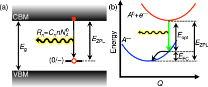
Figure 1: Illustration of radiative carrier capture in two different representations: (a) band diagram and (b) configuration coordinate diagram, for the case of a single acceptor defect $A$.

The radiative transition can also be represented via a configuration coordinate diagram [Fig. 1(b)]. The two charge states of the defect give rise to curves that are displaced along the horizontal axis because generally they have different atomic configurations (here projected on a one-dimensional coordinate $Q$). In the so-called Franck-Condon approximation, the transition occurs for fixed nuclear coordinates [see the green arrow in Fig. 1(b)] with energy $E_{\text{opt}}$. After the transition the defect is in a vibrationally excited state. This state will decay to the equilibrium state on the picosecond time scale via phonon-phonon interactions, losing the relaxation energy $E_{\text{FC}}=E_{\text{ZPL}}-E_{\text{opt}}$, called the Franck-Condon energy.

The strength of the electron-phonon coupling associated with an optical transition can be expressed in terms of the Huang-Rhys factor $S$ Huang and Rhys (1950), which quantifies the number of phonons emitted during the transition. In this work, we will consider defects with strong electron-phonon coupling ($S\gg 1$). For such defects, $E_{\text{opt}}$ corresponds to the peak of the PL spectrum Alkauskas et al. (2012). The general formalism to treat optical transitions in semiconductors is presented in textbooks (e.g., Ch. 5 of Ref. Ridley, 2013 or Ch. 10 of Ref. Stoneham, 2001). Here we will present a derivation of the capture coefficients specifically adapted to our implementation within first-principles electronic structure theory, and focusing on the case of strong electron-phonon coupling.

We will closely follow the reasoning previously applied in deriving nonradiative capture coefficients Alkauskas et al. (2014) [summarized in the supplemental material (SM) SM section S1], where it was shown that, for defects in the dilute limit, the capture coefficient can be expressed as

$$C_{n}=Vr,$$ (1)

where $r$ is the capture rate of one electron by one impurity in the volume $V$; the task is to calculate $r$.

II.2 Derivation of the capture coefficient

The wavefunctions describing the defect system are functions of all electronic $\{x\}$ and ionic $\{Q\}$ degrees of freedom; using the Born-Oppenheimer approximation, they can be written in the form $\Psi(\{Q\},\{x\})\chi(\{Q\})$, where $\Psi(\{Q\},\{x\})$ is the electronic wavefunction (which depends parametrically on $\{Q\}$), and $\chi(\{Q\})$ is the ionic wavefunction. Let the electronic wavefunction of the initial (excited) state, which in the case of the acceptor in Fig. 1 is the neutral defect plus the electron in the conduction band, be $\Psi_{i}(\{Q\},\{x\})$; the associated ionic wavefunctions are $\chi_{im}(\{Q\})$, where $m$ denotes the vibrational state. We will consider only transitions at low temperature, and therefore initially the system is in the ground vibrational state ($m=0$). The corresponding quantities for the final (ground) electronic state (the negatively charged defect, Fig. 1) are $\Psi_{f}(\{Q\},\{x\})$ and $\chi_{fn}(\{Q\})$. The expressions can be easily generalized to finite temperatures Stoneham (2001).

Optical transitions occur because of coupling to the electric field, described by the momentum matrix element $\textbf{P}_{if}(\{Q\})=\langle\Psi_{i}(\{Q\})|\hat{\textbf{P}}|\Psi_{f}(\{Q\})\rangle$; the momentum operator is $\hat{\textbf{P}}=-i\hbar\sum_{j}\partial/\partial\textbf{x}_{j}$, where the sum runs over all electrons $j$. We will use the Condon approximation (CA) Lax (1952), in which the dependence on $\{Q\}$ is neglected and the momentum matrix element is taken at a fixed $\{Q\}$ (which we choose to be the equilibrium geometry of the initial state); the validity of the CA will be discussed below.

An additional approximation is that multi-electron wavefunctions $\Psi_{\{i,f\}}$ can be replaced with single-particle Kohn-Sham orbitals $\psi_{i}$ and $\psi_{f}$, with corresponding momentum matrix element, $\textbf{p}_{if}$. In the case of electron capture, $\psi_{i}$ is a perturbed conduction-band state, while $\psi_{f}$ is a defect state. At finite temperature, electrons occupy a thermal distribution of states with different momenta; in principle, one has to average over this distribution. For non-degenerate semiconductors at room temperature these states are very close to the CBM, and thus we will approximate the initial state to be the CBM.

Within the Born-Oppenheimer approximation and the CA, the luminescence intensity (number of photons per unit time, per unit energy, for a given photon energy $\hbar\omega$) is given by Stoneham (2001)

$$I(\hbar\omega)= \frac{e^{2}n_{\text{r}}\omega\eta_{\text{sp}}}{3m^{2}\varepsilon_{0}\pi c^{3}\hbar}\left|p_{if}\right|^{2}$$ (2)

$$\times\sum_{n}\left|\left\langle\chi_{i0}|\chi_{fn}\right\rangle\right|^{2}\delta\left(E_{\text{ZPL}}-\hbar\omega_{fn}-\hbar\omega\right)\,.$$

$n_{\text{r}}$ is the index of refraction, $\hbar\omega_{fn}$ is the energy of the final vibrational state (with respect to its ground state), and $\eta_{\text{sp}}$ is a factor which accounts for the spin selection rule ($\eta_{sp}$=1 for a transition from a spin-singlet to a doublet, $\eta_{sp}$=0.5 for a transition from a doublet to a singlet or from a triplet to a doublet). The total recombination rate is the integral of $I(\hbar\omega)$ over energy $\hbar\omega$:

$$r=\frac{e^{2}n_{r}\eta_{\text{sp}}}{3m^{2}\varepsilon_{0}\pi c^{3}\hbar^{2}}\left|p_{if}\right|^{2}\langle\hbar\omega\rangle\,,$$ (3)

where $\langle\hbar\omega\rangle=\sum_{n}\left|\langle\chi_{i0}|\chi_{fn}\rangle\right|^{2}(E_{ZPL}-\hbar\omega_{fn})$ is the average energy of emitted photons. In the case of strong electron-phonon coupling, $\langle\hbar\omega\rangle$ coincides with the energy of the vertical transition $E_{\text{opt}}$ [green arrow in Fig. 1(b)]. For defects studied in this work $S>8$, so we will make this approximation.

Combining Eq. (1) and Eq. (3) gives the capture coefficient if the quantities in Eq. (3) could be calculated in a large volume $V$ corresponding to the dilute limit of defects; in practice, calculations are performed in supercells with much smaller volumes $\widetilde{V}$. The limited supercell size is not an issue for describing capture at neutral defects. However, in the case of charged defects the initial electronic state is not properly described. This issue can be accounted for by scaling Eq. (3) by the so-called Sommerfeld factor $f$ Bonch-Bruevich (1959); Pässler (1976); Alkauskas et al. (2014). In this work, only neutral centers are considered, so $f=1$.

The final expression for the capture coefficient is:

$$\begin{split}C_{n}&=f\eta_{\text{sp}}\widetilde{V}\frac{e^{2}n_{\text{r}}}{3m^{2}\varepsilon_{0}\pi c^{3}\hbar^{2}}\left|p_{if}\right|^{2}E_{\text{opt}}\\ &=\left(5.77\times 10^{-17}\right)\left(\widetilde{V}fn_{r}\eta_{\text{sp}}E_{\text{opt}}\frac{|p_{if}|^{2}}{2m}\right)\text{cm}^{3}\text{s}^{-1}\end{split}$$ (4)

where in the second line we have evaluated the material-independent parameters (assuming $E_{\text{opt}}$ and $|p_{if}|^{2}/2m$ are expressed in eV, and $\widetilde{V}$ in ų) resulting in a simple formula that can be used to evaluate radiative capture coefficients based on quantities generated by density functional theory calculations. Equation (4) agrees with the expression used in Ref. Zhang et al., 2017, except for the fact that the spin selection rules are neglected in that work (e.g., for carbon on the N site in GaN, this results in an extra factor of two in Ref. Zhang et al., 2017).

III Results

III.1 Computational details

We have calculated $E_{\rm opt}$ and $\textbf{p}_{if}$ necessary for Eq. (4) using density functional theory with the hybrid functional of Heyd, Scuseria, and Ernzerhof (HSE) Heyd et al. (2006). The mixing parameter was chosen to reproduce the experimental band gaps: 0.30 for GaAs (giving a band gap of 1.52 eV) and 0.31 for GaN (giving a band gap of 3.50 eV). Ga 3$d$ electrons were treated as core states. Defect calculations were performed on 216-atom zincblende supercells for GaAs, and 96-atom wurtzite supercells for GaN. When optimizing the defect geometry the Brillouin zone was sampled with a single special $k$-point (1/4,1/4,1/4) Monkhorst and Pack (1976). Since for non-degenerately doped GaN and GaAs the electrons participating in capture originate from the CBM, momentum matrix elements were evaluated at the $\Gamma$ point. Use of the $\Gamma$ point also correctly captures the symmetries of the system. We used the Vienna ab-initio Simulation Package (VASP)Kresse and Furthmüller (1996) with the projector augmented wave (PAW) method Blöchl (1994); for the transition matrix elements, the methodology of Ref. Gajdoš et al., 2006 was used, (i.e., momentum matrix elements are correctly calculated for the case of nonlocal potentials). Thermodynamic charge-state transition levels of the defects ($E_{\text{ZPL}}$ in Fig. 1) and $E_{\text{opt}}$ were calculated using the standard methodology described in Ref. Freysoldt et al., 2014, where we use the scheme of Refs. Freysoldt et al., 2009 and Freysoldt et al., 2011 to correct for interactions between charged defects and their periodic images. We use experimental indices of refraction (3.4 for GaAs Skauli et al. (2003) and 2.4 for GaN Kawashima et al. (1997), consistently chosen for energies $E_{\text{opt}}$).

III.2 Capture coefficients of test-case defects

We test the methodology on two defects for which extensive experimental information is available: the complex between a Ga vacancy and a Te donor on a nearest-neighbor As site in GaAs, GaAs:$V_{\text{Ga}}$-$\text{Te}_{\text{As}}$, Glinchuk et al. (1977) and a carbon substitutional impurity on a nitrogen site in GaN, GaN:C${}_{\text{N}}$ Ogino and Aoki (1980); Reshchikov (2014) (see Secs. S2 and S3 of SM SM for details of the experimental identification). In both cases, we examine the rate of electron capture for the neutral charge state.

We calculate the energy of the $(0/-)$ thermodynamic charge-state transition levelFreysoldt et al. (2014), at which electron capture occurs, to be $0.37$ eV above the VBM for GaAs:$V_{\text{Ga}}$-$\text{Te}_{\text{As}}$ and $1.02$ eV for GaN:C${}_{\text{N}}$. The calculated and experimental optical transition energies are given in Table 1. A detailed description of the electronic structure of GaN:C${}_{\text{N}}$ and GaAs:$V_{\text{Ga}}$-$\text{Te}_{\text{As}}$ is provided in Sec. S4 of the SM SM .

Table 1: Calculated (Calc.) and experimentally measured (Exp.) optical transition energies $E_{\rm ZPL}$ and $E_{\rm opt}$ and electron capture coefficients $C_{n}$ for the two defects in our case studies.

	$E_{\rm ZPL}$ (eV)		$E_{\rm opt}$ (eV)		$C_{n}$ ($10^{-13}$ cm3s-1)
	Calc.	Exp.	Calc.	Exp.	Calc.	Exp.
GaAs:$V_{\text{Ga}}$-$\text{Te}_{\text{As}}$	1.23	1.38	1.02	1.18	3.5	6.5
GaN:C${}_{\text{N}}$	2.48	2.57	2.01	2.2	0.7	$0.6-1.2$

Our calculated capture coefficients using Eq. (4) are given in Table  1 along with experimental values. The calculated value for GaN:C${}_{\text{N}}$ of $C_{n}=0.7\times 10^{-13}$ cm³s^-1, is in good agreement with measurements by Reshchikov et al. Reshchikov (2014); Reshchikov et al. (2016) that yield values $(0.6-1.2)\times 10^{-13}$ cm³s^-1 for radiative capture coefficients pertaining to yellow luminescence in GaN (different values are for different samples). Therefore, our calculations indicate that GaN:C${}_{\text{N}}$ is the likely source of the yellow luminescence in the samples studied by Reshchikov Reshchikov (2014).

Our value for $C_{n}$ is about a factor of four smaller than the one calculated in Ref. Zhang et al., 2017, which is mainly due to the fact that $\eta_{\text{sp}}$ is not included in that work. Additionally, we find a slightly smaller value of $|p_{if}|^{2}$ (0.03 versus 0.05 in Ref. Zhang et al., 2017), and a different value for the refractive index may have been used. We note that inclusion of $\eta_{sp}$ (i.e., application of the spin selection rules) is important and necessary to obtain agreement with experiment.

For GaAs:$V_{\text{Ga}}$-$\text{Te}_{\text{As}}$, we find that $C_{n}=3.5\times 10^{-13}$ cm³s^-1, five times larger than for GaN:C${}_{\text{N}}$. Our calculated value is in satisfactory agreement with the value determined experimentally by Glinchuk et al.Glinchuk et al. (1977) ($C_{n}=6.5\times 10^{-13}$ cm³s^-1).

In order to test convergence with supercell size, we determined $C_{n}$ for the case of GaN:C${}_{\text{N}}$ using a matrix element $\textbf{p}_{if}$ calculated in supercells with various sizes. A 72-atom supercell results in $C_{n}=0.29\times 10^{13}$ cm³s^-1, while a 300-atom supercell, gives $C_{n}=0.90\times 10^{13}$ cm³s^-1. This indicates that the results for the supercells used in this study are close to converged.

In Sec. S5 of the SM SM , we compare these HSE results to those obtained using a generalized gradient functional, demonstrating the necessity of hybrid functionals for such quantitative accuracy.

IV Discussion

IV.1 Accuracy of the Condon approximation

As mentioned above, the derivation of Eq. (4) relies on the validity of the CA, which states that the transition matrix element does not change with configuration coordinate. We now test this assumption for the two case studies by calculating $|p_{if}|$ for different $Q$ values (Fig. 2). The generalized configuration coordinate chosen is a linear interpolation of all atomic positions between the ground-state structures of the neutral and negatively charged defects. This choice of $Q$ has been demonstrated to yield accurate PL lineshapes Alkauskas et al. (2012), indicating that it is a good approximation for the sum over all vibrational degrees of freedom.

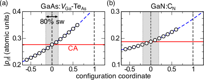
Figure 2: Dependence of the momentum matrix elements $p_{if}$ on configuration coordinate $Q$ for test-case defects (a) GaAs:$V_{\text{Ga}}$-$\text{Te}_{\text{As}}$ and (b) GaN:C${}_{\text{N}}$. The blue dashed line represents a quadratic fit to the data. The gray vertical bar indicates the spread of $Q$ values that gives rise to 80 % of the spectral weight (sw). The horizontal line indicates the Condon approximation (CA), in which the matrix element is taken to be constant.

In Fig. 2 the CA is indicated by the red horizontal line, reflecting the $|p_{if}|$ values at $Q$=0 (the equilibrium geometry of the initial state). In order to estimate the error we make by using the CA, we must have some measure of the importance that $Q$ values other than $Q$=0 carry in a full determination of the transition rate. Such a measure is obtained by calculating the ground-state vibrational wavefunction in the initial state [$(A^{0}+e^{-})$ in Fig. 1(b)], the square of which is roughly proportional to the spectral weight of the optical transition at a given $Q$. We then consider the variation of the matrix elements over the region containing $80\%$ of the spectral weight of the transition (gray shaded region in Fig. 2). We see that most of the spectral weight of the transition is concentrated near the vertical transition at $Q$=0; this is generally true for defects with large Huang-Rhys factors, such as the ones considered here. The matrix element $|p_{if}|$ varies by $\sim 14\%$ over the gray range for both defects (Fig. 2), translating into an error in $C_{n}$ of less than 14%, which is acceptable and well within the experimental uncertainty. It remains to be seen if the accuracy of the CA holds for other deep defects.

IV.2 Implications for Shockley-Read-Hall recombination

The results in Table 1 provide important information about the role of radiative capture in defect-assisted SRH recombination processes. In Ref. Dreyer et al., 2016, it was shown that for defect densities of $10^{16}$ cm^-3, capture coefficients larger than $10^{-10}$ cm³s^-1 are necessary to result in SRH recombination rates that would compete with electron-hole radiative recombination and significantly impact the performance of light-emitting diodes. If we use this magnitude as a threshold, we see that for the defects in Table 1 the radiative electron capture rates are much too slow (by three orders of magnitude) to give rise to detrimental SRH recombination. We suggest that this conclusion may be more general. Based on the character of the wavefunctions, we expect the optical transition matrix elements for our case-study defects to be fairly strong, and hence it seems unlikely that $|p_{if}|^{2}/2m$ values for other defects (including in other hosts) would be orders of magnitude larger. Furthermore, Eq. (4) shows that $C_{n}$ depends only linearly on $E_{\text{opt}}$. Both observations indicate that radiative capture coefficients are unlikely to be high enough to give rise to strong defect-assisted SRH recombination.

IV.3 Comparison to model calculations

We now discuss how our methodology and implementation differ from previous attempts at theoretical descriptions of optical transitions for defects in semiconductors. Previous methods relied on models for the defect wavefunction in order to determine $\textbf{p}_{if}$ Ridley (2013). An often-used model for deep defects is the “quantum defect” (QD) model Bebb (1969); Bebb and Chapman (1971); Lucovsky (1965), where the defect potential near the core is treated as a square well, while the long-range part has the form of a Coulomb potential. It can be shown (see Sec. S6 of the SMSM ) that, for capture of an electron at a neutral acceptor, the QD model results in a form of the capture coefficient similar to Eq. (4), but with the key difference that $|p_{if}|^{2}$ is replaced by the momentum matrix element between the bulk conduction and valence bands $|p_{cv}|^{2}$. The matrix element is then scaled by an “effective volume” describing the spatial extent of the defect wavefunction. In addition, the QD model uses the zero-phonon line energy ($E_{\text{ZPL}}$) of the defect instead of $E_{\text{opt}}$; i.e., the Frank-Condon relaxation energy, resulting from the coupling with the lattice, is neglected.

We now compare capture coefficients calculated with the QD model with our full first-principles results. The equations and parameters are included in Sec. S6 of the SMSM . We find that for GaN:C${}_{\text{N}}$, $C_{n}^{\text{QD}}=0.4\times 10^{-13}$ cm³s^-1, which is smaller than our first-principles value (Table 1), and slightly below the experimental range. For GaAs:$V_{\text{Ga}}$-$\text{Te}_{\text{As}}$, $C_{n}^{\text{QD}}=10.2\times 10^{-13}$, slightly larger than the first-principles value and overestimating the experimental value. While for these case studies the model agrees reasonably well with first-principles results, it is important to emphasize the limited predictive power of models such as the QD model. First, they require energy levels taken either from experiment or from first-principles calculations. Second, since $|p_{if}|$ is replaced with $|p_{cv}|$, specific information about the defect electronic structure is lost, and assumptions about the character of the defect wavefunction are required. In our case studies, the assumption that, as acceptors, the wavefunctions have valence-band character turns out to be reasonable, but this will not universally be the case.

V Conclusions

We have demonstrated a methodology for determining capture coefficients from first principles. For the two case studies considered, GaAs:$V_{\text{Ga}}-\text{Te}_{\text{As}}$ and GaN:C${}_{\text{N}}$, the calculations give quantitative agreement with experimental measurements. We also confirmed the validity of the Condon approximation, a result that can be generalized to all defects with large values of the Huang-Rhys factor. The procedure outlined in this work will provide a tool for the identification and characterization of defects detected by optical spectroscopy, and aid in identifying the origins and mechanisms of Shockley-Read-Hall recombination.