Mott metal-insulator transition from steady-state density functional theory

Abstract

We present a computationally efficient method to obtain the spectral function of bulk systems in the framework of steady-state density functional theory (i-DFT) using an idealized Scanning Tunneling Microscope (STM) setup. We calculate the current through the STM tip and then extract the spectral function from the finite-bias differential conductance. The fictitious non-interacting system of i-DFT features an exchange-correlation (xc) contribution to the bias which guarantees the same current as in the true interacting system. Exact properties of the xc bias are established using Fermi-liquid theory and subsequently implemented to construct approximations for the Hubbard model. We show for two different lattice structures that the Mott metal-insulator transition is captured by i-DFT.

Introduction.– Standard wisdom has it that density functional theory (DFT) DreizlerGross:90 is not capable of describing strongly correlated materials. The origin of this misconception is twofold. By construction, the exact exchange-correlation (xc) potential of the Kohn-Sham (KS) system yields the exact electronic density and directly related quantities. However, approximations to the xc potential often miss the step features due to the derivative discontinuity of the generating xc energy functional PerdewParrLevyBalduz:82 . These features are a crucial ingredient to capture strong correlation effects in diverse physical situations such as, e.g., molecular dissociation RuzsinszkyPerdewCsonkaVydrovScuseria:06 ; FuksMaitra:14 , fermion gases in optical lattices Xianlong_etal:06 or transport StefanucciKurth:11 ; BergfieldLiuBurkeStafford:12 ; TroesterSchmitteckertEvers:12 ; KurthStefanucci:13 ; KurthStefanucci:17 ; DittmannSplettstoesserHelbig:18 ; DittmannHelbigKennes:19 . Approximations which include the steps are under active development MirtschinkSeidlGoriGiorgi:13 ; KraislerKronik:13 ; BroscoYingLorenzana:13 ; YingBroscoLorenzana:14 ; Sobrino:PRB:2020 . Furthermore, the interpretation of the KS excitation energies as true excitation energies is not rigorously justified, even if the exact xc potential is used. While in the limit of weak correlations this may be a reasonable approximation, it completely fails in the opposite limit – it is easy to show that the exact KS band structure of the Hubbard model in the Mott insulating phase has no gap and the derivative discontinuity plays a crucial role in describing the Mott transition LimaSilvaOliveiraCapelle:03 ; KarlssonPriviteiraVerdozzi:11 ; KVOC.2011 ; KKPV.2013 .

In general, extracting excitation energies in a DFT framework is not straightforward. While charge neutral excitations are accessible via time-dependent (TD) DFT RungeGross:84 ; Ullrich:12 , excitations which do change the number of electrons such as those probed in (inverse) photoemission are encoded in the spectral function, an arduous quantity to calculate also for TDDFT Uimonen_2014 . Usually spectral functions are calculated within a Green’s function framework MartinReiningCeperley:16 ; svl-book , e.g. GW Aryasetiawan_1998 ; GolzeDvorakRinke_2019 , Dynamical Mean-Field Theory (DMFT) Metzner:PRL:1989 ; Georges:PRB:1992 ; Georges:RMP:1996 and GW+DMFT Biermann:PRL:2003 ; Biermann_2014 , but these methods come at considerable computational cost. Instead, DMFT combined with DFT offers a pragmatic approach to compute the spectra of strongly correlated materials Lichtenstein_1998 ; Vollhardt_2005 ; Kotliar:RMP:2006 , although the double counting problem remains unsolved.

Recently we proposed a method to compute the spectral function JacobKurth:18 of a nanoscale tunneling junction using an extension of DFT, called steady-state DFT or i-DFT StefanucciKurth:15 . In i-DFT the fundamental variables are the non-equilibrium steady-state density of and current through the junction. Hence the KS system requires a nonequilibrium extension of the standard xc potential as well as the introduction of an xc contribution to the applied bias in the electrodes sa-1.2004 ; sa-2.2004 ; SaiZwolakVignaleDiVentra:05 ; KoentoppBurkeEvers:06 . In an idealized Scanning Tunneling Microscope (STM) setup where one of the electrodes (i.e. the “STM tip”) couples only weakly to the nanoscale junction, the spectral function at frequency $\omega$ can be obtained from the differential conductance at bias $V=\omega$ JacobKurth:18 ; KurthJacobSobrinoStefanucci:19 .

In this Letter we generalize the i-DFT+STM approach to calculate the spectral function of arbitrary bulk systems. We further show that the Mott metal-insulator (MI) transition in the Hubbard model, one of the main paradigms in the field of strongly correlated electrons, can be described by i-DFT provided that both the xc potential and the xc bias feature steps as function of the steady density and current. General properties of the xc bias are derived using Fermi liquid (FL) theory in combination with DMFT Metzner:PRL:1989 ; Georges:PRB:1992 ; Georges:RMP:1996 . Taking advantage of ideas developed previously in the context of the Anderson impurity model StefanucciKurth:15 ; KurthStefanucci:16 we construct an approximation satisfying all FL+DMFT properties and illustrate the MI transition in two different crystal structures, the Bethe and the cubic lattices.

Bulk spectral function from i-DFT.– We consider a bulk system described by a Hamiltonian written in terms of creation and annihilation operators for electrons with spin projection $\sigma$ in basis functions $\{\varphi_{i}\}$. The basis functions are taken orthonormal but otherwise completely general – they can be, e.g., extended Bloch states or localized Wannier functions. No assumptions on the explicit form of the Hamiltonian is made at this stage. The system is probed by an ideal nonmagnetic tip, a fictitious “Gedanken” device with the following properties: (i) the electrons in the tip are noninteracting with energy dispersion $\epsilon_{k}$ and wavefunctions $\psi_{k}$. This property ensures the applicability of the Meir-Wingreen formula MeirWingreen:92 for the steady current from the tip to the bulk JacobKurth:18 ; (ii) the coupling of the tip to the bulk is weak but otherwise its form can be chosen freely. For convenience, here we take it to be coupled exclusively to the $n$-th basis function $\varphi_{n}$ of the bulk. Letting $T_{k}$ be the one-electron integral between the states $\psi_{k}$ and $\varphi_{n}$, the ideal tip is chosen to have a transition rate $\gamma=2\pi\sum_{k}|T_{k}|^{2}\delta(\omega-\epsilon_{k})$ independent of $\omega$ (wide band limit). Without any loss of generality we set the chemical potential of the whole system (tip plus bulk) to zero. A bias $V$ is applied only in the tip and as a consequence a steady current $I(V)$ flows toward the bulk through state $\varphi_{n}$. In the limit of vansihing coupling, the bulk remains in equilibrium and its spectral function projected onto the state $\varphi_{n}$ can then be written as JacobKurth:18

$$A(\omega)=\lim_{\gamma\to 0}\frac{\pi}{\gamma}\left.\frac{dI(V)}{dV}\right|_{V=\omega}.$$ (1)

Here we use i-DFT to compute $I(V)$. In i-DFT the bulk density for a given potential $v$ and the steady current for a given bias $V$ are reproduced in the same but noninteracting bulk system coupled to the same tip. This fictitious KS system is subject to the effective potential $v_{s}=v+v_{\rm Hxc}$, where $v_{\rm Hxc}$ is Hartree plus exchange-correlation (Hxc) potential, and to the effective bias $V_{s}=V+V_{\rm xc}$ with $V_{\rm xc}$ the xc bias. Both $v_{\rm Hxc}$ and $V_{\rm xc}$ are functionals of the bulk density and the steady current. However, in the $\gamma\to 0$ limit, see Eq. (1), $v_{\rm Hxc}$ becomes independent of $I$ and approaches the ground-state Hxc potential of DFT JacobKurth:18 . In what follows we assume that $v_{\rm Hxc}$ is known from a previous DFT calculation. Denoting by $A_{s}(\omega)$ the ground-state KS spectral function we then have

$$\lim_{\gamma\to 0}\frac{I}{\gamma}=\int\frac{d\omega}{\pi}[f(\omega-V-V_{\rm xc})-f(\omega)]A_{s}(\omega).$$ (2)

For any given bias $V$ this equation must be solved self-consistently since $V_{\rm xc}$ depends on $I$. The relation between $A$ and $A_{s}$ follows directly from the derivative of Eq. (2) with respect to $V$

$$A(\omega)=\lim_{\gamma\to 0}\frac{A_{s}(\omega+V_{\rm xc})}{1-\frac{\gamma}{\pi}\frac{dV_{\rm xc}}{dI}A_{s}(\omega+V_{\rm xc})}=A_{s}(\Omega)\frac{d\Omega}{d\omega}$$ (3)

where $\Omega(\omega)=\omega+V_{\rm xc}[I(\omega)]$. Equation (3) is one of the main results of this Letter and shows that i-DFT can be used to calculate bulk spectral functions.

Properties of the xc bias from Fermi-liquid theory.– For i-DFT to become a practical and computationally efficient scheme we need to develop accurate approximations to $V_{\rm xc}$. Any approximation should satisfy $V_{\rm xc}[0]=0$, for otherwise there would be a finite current at zero bias. Below we derive a few more properties for uniform systems from FL theory and DMFT. We concentrate on the local description (hence $\varphi_{n}$ is a site basis function) and use DMFT which becomes exact in the limit of infinite dimensions (or, more rigorously, coordination number) Metzner:PRL:1989 ; Georges:PRB:1992 ; Georges:RMP:1996 – and otherwise yields a very good approximation for dimensions $\geq 3$ Florens:PRB:2004 .

Due to the Friedel sum rule mera-2 ; Schmitteckert:PRL:2008 ; TroesterSchmitteckertEvers:12 , the spectral function evaluated at the Fermi energy depends only on the bulk density. As the latter is the same in the many-body and the KS system we have $A(0)=A_{s}(0)$. Since $I(0)=0$ then $\Omega(0)=V_{\rm xc}[0]=0$ and therefore Eq. (3) implies

$$\left.\frac{dV_{\rm xc}}{dI}\right|_{I=0}=0.$$ (4)

Other properties can be obtained for particle-hole (ph) symmetric systems, e.g., the half-filled Hubbard model on bipartite lattices. In DMFT the local Green’s function can be written as $G^{-1}(\omega)=\omega-v-\tilde{\Sigma}(\omega)-\Delta_{0}(\omega)$ where $v$ is the uniform potential, $\Delta_{0}(\omega)=\Lambda_{0}(\omega)-i\Gamma_{0}(\omega)/2$ the noninteracting embedding self-energy (or hybridization function) and $\tilde{\Sigma}(\omega)$ the many-body self-energy. We emphasize that $\tilde{\Sigma}(\omega)$ is not the local DMFT self-energy $\Sigma(\omega)$ as it contains also correlation corrections to the embedding:

$$\tilde{\Sigma}=\Sigma+\Delta-\Delta_{0}.$$ (5)

At half-filling the spectral function $A(\omega)=i[G(\omega)-G^{\ast}(\omega)]$ is an even function of frequency. Additionally, the ph symmetry yields a condition for the Hxc potential, i.e., $v_{\rm Hxc}=-v$. Hence the KS Green’s function is simply $G_{s}(\omega)=\left[\omega-\Delta_{0}(\omega)\right]^{-1}$ and therefore the KS spectral function $A_{s}(\omega)=i[G_{s}(\omega)-G_{s}^{\ast}(\omega)]$ is even too.

Differentiating Eq. (3), evaluating the result in $\omega=0$ and using $A^{\prime}(0)=A^{\prime}_{s}(0)=0$ (henceforth primes are used to denote derivatives with respect to $\omega$) we find $A_{s}(0)\Omega^{\prime\prime}(0)=0$. Using $A_{s}(0)=A(0)=\lim_{\gamma\to 0}\frac{\pi}{\gamma}I^{\prime}(0)\neq 0$, see Eq. (1), then yields

$$\Omega^{\prime\prime}(0)=\left.\frac{d^{2}V_{\rm xc}}{dI^{2}}\right|_{I=0}I^{\prime}(0)^{2}+\left.\frac{dV_{\rm xc}}{dI}\right|_{I=0}I^{\prime\prime}(0)=0.$$ (6)

Taking further into account Eq. (4), this implies that also the second derivative of $V_{\rm xc}$ w.r.t. the current should vanish:

$$\left.\frac{d^{2}V_{\rm xc}}{dI^{2}}\right|_{I=0}=0.$$ (7)

The third derivative of $V_{\rm xc}$ w.r.t. the current is nonvanishing and can be related to the pseudo quasi-particle weight

$$\tilde{Z}^{-1}\equiv 1-{\rm Re}[\tilde{\Sigma}^{\prime}(0)].$$ (8)

In the Supplemental Material  we prove that

$$\left.\frac{d^{3}V_{\rm xc}}{dI^{3}}\right|_{I=0}=-\frac{\pi^{3}\Gamma_{0}(0)}{8\gamma^{3}}\left[(\tilde{Z}^{-1}-\Lambda^{\prime}_{0}(0))^{2}-(1-\Lambda^{\prime}_{0}(0))^{2}\right].$$ (9)

We shall use the properties in Eqs. (4), (7) and (9) to construct approximations to the xc bias.

We observe that the pseudo quasi-particle weight can be expressed in terms of the actual quasi-particle weight $Z\equiv[1-{\rm Re}[\Sigma^{\prime}(0)]^{-1}$ through Eq. (5): $\tilde{Z}^{-1}=Z^{-1}-{\rm Re}[\Delta^{\prime}(0)]+{\rm Re}[\Delta_{0}^{\prime}(0)]$. In DMFT the interacting embedding self-energy (or hybridization function) $\Delta(\omega)$ is related to the local Green’s function $G(\omega)=N^{-1}\sum_{k}(\omega-\epsilon_{k}-\Sigma(\omega))^{-1}$ via the Dyson equation $\Delta(\omega)=\omega-v-\Sigma-[G(\omega)]^{-1}$. Differentiation and evaluation at $\omega=0$ then yields $\Delta^{\prime}(0)=Z^{-1}+G^{\prime}(0)/[G(0)]^{2}$. While $G(0)=G_{s}(0)$ by Friedel sum rule, it is straightforward to show Note1 that $G^{\prime}(0)=Z^{-1}G_{s}^{\prime}(0)$. Thus

$$\tilde{Z}^{-1}=1+\frac{Z-1}{Z}\cdot\frac{G_{s}^{\prime}(0)}{[G_{s}(0)]^{2}}$$ (10)

which can be easily evaluated since $G_{s}(\omega)$ depends only on the lattice properties through $\Delta_{0}(\omega)$.

The xc bias for the metal-insulator transition.– We consider the half-filled Hubbard model on the Bethe lattice (BL) with infinite coordination number as well as on a cubic lattice (CL), and describe the strategy common to the construction of the xc bias for both lattices.

In the insulating Mott phase the Hubbard bands become Coulomb blockade (CB) peaks as the hopping integral between neighboring sites decreases. In the limit of vanishing hopping the CB peaks are separated in energy by the Hubbard interaction $U$. For finite hopping the CB peaks are separated by the discontinuity $U_{\rm xc}$ of the Hxc potential (with $\lim_{U\to\infty}U_{\rm xc}(U)/U=1$). The xc bias should feature a step of height $U_{\rm xc}$ JacobKurth:18 ; KurthJacob:18 ,

$$\bar{V}_{\rm xc}[I]=-\frac{U_{\rm xc}}{2}{\rm sign}(\tilde{I})-(U-U_{\rm xc})g(\tilde{I})\;.$$ (11)

Here we have defined the reduced current as $\tilde{I}=I/(2\gamma)$ and its physically realizable domain is $\tilde{I}\in(-\frac{1}{2},\frac{1}{2})$. The function $g(\tilde{I})$ depends on the lattice and fulfills the general properties: (i) $g(-\tilde{I})=-g(\tilde{I})$, and (ii) $g(\pm\frac{1}{2})=\pm\frac{1}{2}$ such that $\bar{V}_{\rm xc}[\pm\gamma]=\mp\frac{U}{2}$. In the SI we describe the strategy to obtain $U_{\rm xc}(U)$ and $g(\tilde{I})$ for both the Bethe and the cubic lattice.

The approximation in Eq. (11) violates the property in Eq. (4) which is crucial for describing the Kondo peak in the metallic phase KurthStefanucci:16 . We then make the ansatz

$$V_{\rm xc}[I]=a(I)\bar{V}_{\rm xc}[I].$$ (12)

For $I$ close to zero we can approximate $\bar{V}_{\rm xc}[I]\simeq-\frac{U_{\rm xc}}{2}{\rm sign}(\tilde{I})$. If $\tilde{I}$ is nonnegative we can rewrite this expression as the limiting function of the sequence $\bar{V}^{(n)}_{\rm xc}[I]=-\frac{U_{\rm xc}}{2}\tilde{I}^{1/n}$. Letting $\alpha\tilde{I}^{p}$ be the leading order term of the function $a(I)$ as $\tilde{I}\to 0^{+}$ we have $V^{(n)}_{\rm xc}[I]\simeq-\frac{\alpha U_{\rm xc}}{2}\tilde{I}^{p+1/n}$. We then see that the properties in Eqs. (4), (7) and (9) are fulfilled provided that $p=3+1/n$. Taking the limit $n\to\infty$ and using that $a(I)=a(-I)$ we infer that for $I\simeq 0$ the function $a(I)\simeq\alpha|\tilde{I}|^{3}$. In the following we parametrize this function as

$$a(I)=\frac{2}{\pi}{\rm atan}\left(|\lambda_{\rm K}\tilde{I}|^{3}\right)$$ (13)

since for $|\tilde{I}|=1/2$ we must have $a(I)\simeq 1$ for $V_{\rm xc}[\pm\gamma]\simeq\mp\frac{U}{2}$. Taking into account that

$$\left.\frac{d^{3}V_{\rm xc}}{dI^{3}}\right|_{I=0}=-\frac{3U_{\rm xc}}{4\pi\gamma^{3}}\lambda_{\rm K}^{3},$$ (14)

the parameter $\lambda_{\rm K}\gg 1$ can be determined from Eq. (9).

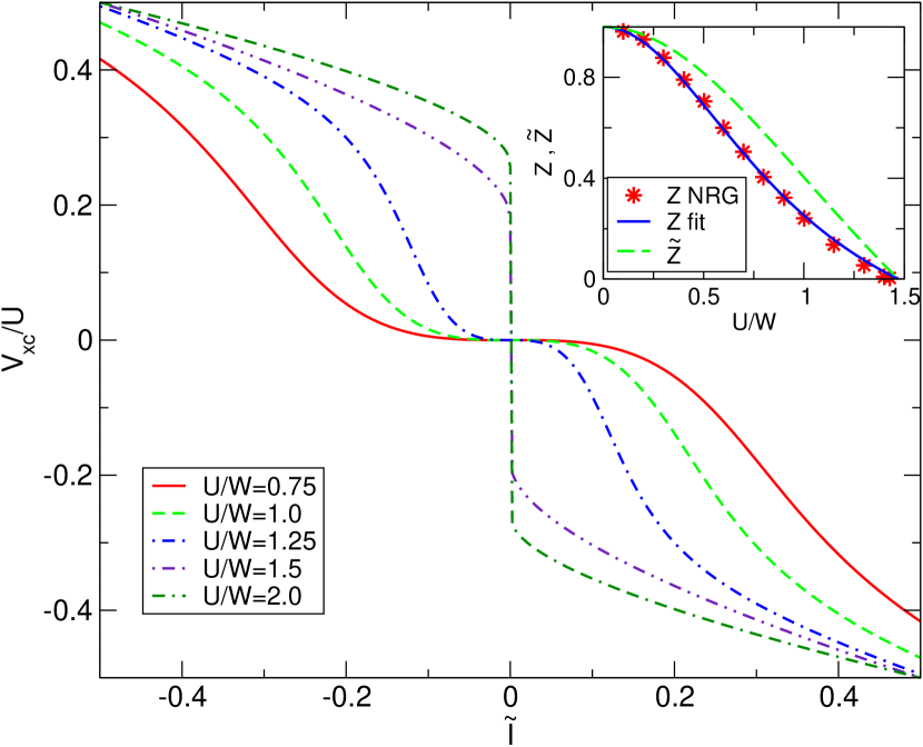
Figure 1: Model xc bias of Eq. (12) for the Bethe lattice for different values of $U$. Inset: Quasiparticle weights $Z$ from NRG of Ref. Bulla:99 , our fit to the NRG data as well as $\tilde{Z}$ according to Eq. (10). $W$ is the width of the band for $U=0$.

We apply the i-DFT approach to the calculation of the spectral function of the Hubbard model on a BL and CL. To obtain $\bar{V}_{\rm xc}[I]$ in Eq. (11) we performed DMFT calculations for both lattices using the non-crossing approximation (NCA) PruschkeCoxJarrell:93 in the insulating phase. Reverse engineering the DMFT+NCA spectral function Note1 we found that an accurate parametrization is provided by

$$g(\tilde{I})=\left((1-b)\sqrt{|\tilde{I}/2|}+b\tilde{I}\right){\rm sign}(\tilde{I}),$$ (15)

with $b=1/4$ in the BL and $b=0$ in the CL, whereas $U_{\rm xc}(U)$ is a smooth increasing function of $U$, see Ref. Note1 for the explicit form. To determine $\lambda_{\rm K}$ and hence the function $a(I)$ we first consider a BL. In this case $\Delta_{0}(\omega)=\frac{\omega}{2}-i\sqrt{\left(\frac{W}{4}\right)^{2}-\left(\frac{\omega}{2}\right)^{2}}$, where $W$ is the bandwidth; hence $\Lambda^{\prime}(0)=1/2$ and $\Gamma_{0}(0)=W/2$. Inserting these values in Eq. (9) and using Eq. (14) we obtain

$$\lambda_{\rm K}^{3}=\frac{\pi^{4}W}{12U_{\rm xc}}\frac{1-\tilde{Z}}{\tilde{Z}^{2}}.$$ (16)

Close to zero frequency the BL Green’s function $G(\omega)=(4/W)^{2}\Delta(\omega)\simeq Z/(\omega-Z\Delta(\omega))$, which implies $\Delta(\omega)=\Delta_{0}(\omega/Z)$; hence from Eq. (10)

$$\tilde{Z}=\frac{2Z}{1+Z}.$$ (17)

The quasi-particle weight has been accurately calculated in Ref. Bulla:99, using NRG, and it is well approximated by a shifted Lorentzian Note1 . In the inset of Fig. 1 we show the NRG $Z$, our fit and the pseudo quasi-particle weight $\tilde{Z}$. Proceeding along the same lines we constructed the xc bias for a CL, see Ref. Note1 for details. We anticipate that $\tilde{Z}(Z)$ is almost identical in the two lattices.

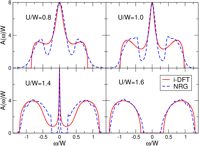
Figure 2: Spectral functions of the Hubbard model on the Bethe lattice for different interaction strengths obtained by i-DFT and compared with the NRG results of Ref. ZitkoPruschke:09 . $W$ is the width of the band for $U=0$.

Results.– In Fig. 1 we show the BL xc bias for different values of $U$ in units of the non-interacting bandwidth $W$. In the metallic phase, $U/W<1.3$, $V_{\rm xc}$ exhibits a plateau around $\tilde{I}=0$ which turns into a sharp step in the insulating phase. The development of a step is essential for the gap opening, see below.

In Fig. 2 we compare the i-DFT spectral functions with NRG results from Ref. ZitkoPruschke:09, for different interaction strengths. i-DFT captures the essential features of the spectra such as the Kondo peak at $\omega=0$ in the metallic phase as well as its disappearance with increasing interaction strength. The curvature of the Kondo peak at $\omega=0$ is, by construction, correctly described by our xc bias but also the Hubbard side bands are captured reasonably well, especially for large $U$’s. The approximation to $V_{\rm xc}$ performs poorly in the frequency range of the minima of $A(\omega)$ and some of the finer features of the NRG spectra are also missing. Interestingly, however, the i-DFT spectra always have finite support. This can be understood from Eq. (3) by noting that (i) $A_{s}(\omega)$ has finite support and (ii) the xc bias is restricted to the intervall $V_{\rm xc}\in[-\frac{U}{2},\frac{U}{2}]$.

The performance of the approximate xc bias for a CL is illustrated in Fig. 3 where we again compare i-DFT and NRG ZitkoBoncaPruschke:09 spectral functions for different interaction strengths. The general trend is similar to the previous case, in particular the MI transition is correctly captured. One feature which draws attention is the presence of “kinks” in the i-DFT spectra which are directly attributable to the van Hove singularities in the KS density of states.

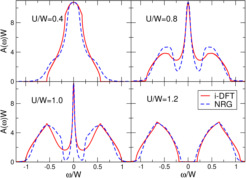
Figure 3: Spectral functions of the Hubbard model on the simple cubic lattice for different interaction strengths obtained by i-DFT and compared with the NRG results of Ref. ZitkoBoncaPruschke:09 .

Conclusions.– In summary, we have shown how one can extract bulk spectral functions from i-DFT. A particular emphasis has been on the proper description of the Mott metal-insulator transition in strongly correlated systems which so far has been elusive within DFT. We have derived properties of the crucial i-DFT quantity, the xc bias, by establishing a connection to Fermi-liquid theory. These properties, together with DMFT and NRG reference calculations, have been employed to construct approximations for the Hubbard model on the infinitely coordinated Bethe lattice as well as on the cubic lattice. The approximated xc bias differs from previous ones used in the Anderson model, which is always metallic due to the Kondo peak at the Fermi energy.

For any given lattice the i-DFT potentials $v_{\rm Hxc}$ and $V_{\rm xc}$ are “universal”, i.e., they are independent of the external on-site potential and bias (these are the conjugate variables to the density and current, respectively). Therefore, the potentials derived here can also serve to calculate the spectral function of Hubbard systems with, e.g., nonmagnetic impurities or disorder, in the same spirit as in DFT an accurate parametrization of $v_{\rm Hxc}$ for the homogeneous electron gas is used, through the local density approximation, to deal with inhomogeneous systems.

Although the xc bias is lattice dependent, our work highlights important general features, namely the step of height $U_{\rm xc}$ and the dependence of the Kondo prefactor on the pesudo quasi-particle weight. As the underlying i-DFT theorem makes no assumption on dimensionality, these features provide important guidance for the design of i-DFT functionals in lower dimensions.

Last but not least, the i-DFT spectra capture the essential physics of the Mott metal-insulator transition at negligible computational cost, paving the way to an ab-initio description of strongly correlated solids within a density functional framework.

Acknowledgments.– D.J. and S.K. acknowledge funding through a grant “Grupos Consolidados UPV/EHU del Gobierno Vasco” (Grant No. IT1249-19). G.S. acknowledges funding from MIUR PRIN Grant No. 20173B72NB and from INFN17-Nemesys project.

References

- (1) R.M. Dreizler and E.K.U. Gross, Density Functional Theory (Springer, Berlin, 1990).
- (2) J.P. Perdew, R.G. Parr, M. Levy, and J.L. Balduz, Phys. Rev. Lett. 49, 1691 (1982).
- (3) A. Ruzsinszky, J. P. Perdew, G. I. Csonka, O. A. Vydrov, and G. E. Scuseria, J. Chem. Phys. 125, 194112 (2006).
- (4) J. I. Fuks and N. T. Maitra, Phys. Rev. A 89, 062502 (2014).
- (5) G. Xianlong, M. Polini, M. P. Tosi, V. L. Campo, K. Capelle, and M. Rigol, Phys. Rev. B 73, 165120 (2006).
- (6) G. Stefanucci and S. Kurth, Phys. Rev. Lett. 107, 216401 (2011).
- (7) J. P. Bergfield, Z.-F. Liu, K. Burke, and C. A. Stafford, Phys. Rev. Lett. 108, 066801 (2012).
- (8) P. Tröster, P. Schmitteckert, and F. Evers, Phys. Rev. B 85, 115409 (2012).
- (9) S. Kurth and G. Stefanucci, Phys. Rev. Lett 111, 030601 (2013).
- (10) S. Kurth and G. Stefanucci, J. Phys.: Condens. Matter 29, 413002 (2017).
- (11) N. Dittmann, J. Splettstoesser, and N. Helbig, Phys. Rev. Lett. 120, 157701 (2018).
- (12) N. Dittmann, N. Helbig, and D. M. Kennes, Phys. Rev. B 99, 075417 (2019).
- (13) A. Mirtschink, M. Seidl, and P. Gori-Giorgi, Phys. Rev. Lett. 111, 126402 (2013).
- (14) E. Kraisler and L. Kronik, Phys. Rev. Lett. 110, 126403 (2013).
- (15) V. Brosco, Z.-J. Ying, and J. Lorenzana, Sci. Rep. 3, 2172 (2013).
- (16) Z.-J. Ying, V. Brosco, and J. Lorenzana, Phys. Rev. B 89, 205130 (2014).
- (17) N. Sobrino, S. Kurth, and D. Jacob, Phys. Rev. B 102, 035159 (2020).
- (18) N. A. Lima, M. F. Silva, L. N. Oliveira, and K. Capelle, Phys. Rev. Lett. 90, 146402 (2003).
- (19) D. Karlsson, A. Privitera, and C. Verdozzi, Phys. Rev. Lett. 106, 116401 (2011).
- (20) D. Karlsson, C. Verdozzi, M. M. Odashima, and K. Capelle, EPL 93, 23003 (2011).
- (21) A. Kartsev, D. Karlsson, A. Privitera, and C. Verdozzi, Sci. Rep. 3, 2570 (2013).
- (22) E. Runge and E. K. U. Gross, Phys. Rev. Lett. 52, 997 (1984).
- (23) C. Ullrich, Time-Dependent Density-Functional Theory (Oxford University Press, Oxford, 2012).
- (24) A.-M. Uimonen, G. Stefanucci, and R. van Leeuwen, J. Chem. Phys. 140, 18A526 (2014).
- (25) R. Martin, L. Reining, and D. Ceperley, Interacting Electrons: Theory and Computational Approaches (Cambridge University Press, Cambridge, 2016).
- (26) G. Stefanucci and R. van Leeuwen, Nonequilibrium Many-Body Theory of Quantum Systems: A Modern Introduction (Cambridge University Press, Cambridge, 2013).
- (27) F. Aryasetiawan and O. Gunnarsson, Reports on Progress in Physics 61, 237 (1998).
- (28) D. Golze, M. Dvorak, and P. Rinke, Frontiers in Chemistry 7, 377 (2019).
- (29) W. Metzner and D. Vollhardt, Phys. Rev. Lett. 62, 324 (1989).
- (30) A. Georges and G. Kotliar, Phys. Rev. B 45, 6479 (1992).
- (31) A. Georges, G. Kotliar, W. Krauth, and M. J. Rozenberg, Rev. Mod. Phys. 68, 13 (1996).
- (32) S. Biermann, F. Aryasetiawan, and A. Georges, Phys. Rev. Lett. 90, 086402 (2003).
- (33) S. Biermann, Journal of Physics: Condensed Matter 26, 173202 (2014).
- (34) A. I. Lichtenstein and M. I. Katsnelson, Phys. Rev. B 57, 6884 (1998).
- (35) D. Vollhardt, K. Held, G. Keller, R. Bulla, T. Pruschke, I. A. Nekrasov, and V. I. Anisimov, Journal of the Physical Society of Japan 74, 136 (2005).
- (36) G. Kotliar, S. Y. Savrasov, K. Haule, V. S. Oudovenko, O. Parcollet, and C. A. Marianetti, Rev. Mod. Phys. 78, 865 (2006).
- (37) D. Jacob and S. Kurth, Nano Lett. 18, 2086 (2018).
- (38) G. Stefanucci and S. Kurth, Nano Lett. 15, 8020 (2015).
- (39) G. Stefanucci and C.-O. Almbladh, Phys. Rev. B 69, 195318 (2004).
- (40) G. Stefanucci and C.-O. Almbladh, EPL (Europhysics Letters) 67, 14 (2004).
- (41) N. Sai, M. Zwolak, G. Vignale, and M. Di Ventra, Phys. Rev. Lett. 94, 186810 (2005).
- (42) M. Koentopp, K. Burke, and F. Evers, Phys. Rev. B 73, 121403(R) (2006).
- (43) S. Kurth, D. Jacob, N. Sobrino, and G. Stefanucci, Phys. Rev. B 100, 085114 (2019).
- (44) S. Kurth and G. Stefanucci, Phys. Rev. B 94, 241103(R) (2016).
- (45) Y. Meir and N.S. Wingreen, Phys. Rev. Lett. 68, 2512 (1992).
- (46) S. Florens and A. Georges, Phys. Rev. B 70, 035114 (2004).
- (47) H. Mera and Y. M. Niquet, Phys. Rev. Lett. 105, 216408 (2010).
- (48) P. Schmitteckert and F. Evers, Phys. Rev. Lett. 100, 086401 (2008).
- (49) See the Supplemental Material at XXX for the detailed proofs of Eqs. (9) and (10), as well as details for the reverse-engineering and parametrization of the xc-bias functional.
- (50) S. Kurth and D. Jacob, Eur. Phys. J. B 91, 101 (2018).
- (51) R. Bulla, Phys. Rev. Lett. 83, 136 (1999).
- (52) T. Pruschke, D. L. Cox, and M. Jarrell, Phys. Rev. B 47, 3553 (1993).
- (53) R. Žitko and T. Pruschke, Phys. Rev. B 79, 085106 (2009).
- (54) R. Žitko, J. Bonča, and T. Pruschke, Phys. Rev. B 80, 245112 (2009).