Energy Levels of Gapped Graphene Quantum Dot in Magnetic Field

Abderrahim Farsi^a, Abdelhadi Belouad^a and Ahmed Jellal^a,b

^aLaboratory of Theoretical Physics, Faculty of Sciences, Chouaïb Doukkali University,

PO Box 20, 24000 El Jadida, Morocco

^bCanadian Quantum Research Center, 204-3002 32 Ave Vernon,
BC V1T 2L7, Canada

We study the energy levels of carriers confined in a magnetic quantum dot of graphene surrounded by a infinite graphene sheet in the presence of energy gap. The eigenspinors are derived for the valleys $K$ and $K^{\prime}$, while the associated energy levels are obtained by using the boundary condition at interface of the quantum dot. We numerically investigate our results and show that the energy levels exhibit the symmetric and antisymmetric behaviors under suitable conditions of the physical parameters. We find that the radial probability can be symmetric or antisymmeric according to the angular momentum is null or no-null. Finally, we show that the application of an energy gap decreases the electron density in the quantum dot, which indicates a temporary trapping of electrons.

PACS numbers: 81.05.ue, 81.07.Ta, 73.22.Pr
Keywords: Graphene, quantum dot, magnetic field, energy gap, energy levels, electron density.

1 Introduction

Graphene is a two-dimensional crystalline material that is an allotropic form of carbon and the stack of which constitutes graphite [1]. Due to its special properties, graphene has recently been attracted by considerable attention [2, 3, 4]. It was prepared using several techniques, including surface precipitation of silicon carbide [5, 6]. In the context of band theory, graphene appears as a special case since the valence and conduction bands are touched at two Dirac points $K$ and $K^{\prime}$ (valleys) defining the edge of first Brillouin zone. It is characterized by a linear dispersion relation in contrary to semiconductors, which have parabolic ones. This behavior makes possible to look at electrons in graphene as relativistic particles with a zero effective mass and having a velocity of the effective light called Fermi velocity of order of $10^{6}$ m/s.

In recent years, quantum dots (QDs) in graphene have been the subject of intensive research due to their unique electronic and optical properties [7, 8]. The QD of single layer graphene contains small cut flakes in which the confinement of the support is due to the quantum size effect. Electrostatic confinement of electrons in integrable graphene QDs have also been proposed in which the edge effect is no longer significant [9]. Their electronic and optical properties depend on the shape and edges. For example, in the presence of zigzag edges, the energy spectrum of QD has zero energy levels, while with a wheelchair the spectrum shows an energy deficit [10, 11, 12]. In the absence of a spectral gap it was theoretically shown that an electrostatically confined QD can accommodate only quasibound states [13, 14]. Recent theoretical and experimental results have shown that a gap can be induced in graphene by modifying the density of charge carriers via the application of an external field or chemical doping, which creates a potential difference [15, 16]. The energy levels of circular graphene QDs in the presence of a perpendicular magnetic field were recently investigated analytically for the special case of infinite mass boundary condition [17]. A periodic magnetic field applied perpendicular to the graphene can preserve the isotropic Dirac cones of the energy bands while reducing the slope of the Dirac cones [18].

We study the charge carriers confinement in a circular QD in graphene surrounded by a graphene sheet with an external magnetic field in the presence of an energy gap $\Delta$. We solve the Dirac equation to obtain the eignspinors inside and outside the QD of graphene. By applying the boundary condition at interface, we obtain an equation describing the energy levels in terms of physical parameters characterizing our system. We numerically study the energy levels as a function of the angular momentum, radius of QD, magnetic field and energy gap. We find that the energy levels show different behaviors, which can be symmetric or antisymmetric depending on the sign of parameters. We analyze a limiting case by giving explicitly the expression of energy levels in terms of two quantum numbers. Subsequently, we investigate the radial probability and obtain two symmetries corresponding to angular momentum $m=0$ and $m\neq 0$. In addition, we study the electron density and show that its increase in the quantum dot indicates a temporary trapping of electrons. We conclude that the energy gap can be used as a tunable parameter to control the electronic properties of our system.

The paper is organized as follows. In section $2$, we set our theoretical model and determine the eigenspinors. Using boundary condition, we derive a formula governing the the energy levels as function of the physical parameters. We numerically analyze the energy levels, radial probability and electron density under various conditions in section $3$. We conclude our results in the final section.

2 Theoretical model

We consider a quantum dot (QD) of radius $r_{0}$ in graphene surrounded by an infinite graphene sheet with a non-zero magnetic field outside and zero inside QD as shown in Figure 1. More precisely, our system can be modeled as a circularly symmetric QD by using an external magnetic field along $z$-direction defined by

$$\vec{B}=\left\{\begin{array}[]{ll}B,&\hbox{$>r_{0}$}\\ 0,&\hbox{$r<r_{0}$}\end{array}\right.$$ (1)

which gives rise to the vector potential

$$\vec{A}=\left\{\begin{array}[]{ll}\frac{B}{2r}(r^{2}-r_{0}^{2}),&\hbox{$r>r_{0}$}\\ 0,&\hbox{$r<r_{0}$}.\end{array}\right.$$ (2)

To describe the dynamics of carriers in the honeycomb lattice of covalent-bond carbon atoms of gapped graphene, we introduce the Hamiltonian

$$H_{\eta}=v_{F}\left(\pi_{x}\sigma_{x}+\eta\pi_{y}\sigma_{y}\right)+\Delta\sigma_{z}$$ (3)

where $v_{F}=10^{6}$ m/s is the Fermi velocity, $\pi_{i}=p_{i}+eA_{i}$ are the conjugate momentum, $\sigma_{i}$ are the Pauli matrices in the basis of the two sublattices of $A$ and $B$ atoms, $\eta=\pm 1$ labels the valleys $K$ and $K^{\prime}$, $\Delta$ is the energy gap. In the polar coordinates $(r,\varphi)$, the Hamiltonian (3) takes the form

$$H_{\eta}=\hbar v_{F}\begin{pmatrix}\Delta&e^{i\eta\varphi}\left[-i\frac{\partial}{\partial r}+i\eta\left(-\frac{i}{r}\frac{\partial}{\partial\varphi}+\frac{eA\varphi}{\hbar}\right)\right]\\ e^{-i\eta\varphi}\left[-i\frac{\partial}{\partial r}-i\eta\left(-\frac{i}{r}\frac{\partial}{\partial\varphi}+\frac{eA\varphi}{\hbar}\right)\right]&-\Delta\\ \end{pmatrix}$$ (4)

Figure 1: (color online) Schematic diagram of a circular quantum dot of radius $r_{0}$ surrounded by a graphene sheet in the presence of a perpendicular magnetic field $B$ outside the quantum dot.

Due to the circular symmetry, the Hamiltonian $H_{\eta}$ commutes with the total angular momentum $J_{z}=-i\hbar\partial_{\varphi}+\hbar\sigma_{z}/2$. This implies that the eigenspinors can be separated as

$$\Psi(r,\varphi)=\begin{pmatrix}\psi_{A,\eta}(r,\varphi)\\ \psi_{B,\eta}(r,\varphi)\\ \end{pmatrix}=e^{im\varphi}\begin{pmatrix}R_{A,\eta}(r)\\ e^{i\eta\varphi}R_{B,\eta}(r)\\ \end{pmatrix}$$ (5)

where $m=0,\pm 1,\pm 2\cdots$ are eigenvalues of $J_{z}$. To determine the radial components $R_{A,\eta}(r)$ and $R_{B,\eta}(r)$, we use the eigenvalue equation $H_{\eta}\Psi=E\Psi$ to get

$$\hbar v_{F}e^{-i\eta\varphi}\left[-i\frac{\partial}{\partial r}-i\eta\left(\frac{m}{r}+\frac{eB}{\hbar r}\left(r^{2}-r_{0}^{2}\right)\right)\right]R_{B,\eta}(r)=\left(E-\Delta\right)R_{A,\eta}(r)$$ (6)

$$\hbar v_{F}e^{i\eta\varphi}\left[-i\frac{\partial}{\partial r}+i\eta\left(\frac{m}{r}+\frac{eB}{\hbar r}\left(r^{2}-r_{0}^{2}\right)\right)\right]R_{A,\eta}(r)=\left(E+\Delta\right)R_{B,\eta}(r)$$ (7)

By injecting (7) into (6), we obtain a differential equation for $R_{A,\eta}$

$$\left[-\frac{\partial^{2}}{\partial r^{2}}-\frac{1}{r}\frac{\partial}{\partial r}+\frac{m_{\text{eff}}^{2}}{r^{2}}+\frac{1}{4}\left(\frac{eB}{\hbar}\right)^{2}r^{2}+\frac{eB}{\hbar}\left(m_{\text{eff}}+\eta\right)-\frac{E^{2}-\Delta^{2}}{\left(\hbar v_{F}\right)^{2}}\right]R_{A,\eta}=0$$ (8)

where we have set the quantum number $m_{\text{eff}}=m-s$ such that $s={B\pi r^{2}_{0}e}/{h}$ is the ”missing” flux and indicates the amount of magnetic flux screened out from the magnetic QD [19].

In the forthcoming analysis, we introduce the dimensionless units $E_{0}=\frac{\sqrt{2}\hbar v_{F}}{l_{B}}$, $\varepsilon=\frac{E}{E_{0}}$, $\delta=\frac{\Delta}{E_{0}}$ and the variable change $\rho=\frac{r}{l_{B}}$, with $l_{B}=\sqrt{\frac{\hbar}{eB}}$ is the magnetic length. Now, to get the solution of energy spectrum, we solve (8) for each region composing our system. For region $r<r_{0}$, (8) reduces to

$$\left[\frac{\partial^{2}}{\partial\rho^{2}}+\frac{1}{\rho}\frac{\partial}{\partial\rho}-\frac{m^{2}}{\rho^{2}}+\alpha^{2}\right]R_{A,\eta}=0$$ (9)

which has Bessel function of the first kind as solution and therefore the first component of eigenspinor takes the form

$$\psi_{A,\eta}(\rho,\varphi)=C_{1}e^{im\varphi}J_{|m|}\left(\alpha\rho\right)$$ (10)

where $C_{1}$ is the normalization constant and we have defined $\alpha=\sqrt{2|\varepsilon^{2}-\delta^{2}|}$. The second component of eigenspinor can be obtained from (7) by using (10) to end up with

$$\psi_{B,\eta}(\rho,\varphi)=-i\frac{C_{1}}{2}e^{i(m+\eta)\varphi}\left[\sqrt{\left|\frac{\varepsilon-\delta}{\varepsilon+\delta}\right|}\left(J_{|m|-1}(\alpha\rho)-J_{|m|+1}(\alpha\rho)\right)-\frac{\eta m\sqrt{2}}{\rho}J_{|m|}(\alpha\rho)\right].$$ (11)

For region $r>r_{0}$, we write (8) in dimensionless units as

$$\left(\frac{\partial^{2}}{\partial\rho^{2}}+\frac{1}{\rho}\frac{\partial}{\partial\rho}-\frac{m_{\text{eff}}^{2}}{\rho^{2}}-\frac{1}{4}\rho^{2}-m_{\text{eff}}-\eta+\alpha^{2}\right)R_{A,\eta}=0.$$ (12)

It can be solved by introducing the following ansatz

$$R_{A,\eta}(\rho)=\rho^{|m_{\text{eff}}|}e^{-\frac{\rho^{2}}{4}}\chi(\rho^{2})$$ (13)

yielding the confluent hypergeometric ordinary differential equation

$$\left[x\frac{\partial^{2}}{\partial x^{2}}+(b-x)\frac{\partial}{\partial x}-a\right]\chi(x)=0$$ (14)

where we have set $x=\frac{\rho^{2}}{2}$ and the quantities

$$b=1+|m_{\text{eff}}|,\qquad 2a=|m_{\text{eff}}|+m_{\text{eff}}+1+\eta-\alpha^{2}.$$ (15)

It has the confluent hypergeometric function $U\left(a,b,\frac{\rho^{2}}{2}\right)$ as solution with $C_{2}$ is the normalization constant. Consequently, we obtain the first spinor component

$$\psi_{A,\eta}(\rho,\varphi)=C_{2}\rho^{|m_{\text{eff}}|}e^{-\frac{\rho^{2}}{4}}U\left(a,b,\frac{\rho^{2}}{2}\right)e^{im\varphi}$$ (16)

and the second component can be extracted form (7) as

$$\psi_{B,\eta}(\rho,\varphi) = \frac{iC_{2}}{\sqrt{2}\left(\varepsilon+\delta\right)}e^{i\left(m+\eta\right)\varphi}\rho^{|m_{\text{eff}}|-1}e^{-\frac{\rho^{2}}{4}}$$

$$\left[\left(\eta m_{\text{eff}}-|m_{\text{eff}}|+\frac{\eta+1}{2}\rho^{2}\right)U\left(a,b,\frac{\rho^{2}}{2}\right)+a\rho^{2}U\left(a+1,b+1,\frac{\rho^{2}}{2}\right)\right].$$

Finally, for region $r<r_{0}$ the eigenspinors are

$$\psi(\rho,\varphi)={C_{1}}e^{im\varphi}\begin{pmatrix}J_{|m|}(\alpha\rho)\\ -i\frac{e^{i\eta\varphi}}{\sqrt{2}(\varepsilon+\delta)}\left[\frac{\alpha}{2}\left(J_{|m|-1}(\alpha\rho)-J_{|m|+1}(\alpha\rho)\right)-\frac{\eta m\sqrt{2}}{\rho}J_{|m|}(\alpha\rho)\right]\end{pmatrix}$$ (18)

and for region $r>r_{0}$ we have

$$\psi(\rho,\varphi) = C_{2}e^{im\varphi}\rho^{|m_{\text{eff}}|-1}~{}e^{-\frac{\rho^{2}}{4}}$$

$$\begin{pmatrix}\rho~{}U\left(a,b,\frac{\rho^{2}}{2}\right)\\ \frac{ie^{i\eta\varphi}}{\sqrt{2}\left(\varepsilon+\delta\right)}\left[\left(\eta m_{\text{eff}}-|m_{\text{eff}}|+\frac{\eta+1}{2}\rho^{2}\right)U\left(a,b,\frac{\rho^{2}}{2}\right)+a\rho^{2}U\left(a+1,b+1,\frac{\rho^{2}}{2}\right)\right]\end{pmatrix}.$$

As far as the energy levels are concerned, we apply the boundary condition at the radius $r=r_{0}$ of quantum dot. Then, we have

$$\psi_{A,\eta}(\rho_{0},\varphi)_{\rho<\rho_{0}}=\psi_{A,\eta}(\rho_{0},\varphi)_{\rho>\rho_{0}}$$ (20)

$$\psi_{B,\eta}(\rho_{0},\varphi)_{\rho<\rho_{0}}=\psi_{B,\eta}(\rho_{0},\varphi)_{\rho>\rho_{0}}$$ (21)

with the normalized radius $\rho{{}_{0}}=\frac{r_{0}}{l_{B}}$. By using (18) and (2) we explicitly obtain

$$C_{1}J_{|m|}\left(\alpha\rho_{0}\right)=C_{2}\rho_{0}^{|m_{\text{eff}}|}e^{-\frac{\rho_{0}^{2}}{4}}U\left(a,b,\frac{\rho_{0}^{2}}{2}\right)$$ (22)

$$-C_{1}\frac{\alpha}{2}\left(J_{|m|-1}(\alpha\rho_{0})-J_{|m|+1}(\alpha\rho_{0})\right)-\frac{\eta m}{\rho_{0}}J_{|m|}(\alpha\rho_{0})=$$

$$C_{2}\rho_{0}^{|m_{\text{eff}}|-1}e^{-\frac{\rho_{0}^{2}}{4}}\left[\left(\eta m_{\text{eff}}-|m_{\text{eff}}|+\frac{\eta+1}{2}\rho_{0}^{2}\right)U\left(a,b,\frac{\rho_{0}^{2}}{2}\right)+a\rho_{0}^{2}U\left(a+1,b+1,\frac{\rho_{0}^{2}}{2}\right)\right].$$ (23)

It is convenient to write the above equations in matrix form

$$M\begin{pmatrix}C_{1}\\ C_{2}\\ \end{pmatrix}=\begin{pmatrix}m_{11}&m_{12}\\ m_{21}&m_{22}\\ \end{pmatrix}\begin{pmatrix}C_{1}\\ C_{2}\\ \end{pmatrix}=0$$ (24)

where the matrix elements are given by

$$m_{11}=J_{|m|}\left(\alpha\rho_{0}\right)$$ (25)

$$m_{12}=-\rho^{|m_{\text{eff}}|}~{}e^{\frac{-\rho^{2}}{4}}U\left(a,b,\frac{\rho_{0}^{2}}{2}\right)$$ (26)

$$m_{21}=-\frac{\alpha}{2}\left(J_{|m|-1}(\alpha\rho_{0})-J_{|m|+1}(\alpha\rho_{0})\right)-\frac{\eta m}{\rho_{0}}J_{|m|}(\alpha\rho_{0})$$ (27)

$$m_{22}=-\rho_{0}^{|m_{\text{eff}}|-1}e^{-\frac{\rho_{0}^{2}}{4}}\left[\left(\eta m_{\text{eff}}-|m_{\text{eff}}|+\frac{\eta+1}{2}\rho_{0}^{2}\right)U\left(a,b,\frac{\rho_{0}^{2}}{2}\right)+a\rho_{0}^{2}U\left(a+1,b+1,\frac{\rho_{0}^{2}}{2}\right)\right].$$ (28)

Consequently, the energy levels are solution of the condition

$$\det M=m_{11}m_{22}-m_{12}m_{21}=0.$$ (29)

Since (29) is a complicated task to analytically derive the energy levels, we use the numerical approach to study their basic features. To this end, we propose to analyze the behavior of the energy levels under various conditions of the physical parameters such that quantum angular momentum $m$, radius $r_{0}$ of the quantum dot, magnetic field $B$ and energy gap $\Delta$.

3 Numerical Results

In Figure 2, we show the energy levels for a quantum dot in graphene as a function of the angular momentum $m$ for a magnetic field $B=15.7$ T, radius $r_{0}=44.3$ nm and two values of energy gap such that (a): $\Delta=0$ meV and (b): $\Delta=100$ meV. The solid and dashed lines correspond, respectively, to the two valleys $K$ $(\eta=1)$ and $K^{\prime}\ (\eta=-1)$. For $m\leq-10$, we observe that the energy levels are doubly degenerate because of the symmetry $E(m,\eta)=E(m,-\eta)$. However, this degeneracy is broken when $m>-10$, i.e. we have $E(m,\eta)\neq E(m,-\eta)$. It is clearly seen that the energy levels present a symmetry between the valence and conduction bands that is $E(m,\eta)=-E(m,\eta)$. In the case of non gap ($\Delta=0$ meV) as shown in Figure 2(a), we notice the existence of zero energy levels doubly degenerate $E(m,\eta)=E(m,-\eta)$, which are in agreement with those obtained in [19]. Now by taking into account of energy gap ($\Delta=100$ meV), it is clear from Figure 2(b) that the energy level behaviors changed and as a consequence there is creation of a gap ($\Delta E=200$ meV) as should be.

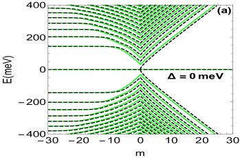
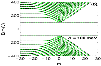
Figure 2: Energy levels as a function of the angular momentum $m$ for $B=15.7$ T, $r_{0}=44.3$ nm and two values of energy gap (a): $\Delta=0$ meV, (b): $\Delta=100$ meV with green curves for $\eta=1$ and black dashed curves for $\eta=-1$.

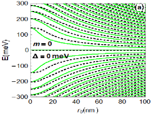
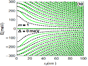
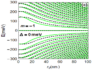
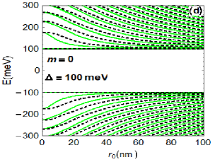
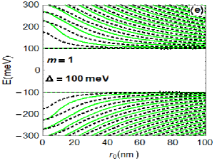
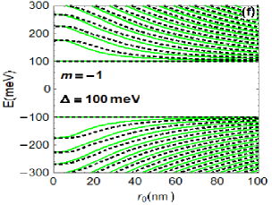
Figure 3: Energy levels as a function of the radius $r_{0}$ of quantum dot for $B=15.7$ T, three values of angular momentum and two values of energy gap. (a): $m=0$, (b): $m=1$, (c): $m=-1$ for $\Delta=0$ meV. (d): $m=0$, (e): $m=1$, (f): $m=-1$ for $\Delta=100$ meV, with green curves for $\eta=1$ and black dashed curves for $\eta=-1$.

Figure 3 presents the energy levels as a function of the radius $r_{0}$ of quantum dot for $B=15.7$ T, three values of angular momentum $m$ and two values of energy gap $\Delta$ such that (a): $m=0$, (b): $m=1$, (c): $m=-1$ for zero gap and (d): $m=0$, (e): $m=1$, (f): $m=-1$ for a gap $\Delta=100$ meV. As before, the solid and dashed lines correspond, respectively to the two valleys $K\ (\eta=1)$ and $K^{\prime}\ (\eta=-1)$. We observe that when $r_{0}$ approaches to zero, the energy levels are degenerated and then we have the symmetry $E(m,\eta)=E(m,-\eta)$. When $r_{0}$ increases such degeneracy of the valleys $K$ and $K^{\prime}$ no longer exists, which means $E(m,\eta)\neq E(m,-\eta)$. Now when $r\to\infty$, we observe that the energy levels are almost constant. For $\Delta=0$ meV, Figures 3(a,b,c) show the presence of zero energy levels in similar way to the results derived in our previous work [20]. For the case of a gap $\Delta=100$ meV, Figures 3(d,e,f) show that the energy levels possess an energy gap $2\Delta$ between the valance and conduction bands. Additionally, we notice that the energy levels verify the antisymmetry $E(m,\eta)\neq E(-m,\pm\eta)$ and asymmetry $E(m,\eta)=-E(m,-\eta)$ relations.

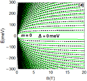
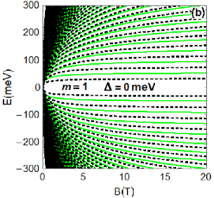
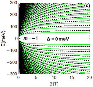
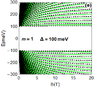
Figure 4: (color online) Energy levels as a function of the magnetic field $B$ for $r_{0}=44.3$ nm, three values of angular momentum and two values of energy gap. (a): $m=0$, (b): $m=1$, (c): $m=-1$ for $\Delta=0$ meV. (d): $m=0$, (e): $m=1$, (f): $m=-1$ for $\Delta=100$ meV, with green curves for $\eta=1$ and black dashed curves for $\eta=-1$.

In Figure 4, we present the energy levels as a function of the magnetic field $B$ for $r_{0}=44.3$ nm, three values of angular momentum $m$ and energy gap $\Delta$. More precisely, we have (a): $m=0$, $(b)$: $m=1$, (c): $m=-1$ for $\Delta=0$ meV and (d): $m=0$, (e): $m=1$, (f): $m=-1$ for $\Delta=100$ meV. It is clearly seen that for a weak magnetic field ($B\to 0$), there are many degenerate energy states corresponding to all angular momentum, for the valleys $K$ and $K^{\prime}$, in the form of a continuous energy band $E(B,\eta)=E(B,-\eta)$[21, 20]. On the other hand, it is interesting to note that there are creation of gaps when $B$ increases as shown in Figures 4(a,b,c) even in the absence of energy gap ($\Delta=0$ meV). Now we observe in Figures 4(d,e,f) that the values $\Delta=100$ meV increases the energy gap between valence and conduction bands. Then the energy gap can be used as a tunable parameter to control and adjust the energy levels.

Now let us see what happen for high magnetic field case. Indeed, by increasing $B$ we show that the degenerate levels for each $m$ are lifted due to the broken symmetry, i.e. $E(B,\eta)\neq E(B,-\eta)$. Consequently, we can find an explicit expression for the energy levels involving Landau levels $n$ in addition to angular momentum $m$

$$E_{nm}=\pm E_{0}\sqrt{n+\delta^{2}+\frac{|m_{\text{eff}}|+m_{\text{eff}}+1+\eta}{2}},\qquad n=0,1,2,\cdots$$ (30)

which can be derived by using (15) and requiring the condition $a=-n$. In this case, the confluent hypergeometric function will be replaced by the Laguerre one [22]. In Figure 5 we present the energy levels $E_{nm}$ for $\Delta=0$ meV in panels (a,b) and $\Delta=100$ meV in panels (c,d) with Landau levels $n=0,\cdots,4$. We observe that $E_{nm}$ show an asymmetric behavior between the valence and conduction bands, i.e. $E(m,\eta)=-E(m,\eta)$ [20]. In the absence of energy gap ($\Delta=0$ meV), we notice that the energy level $n=0$ is not a degenerate state for the valleys $K$ and $K^{\prime}$ because for $m<4$ it is no-null for $\eta=1$ but null for $\eta=-1$. While the other Landau levels are degenerate states for these two valleys as shown in panels (a,b). In the presence of energy gap ($\Delta\neq 0$), it is clear from panels (c,d) that all the energy levels are degenerated for the two valleys and there is an increase in the energy gap between the valence and conduction bands.

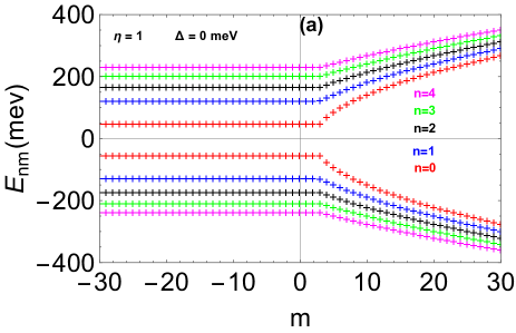
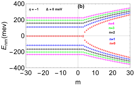
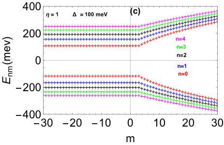
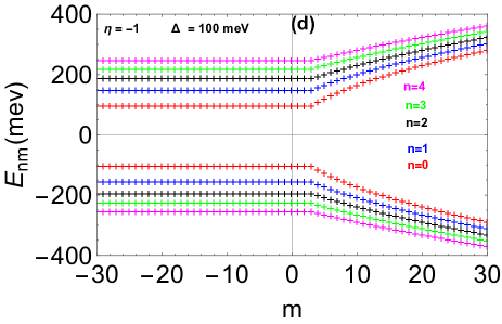
Figure 5: (color online) Energy levels $E_{nm}$ as a function of the angular momentum $m$ for $B=12$ T and five Landau levels $n=0,\cdots 4$. (a): $\Delta=0$ meV, (c): $\Delta=100$ meV for $\eta=1$ and (b): $\Delta=0$ meV, (d): $\Delta=100$ meV for $\eta=-1$.

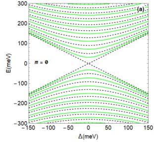
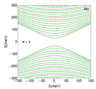
Figure 6: (color online) Energy levels as a function of the energy gap $\Delta$ for $B=15.7$ T, $r_{0}=44.3$ nm and three values of angular momentum $m$. (a): $m=0$, (b): $m=1$, (c): $m=-1$, with green curves for $\eta=1$ and black dashed curves for $\eta=-1$.

The dependence of the energy levels on the energy gap $\Delta$ is shown in Figure 6 for a magnetic field $B=15.7$ T, radius $r_{0}=44.3$ nm and three values of angular momentum $m$ with (a): $m=0$, (b): $m=1$ and (c): $m=-1$. Note that the solid and dashed lines correspond to the two valleys $K\ (\eta=1)$ and $K^{\prime}\ (\eta=-1)$, respectively. We observe that the energy levels show a parabolic behavior with a minimum corresponds to $\Delta=0$ meV and satisfy two symmetry relations such that $E(\Delta,\eta)=-E(\Delta,\eta)$ and $E(\Delta,\eta,m=1)=E(\Delta,\eta,m=-1)$. For $m=0$ in Figure 6(a), it is clearly seen the existence of the state $\eta=-1$ (black dashed curves) inside the gap. On the other hand, for $m=\pm 1$ in Figures 6(b,c), we notice that the energy levels have a energy gap even for $\Delta=0$. This result is quantitatively similar to that found for a quantum ring consisting of a single layer of graphene [23].

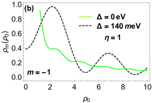
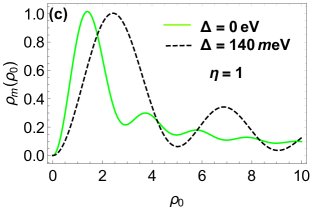
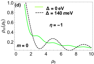
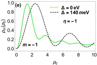
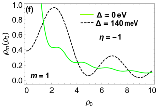
Figure 7: (color online) Radial probability $\rho_{m}(\rho_{0})$ as a function of the normalized radius $\rho_{0}=\frac{r_{0}}{l_{B}}$ of quantum dot for $B=15$ T, $E=160$ meV, $m=0,-1,1$. (a,b,c): $\eta=1$, (d,e,f): $\eta=-1$. $\Delta=0$ meV: green curves and $\Delta=140$ meV: black dashed curves.

Figure 7 presents the radial probability $\rho_{m}(\rho_{0})$ as a function of the normalized radius $\rho_{0}=\frac{r_{0}}{l_{B}}$ of quantum dot for $B=15$ T, $E=160$ meV and $m=0,-1,1$ with $\Delta=0$ meV (green) and $\Delta=140$ meV (black dashed). We notice the symmetries $\rho_{m}(\rho_{0},\eta)=\rho_{m}(\rho_{0},-\eta)$ for $m=0$ as shown in panels (a,d) and $\rho_{m}(\rho_{0},\eta)=\rho_{-m}(\rho_{0},-\eta)$ for $m\neq 0$ as presented in panels (b,f) and (c,e). We observe that when $\rho_{0}$ decreases $\rho_{m}(\rho_{0})$ tends to a maximum value near $\rho_{0}=2$. On the other hand, we have zero radial probability in the vicinity of $\rho_{0}=0$ for $m=1$ where $\eta=1$ see panel (c) and for $m=-1$ where $\eta=-1$ see panel (e). In addition, the radial probability approximately oscillates with damping as $\rho_{0}$ increases [20]. We notice that the presence of energy gap ($\Delta\neq 0$) causes a shift of $\rho_{m}(\rho_{0})$ when one moves away from the center of quantum dot and also causes a decrease in the damping of oscillations observed in the case where $\Delta=0$.

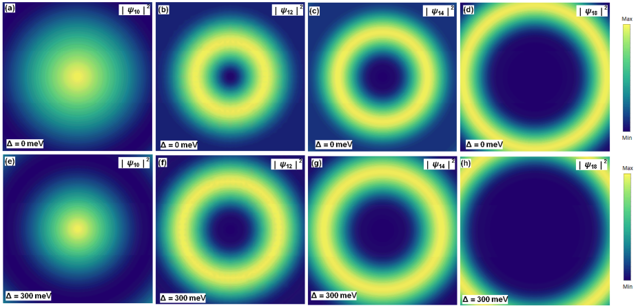
Figure 8: (color online) Spatial density $|\psi_{nm}|^{2}$ in the vicinity of the quantum dot for $\eta=\pm 1$, $B=15.7$ T. (a): ($n=1$, $m=0$), (b): ($n=1$, $m=2$), (c): ($n=1$, $m=4$), (d): ($n=1$, $m=8$) for $\Delta=0$ meV and (e): ($n=1$, $m=0$), (f): ($n=1$, $m=2$), (g): ($n=1$, $m=4$), (h): ($n=1$, $m=8$) for $\Delta=300$ meV.

Figure 8 shows the electron density of charge carriers in the quantum dot for $B=15.7$ T and some particular values of the quantum numbers $n$ and $m$. We observe that the electron density has maxima at the center of quantum dot for $m=0$ [24]. Such maxima decrease when the energy gap ($\Delta\neq 0$) is considered as it can be seen clearly by comparing panels (a,b,c,d) for $\Delta=0$ meV and panels (e,f,g,h) for $\Delta=300$ meV. On the other hand, for the case $m\neq 0$, the electron density shows a minima at the center of quantum dot [24], which increase for $\Delta\neq 0$ as can be seen by looking at panels (b,c,d) for $\Delta=0$ meV and panels (f,g,h) for $\Delta=300$ meV.

4 Conclusion

We have studied the electronic properties of a system consisting of a quantum dot surrounded by a graphene sheet with energy gap $\Delta$ in the presence of a magnetic field. By solving the Dirac equation with two bands, in the vicinity of the two valleys $K$ and $K^{\prime}$, we have derived the eigenspinors. Thanks to the boundary condition, we have obtained an analytical formula including all physical parameters characterizing our system to describe the energy levels.

We have shown that the energy levels present an asymmetry between the valence and the conduction bands, i.e. $E(B,\Delta,m,\eta)=-E(B,\Delta,m,\eta)$. For a very small size of QD ($r_{0}\to 0$) the energy levels correspond to $K$ ($\eta=1$) and $K^{\prime}$ $\eta=-1$) valleys are degenerate, that is to say $E(m,\eta)=E(m,-\eta)$. It was observed that when the size becomes large the degenerate of the valleys $K$ and $K^{\prime}$ is broken $E(m,\eta)\neq E(m,-\eta)$. We have shown that for a weak magnetic field $B\to 0$, there are many states of degenerate energy corresponding to all the angular moments $m$ for the valleys $K$ and $K^{\prime}$ in the form of a band of continuous energy. By increasing the magnetic field, the degenerate levels for each $m$ are raised because the symmetry is broken. In each representation of the energy levels shows that the introduction of energy gap $\Delta\neq 0$ leads to an increase in the gap between the valence and conduction bands.

As far as the radial probability $\rho_{m}(\rho_{0})$ is concerned, we have obtained two symmetries such that $\rho_{m}(\rho_{0},\eta)=\rho_{m}(\rho_{0},-\eta)$ for zero angular momentum $m=0$ and $\rho_{m}(\rho_{0},\eta)=\rho_{-m}(\rho_{0},-\eta)$ for a non-zero angular momentum $m\neq 0$. We have shown that the radial probability presents a maximum when the normalized radius $\rho_{0}$ of quantum dot tends towards the value 2. It was noticed that the introduction of energy gap ($\Delta\neq 0$) decreases the effect of the damping provided on the oscillation of $\rho_{m}(\rho_{0})$ in comparison with the case where $\Delta=0$. Furthermore, we have shown that the electron density presents maxima at the center of quantum dot for $m=0$ whereas for $m\neq 0$ it has minima.

References

- [1] K. S. Novoslov, A. K. Geim, S. V. Morozov, D. jiang, Y. Zhang, S. V. Dubonos, I. V. Grigorieva, and A. A. Firsov, Science 306, 666 (2004).
- [2] A. H. Castro Neto, F. Guinea, N. M. R. Peres, K. S. Novoselov, and A. K. Geim, Rev. Mod. Phys. 81, 109 (2009).
- [3] Y. Zhang, Y. W. Tan, H. L. Störnmer, and P. Kim, Nature 438, 201 (2005).
- [4] G. Jo, M. Choe, C. Y. Cho, J. H. Kim, W. Park, S. Lee, W. K. Hong, T. W. Kim, S. J. Park, B. H. Honng, Y. H. Kahng, and T. Lee, Nanotechnology 21, 175201 (2010).
- [5] C. Berger, Z. Song, X. Li, X. Wu, N. Brown, C. Naud, D. Mayou, T. Li, J. Hass, A. N. Marchenkov, E. H. Conrad, P. N. First, and W. A. de Heer, Science 312, 1191 (2006).
- [6] T. Ohta, A. Bostwick, T. Seyller, K. Horn, and E. Rotenberg, Science 313, 951 (2006).
- [7] A. V. Rozhkov, G. Giavaras, Y. P. Bliokh, V. Freilikher, and F. Nori, Phys. Rep. 503, 77 (2011).
- [8] B. Trauzettel, D. V. Bulaev, D. Loss, and G. Burkard, Nat. Phys. 3, 192 (2007).
- [9] J. H. Bardarson, M. Titov, and P. W. Brouwer, Phys. Rev. Lett. 102, 226803 (2009).
- [10] Z. Zhang, K. Chang, and F. M. Peeters, Phys. Rev. B 77, 235411 (2008).
- [11] M. Zarenia, A. Chaves, G. A. Farias, and F. M. Peeters, Phys. Rev. B 84, 245403 (2011).
- [12] M. Ezawa, Phys. Rev. B 76, 245415 (2007).
- [13] A. Matulis and F. M. Peeters, Phys. Rev. B 77, 115423 (2008).
- [14] P. Hewageegana and V. Apalkov, Phys. Rev. B 77, 245426 (2008).
- [15] T. Ohta, A. Bostwick, T. Seyller, K. Horn and E. Roten, Science 313, 951 (2006).
- [16] H. Min, B. Sahu, S. K. Banerjee, and A. H. MacDonald, Phys. Rev. B 75, 155115 (2007).
- [17] S. Schnez, K. Ensslin, M. Sigrist, and T. Ihn, Phys. Rev. B 78, 195427 (2008).
- [18] I. Snyman, Phys. Rev. B 80, 054303 (2009).
- [19] N. Myoung, J. Ryu, H. Chul Park, S. Joo Lee, and S. Woo, Phys. Rev. B 100, 045427 (2019).
- [20] A. Belouad, B. Lemaalem, A. Jellal, and H. Bahlouli, Mater. Res. Express 7, 015090 (2020).
- [21] M. Mirzakhani, M. Zarenia, A. Ketabi D. R. da Costa, and F. M. Peeters, Phys. Rev B 93, 165410 (2016).
- [22] P. Recher, J. Nilsson, G. Burkard, and B. Trauzettel, Phys. Rev. B 79, 085407 (2009).
- [23] M. Zarenia, J. Milton Pereira, A. Chaves, F. M. Peeters, and G. A. Farias, Phy. Rev B 81, 045431 (2010).
- [24] C. Schulz. R. L. Heinisch, and H. Fehske, Quantum Matter, 4, 346 (2015).